Towards Quantum Machine Learning with Tensor Networks
Abstract
Machine learning is a promising application of quantum computing, but challenges remain as near-term devices will have a limited number of physical qubits and high error rates. Motivated by the usefulness of tensor networks for machine learning in the classical context, we propose quantum computing approaches to both discriminative and generative learning, with circuits based on tree and matrix product state tensor networks that could have benefits for near-term devices. The result is a unified framework where classical and quantum computing can benefit from the same theoretical and algorithmic developments, and the same model can be trained classically then transferred to the quantum setting for additional optimization. Tensor network circuits can also provide qubit-efficient schemes where, depending on the architecture, the number of physical qubits required scales only logarithmically with, or independently of the input or output data sizes. We demonstrate our proposals with numerical experiments, training a discriminative model to perform handwriting recognition using a optimization procedure that could be carried out on quantum hardware, and testing the noise resilience of the trained model.
I Introduction
For decades, quantum computing has promised to revolutionize certain computational tasks. It now appears that we stand on the eve of the first experimental demonstration of a quantum advantage Boixo et al. (2016). With noisy, intermediate scale quantum computers around the corner, it is natural to investigate the most promising applications of quantum computers and to determine how best to harness the limited, yet powerful resources they offer.
Machine learning is a very appealing application for quantum computers because the theories of learning and of quantum mechanics both involve statistics at a fundamental level, and machine learning techniques are inherently resilient to noise, which may allow realization by near-term quantum computers operating without error correction. But major obstacles include the limited number of qubits in near-term devices and the challenges of working with real data. Real data sets may contain millions of samples, and individual samples are typically vectors with hundreds or thousands of components. Therefore one would like to find quantum algorithms that can perform meaningful tasks for large sets of high-dimensional samples even with a small number of noisy qubits.
The quantum algorithms we propose in this work implement machine learning tasks—both discriminative and generative—using circuits equivalent to tensor networks Östlund and Rommer (1995); Orus (2014); Verstraete et al. (2008), specifically tree tensor networks Fannes et al. (1992); Lepetit et al. (2000); Tagliacozzo et al. (2009); Hackbusch and Kühn (2009) and matrix product states Östlund and Rommer (1995); Vidal (2003); Schollwöck (2011). Tensor networks have recently been proposed as a promising architecture for machine learning with classical computers Cohen et al. (2016); Novikov et al. ; Stoudenmire and Schwab (2016), and provide good results for both discriminative Novikov et al. ; Stoudenmire and Schwab (2016); Levine et al. (2017); Liu et al. (2017); Khrulkov et al. (2017); Stoudenmire (2018); Glasser et al. (2018) and generative learning tasks Han et al. (2017); Guo et al. (2018).
The circuits we will study contain many parameters which are not determined at the outset, in contrast to quantum algorithms such as Grover search or Shor factorization Grover (1996); Shor (1997). Only the circuit geometry is fixed, while the parameters determining the unitary operations must be optimized for the specific machine learning task. Our approach is therefore conceptually related to the quantum variational eigensolver Peruzzo et al. (2014); McClean et al. (2016) and to the quantum approximate optimization algorithms Farhi et al. (2014), where quantum circuit parameters are discovered with the help of an auxiliary classical algorithm.

The application of such hybrid quantum-classical algorithms to machine learning was recently investigated by several groups for labeling Farhi and Neven (2018); Schuld and Killoran (2018) or generating data Gao et al. (2017); Benedetti et al. (2018); Mitarai et al. (2018). The proposals of Refs. Farhi and Neven, 2018; Benedetti et al., 2018; Mitarai et al., 2018; Schuld and Killoran, 2018 are related to approaches we propose below, but consider very general classes of quantum circuits. This motivates the question: is there a subset of quantum circuits which are especially natural or advantageous for machine learning tasks? Tensor network circuits might provide a compelling answer, for three main reasons:
-
1.
Tensor network models could be implemented on small, near-term quantum devices for input and output dimensions far exceeding the number of physical qubits. If the hardware permits the measurement of one of the qubits separately from the others, then the number of physical qubits needed can be made to scale either logarithmically with the size of the processed data, or independently of the data size depending on the particular tensor network architecture. Models based on tensor networks may also have an inherent resilience to noise. We explore both of these aspects in Section IV.
-
2.
There is a gradual crossover from classically simulable tensor network circuits to circuits that require a quantum computer to evaluate. With classical resources, tensor network models already give very good results for supervised Novikov et al. ; Stoudenmire and Schwab (2016); Liu et al. (2017); Stoudenmire (2018) and unsupervised Han et al. (2017); Stoudenmire (2018) learning tasks. The same models—with the same dataset size and data dimension—can be used to initialize more expressive models requiring quantum hardware, making the optimization of the quantum-based model faster and more likely to succeed. Algorithmic improvements in the classical setting can be readily transferred to the quantum setting as well.
-
3.
There is a rich theoretical understanding of the properties of tensor networks Orus (2014); Verstraete et al. (2008); Schollwöck (2011); Evenbly and Vidal (2011); Hastings (2007); Östlund and Rommer (1995), and their relative mathematical simplicity (involving only linear operations) will likely facilitate further conceptual developments in the machine learning context, such as interpretability and generalization. Properties of tensor networks, such as locality of correlations, may provide a favorable inductive bias for processing natural data Levine et al. (2017). One can prove rigorous bounds on the noise-resilience of quantum circuits based on tensor networks Kim and Swingle (2017).
All of the experimental operations necessary to implement tensor network circuits are available for near-term quantum hardware. The capabilities required are preparation of product states; one- and two-qubit unitary operations; and measurement in the computational basis.
In what follows, we first describe our proposed frameworks for discriminative and generative learning tasks in Section II. Then we present results of a numerical experiment which demonstrates the feasibility of the approach using operations that could be carried out with an actual quantum device in Section III. We conclude by discussing how the learning approaches could be implemented with a small number of physical qubits and by addressing their resilience to noise in Section IV.
II Learning with Tensor Network Quantum Circuits
The family of tensor networks we will consider—tree tensor networks and matrix product states—can always be realized precisely by a quantum circuit; see Fig. 1. Typically, the quantum circuits corresponding to tensor networks are carefully devised to make them efficient to prepare and manipulate with classical computers Vidal (2008). With increasing bond dimension, tree and matrix product state tensor gradually capture a wider range of states, which translates into more expressive and powerful models within the context of machine learning.
For very large bond dimensions, tree and matrix product tensor networks can eventually encompass the entire state space. But when the bond dimensions become too high, the cost of the classical approach becomes prohibitive. By implementing tensor network circuits on quantum hardware instead, one could go far beyond the space of classically tractable models.
In this section, we first describe our tensor-network based proposal for performing discriminative tasks with quantum hardware. The goal of a discriminative model is to produce a specific output given a certain class of input; for example, assigning labels to images. Then we describe our proposal for generative tasks, where the goal is to generate samples from a probability distribution inferred from a data set. For more background on various types of machine learning tasks, see the recent review Ref. Mehta et al., 2018.
For clarity of presentation, we shall make use of multi-qubit unitary operations in this work. However we recognize that in practice such unitaries must be implemented using a more limited set of few-qubit operations, such as the universal gate sets of one- and two-qubit operators. Whether it is more productive to classically optimize over more general unitaries then “compile” these into few-qubit operations as a separate step, or to parameterize the models in terms of fewer operations from the outset remains an interesting and important practical question for further work.
II.1 Discriminative Algorithm
To explain the discriminative tensor network framework that we propose here, assume that the input to the algorithm takes the form of a vector of real numbers , with each component normalized such that . For example, such an input could correspond to a grayscale image with pixels, with individual entries encoding normalized grayscale values. We map this vector to a product state on N qubits according to the feature map proposed in Ref. Stoudenmire and Schwab, 2016:
| (1) |
Such a state can be prepared by starting from the computational basis state , then applying a single qubit unitary to each qubit .
The model we then propose can be seen as an iterative coarse-graining procedure that parameterizes a CPTP (completely positive trace preserving) map from an N-qubit input space to a small number of output qubits encoding the different possible class labels. The circuit takes the form of a tree, with qubit lines connecting each subtree to the rest of the circuit. We call such qubit lines “virtual qubits” to connect with the terminology of tensor networks, where tensor indices internal to the network are called virtual indices. A larger can capture a larger set of functions, just as a tensor network with a sufficiently large bond dimension can parameterize any N-index tensor.
At each step, we take of the qubits resulting from one of the unitary operations of the previous step, or subtree, and from another subtree and act on them with another parameterized unitary transformation (possibly together with some ancilla qubits—not shown). Then of the qubits are discarded, while the other proceed to the next node of the tree, that is, the next step of the circuit. In our classical simulations we trace over all discarded qubits, while on a quantum computer, we would be free to ignore or reset such qubits.
Once all unitary operations defining the circuit have been carried out, one or more qubits serve as the output qubits. (Which qubits are outputs is designated ahead of time.) The most probable state of the output qubits determines the prediction of the model, that is, the label the model assigns to the input. To determine the most probable state of the output qubits, one performs repeated evaluations of the circuit for the same input in order to estimate their probability distribution in the computational basis.
We show the quantum circuit of our proposed procedure in Fig. 2. In the case of image classification, it is natural to always group input qubits based on pixels coming from nearby regions of the image, with a tree structure illustrated schematically in Fig. 3.
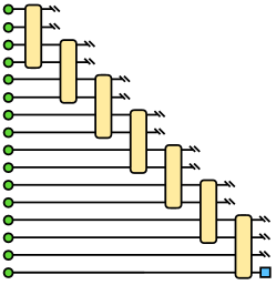
A closely related family of models can be devised based on matrix product states. An example is illustrated in Fig. 4 showing the case of . Matrix product states (MPS) can be viewed as maximally unbalanced trees, and differ from the binary tree models described above in that after each unitary operation on inputs only one set of qubits are passed to the next node of the network. Such models are likely a better fit for data that has a one-dimensional pattern of correlations, such as time-series, language, or audio data.
II.2 Generative Algorithm
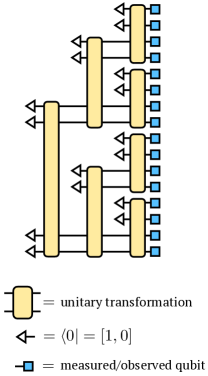
The generative algorithm we propose is nearly the reverse of the discriminative algorithm, in terms of its circuit architecture. The algorithm produces random samples by first preparing a quantum state then measuring it in the computational basis, putting it within the family of algorithms recently dubbed “Born machines” Han et al. (2017); Gao et al. (2017); Benedetti et al. (2018). But rather than preparing a completely general state, we shall consider specific patterns of state preparation corresponding to tree and matrix product state tensor networks. This provides the advantages discussed in the introduction, such as connections to classical tensor network models and the ability to reduce the number of physical qubits required, which will be discussed further in Section IV.
The generative algorithm based on a tree tensor network (shown in Fig. 5) begins by preparing qubits in a reference computational basis state , then entangling these qubits by unitary operations. Another set of qubits are prepared in the state . Half of these are grouped with the first entangled qubits, and half with the second entangled qubits. Two more unitary operations are applied to each new grouping of qubits; the outputs are now split into four groups; and the process repeats for each group. The process ends when the total number of qubits processed reaches the size of the output one wants to generate.
Once all unitaries acting on a certain qubit have been applied, this qubit can be measured. The measured output of all of the qubits in the computational basis represents one sample from the generative model.
III Numerical Experiments
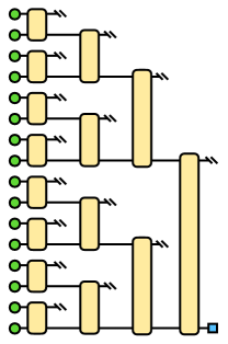
To show the feasibility of implementing our proposal on a near-term quantum device, we trained a discriminative model based on a tree tensor network for a supervised learning task, namely labeling image data. The specific network architecture we used is shown as a quantum circuit in Fig. 7. When viewed as a tensor network, this model has a bond dimension of . This stems from the fact that after each unitary operation entangles two qubits, only one of the qubits is acted on at the next scale (next step of the circuit).
III.1 Loss Function
Our eventual goal is to select the parameters of our circuit such that we can confidently assign the correct label to a new piece of data by running our circuit a small number of times. To this end, we choose the loss function which we want to minimize starting with the following definitions. Let be the model parameters; be an element of the training data set; and let be the probability of the model to output a label for a given input . Because we consider the setting of supervised learning, the correct labels are known for the training set inputs, and define to be the correct label for the input . Now define
| (2) |
as the probability of the incorrect output state which has the highest probability of being observed. Then, define the loss function for a single input to be
| (3) |
and the total loss function to be
| (4) |
The “hyper-parameters” and are to be chosen to give good empirical performance on a validation data set. Essentially, we assign a penalty for each element of the training set where the gap between probability of assigning the true label and the probability of assigning the most likely incorrect label is less than . This loss function allows us to concentrate our efforts during training on making sure that we are likely to assign the correct label after taking the majority vote of several executions of the model, rather than trying to force the model to always output the correct label in each separate run.
III.2 Optimization
Of course, we are interested in training our circuit to generalize well to unobserved inputs, so instead of optimizing over the entire distribution of data as in Eq. 4, we optimize the loss function over a subset of the training data and compare to a held-out set of test data. Furthermore, because the size of the training set for a typical machine learning problem is so large (60,000 examples in the case of the MNIST data set), it would be impractical to calculate the loss over all of the training data at each optimization step. Instead, we follow a standard approach in machine learning and randomly select a mini-batch of training examples at each iteration. Then, we use the following stochastic estimate of our true training loss (recalling that represents the current model parameters):
| (5) |
In order to faithfully test how our approach would perform on a near-term quantum computer, we have chosen to minimize our loss function using a variant of the simultaneous perturbation stochastic approximation (SPSA) algorithm which was recently used to find quantum circuits approximating ground states in Ref. Kim and Swingle, 2017 and was originally developed in Ref. Spall, 1998.
Essentially, each step of SPSA estimates the gradient of the loss function by performing a finite difference calculation along a random direction and updates the parameters accordingly. In our experimentation, we have also found it helpful to include a momentum term , which mixes a fraction of previous update steps into the current update. We outline the algorithm we used in more detail below.
-
1.
Initialize the model parameters randomly, and set to zero.
-
2.
Choose appropriate values for the constants, that define the optimization procedure.
-
3.
For each , set and , and randomly partition the training data into mini-batches of images. Perform the following steps using each mini-batch:
-
(a)
Generate random perturbation in parameter space.
-
(b)
Evaluate , with defined as in Eq. 5.
-
(c)
Set
-
(d)
Set
-
(a)
III.3 Results
We trained circuits with a single output qubit at each node to recognize grayscale images of size belonging to one of two classes using the SPSA optimization procedure described above. The images were obtained from the MNIST data set of handwritten digits Yann LeCun , and we show results below for classifiers trained to distinguish between each of the 45 pairs of handwritten digits 0 through 9.
The unitary operations applied at each node in the tree were parameterized by writing them as where is a Hermitian matrix (the matrices were allowed to be different for each node). The free parameters were chosen to be the elements forming the diagonal and upper triangle of each Hermitian matrix, resulting in exactly 1008 free parameters for the image recognition task. The mini-batch size and the other hyper-parameters for the training procedure and the loss function were hand-tuned by running a small number of experiments, using the SigOpt sig software package, with the goal of obtaining the most rapid and consistent performance (averaged over the different digit pairs) on a validation data set.
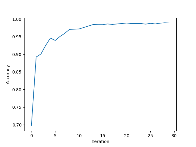
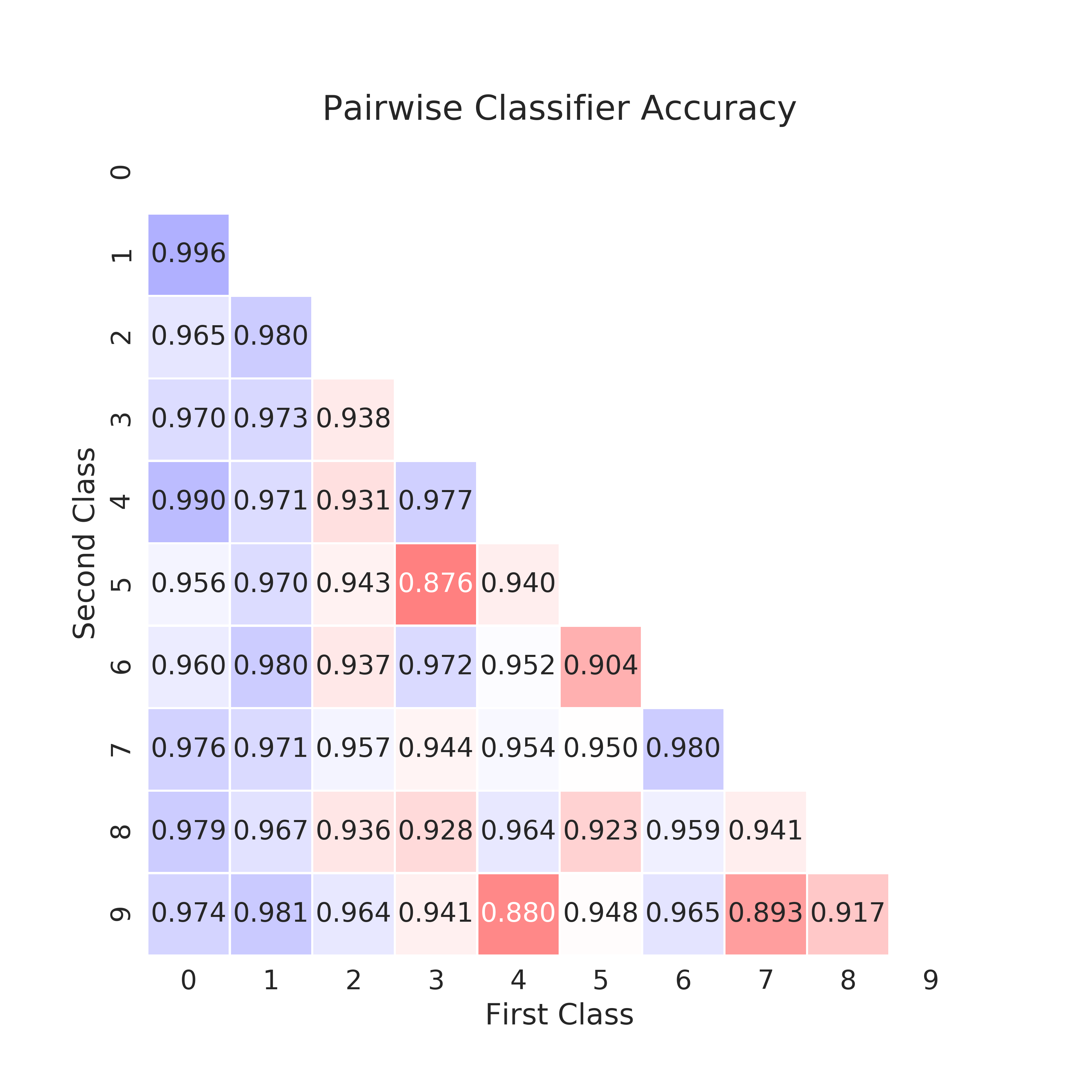
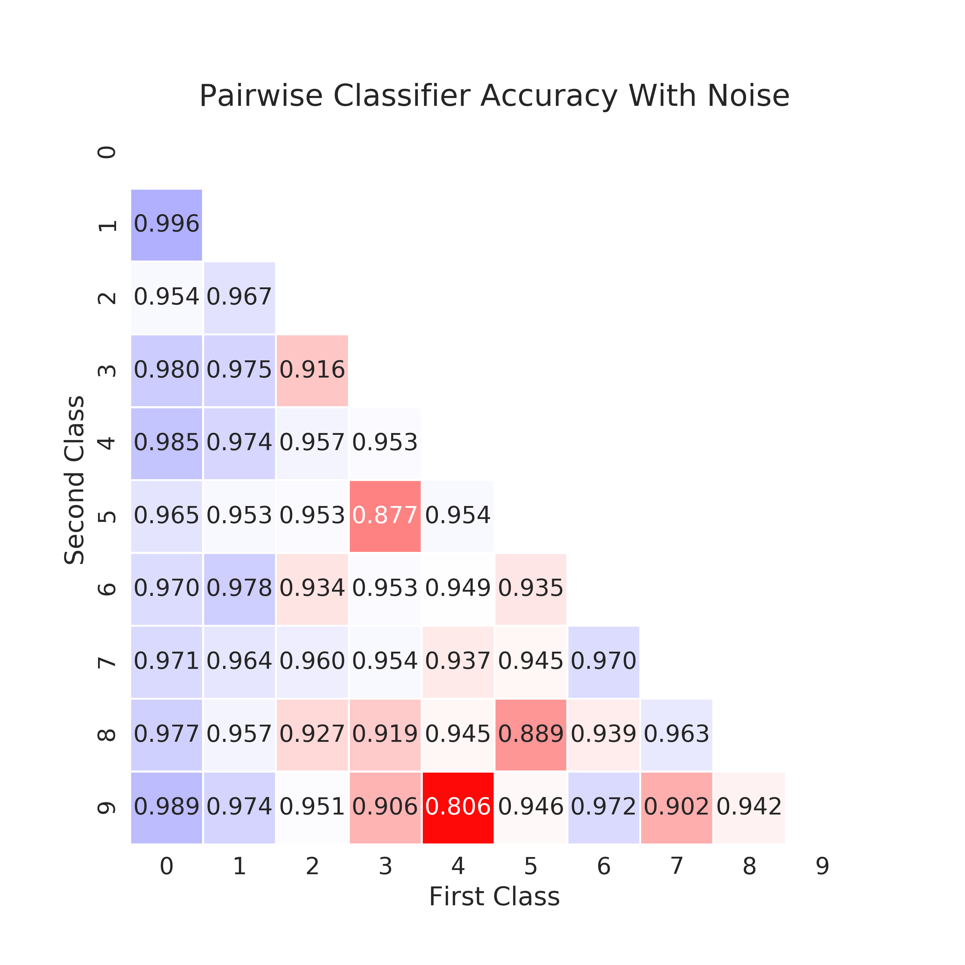
Ultimately, we found that networks trained with the choices were able to achieve an average test accuracy above 95%. The accuracies of the individual pairwise classifiers are tabulated in Fig. 9, and data from a representative example of the training process for one of the easier pairs to classify is shown in 8. We observed significant differences in performance across the different pairs, partly owing, perhaps, to the difficulty of distinguishing similar digits using 64 pixel images. We also note that different choices of hyper-parameters could significantly affect which pairs were classified most accurately.
IV Implementation on Near-Term Devices
A key advantage of carrying out machine learning tasks with models equivalent to tree or matrix product tensor networks is that they could be implemented using a very small number of physical qubits. The key requirement is that the hardware must allow the measurement of individual physical qubits without further disturbing the state of the other qubits, a capability also required for certain approaches to quantum error correction Córcoles et al. (2015). Below we will first discuss how the number of qubits needed to implement either a discriminative or generative tree tensor network model can be made to scale only logarithmically in both the data dimension and in the bond dimension of the network. Then we will discuss the special case of matrix product state tensor networks, which can be implemented with a number of physical qubits that is independent of the input or output data dimension.
Another key advantage of using tensor network models on near-term devices could be their robustness to noise, which will certainly be present in any near-term hardware. To explore the noise resilience of our models, we present a numerical experiment where we evaluate the model trained in Section III with random errors, and observe whether it can still produce useful results.
IV.1 Qubit-Efficient Tree Network Models
To discuss the minimum qubit resources needed to implement general tree tensor network models, recall the notion of the virtual qubit number from Section II. This is the number of qubit lines connecting each subtree to higher nodes in the tree. Viewed as a tensor network, the bond dimension , or dimension of the internal tensor indices, is given by .
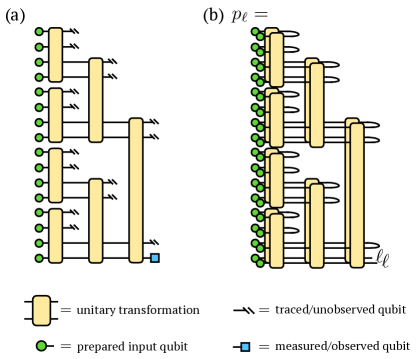
For example, the tree shown in Fig. 7 has and a bond dimension of . The tree shown in Fig. 10 has and . When discussing these models in general terms, it suffices to consider only unitary operations acting on qubits, since at each node of the tree, two subtrees (two sets of qubits) are entangled together.
Given only the ability to perform state preparation and unitary operations, it would take physical qubits to evaluate a discriminative tree network model on inputs. However, if we also allow the step of measurement and resetting of certain qubits, then the number of physical qubits required to process inputs given virtual states passing between each node can be significantly reduced to just .
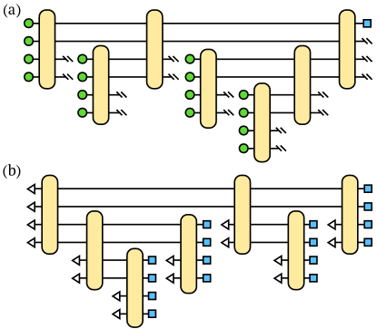
To see why, consider the circuit showing the most qubit-efficient scheme for implementing the discriminative case Fig. 10(a). For a given , the number of inputs that can be processed by a single unitary is . Then of the qubits can be measured and reused, but the other qubits must remain entangled. So only new qubits must be introduced to process more inputs. From this line of reasoning and the observation that , one can deduce the result .
For generative tree network models, generating outputs with virtual qubits requires the same number of physical qubits as for the discriminative case; this can be seen by observing that the pattern of unitaries is just the reverse of the discriminative case for the same and . Fig. 10 shows the most qubit-efficient way to sample a generative tree models for the case of virtual and output qubits, requiring only physical qubits.
Though a linear growth of the number of physical qubits as a function of virtual qubit number may seem more prohibitive compared to the logarithmic scaling with , even a small increase in would lead to a significantly more expressive model. From the point of view of tensor networks the expressivity of the model is usually measured by the bond dimension . In terms of the bond dimension, the number of qubits needed thus scales only as . The largest bond dimensions used in state-of-the-art classical tensor network calculations are around or about . So for or more virtual qubits one would quickly exceed the power of any classical tensor network calculation we are aware of.
IV.2 Qubit-Efficient Matrix Product Models
A matrix product state (MPS) tensor network is a special case of a tree tensor network that is maximally unbalanced. This gives an MPS certain advantages without sacrificing expressivity for one-dimensional distributions, as measured by the maximum entanglement entropy it can carry across bipartitions of the input or output space, meaning a division of from .
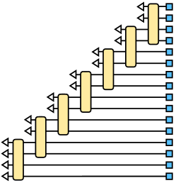
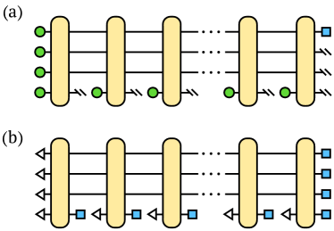
Given the ability to measure and reset a subset of physical qubits, a key advantage of implementing a discriminative or generative tensor network model based on an MPS is that for a model with virtual qubits, an arbitrary number of inputs or outputs can be processed by using only physical qubits. The circuits illustrating how this can be done are shown in Fig. 11.
The implementation of the discriminative algorithm shown in Fig. 11(a) begins by preparing and entangling input qubit states. One of the qubits is measured and reset to the next input state. Then all qubits are entangled and a single qubit measured and re-prepared. Continuing in this way, one can process all of the inputs. Once all inputs are processed, the model output is obtained by sampling one or more of the physical qubits.
To implement the generative MPS algorithm shown in Fig. 11(b), one prepares all qubits to a reference state and after entangling the qubits, one measures and records a single qubit to generate the first output value. This qubit is reset to the state and all the qubits are then acted on by another qubit unitary. A single qubit is again measured to generate the second output value, and the algorithm continues until outputs have been generated.
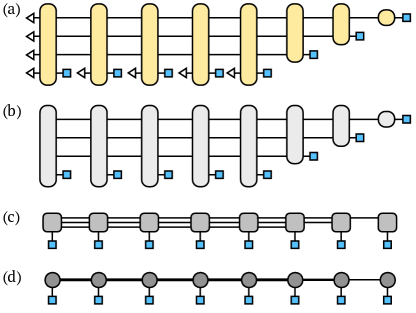
To understand the equivalence of the generative circuit of Fig. 11(b) to conventional tensor diagram notation for an MPS, interpret the circuit diagram Fig. 12(a) as a tensor network diagram, treating elements such as reference states as tensors or vectors . One can contract or sum over the reference state indices and merge any qubit indices into a single index of dimension . The result is a standard MPS tensor network diagram Fig. 12(d) for the amplitude of observing a particular set of values of the measured qubits.
IV.3 Noise Resilience
Any implementation of our proposed approach on near-term quantum hardware will have to contend with a significant level of noise due to qubit and gate imperfections. But one intuition about noise effects in our tree models is that an error which corrupts a qubit only scrambles the information coming from the patch of inputs belonging to the past “causal cone” of that qubit. And because the vast majority of the operations occur near the leaves of the tree, the most likely errors therefore correspond to scrambling only small patches of the input data. We note that a good classifier should naturally be robust to small deformations and corruptions of the input, and, in fact, adding various kinds of noise during training is a commonly used strategy in classical machine learning. Based on these intuitions, we expect our circuits could demonstrate a high level of tolerance to noise.
In order to quantitatively understand the robustness of our proposed approach to noise on quantum hardware, we study how performance is affected by independent amplitude-damping and dephasing channels applied to each qubit. In particular, we investigate how this error model would affect the pairwise tree network discriminative models of the type described in Section II.1 and shown in Fig. 7.
The specific error model we implemented is the following: during the contraction step of node in the model evaluation, we compose amplitude damping and dephasing noise channels acting on its left and right children and , mapping and . Any completely positive trace-preserving noise channel can be expressed in the operator-sum representation as , where . Here the Kraus operators for the amplitude damping channel are (in the -basis)
while for the dephasing channel the Kraus operators are
To evaluate model performance under realistic values of and on current hardware, we determine and based on the continuous-time Kraus operators of these channels, which depend on the duration of the two-qubit gate , the coherence time of the qubits, and the dephasing time of the qubits. Specifically, and . Realistic values for the time scales are and , , corresponding to and . But numerical experiments with these values showed almost no observable noise effects, so we consider an even more conservative parameter set with and reduced by an order of magnitude, such that and .
We plot the resulting test accuracies in Fig. 13, noting that the Kraus operator formalism allows us to directly calculate the reduced density matrix of the labeling qubit under the effects of our noise model, therefore no explicit sampling of noise realizations is needed. Given that the coherence times used for the plot are easily achievable even on today’s very early hardware platforms, the results shown in Fig. 13 are encouraging: many of the models give a test accuracy only slightly reduced from the noiseless case Fig. 9. The largest reduction was for the digit ‘4’ versus digit ‘9’ model, which dropped from a test accuracy of 0.88 to 0.806. Interestingly this was also the model with the worst performance in the noiseless case. The typical change in test accuracy across all of the models due to the noise was about 0.004.
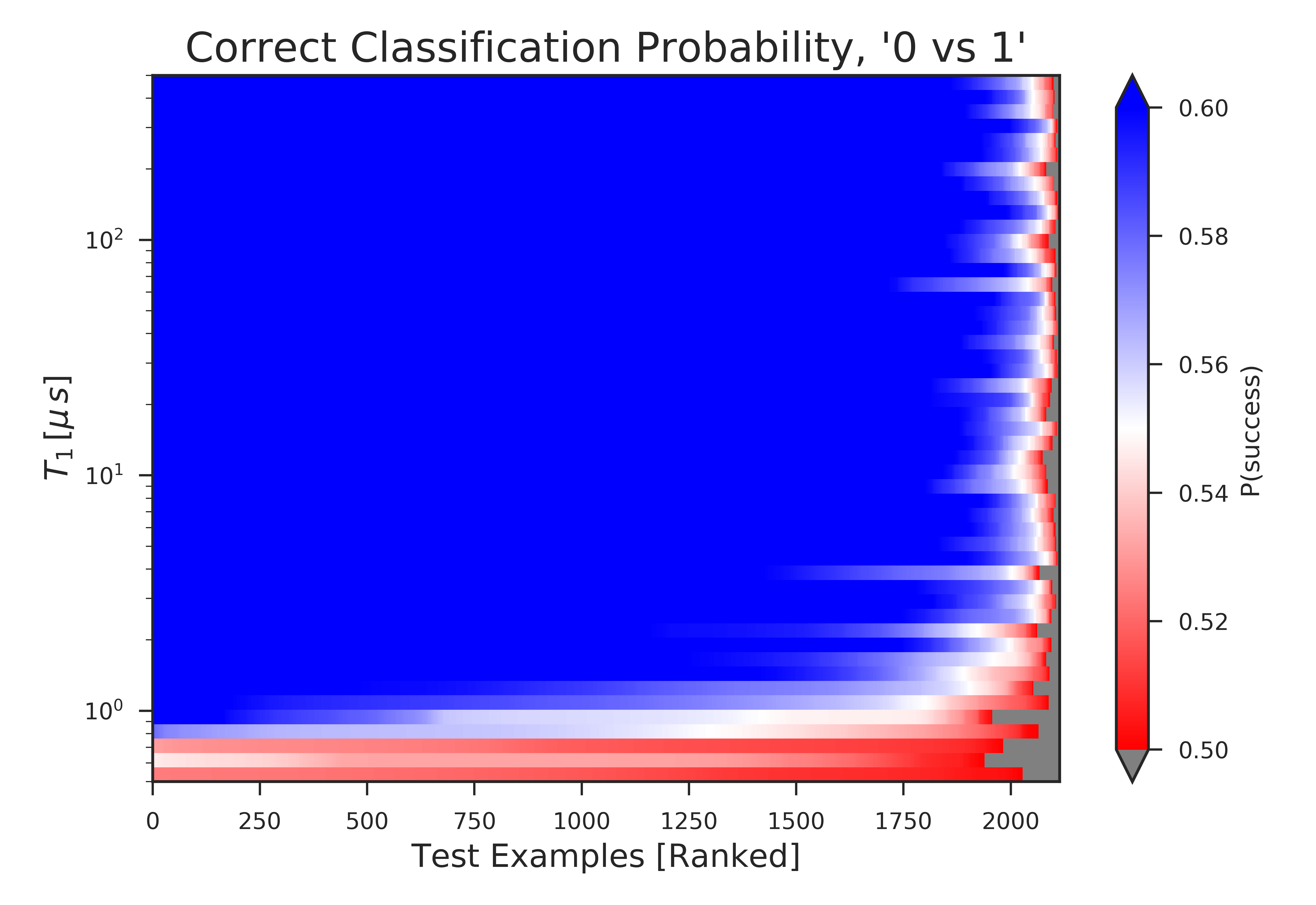
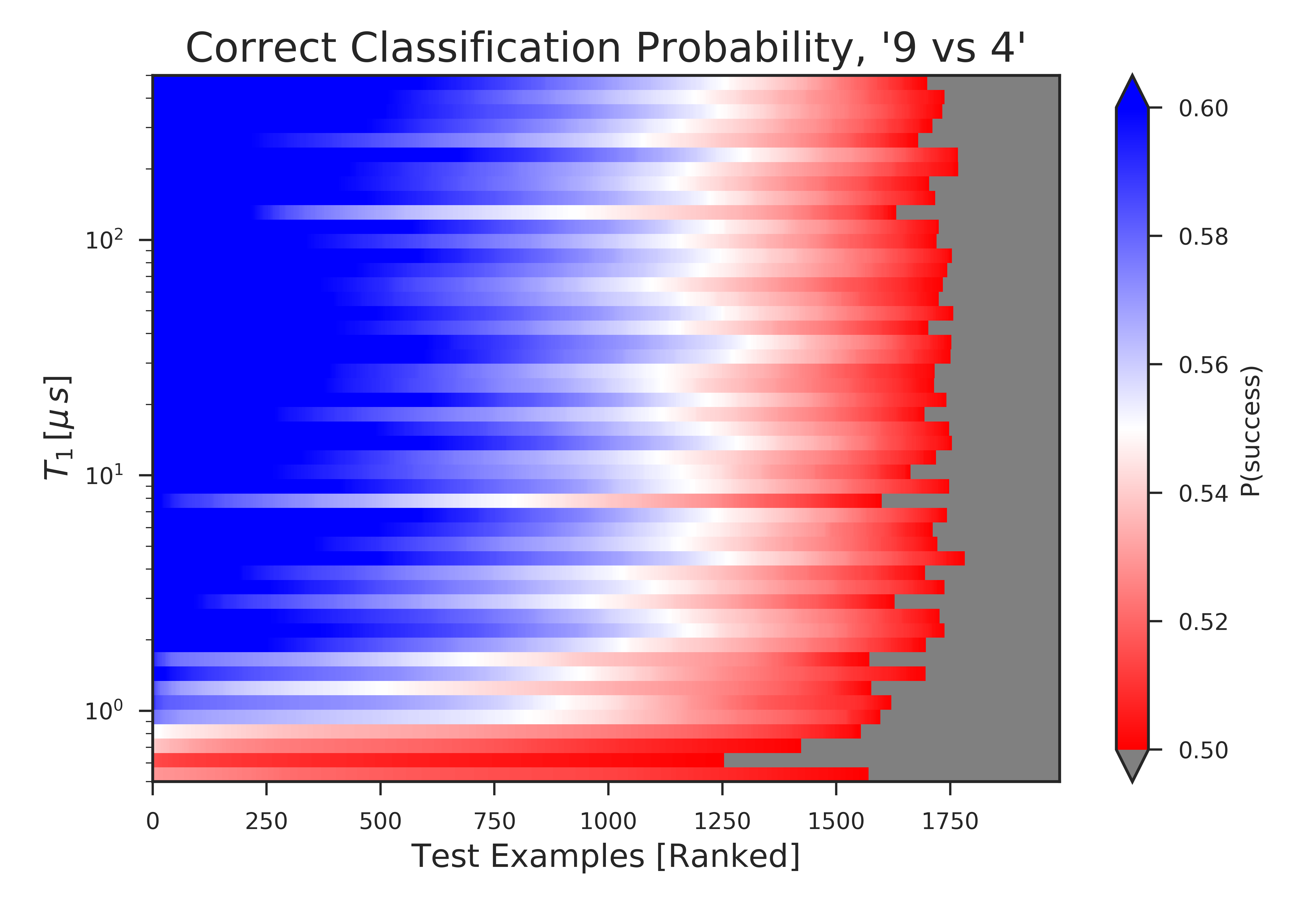
To mitigate the effect of noise when classifying a particular image, one can evaluate the quantum circuit some small number of times and choose the label which is most frequently observed. For example, one could take a majority vote from 500 executions and classify and correctly classify an image whose individual probability of success is with almost accuracy. In order to shed a more detailed light on our approach’s robustness to noise, we plot in Fig. 14 the individual success probabilities for classifying each test example (-axis), sorted by their probabilities for ease of visualization, over a range of decoherence times (-axis). The two panels show two different models, one trained to distinguish images of digits ‘0’ versus ‘1’ ; the other digits ‘9’ versus ‘4’. These models were trained and evaluated at various levels of noise using the same training hyper-parameters that were found to give a good performance at . The ratio between the dephasing time and the coherence time was held at a fixed ratio .
We see that, for the examples which our models correctly classify in the low noise limit, the success probability remains appreciably greater than for a wide range of noise levels. In both diagrams the y-axis is scaled so that coherence times achievable by today’s hardware occur two thirds of the way up from the bottom. Interestingly, we note that the success probabilities saturate at coherence times much shorter than this, and only drop off dramatically at values near . The high performance of our model over a broad swath of tested coherence and dephasing times suggests that the effects of noise on our approach can be dramatically mitigated by the combination of the hybrid quantum/classical training procedure and a small number of repetitions with a majority voting scheme. We find these results encouraging as empirical evidence that the limited-width “causal cone” structure possessed by models of this type may have inherent noise robustness properties.
V Discussion
Many of the features that make tensor networks appealing for classical algorithms also make them a promising framework for quantum computing. Tensor networks provide a natural hierarchy of increasingly complex quantum states, allowing one to choose the appropriate amount of resources for a given task. They also enable specialized algorithms which can make efficient use of valuable resources, such as reducing the number of qubits needed to process high dimensional data. An optimized, classically tractable tensor network can be used to initialize the parameters of a more powerful model implemented on quantum hardware. Doing so would alleviate issues associated with random initial parameters, which can place circuits in regions of parameter space with vanishing gradients McClean et al. (2018).
While the approach to optimization we considered in our numerical experiments worked well, algorithms which are more specialized to the tensor network architecture could be devised. For example, by defining an objective for each subtree of a tree network it could be possible to train subtrees separately Stoudenmire (2018). Likewise, the MPS architecture has certain orthogonality or light-cone properties which mean that only the tensors to the left of a certain physical index determine its distribution; this property could also be exploited for better optimization.
Another very interesting future direction would be to gain a better understanding of the noise resilience of tensor network machine learning algorithms. We performed some simple numerical experiments to show that these algorithms can tolerate a high level of noise, but additional empirical demonstrations as well as a theoretical explanation of how generic this property is would be very useful. In an interesting recent work, Kim and Swingle investigated tensor networks within a quantum computing framework for finding ground states of local Hamiltonians Kim and Swingle (2017). One of their results was a rigorous bound on the sensitivity of the algorithm output to noise, which relied on specific properties of tensor networks. It would be very interesting adapt their bound to the machine learning context.
Other tensor network architectures besides trees and MPS also deserve further investigation in the context of quantum algorithms. The PEPS family of tensor networks are specially designed to capture two-dimensional patterns of correlations Schwarz et al. (2012, 2013). The MERA family of tensor networks, retain certain benefits of tree tensor networks but have more expressive power, and admit a natural description as a quantum circuit Vidal (2008); Kim and Swingle (2017).
Tensor networks strike a careful balance between
expressive power and computational efficiency, and can be viewed as a particularly useful
and natural class of quantum circuits. Based on the rich theoretical
understanding of their properties and powerful algorithms for optimizing them,
we are optimistic they will provide many interesting avenues for quantum machine learning
research.
Acknowledgements
We thank Dave Bacon, Norm Tubman, Alejandro Perdomo-Ortiz, Mark Nowakowski, Vinay Ramasesh, Dar Dahlen, and Lei Wang for helpful discussions. The work of W. Huggins and K. B. Whaley was supported by the U.S. Department of Energy, Office of Science, Office of Advanced Scientific Computing Research, Quantum Algorithm Teams Program, under contract number DE-AC02-05CH11231. Computational resources were provided by NIH grant S10OD023532, administered by the Molecular Graphics and Computation Facility at UC Berkeley.
References
- Boixo et al. (2016) Sergio Boixo, Sergei V. Isakov, Vadim N. Smelyanskiy, Ryan Babbush, Nan Ding, Zhang Jiang, John M. Martinis, and Hartmut Neven, “Characterizing quantum supremacy in near-term devices,” arxiv:1608.00263 (2016).
- Östlund and Rommer (1995) Stellan Östlund and Stefan Rommer, “Thermodynamic limit of density matrix renormalization,” Phys. Rev. Lett. 75, 3537–3540 (1995).
- Orus (2014) Roman Orus, “A practical introduction to tensor networks: Matrix product states and projected entangled pair states,” Annals of Physics 349, 117 – 158 (2014).
- Verstraete et al. (2008) F. Verstraete, V. Murg, and J. I. Cirac, “Matrix product states, projected entangled pair states, and variational renormalization group methods for quantum spin systems,” Advances in Physics 57, 143–224 (2008).
- Fannes et al. (1992) M. Fannes, B. Nachtergaele, and R. F. Werner, “Finitely correlated states on quantum spin chains,” Communications in Mathematical Physics 144, 443–490 (1992).
- Lepetit et al. (2000) M.-B. Lepetit, M. Cousy, and G.M. Pastor, “Density-matrix renormalization study of the hubbard model [4]on a bethe lattice,” The European Physical Journal B - Condensed Matter and Complex Systems 13, 421–427 (2000).
- Tagliacozzo et al. (2009) L. Tagliacozzo, G. Evenbly, and G. Vidal, “Simulation of two-dimensional quantum systems using a tree tensor network that exploits the entropic area law,” Phys. Rev. B 80, 235127 (2009).
- Hackbusch and Kühn (2009) W. Hackbusch and S. Kühn, “A new scheme for the tensor representation,” Journal of Fourier Analysis and Applications 15, 706–722 (2009).
- Vidal (2003) Guifré Vidal, “Efficient classical simulation of slightly entangled quantum computations,” Phys. Rev. Lett. 91, 147902 (2003).
- Schollwöck (2011) U. Schollwöck, “The density-matrix renormalization group in the age of matrix product states,” Annals of Physics 326, 96–192 (2011).
- Cohen et al. (2016) Nadav Cohen, Or Sharir, and Amnon Shashua, “On the expressive power of deep learning: A tensor analysis,” 29th Annual Conference of Learning Theory , 698–728 (2016).
- (12) Alexander Novikov, Mikhail Trofimov, and Ivan Oseledets, “Exponential machines,” arxiv:1605.03795 (2016) .
- Stoudenmire and Schwab (2016) E.M. Stoudenmire and David J Schwab, “Supervised learning with tensor networks,” in Advances In Neural Information Processing Systems 29 (2016) pp. 4799–4807, arxiv:1605.05775 .
- Levine et al. (2017) Yoav Levine, David Yakira, Nadav Cohen, and Amnon Shashua, “Deep learning and quantum entanglement: Fundamental connections with implications to network design,” (2017), arxiv:1704.01552 .
- Liu et al. (2017) Ding Liu, Shi-Ju Ran, Peter Wittek, Cheng Peng, Raul Blázquez García, Gang Su, and Maciej Lewenstein, “Machine learning by two-dimensional hierarchical tensor networks: A quantum information theoretic perspective on deep architectures,” arxiv:1710.04833 (2017).
- Khrulkov et al. (2017) Valentin Khrulkov, Alexander Novikov, and Ivan Oseledets, “Expressive power of recurrent neural networks,” arxiv:1711.00811 (2017).
- Stoudenmire (2018) E.M. Stoudenmire, “Learning relevant features of data with multi-scale tensor networks,” arxiv:1801.00315 (2018).
- Glasser et al. (2018) Ivan Glasser, Nicola Pancotti, and J. Ignacio Cirac, “Supervised learning with generalized tensor networks,” arxiv:1806.05964 (2018).
- Han et al. (2017) Zhao-Yu Han, Jun Wang, Heng Fan, Lei Wang, and Pan Zhang, “Unsupervised generative modeling using matrix product states,” arxiv:1709.01662 (2017).
- Guo et al. (2018) Chu Guo, Zhanming Jie, Wei Lu, and Dario Poletti, “Matrix product operators for sequence to sequence learning,” arxiv:1803.10908 (2018).
- Grover (1996) Lov K. Grover, “A fast quantum mechanical algorithm for database search,” in Proceedings of the Twenty-eighth Annual ACM Symposium on Theory of Computing, STOC ’96 (ACM, New York, NY, USA, 1996) pp. 212–219.
- Shor (1997) Peter W. Shor, “Polynomial-time algorithms for prime factorization and discrete logarithms on a quantum computer,” SIAM Journal on Computing 26, 1484–1509 (1997).
- Peruzzo et al. (2014) Alberto Peruzzo, Jarrod McClean, Peter Shadbolt, Man-Hong Yung, Xiao-Qi Zhou, Peter J. Love, Alán Aspuru-Guzik, and Jeremy L. O’Brien, “A variational eigenvalue solver on a photonic quantum processor,” Nature Communications 5, 4213 (2014).
- McClean et al. (2016) Jarrod R McClean, Jonathan Romero, Ryan Babbush, and Alan Aspuru-Guzik, “The theory of variational hybrid quantum-classical algorithms,” New Journal of Physics 18, 023023 (2016).
- Farhi et al. (2014) Edward Farhi, Jeffrey Goldstone, and Sam Gutmann, “A quantum approximate optimization algorithm,” arxiv:1411.4028 (2014).
- Farhi and Neven (2018) Edward Farhi and Hartmut Neven, “Classification with quantum neural networks on near term processors,” arxiv:1802.06002 (2018).
- Schuld and Killoran (2018) Maria Schuld and Nathan Killoran, “Quantum machine learning in feature hilbert spaces,” arxiv:1803.07128 (2018).
- Gao et al. (2017) Xun Gao, Zhengyu Zhang, and Luming Duan, “An efficient quantum algorithm for generative machine learning,” arxiv:1711.02038 (2017).
- Benedetti et al. (2018) Marcello Benedetti, Delfina Garcia-Pintos, Yunseong Nam, and Alejandro Perdomo-Ortiz, “A generative modeling approach for benchmarking and training shallow quantum circuits,” arxiv:1801.07686 (2018).
- Mitarai et al. (2018) Kosuke Mitarai, Makoto Negoro, Masahiro Kitagawa, and Keisuke Fuji, “Quantum circuit learning,” arxiv:1803.00745 (2018).
- Evenbly and Vidal (2011) G. Evenbly and G. Vidal, “Tensor network states and geometry,” Journal of Statistical Physics 145, 891–918 (2011).
- Hastings (2007) M.B. Hastings, “An area law for one-dimensional quantum systems,” J. Stat. Mech. 2007, P08024 (2007).
- Kim and Swingle (2017) Isaac H. Kim and Brian Swingle, “Robust entanglement renormalization on a noisy quantum computer,” arxiv:1711.07500 (2017).
- Vidal (2008) G. Vidal, “Class of quantum many-body states that can be efficiently simulated,” Phys. Rev. Lett. 101, 110501 (2008).
- Mehta et al. (2018) Pankaj Mehta, Marin Bukov, Ching-Hao Wang, Alexandre G.R. Day, Clint Richardson, Charles K. Fisher, and David J. Schwab, “A high-bias, low-variance introduction to machine learning for physicists,” arxiv:1803.08823 (2018).
- Spall (1998) James C Spall, “An overview of the simultaneous perturbation method for efficient optimization,” Johns Hopkins apl technical digest 19, 482–492 (1998).
- (37) Christopher J.C. Burges Yann LeCun, Corinna Cortes, “MNIST handwritten digit database,” http://yann.lecun.com/exdb/mnist/ .
- (38) .
- Córcoles et al. (2015) A. D. Córcoles, Easwar Magesan, Srikanth J. Srinivasan, Andrew W. Cross, M. Steffen, Jay M. Gambetta, and Jerry M. Chow, “Demonstration of a quantum error detection code using a square lattice of four superconducting qubits,” Nature Communications 6, 6979 EP – (2015).
- McClean et al. (2018) Jarrod R. McClean, Sergio Boixo, Vadim N. Smelyanskiy, Ryan Babbush, and Hartmut Neven, “Barren plateaus in quantum neural network training landscapes,” arxiv:1803.11173 (2018).
- Schwarz et al. (2012) Martin Schwarz, Kristan Temme, and Frank Verstraete, “Preparing projected entangled pair states on a quantum computer,” Phys. Rev. Lett. 108, 110502 (2012).
- Schwarz et al. (2013) Martin Schwarz, Kristan Temme, Frank Verstraete, David Perez-Garcia, and Toby S. Cubitt, “Preparing topological projected entangled pair states on a quantum computer,” Phys. Rev. A 88, 032321 (2013).