Tensions between direct measurements of the lens power spectrum from Planck data
Abstract
We apply a recently developed method to directly measure the gravitational lensing power spectrum from CMB power spectra to the Planck satellite data. This method allows us to analyze the tension between the temperature power spectrum and lens reconstruction in a model independent way. Even when allowing for arbitrary variations in the lensing power spectrum, the tension remains at the 2.4 level. By separating the lensing and unlensed high redshift information in the CMB power spectra, we also show that under CDM the two are in tension at a similar level whereas the unlensed information is consistent with lensing reconstruction. These anomalies are driven by the smoother acoustic peaks relative to CDM at . Both tensions relax slightly when polarization data are considered. This technique also isolates the one combination of the lensing power spectrum multipoles that the Planck CMB power spectra currently constrain and can be straightforwardly generalized to future data when CMB power spectra constrain multiple aspects of lensing which are themselves correlated with lensing reconstruction.
I Introduction
Measurements of anisotropies in the cosmic microwave background (CMB) have helped to establish CDM as the standard cosmological model and measure its parameters with high precision. Currently, CMB data are precise enough to detect the effects of gravitational lensing (see Lewis and Challinor (2006) for a review) at high significance Smith et al. (2007); Hirata et al. (2008); Hanson et al. (2013); Das et al. (2011); Keisler et al. (2011); Ade et al. (2014); Keisler et al. (2015); Ade et al. (2016a, b); Sherwin et al. (2016). This secondary signal depends on growth of structure in the universe, which can be leveraged to measure better certain parameters in CDM like the sum of the neutrino masses and search for new physics beyond the standard cosmological model.
Information carried by the lensing potential can be recovered either by measuring its effect on CMB power spectra, in particular the smoothing of the acoustic peaks Seljak (1996), or by higher point combinations of the temperature and polarization maps. The latter is possible, because gravitational lensing generates a correlation between measured CMB fields and their gradients Zaldarriaga (2000). This correlation can be used to reconstruct , for example using quadratic combinations of maps Hu (2001); Hu and Okamoto (2002); Okamoto and Hu (2003) or iterative approaches Hirata and Seljak (2003); Smith et al. (2012). The reconstructed potential then serves as a new observable whose power spectrum contains cosmological information.
Within the context of CDM, measurements of the Planck satellite show internal tension – at significance over 2 – in the amount of lensing apparently present in the temperature power spectra data Ade et al. (2016c); Aghanim et al. (2017); Addison et al. (2016); Ade et al. (2014). At the same time, the amount of lensing detected through the lensing reconstruction seems to be consistent with the CDM model. Such tensions are interesting, as they could indicate residual systematics in the data, which would have to be understood before performing delensing using the reconstructed Carron et al. (2017). They might even represent hints of new physics beyond the CDM model.
In this paper, we perform a model-independent investigation of information in the Planck temperature and polarization power spectra and assess its tension with lensing reconstruction. As opposed to previous studies of the tension, which considered changes to only the amplitude of the gravitational lensing potential relative to the CDM model, we allow for more general changes. This enables us to probe the possibility that models beyond CDM might resolve this lensing tension.
Specifically, we implement the method introduced in Motloch et al. (2017); Motloch and Hu (2017), in which the lensing potential is constrained directly. This method isolates the precise aspect of that temperature and polarization power spectra constrain, which enables a more incisive and model-independent assessment of any tension with reconstruction. Additionally, this work represents the first test of the method on real data. This method will become increasingly useful in the future as CMB temperature and polarization power spectra constrain more than just the amplitude of the gravitational lensing potential and enable consistency tests that are largely immune to cosmic variance.
This paper is organized as follows. In §II we summarize the Planck likelihoods used in this work and introduce our technique for probing the gravitational lensing potential. In §III we use this method to derive Planck lensing constraints from CMB power spectra and lens reconstruction. In §IV we then evaluate the significance of the tensions between the two and with CDM. We discuss our findings in §V.
II Lensing methodology
In this section we first introduce the data and analysis method used in this work. After that we detail the technique we use to directly measure the gravitational lensing potential from the data; this technique is employed to probe Planck lensing tensions in the later sections.
| Label | Power spectra | -range | Binned? | Name |
|---|---|---|---|---|
TT |
TT | yes | plik_dx11dr2_HM_v18_TT |
|
TTTEEE |
TT,TE,EE | yes | plik_dx11dr2_HM_v18_TTTEEE |
|
lowT |
TT | no | commander_rc2_v1.1_l2_29_B |
|
lowTEB |
TT,TE,EE,BB | no | lowl_SMW_70_dx11d_2014_10_03_v5c_Ap |
|
PP |
yes | smica_g30_ftl_full_pp |
||
liteTT |
TT | yes | plik_lite_v18_TT |
II.1 Data sets and MCMC
For the analyses in this work we use the publicly released Planck 2015
likelihoods*1*1*1https://www.cosmos.esa.int/web/planck/pla for the power spectra of the CMB temperature, polarization and
of the gravitational lensing potential reconstructed from their maps as summarized in
Table 1. Joint use of multiple likelihoods will be denoted by a plus sign
connecting them.
For the analyses using only the lensing reconstruction likelihood PP, correction for the biases is performed
using the best fit power spectra to TT+lowTEB likelihoods assuming the six parameter
CDM model. The likelihood liteTT, which we use for the lens principal component
construction and checking robustness of the results below, is a high- temperature likelihood, with
the foreground parameters pre-marginalized over. Otherwise, we marginalize over the standard foreground parameters with their default priors, where
applicable.
For the analyses in this paper we use the Markov Chain Monte Carlo (MCMC) code CosmoMC*2*2*2https://github.com/cmbant/CosmoMC Lewis and Bridle (2002) to sample the posterior probability in the various parameter spaces described in the next section. Each of our chains has a sufficient number of samples such that the Gelman-Rubin statistic Gelman and Rubin (1992) falls below 0.01.
II.2 Lens PC measurement technique
We can measure gravitational lensing of the CMB from both temperature and polarization power spectra and from lensing reconstruction. While lensing reconstruction maps directly measure the lens power spectrum , in the standard analysis of the temperature and polarization power lensing is inferred from the set of model parameters. This makes it difficult to compare these two distinct sources of lensing information directly since information from the latter is embedded in the cosmological parameter constraints. In this work we instead consider model-independent constraints on . For this purpose we introduce a basis of effective parameters which determine arbitrary variations around a fixed fiducial power spectrum as
| (1) |
In this setup, constraining from the data corresponds directly to constraining the gravitational lensing potential. This should be contrasted with the common approach of introducing a phenomenological parameter which multiplies at each point in the model space and cannot be so interpreted once model parameters are marginalized over.
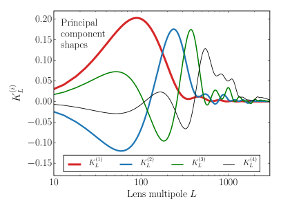
We choose such that correspond to principal components
(PCs) of
the gravitational lensing potential best measured by the Planck lensed TT power
spectrum. We determine them from the data covariance matrix provided with the
Planck likelihood liteTT using a Fisher matrix construction; the resultant eigenmodes are shown in
Fig. 1. The lowest variance mode peaks around and is
much better constrained than the second best constrained component; the Fisher matrix
forecast predicts a factor of in the ratio of variances. This is largely because
Planck data do not strongly constrain the power spectrum Smith et al. (2006)
or temperature multipoles above , which are sensitive to smaller scale
lenses.
Because are smooth functions of , we
discretize into bins of width
(see Motloch et al. (2017) for more details). Unless otherwise specified, we retain PCs in order to
fully characterize all sources of lensing information (see §III.1).
In addition to these lens parameters we take the standard CDM parameters for the unlensed CMB spectra: , the physical baryon density; , the physical cold dark matter density; , the tilt of the scalar power spectrum; , its log amplitude at Mpc-1; the optical depth through reionization, and , the angular scale of the sound horizon at recombination. We use flat priors with uninformative ranges on these parameters.
In the MCMC analyses with , these cosmological parameters are still present and determine the “unlensed” CMB fluctuations at recombination as well as the background expansion. However, they do not affect the lens potential as they would in the standard analysis. We will refer to these parameters collectively as , where the tilde is to remind the reader that the gravitational lens potential is not changed by these parameters.
The fiducial cosmological model used to calculate in Eq. (1) is taken from
the best fit flat CDM cosmological model, determined from TT+lowTEB
likelihoods assuming no primordial tensor modes and minimal
mass neutrinos ().
To reflect the latest results on the optical depth to recombination
Adam et al. (2016), we set to the value from that work and decrease
to keep constant. A lower tends to exacerbate the preference for
anomalously high lensing in the temperature power spectrum
within the CDM context but here serves only as the baseline fiducial model against
which to define .
Values of the corresponding cosmological
parameters are listed in Table *4.
| Parameter | Fiducial value |
|---|---|
| 100 | 1.041 |
In models beyond CDM, changes in the integrated Sachs-Wolfe (ISW) effect would typically affect data on the largest scales. In this work we are interested only in lensing-like effects and leave the ISW contribution at its CDM value.
Because the cosmic variance fluctuations of the lensing PCs are by at least factor eight smaller than the precision with which Planck power spectra can measure , it is not necessary to consider the lensing-induced covariance terms discussed in Benoit-Levy et al. (2012); Motloch et al. (2017) in our analysis.
III Model-independent lensing constraints
Measuring the lens principal components from the Planck temperature, polarization and lensing reconstruction power spectra provides a new means of extracting and comparing the various sources of lens information in the CMB. This comparison presents a direct and model-independent consistency test of the lensing information Motloch et al. (2017) and in the CDM model context enables an internal consistency check of the CDM parameters inferred from CMB power spectra information from recombination and from lens information. This is particularly relevant given the known preference for excess lensing in the Planck temperature data Ade et al. (2014, 2016c).
We start by characterizing the information in the lensing reconstruction data, which also determines the number of lens principal components required for our comparative analysis. We then discuss constraints on from the temperature and polarization power spectra and focus on the two leading principal components. We also derive from the recombination or unlensed information in the power spectrum in the CDM model as a check of its internal consistency. We finish by commenting on robustness of our results with respect to various analysis choices.
III.1 Reconstruction constraints
The principal component decomposition of the lens power spectrum described in §II.2 is optimized for the temperature power spectrum analysis but can also be used to analyze the reconstruction data. Even though we will be mainly interested in the first two components for comparisons with the other analyses, it is important to retain a sufficient number of higher components so that their marginalization does not affect the lower ones.
In practice we choose the number of principal components according to whether the data can constrain them better than a weak theoretical prior. We choose flat tophat priors on within a range where the variation in is within a factor of 1.5 of . These weak priors are meant to eliminate cases that would be in conflict with other measurements of large scale structure or imply unphysically large amplitude high frequency features in .
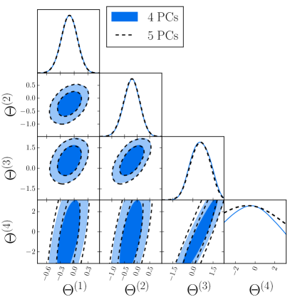
In Fig. 2 we show constraints from the lensing reconstruction
likelihood PP on the first four for the cases
where we allow four or five lens PCs to vary. For and
the edges of the box represent the prior and so the 4th component is nearly prior limited.
Correspondingly, the addition of does not significantly affect constraints
on
and which will be important for evaluation of the tensions
in the data. We therefore standardize on four lens PCs unless otherwise specified, with
higher lens PCs set to zero, which is their fiducial value.
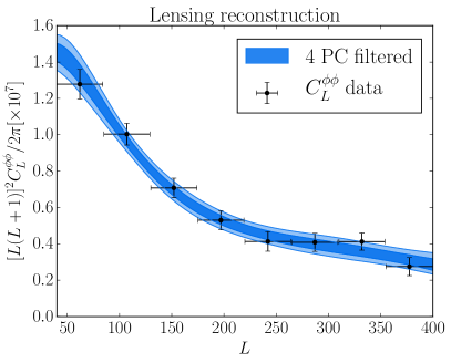
Another way to visualize why 4 PCs suffices is to construct the lens power spectrum out of them as
| (2) |
and compare it to the lens reconstruction data itself. In Fig. 3, we show this comparison. The 4 PC construction represents smooth deviations that are allowed by the data. Fluctuations that are not represented by the functional form of the PCs shown in Fig. 1 are not captured by the construction, for example the fluctuation in the data around . Thus the PC construction does not represent direct, but rather filtered, constraints on . To compare PC constraints from other sources to the lens reconstruction constraints, it is important to compare their implications for rather than directly. This PC filter has the benefit of producing smooth functional constraints utilizing the full data set at the expense of highly correlating constraints at different multipoles.
III.2 Temperature constraints
We analyze the TT+lowTEB likelihood for 4 PCs with the weak theoretical priors
discussed in the previous section.
To focus on the region consistent with lens reconstruction, we impose an
additional data-driven prior. As shown in the previous section, lensing reconstruction constrains and
significantly better than the theoretical prior from the previous section, we thus
consider restricting these two variables further. As we will see, drives
the tension between reconstruction and temperature constraints; for this reason we do not strengthen the prior on it. On the other
hand, we restrict to lie within six standard deviations from the mean value
from the reconstruction analysis that considers 4 PCs. We retain this prior even for
analyses in which is fixed to its fiducial value. We shall see that the
tension between power spectra and lensing reconstruction information on lensing
is weaker
than 6 and so this prior does not artificially increase the tension.
It therefore just excludes the parameter space that would
be grossly ruled out by reconstruction data and is used mostly for visualization
purposes.
As expected, TT+lowTEB data constrain mainly one principal
component with limited by the priors and
and completely dominated by them.
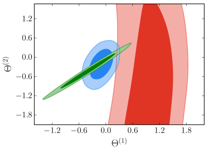
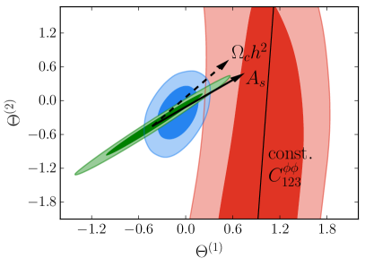
In Fig. 4 we show the constraints (red contours) in the
plane out to the edge of the prior. Because
the PCs were constructed from a Fisher forecast,
the constrained direction
is nearly but not perfectly aligned with , leaving a slight correlation between the
two parameters.
In Fig. 5 we show that the degenerate direction for the TT+lowTEB analysis
corresponds approximately to
constant
, whereas contours of constant correspond approximately to
as determined by the zero crossing of in Fig. 1.
For comparison we in Fig. 4 also show the constraints from lens reconstruction (blue contours). The two constraints are in tension with each other in that the two contours only overlap in their 95% CL regions. Moreover, this tension is model independent: no change in the shape of allowed by the 4 PCs can resolve it.
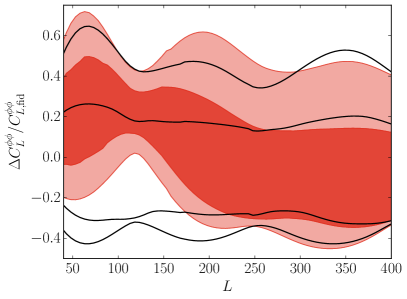
We can also visualize the TT+lowTEB constraint
on as filtered through the first 4 PCs via
Eq. (2); for
the ease of comparison we show fractional difference from the fiducial model.
In Fig. 6 we show
that posterior constraints from the TT+lowTEB data are tighter than
the prior mainly around while at high the
constraints are prior dominated.
Note that the prior is skew positive
allowing a tail to high where the probability drops slowly.
The large values of that the data prefer can therefore easily
push the CL region of the posterior beyond that of the prior,
especially around .
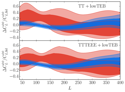
In Fig. 7 (top panel) we compare these posterior constraints on from the TT+lowTEB to those from PP.
The reconstruction data favors less power around . Although changes in the shape of can bring agreement
between the two away from this regime, tension remains there independent of the model.
We have explicitly checked that relaxing the
theoretical priors does not aggravate this tension, despite the fact that the upper bounds
from the posterior and the prior
around coincide in Fig. 6.
Within the CDM we can further study the origin of this tension.
From the same TT+lowTEB analysis, we can
predict
from information in the unlensed CMB power spectra at
each sampled parameter point under the CDM assumption. We can then translate this prediction into by
inverting
Eq. (1).
These CDM predictions, shown as the green contours in
Fig. 4, can be directly compared
with the lensing PC measurements
themselves. Some tension between the red and green
contours is visible, as they overlap only at the confidence levels; this is the lensing PC version of the
well-known lensing anomaly in the high- TT data.
Unlike , which only indirectly specifies by changing its
amplitude relative to the CDM prediction point by point in its parameter space, PCs directly change the
amplitude and shape of . This allows us to more directly quantify the
origin of lensing tension. It is straightforward to trace
back the origin of the CDM degenerate direction in the plane: arrows in Figure 5 show how these two parameters
change when we increase values of and (at fixed and other
parameters; constructed from the partial derivatives listed in
Tab. 3), which within CDM are the two parameters
with dominant effects on . Given current constraints on , the degenerate
direction is mainly aligned with that of , with a smaller contribution from . On the other hand, the lensing PC constraints from TT+lowTEB mainly
reflect and are driven by the region of the lens power spectrum that is best measured by the TT spectrum. Though
they are lens model independent, the lens reconstruction constraints are in good
agreement with the CDM constraints in green.
Furthermore, the near alignment of the directions of the CDM constraints and
the reconstruction constraints (blue) also suggest that the tension with power spectrum constraints (red)
cannot be significantly relieved by going beyond CDM.
| 82.0 | 99.1 | |
| 7.45 | 5.95 |
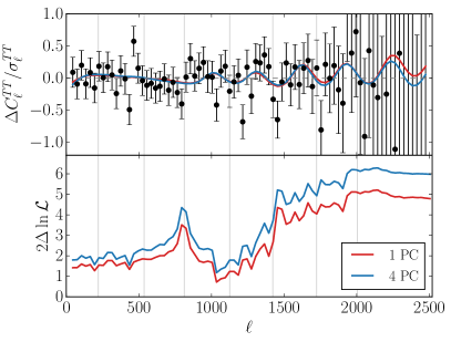
We can also compare the temperature power spectrum of the maximum likelihood CDM model with that of the maximum likelihood model with lens PCs to see what part of the temperature power spectrum data drives this preference for anomalous lensing; we show cases where either one or four lens PCs are varying from their fiducial values. In Fig. 8, we show the residuals relative to the best fit CDM model scaled by the cosmic variance errors per multipole,
| (3) |
evaluated at the fiducial CDM
model. Notice the Planck data are binned and so the standard deviations of the data can be smaller
than .
When searching for the best fit PC model, we fix the foreground
parameters to their best fit CDM values from the TT+lowTEB
likelihood, for which the visualization of the Planck data points were
derived.
In the lower panel of Fig. 8, we then show the cumulative
improvement over CDM in
of the
fit as a function of the maximum .*5*5*5Due to different binning schemes used by
the Planck collaboration for their best fit TT power spectrum and binned TT likelihood,
we use the unbinned Planck TT likelihood to obtain this plot.
The total reaches at the highest multipole employed in the analysis
when allowing four lens PCs to vary.
As is visible from the figure, of 6 comes from the first
lens PC, in agreement with our previous statement
that majority of the lensing information in the temperature power spectra is well captured
by a single lensing component.
The data points show oscillatory residuals with respect to the CDM model in the range 1250–1500 that
indicate smoother acoustic oscillations (see also
Aghanim et al. (2017); Obied et al. (2017)). Correspondingly, the largest part of the
improvement arises through fitting these residuals by increasing the smoothing due to lensing, though notable contributions come from the lowTEB part of the likelihood. The latter
is associated with the ability to lower TT power at .
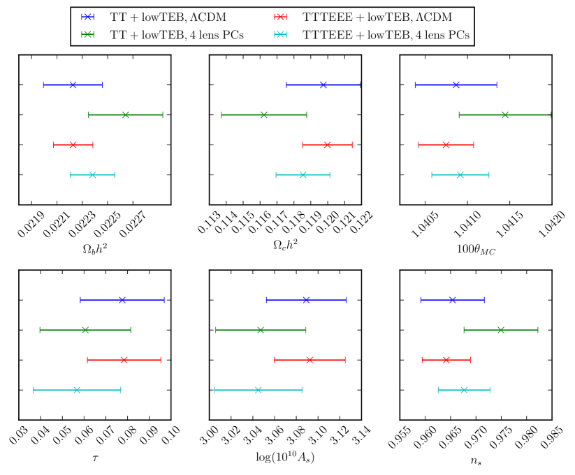
These improvements allowed by releasing from its CDM value also lead to shifts in cosmological parameters; these shifts are summarized in Figure 9, for the case where the foreground parameters are again allowed to vary. In CDM, preference for fitting the oscillatory residuals pushes values of and up, which then forces other CDM parameters to compensate. In the PC case, lensing parameters play this role and allow to drop. This drop and the associated changes in other parameters allows for a lower low- TT power with respect to the acoustic peaks and therefore also allows a better fit to the anomalously low TT power at . In models with the CDM expansion history such a drop also simultaneously raises to and can help relieve tension with the local distance ladder measurements Riess et al. (2018).
Taken at face value, these mild tensions and their alleviation with lensing PC parameters would motivate explorations of additional physics at low which modify the lens potential. However, independent of the model for the lens potential, tension with lensing reconstruction remains.
III.3 Polarization constraints
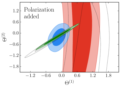
Next, we add the high- polarization constraints using the
TTTEEE+lowTEB likelihood; the various constraints on are shown
in Fig. 10. The 2015 Planck polarization data is known to be subject to
systematics that make lensing conclusions unstable Ade et al. (2016c) and thus we consider
their addition separately.
The main change is a shift in the contours to lower values of but with tighter errors. This shift is driven by the data; lensing constraints from are notably weaker and additionally favor even more lensing than does Ade et al. (2016c). With polarization, the tension between CMB power spectra and lens reconstruction constraints only mildly relaxes. This is because of the combination of the shift and the smaller errors in Fig. 10. In Fig. 7 (bottom), we also show the impact of adding polarization data on the filtered constraints. Correspondingly, polarization data only mildly decreases the significance of tension around .
The internal tension between temperature-polarization power spectra and the CDM
prediction in green relaxes somewhat more. This is because polarization favors the
high values of the best fit CDM model to
TT+lowTEB
(as shown in Fig. 9)
due to unusually strong TE constraints in the region around Obied et al. (2017). This preference is in a region
that is relatively unaffected by lensing and so remains after releasing .
Raising in CDM has the effect of increasing lensing making
the temperature-polarization power spectra and CDM somewhat more consistent.
III.4 Robustness tests
To check that the results are stable with respect to the considered number of lens
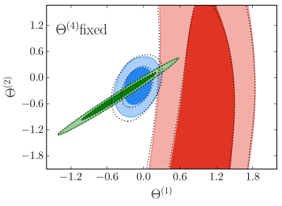
PCs, we repeat our analysis with fixed to its fiducial value. In
Fig. 11 (top) we show that this does not significantly alter the various
constraints on based on TT+lowTEB and
PP. The same conclusion holds when polarization data are added.
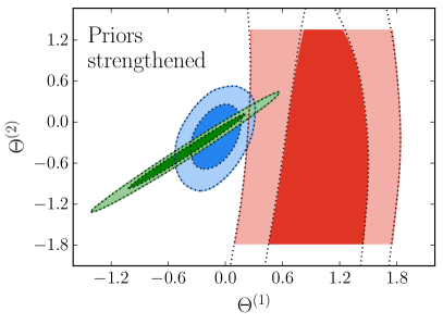
We also repeat our analysis with a tighter theoretical prior (with four lens PCs
varying) – for and we restrict the variation in
to be within a factor of 1.4 of , instead of our default
1.5, while we demand to be within five standard deviations from the
mean value determined from the PP likelihood. In
Fig. 11 (bottom) we show that impact of the theoretical prior
on the tension is negligible.
In our analysis we have so far fixed the unlensed CMB to the power spectra allowed by CDM. Given the lensing model-independence of the tension, it is also interesting to ask whether additional physics at recombination can relax it. We can never completely eliminate this possibility for resolution of tension with our methodology, as effects of this new physics might mimic lensing in the CMB power spectrum while not affecting the higher point moments important in lens reconstruction. On the other hand, we can show that the additional physics cannot be simply a change in the effective number of light relativistic species . When adding this parameter to the unlensed parameters and marginalizing over it, we find that the tension between high- TT and lensing reconstruction constraints and the internal lensing tension are both still present and similarly significant.
IV Significance of the tensions
Having illustrated the existence of lensing tensions in the Planck CMB data, we now turn to quantifying their significance. We start by defining a robust single statistic to compare between the various sources of lensing information. We then discuss the significance of the model-independent tension between lensing constraints from Planck temperature/polarization power spectra and lens reconstruction. After that we focus on a special case of CDM with a freely floating amplitude of the lensing potential, which allows us to compare with previous literature and address the significance of the internal tensions between CDM lensing constraints from within the CMB power spectra alone.
IV.1 Tension statistics
In order to quantify the tension simply and cleanly, we seek to find a single auxiliary parameter whose distribution reflects the best constraints and is as close as possible to Gaussian in each of the lensing measurements. For two such measurements, a natural tension statistic to use is the shift in the means . To the extent that the parameter posteriors are Gaussian distributed, the shift itself is predicted to be Gaussian distributed with a variance that is the sum of the two variances, . Therefore, the significance of the measured shift in units of is given by
| (4) |
| ref. data | freedom | TT+lowTEB |
TTTEEE+lowTEB |
|---|---|---|---|
PP |
4 PCs | 2.4 | 2.2 |
PP |
amplitude | 2.4 | 2.4 |
| unlensed | amplitude | 2.4 | 2.1 |
To choose the parameter itself, note that the main source of tension is the first principal component (see Fig. 4). However, to have the posterior distributions well approximated by Gaussian distributions, we instead choose
| (5) |
is independent of the higher lens PCs, as these are not constrained by the temperature and polarization power spectra and thus do not add to the tension.
The scaling factor makes the ratio of the 1 PC filtered and fiducial evaluated at (see Eq. (2)). As we will see, the main benefit of , or in general a smoothly filtered version of , is that it represents a weighted average in of the data even though it appears to be evaluated at a fixed . As such it employs the constraining power of the full range of the data. This leads to a powerful and robust tension statistic.
This should be contrasted with itself or more generally the power spectrum at any single multipole . Its value depends sensitively on the higher PCs, which increasingly fit noise fluctuations, and so represent an ineffective tension statistic when they are included. With our standard 4 PC analysis, this is not a significant problem for itself as we shall see in the next section, but by defining tension in we make it robust to higher PCs as well and immune to reoptimizing the effective multipole for each case.
IV.2 Model-independent tension
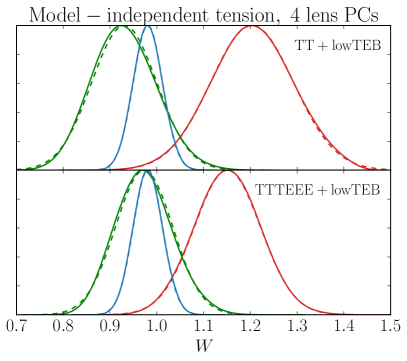
In Fig. 12, we compare posterior
distributions for determined from CMB power spectra through the TT+lowTEB, TTTEEE+lowTEB
likelihoods to that determined from reconstruction through the
PP likelihood; the two types of distributions overlap only in the tails.
Gaussians with the
same means and variances describe even these overlap regions accurately, which justifies
the use of the tension statistic .
The tension between TT+lowTEB and PP determinations of is
significant at 2.4; adding polarization data decreases the tension to 2.2.
We summarize significance of various tensions in Table 4.
We now consider several robustness checks on this tension.
Using the
foreground-marginalized high- TT likelihood liteTT instead of
TT in
the analysis leads to the same tension significance of 2.4.
When the data-driven prior on of six standard deviations from the PP
constraint is dropped, the tensions relax both by about 0.1.
This is caused by the small curvature of the posterior in the plane, visible for example in the red contour in
Fig. 10, which leads to an increased overlap with the lensing
reconstruction constraints after the projection onto .
Next we consider robustness to the constraint on the reionization optical depth .
The upcoming final release of Planck data is expected to improve and potentially change these constraints.
Furthermore, constraints on depend on the form assumed for the ionization history
that is taken
to be step-like in the standard analysis Hu and Holder (2003); Heinrich et al. (2016).
By isolating the information on the lens power spectrum itself, our tension statistic should be immune to such changes.
To quantify the
impact of possible future changes in the likelihood, we reevaluate
the tension statistic
where instead of using TT+lowTEB we
constrain using TT+lowT, together with a
prior of width 0.02, centered on either 0.04, 0.06 or 0.08.
In all three cases the tension changes by less than 0.02 from the
original result obtained using TT+lowTEB. Our conclusions are thus robust to
the low- polarization data and
likelihoods.
Contrast this with the scaled CDM approach where changes
the lens power spectrum against which is measured from the
temperature power spectrum and lens reconstruction data respectively, leading to
sensitivity of constraints to reionization assumptions.
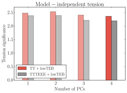
The significance of the tension between
TT+lowTEB (or TTTEEE+lowTEB) and PP determinations of does not
notably change when we decrease the freedom in varying by retaining a smaller
number of lens PCs in the analysis (see Fig. 13).
Finally, it is possible to demonstrate why is more robust than at some
that has not been specifically optimized for the model-independent lensing test.
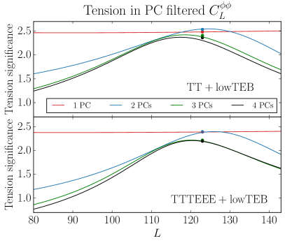
First, we can take the full 4 PC filtered construction of depicted in
Fig. 7.
We show the resulting tension as a function of in
Fig. 14 (black curves) between
PP and TT+lowTEB (or TTTEEE+lowTEB).
The tension in constraints at is similar to that in
. On the other hand, choosing other values of could
substantially degrade the ability to identify tension in these cases where the shape of is
allowed to vary.
Likewise, an alternate choice of can make the tension statistic more dependent on the number of lens PCs allowed to vary. In Fig. 14, we also show the results of analyses with 1,2 or 3 lens PCs allowed to vary, where is filtered with the same number of PCs. Again, away from the tension significance can vary widely.
IV.3 CDM and amplitude changes
Besides the weak theoretical prior, the tension quoted in the previous section was derived without any constraints on the shape of the gravitational lensing potential. By allowing the largest possible freedom, it represents a lower limit on the tension present in the data; particular models can restrict this freedom and consequently lead to a larger significance of the tension. As a simple example and to connect with the earlier literature, we investigate here CDM model with a freely floating amplitude of .
We therefore model the lensing potential as
| (6) |
below we refer to this model as “fid + ” but recall that the fiducial model
is set by the best fit CDM parameters in Tab. *4.
Note that this is different from the standard and \cprotect*6*6*6 is a
parameter that scales the lensing potential used in the PP— but not the one used in
the TT— likelihood. parameters in that the
amplitude multiplies a fixed fiducial model.
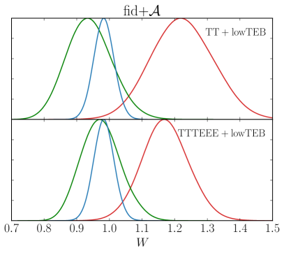
Constraints on from these two data sets are shown in
Fig. 15 (top).
Comparing these two constraints leads to a tension of 2.4, the same as the
model-independent tension derived in the previous section. When adding polarization data,
the tension evaluates to the same 2.4, slightly more than the model-independent
value; see Fig. 15 for changes in the posteriors.
Comparing instead constraints on directly leads to the same tension
significance both with and without polarization. The good agreement with constraints on
gives further evidence that is a powerful and robust tension indicator,
even though it is constructed from
a single PC.
With we can also compare the predictions from the unlensed parameters
in the same fid+ context.
These correspond to the green curves in
Fig. 15 and when compared with their red counterparts evaluate to
internal tensions significant at 2.4 for TT+lowTEB, respectively
2.1 for TTTEEE+lowTEB.
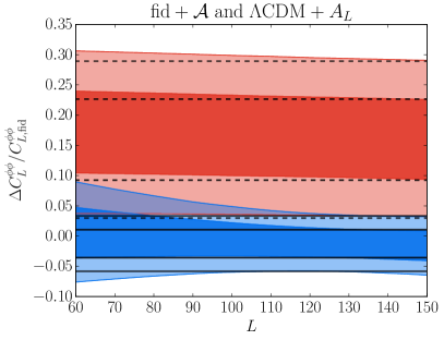
Within the fid+ model considered here, constraints on any show the same significance of the tension as (see Fig. 16, solid vs. dashed lines). Nonetheless, there are subtleties in using itself as a tension indicator beyond , even for parameterizations that are motivated by CDM. As we argued above, to quote tension in measurements, one has to exactly specify how much freedom in the lensing potential is allowed; in the PC case, this turns into a sensitivity to the number of PCs involved.
For variations motivated by CDM, one has to carefully specify which parameters
are allowed to independently vary between the reconstruction and CMB power spectra
analyses.
For example, let us take the case of comparing the temperature power spectrum
TT+lowT
and lens reconstruction measurements as commonly considered in the literature. For the former case we further
take the usual CDM+ approach which allows some variation in the
shape of the lensing power spectrum through the cosmological parameters.
Without the low- polarization data,
we must specify the prior on since it controls through the
measured amplitude of the temperature peaks.
For definiteness let us take
a Gaussian prior of .
Given reconstruction data alone, CDM allows both amplitude and larger shape changes since the cosmological parameters are not constrained by CMB power spectra. For definiteness, let us take the joint posterior of the CDM parameters with Gaussian priors and . Constraints on when allowing these variations are shown in Fig. 16 (red vs. blue contours). Note that as decreases, these additional shape variations in weaken the apparent tension.
When one compares constraints on , this is the technique used in Ref. Aghanim et al. (2017)*7*7*7Marius Millea, private communication. At the shape variation only has a mild effect that is further reduced by the shift in both contours so for we retain a tension significance of 2.4.*8*8*8The small difference from the value 2.3 quoted in Ref. Aghanim et al. (2017) can be caused by different analysis choices.
At lower the shape variations become more important.
On the lensing reconstruction side, the CDM parameters are not
well constrained and allow values that are inconsistent with the unlensed CMB; this
leads to the shape variations noticeable at low in Fig. 16.
Had we allowed even larger freedom
in by changing say the prior on on the reconstruction side, the apparent
tension would further degrade.
On the TT+lowT side the CDM parameters are very well constrained,
leaving less of an effect on the shape of and the contours mostly reflect
uncertainty in the amplitude through .
However, when more freedom is granted to the lensing potential, the apparently
strong constraints at low degrade (see Fig. 7), also decreasing
the tension.
It is thus important to carefully specify the model freedom
in using as a statistic. This problem is largely removed by using
which has the same meaning in all models.
V Discussion
In this work we separate the lensing information from CMB power spectra from the cosmological parameters that control the high redshift physics and thereby illuminate the so-called “lensing tensions” in the Planck CMB data. By modeling the principal components of the lens potential given the Planck CMB power spectra, we isolate the one aspect that is constrained by the data in a model independent way. We then compare this constraint to results from lens reconstruction through the 4 principal components that it constraints to test whether variations in beyond CDM can relax tension between the two different sources of lensing information.
We show that the tension remains between the temperature and lensing reconstruction determinations of even beyond CDM. Previous studies of the Planck lensing anomaly Ade et al. (2016c); Aghanim et al. (2017); Addison et al. (2016); Ade et al. (2014) considered only the addition of changes in the amplitude of the gravitational lensing potential from CDM predictions. Our technique extends these studies and clarifies the nature of the tension by extracting direct constraints on , which obviates the need for directly specifying CDM parameters in interpreting tension, and allowing shape variations from CDM.
Even allowing for shape and amplitude variations beyond CDM, the tension between temperature and lensing reconstruction remains at a level of 2.4, essentially the same as with amplitude variations alone. The significance decreases mildly to 2.2 when polarization data are taken into account unlike in the case of amplitude variations; this drop is driven by preference of the TE data for less lensing.
We evaluate these tension significances x by using a simple difference of the means statistic tension on a simple function of the first principal component. For the Planck 2015 data which measure only a single aspect of lensing from CMB power spectra, this provides a simple but powerful, robust, and lensing model independent quantification of tension. Our technique can be easily applied to future CMB data sets, where more and mutually correlated aspects are measured Motloch et al. (2017); Motloch and Hu (2017), with a suitable generalization of tension statistics (e.g. Kullback and Leibler (1951)).
This tension is driven by the multipole range in the TT data which prefers smoother acoustic peaks than predicted by the standard physics at recombination and lensing reconstruction. While new physics at recombination could in principle relieve tension, it cannot be relieved by adjusting the relativistic degrees of freedom through .
By separating information in the lensed CMB power spectra into lensing and unlensed components, we also enable a consistency check on the CDM cosmological model. Because the CDM prediction based on constraints to the unlensed CMB is consistent with the lensing reconstruction constraints, the internal consistency check fails at similar significance as the comparison of the temperature – lensing reconstruction determinations of lensing potential. Addition of polarization data again decreases the significance of the tension, more so this time due to preference for high in the TE data.
While these tensions may point to systematic errors or a statistical fluke that is resolved by more data and improved data reduction, our technique of extracting direct constraints on the lensing potential from CMB power spectra data should continue to provide a robust and powerful tool for testing the consistency of CDM and searching for new physics in the future.
Acknowledgements.
We thank Niayesh Afshordi, Neal Dalal, Marius Millea and Marco Raveri for useful discussions. This work was supported by NASA ATP NNX15AK22G and the Kavli Institute for Cosmological Physics at the University of Chicago through grant NSF PHY-1125897 and an endowment from the Kavli Foundation and its founder Fred Kavli. WH was additionally supported by U.S. Dept. of Energy contract DE-FG02-13ER41958 and the Simons Foundation. We acknowledge use of the CAMB and CosmoMC software packages. This work was completed in part with resources provided by the University of Chicago Research Computing Center. PM thanks the Perimeter Institute for Theoretical Physics where part of this work was performed. Research at Perimeter Institute is supported by the Government of Canada through the Department of Innovation, Science and Economic Development and by the Province of Ontario through the Ministry of Research and Innovation.References
- Lewis and Challinor (2006) A. Lewis and A. Challinor, Phys. Rept. 429, 1 (2006), arXiv:astro-ph/0601594 [astro-ph] .
- Smith et al. (2007) K. M. Smith, O. Zahn, and O. Dore, Phys. Rev. D76, 043510 (2007), arXiv:0705.3980 [astro-ph] .
- Hirata et al. (2008) C. M. Hirata, S. Ho, N. Padmanabhan, U. Seljak, and N. A. Bahcall, Phys. Rev. D 78, 043520 (2008).
- Hanson et al. (2013) D. Hanson et al. (SPTpol), Phys. Rev. Lett. 111, 141301 (2013), arXiv:1307.5830 [astro-ph.CO] .
- Das et al. (2011) S. Das et al., Phys. Rev. Lett. 107, 021301 (2011), arXiv:1103.2124 [astro-ph.CO] .
- Keisler et al. (2011) R. Keisler et al., Astrophys. J. 743, 28 (2011), arXiv:1105.3182 [astro-ph.CO] .
- Ade et al. (2014) P. A. R. Ade et al. (The Planck Collaboration), Astron. & Astrophys. 571, A17 (2014), arXiv:1303.5077 .
- Keisler et al. (2015) R. Keisler et al. (SPT), Astrophys. J. 807, 151 (2015), arXiv:1503.02315 [astro-ph.CO] .
- Ade et al. (2016a) P. A. R. Ade et al. (Planck), Astron. Astrophys. 594, A15 (2016a), arXiv:1502.01591 [astro-ph.CO] .
- Ade et al. (2016b) P. A. R. Ade et al. (BICEP2, Keck Array), (2016b), arXiv:1606.01968 [astro-ph.CO] .
- Sherwin et al. (2016) B. D. Sherwin et al., ArXiv e-prints (2016), arXiv:1611.09753 .
- Seljak (1996) U. Seljak, Astrophys. J. 463, 1 (1996), arXiv:astro-ph/9505109 [astro-ph] .
- Zaldarriaga (2000) M. Zaldarriaga, Phys. Rev. D62, 063510 (2000), arXiv:astro-ph/9910498 [astro-ph] .
- Hu (2001) W. Hu, Phys. Rev. D64, 083005 (2001), arXiv:astro-ph/0105117 [astro-ph] .
- Hu and Okamoto (2002) W. Hu and T. Okamoto, Astrophys. J. 574, 566 (2002), arXiv:astro-ph/0111606 [astro-ph] .
- Okamoto and Hu (2003) T. Okamoto and W. Hu, Phys. Rev. D67, 083002 (2003), arXiv:astro-ph/0301031 [astro-ph] .
- Hirata and Seljak (2003) C. M. Hirata and U. Seljak, Phys. Rev. D68, 083002 (2003), arXiv:astro-ph/0306354 [astro-ph] .
- Smith et al. (2012) K. M. Smith, D. Hanson, M. LoVerde, C. M. Hirata, and O. Zahn, JCAP 1206, 014 (2012), arXiv:1010.0048 [astro-ph.CO] .
- Ade et al. (2016c) P. A. R. Ade et al. (Planck), Astron. Astrophys. 594, A13 (2016c), arXiv:1502.01589 [astro-ph.CO] .
- Aghanim et al. (2017) N. Aghanim et al. (Planck), Astron. Astrophys. 607, A95 (2017), arXiv:1608.02487 [astro-ph.CO] .
- Addison et al. (2016) G. E. Addison, Y. Huang, D. J. Watts, C. L. Bennett, M. Halpern, G. Hinshaw, and J. L. Weiland, Astrophys. J. 818, 132 (2016), arXiv:1511.00055 [astro-ph.CO] .
- Ade et al. (2014) P. A. R. Ade et al. (Planck), Astron. Astrophys. 571, A16 (2014), arXiv:1303.5076 [astro-ph.CO] .
- Carron et al. (2017) J. Carron, A. Lewis, and A. Challinor, JCAP 1705, 035 (2017), arXiv:1701.01712 [astro-ph.CO] .
- Motloch et al. (2017) P. Motloch, W. Hu, and A. Benoit-Lévy, Phys. Rev. D95, 043518 (2017), arXiv:1612.05637 [astro-ph.CO] .
- Motloch and Hu (2017) P. Motloch and W. Hu, (2017), arXiv:1709.03599 [astro-ph.CO] .
- Lewis and Bridle (2002) A. Lewis and S. Bridle, Phys. Rev. D66, 103511 (2002), arXiv:astro-ph/0205436 [astro-ph] .
- Gelman and Rubin (1992) A. Gelman and D. B. Rubin, Statist. Sci. 7, 457 (1992).
- Smith et al. (2006) K. M. Smith, W. Hu, and M. Kaplinghat, Phys. Rev. D74, 123002 (2006), arXiv:astro-ph/0607315 [astro-ph] .
- Adam et al. (2016) R. Adam et al. (Planck), Astron. Astrophys. 596, A108 (2016), arXiv:1605.03507 [astro-ph.CO] .
- Benoit-Levy et al. (2012) A. Benoit-Levy, K. M. Smith, and W. Hu, Phys. Rev. D86, 123008 (2012), arXiv:1205.0474 [astro-ph.CO] .
- Obied et al. (2017) G. Obied, C. Dvorkin, C. Heinrich, W. Hu, and V. Miranda, Phys. Rev. D96, 083526 (2017), arXiv:1706.09412 [astro-ph.CO] .
- Riess et al. (2018) A. G. Riess, S. Casertano, W. Yuan, L. Macri, J. Anderson, J. W. MacKenty, J. B. Bowers, K. I. Clubb, A. V. Filippenko, D. O. Jones, and B. E. Tucker, Astrophys. J. 855, 136 (2018), arXiv:1801.01120 [astro-ph.SR] .
- Hu and Holder (2003) W. Hu and G. P. Holder, Phys. Rev. D68, 023001 (2003), arXiv:astro-ph/0303400 [astro-ph] .
- Heinrich et al. (2016) C. H. Heinrich, V. Miranda, and W. Hu, (2016), arXiv:1609.04788 [astro-ph.CO] .
- Kullback and Leibler (1951) S. Kullback and R. A. Leibler, Ann. Math. Statist. 22, 79 (1951).