Quantum-Mechanical Relation between Atomic Dipole Polarizability
and the van der Waals Radius

Abstract

The atomic dipole polarizability, $\alpha$, and the van der Waals (vdW) radius, $R_{\rm vdW}$, are two key quantities to describe vdW interactions between atoms in molecules and materials. Until now, they have been determined independently and separately from each other. Here, we derive the quantum-mechanical relation $R_{\rm vdW}=const.\times\alpha^{\nicefrac{{1}}{{7}}}$ which is markedly different from the common assumption $R_{\rm vdW}\propto\alpha^{\nicefrac{{1}}{{3}}}$ based on a classical picture of hard-sphere atoms. As shown for 72 chemical elements between hydrogen and uranium, the obtained formula can be used as a unified definition of the vdW radius solely in terms of the atomic polarizability. For vdW-bonded heteronuclear dimers consisting of atoms $A$ and $B$, the combination rule $\alpha=(\alpha_{A}+\alpha_{B})/2$ provides a remarkably accurate way to calculate their equilibrium interatomic distance. The revealed scaling law allows to reduce the empiricism and improve the accuracy of interatomic vdW potentials, at the same time suggesting the existence of a non-trivial relation between length and volume in quantum systems.

The idea to use a specific radius, describing a distance an atom maintains from other atoms in non-covalent interactions, was introduced by Mack Mack1932 and Magat Magat1932 . Subsequently, it was employed by Kitaigorodskii in his theory of close packing of molecules in crystals Kitaigorodskii1955 ; Kitaigorodskii1971 . This opened a wide area of applications related to the geometrical description of non-covalent bonds Zefirov1989 ; Zefirov1995 . The currently used concept of the vdW radius was formalized by Pauling Pauling1960 and Bondi Bondi1964 , who directly related it to vdW interactions establishing its current name. They defined this radius as half of the distance between two atoms of the same chemical element, at which Pauli exchange repulsion and London dispersion attraction forces exactly balance each other. Since then, together with the atomic dipole polarizability, the vdW radius serves for atomistic description of vdW interactions in many fields of science including molecular physics, crystal chemistry, nanotechnology, structural biology, and pharmacy.

The atomic dipole polarizability, a quantity related to the strength of the dispersion interaction, can be accurately determined from both experiment and theory to an accuracy of a few percent for most elements in the periodic table Chu2004 ; Tkatchenko2009 ; Tkatchenko2012 ; Gobre2016 ; Gould2016 ; Hermann2017 . In contrast, the determination of the atomic vdW radius is unambiguous for noble gases only, for which the vdW radius is defined as half of the equilibrium distance in the corresponding vdW-bonded homonuclear dimer Pauling1960 ; Bondi1964 . For other chemical elements, the definition of vdW radius requires the consideration of molecular systems where the corresponding atom exhibits a closed-shell behavior similar to noble gases, in order to distinguish the vdW bonding from other interactions Zefirov1989 ; Zefirov1995 . Hence, a robust determination of vdW radii for most elements in the periodic table requires a painstaking analysis of a substantial amount of experimental structural data Batsanov2001 .

Consequently, from an experimental point of view, the vdW radius can only be considered as a statistical quantity and available databases provide just recommended values. Among them, the one proposed in 1964 by Bondi Bondi1964 has been extensively used. However, it is based on a restricted amount of experimental information available at that time. With the improvement of experimental techniques and increase of available data, it became possible to derive more precise databases. A comprehensive analysis was performed by Batsanov Batsanov2001 . He provided a table of accurate atomic vdW radii for 65 chemical elements serving here as a benchmark reference Comment_1 . For noble gases, missing in Ref. Batsanov2001 , the vdW radii of Bondi Bondi1964 are taken in our analysis Comment_2 . As a reference dataset for the atomic dipole polarizability, we use Table A.1 of Ref. Gobre2016 . They are obtained with time-dependent density-functional theory and linear-response coupled-cluster calculations providing an accuracy of a few percent, which is comparable to the variation among different sets of experimental and theoretical results Gould2016 .

The commonly used relation between the atomic dipole polarizability and the vdW radius is based on a classical approach, wherein an atom is described as a positive point charge $q$ compensated by a uniform electron density $(-3q)/(4\pi R_{\rm a}^{3})$ within a hard sphere. Its radius $R_{\rm a}$ is identical to the classical vdW radius. With an applied electric field $\mathcal{E}_{\rm ext}$, the point charge undergoes a displacement $d$ with respect to the center of the sphere. From the force balance, $q\mathcal{E}_{\rm ext}-q^{2}d/R_{\rm a}^{3}=0$, and the definition of the dipole polarizability via the induced dipole moment, $qd=\alpha\mathcal{E}_{\rm ext}$, it follows that

$$\begin{array}[]{ll}R_{\rm a}=\alpha^{\nicefrac{{1}}{{3}}}\ .\end{array}$$ (2)

This scaling law is widely used in literature relating the vdW radius to the polarizability.

In this Letter, we show that the quantum-mechanical (QM) relation between the two quantities is markedly different from the classical formula. This result is obtained from the force balance between vdW attraction and exchange-repulsion interactions considered within a simplified, yet realistic, QM model. Our finding is supported by a detailed analysis of robust data for atomic polarizabilities and vdW radii of 72 chemical elements.

Table 1: For noble gases, the proportionality function of the QDO model given by Eq. (12) is shown versus its counterpart of real atoms. The results are obtained with $\mu\omega$ from Ref. Jones2013 ; Comment_3 and the reference vdW radii Bondi1964 ; Runeberg1998 and polarizabilities Gobre2016 . All values are given in atomic units.

Species	$\mu\omega$	$R_{\rm vdW}^{\rm ref}$	$\alpha^{\rm ref}$	$C(\mu\omega,R_{\rm vdW}^{\rm ref})$	$R_{\rm vdW}^{\rm ref}/(\alpha^{\rm ref})^{\nicefrac{{1}}{{7}}}$
He	0.5178	2.65	1.38	2.33	2.53
Ne	0.4526	2.91	2.67	2.56	2.53
Ar	0.2196	3.55	11.10	2.33	2.52
Kr	0.1778	3.82	16.80	2.35	2.55
Xe	0.1309	4.08	27.30	2.28	2.54
Rn	0.1092	4.23	33.54	2.25	2.56

Many properties of real atoms can be captured by physical models based on Gaussian wave functions Bloch1997 . Among them, the quantum Drude oscillator (QDO) model Wang2001 ; Sommerfeld2005 ; Jones2013 serves as an insightful, efficient, and accurate approach Tkatchenko2012 ; Reilly2015 ; Tkatchenko2015 ; Sadhukhan2016 ; Gobre2016 ; Sadhukhan2017 ; Hermann2017 for the description of the dispersion interaction. It provides the dipole polarizability $\alpha\equiv\alpha_{1}=q^{2}/\mu\omega^{2}$ expressed in terms of the three parameters Jones2013 : the charge $q$, the mass $\mu$, and the characteristic frequency $\omega$ modeling the response of valence electrons. The scaling laws obtained for dispersion coefficients within the QDO model are applicable to accurately describe attractive interactions between atoms and molecules Tkatchenko2009 ; Tkatchenko2012 ; Jones2013 ; Gobre2016 ; Hermann2017 . Here, we introduce the exchange–repulsion into this model to uncover a QM relation between the polarizability and vdW radius. Motivated by the work of Pauling Pauling1960 and Bondi Bondi1964 , we determine the latter from the condition of the balance between exchange–repulsion and dispersion–attraction forces. The modern theory of interatomic interactions Stone-book suggests that the equilibrium binding between two atoms (including noble gases) results from a complex interplay of many interactions. Among them, exchange–repulsion, electrostatics, polarization, and dipolar as well as higher-order vdW dispersion interactions are of importance. However, it is also known that the Tang-Toennies model Tang1995 ; Tang1998 ; Tang2003 , which consists purely of a dispersion attraction and an exchange repulsion, reproduces binding energy curves of closed-shell dimers with remarkable accuracy. To express the vdW radius in terms of the dipole polarizability, our initial model presented here treats the repulsive and attractive forces by employing a dipole approximation for the Coulomb potential. Such an approximation turns out to be reasonable to correctly describe the equilibrium distance for homonuclear closed-shell dimers via the condition of vanishing interatomic force. Our dipolar QM model can also be generalized to higher multipoles, as demonstrated by the excellent correlation between higher-order atomic polarizabilities and the vdW radius (see Eq. (26)).

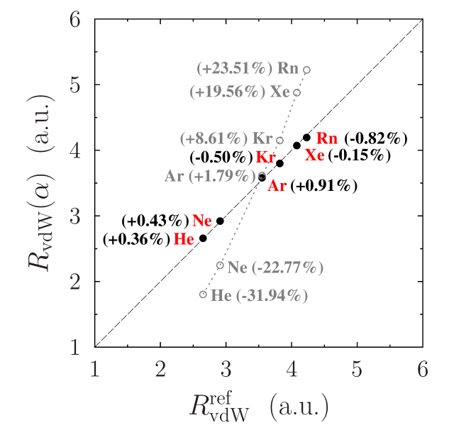
Figure 1: (Color online) The van der Waals radius obtained for noble gases by Eq. (14) is presented in comparison to its reference Batsanov2001 counterpart (black full dots). In addition, the results obtained by the fit of the classical scaling law to the reference data, $R_{\rm vdW}(\alpha)=1.62\,\alpha^{\nicefrac{{1}}{{3}}}$, are shown (grey circles). The relative errors calculated with Eq. (16) are in parentheses.

A coarse-grained QDO represents response properties of all valence electrons in an atom as those of a single oscillator Jones2013 . As a result, usual prescriptions to derive the Pauli exchange repulsion from the interaction of each electron pair Tang1998 are not straightforward within this model. However, two QDOs with the same parameters are indistinguishable. In addition, their spin-less structure Jones2013 is well suited to describe closed valence shells of atoms, which interact solely via the vdW forces. Considering two identical QDOs as bosons, we construct the total wavefunction as a permanent and introduce the exchange interaction following the Heitler-London approach Heitler1927 , where it is expressed in terms of the Coulomb and exchange integrals.

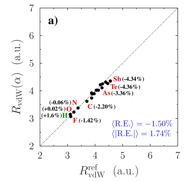
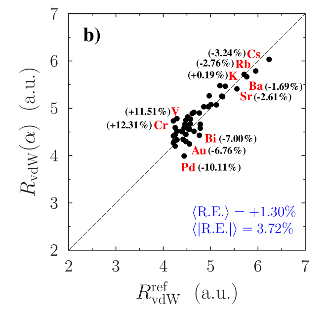
Figure 2: (Color online) The vdW radius obtained by Eq. (14) using the reference data for the polarizability Gobre2016 is shown separately for a) nonmetals/metalloids and b) metals in comparison to its reference counterpart Batsanov2001 . Here, $\langle\text{R.E.}\rangle$ and $\langle|\text{R.E.}|\rangle$ represent the mean of the relative error and its magnitude, respectively, calculated with Eq. (16) for the database of Batsanov Comment_1 . In addition, we show the comparison between $R_{\rm vdW}(\alpha)$ and $R_{\rm vdW}^{\rm ref}$ for H with the latter one taken from Ref. Tkatchenko2009 .

Let us consider a homonuclear dimer consisting of two atoms separated by the distance $R$. As shown in the Supplemental Material Supplementary , the dipole approximation for the Coulomb interaction provides the exchange integral in the simple form

$$\begin{array}[]{ll}J_{\rm ex}=\frac{q^{2}S}{2R}=\frac{q^{2}}{2R}~{}e^{-\frac{\mu\omega}{2\hbar}R^{2}}\ ,\end{array}$$ (4)

whereas the corresponding Coulomb integral vanishes. At the equilibrium distance, $R=2R_{\rm vdW}$, of homonuclear dimers consisting of the species of Table I, the overlap integral, $S$ in Eq. (4), is less than $0.02$ Supplementary . In the first-order approximation with respect to $S$, the exchange energy for the symmetric state, related to the bosonic nature of the closed shells, is given by $J_{\rm ex}$ Supplementary . As follows from Table I, for $R=2R_{\rm vdW}$, the condition $\frac{\mu\omega}{\hbar}\gg\frac{1}{R^{2}}$ is fulfilled. Then, the corresponding force, $F_{\rm ex}=-\nabla_{R}J_{\rm ex}$, can be obtained as Supplementary

$$\begin{array}[]{ll}F_{\rm ex}\approx\frac{q^{2}}{2}\frac{\mu\omega}{\hbar}~{}e^{-\frac{\mu\omega}{2\hbar}R^{2}}=\frac{\alpha\hbar\omega}{2}\left(\frac{\mu\omega}{\hbar}\right)^{2}~{}e^{-\frac{\mu\omega}{2\hbar}R^{2}}\ .\end{array}$$ (6)

The attractive dipole-dipole dispersion interaction and the related force are known within the QDO model as Jones2013

$$\begin{array}[]{ll}E_{\rm disp}=-\frac{3}{4}\frac{\alpha^{2}\hbar\omega}{R^{6}}\ \ \ \ \text{and}\ \ \ \ F_{\rm disp}=-\frac{9}{2}\frac{\alpha^{2}\hbar\omega}{R^{7}}\ ,\end{array}$$ (8)

respectively. From $F_{\rm ex}+F_{\rm disp}=0$, we get the relation

$$\begin{array}[]{ll}R_{\rm vdW}=C(\mu\omega,R_{\rm vdW})~{}\alpha^{\nicefrac{{1}}{{7}}}\ .\end{array}$$ (10)

Here, the proportionality function Comment_4

$$\begin{array}[]{ll}C(\mu\omega,R_{\rm vdW})=\frac{1}{2}\left(\frac{3\hbar}{\mu\omega}\right)^{\nicefrac{{2}}{{7}}}\exp\left({\frac{2\mu\omega R_{\rm vdW}^{2}}{7\hbar}}\right)\end{array}$$ (12)

depends on both $\mu\omega$ and $R_{\rm vdW}$. However, as shown by Table I, the deviations of $C(\mu\omega,R_{\rm vdW})$ from its mean value of 2.35 are within 9% among different species. This is in contrast to the strong variation of the model parameters by themselves. Moreover, the actual ratio $R_{\rm vdW}/(\alpha)^{\nicefrac{{1}}{{7}}}$ is practically constant for all noble-gas atoms, according to the last column in Table I. By fitting the scaling law $R_{\rm vdW}\propto(\alpha)^{\nicefrac{{1}}{{7}}}$ to the reference data for noble gases Bondi1964 ; Runeberg1998 , we obtain a remarkable relation

$$\begin{array}[]{ll}R_{\rm vdW}(\alpha)=2.54~{}\alpha^{\nicefrac{{1}}{{7}}}~{}\text{a.u.}\end{array}$$ (14)

which is the central result of our work Comment_5 .

The function $C(\mu\omega,R_{\rm vdW})$ corresponds to a universal scaling law between the atomic volume and the electron density at $R_{\rm vdW}$ Comment_4 . Its deviations from 2.54 can be attributed to the model simplifications related to the coarse-grained description of valence electrons by Gaussian wave functions.

Figure 1 shows that Eq. (14) yields a relative error

$$\begin{array}[]{ll}\text{R.E.}=\left[(R_{\rm vdW}(\alpha)-R_{\rm vdW}^{\rm ref})/R_{\rm vdW}^{\rm ref}\right]\times 100\%\end{array}$$ (16)

of less than 1% for all noble gas atoms. In contrast, the fit of the classical scaling law of Eq. (2) to the reference data is clearly unreasonable. The power law of Eq. (14) is also supported by our extended statistical analysis performed for the noble gases by assuming different possible power laws Supplementary . Among them, the one of Eq. (14) is identified as the actual scaling law with the coefficient of variation of less than 1% as well as the one with the minimal standard deviation.

Let us now assess the validity of the relation given by Eq. (14) for atoms of other chemical elements. To this end, we use the equilibrium vdW radii of Batsanov Batsanov2001 as the reference Comment_1 . For hydrogen, we take the value of the vdW radius from Ref. Tkatchenko2009 . The results of our analysis are illustrated in Fig. 2 separately for nonmetals/metalloids (16 elements of Ref. Batsanov2001 + H) and metals (49 elements). A detailed information is provided in the Supplemental Material Supplementary . We observe an excellent correlation between $R_{\rm vdW}(\alpha)$ and its reference counterpart for a wide range of input data: $1.38\leqslant\alpha^{\rm ref}\leqslant 427.12$ Gobre2016 and $2.65\leqslant R_{\rm vdW}^{\rm ref}\leqslant 6.24$. Both the mean of the relative error, $\langle\text{R.E.}\rangle$, and its magnitude, $\langle|\text{R.E.}|\rangle$, are within a few percent. Moreover, $\langle\text{R.E.}\rangle$ for the complete database of Batsanov is just 0.61%, which means that positive and negative deviations are almost equally distributed. Since the reference vdW radii are determined with a statistical error of up to 10% Batsanov2001 , these results are already enough to support the validity of Eq. (14).

The reliability of the obtained formula becomes even more evident from a further detailed analysis based on our separate treatment of the nonmetals/metalloids and metals. The experimentally based determination of $R_{\rm vdW}$ is known to be more difficult for atoms with metallic properties Batsanov2001 , because of lack of structures where they undergo vdW-bonded contacts with other molecular moieties. The transition elements are even more problematic since they exhibit a variety of possible electronic states. Therefore, going from nonmetals via metalloids and simple metals to transition metals, the statistical error increases. Figure 2 clearly demonstrates such a situation. On one hand, for the organic elements (C, N, O) the agreement is better in comparison to the metalloids (As, Sb, Te). On the other hand, the transition metals (V, Cr, Pd) show larger deviations in comparison to the simple metals (K, Rb, Sr). It is also worth mentioning that, among all the elements from the used database Comment_6 , $|\text{R.E.}|$ exceeds 10% only for V, Cr, and Pd.

An important feature of Eq. (14) is its transferability to vdW-bonded heteronuclear dimers. The equilibrium distance between two different atoms $A$ and $B$ can be obtained by the arithmetic mean

$$\begin{array}[]{ll}D_{\rm a}(\alpha)=2\times 2.54\left[(\alpha_{A}+\alpha_{B})/2\right]^{\nicefrac{{1}}{{7}}}\text{a.u.}\end{array}$$ (18)

as generalization of the equilibrium distance in homonuclear dimers, $D(\alpha)\equiv 2\times R_{\rm vdW}=2\times 2.54\,\alpha^{\nicefrac{{1}}{{7}}}$. The box plot of Fig. 3 illustrates that the simple combination rule of Eq. (18) yields accurate equilibrium distances of 15 vdW-bonded heteronuclear dimers of noble gases. The corresponding $|{\rm R.E.}|$ with respect to the reference data Tang2003 is within 2.5%, whereas $\langle{\rm R.E.}\rangle$ and $\langle|{\rm R.E.}|\rangle$ are about 0.2% and 1%, respectively Supplementary . In comparison, the other three possible combination rules based on simple means,

$$\begin{array}[]{ll}D_{\rm a}(R_{\rm vdW})=2\times\left(R_{\rm vdW}^{A}+R_{\rm vdW}^{B}\right)/2\ ,\end{array}$$ (20)

$$\begin{array}[]{ll}D_{\rm g}(\alpha)=2\times 2.54\left(\sqrt{\alpha_{A}\alpha_{B}}\right)^{\nicefrac{{1}}{{7}}}\ ,\end{array}$$ (22)

$$\begin{array}[]{ll}D_{\rm g}(R_{\rm vdW})=2\times\left(R_{\rm vdW}^{A}R_{\rm vdW}^{B}\right)^{\nicefrac{{1}}{{2}}}\ ,\end{array}$$ (24)

underestimate the equilibrium distances with $|\text{R.E.}|$ exceeding 10% and both $\langle{\rm R.E.}\rangle$ and $\langle|{\rm R.E.}|\rangle$ of about 4-5%.

Among its various possible applications, the proposed determination of the atomic vdW radius and the equilibrium distance for vdW bonds provides a powerful way to parametrize interatomic potentials. Many models, like the Lennard-Jones potential, use a geometric and an energetic parameter. The former, related to the equilibrium distance, can now be determined via the polarizability according to Eqs. (14) and (18). Since the remaining parameter corresponds to the dissociation energy, the full parametrization becomes now easily accessible by experiment. There are also models, like the modified Tang-Toennies potential Tang1995 , based just on one combined parameter, which can be now directly evaluated from the extremum condition on the known equilibrium distance.

Based on Eq. (14), one can also significantly improve the efficiency of computational models for intermolecular interactions by revising the determination of effective vdW radii of atoms in molecules. According to the classical result, the vdW radius is conventionally calculated as $R_{\rm vdW}^{\rm eff}=({\alpha^{\rm eff}}/{\alpha^{\rm free}})^{\nicefrac{{1}}{{3}}}R_{\rm vdW}^{\rm free}$ with the effective atomic polarizability obtained from the corresponding electron density Tkatchenko2009 . To apply this procedure, it is necessary to tabulate empirical free-atom vdW radii. With Eq. (14), this problem can now be overcome by a direct calculation $R_{\rm vdW}^{\rm eff}=2.54\,(\alpha^{\rm eff})^{\nicefrac{{1}}{{7}}}$. We test the effect of using this alternative definition of vdW radii for atoms in molecules on the binding energies of molecular dimers contained in the S66 database Rezac2011_1 by means of the Tkatchenko-Scheffler model Tkatchenko2009 in conjunction with DFT-PBE calculations Supplementary . With the alternative determination of $R_{\rm vdW}^{\rm eff}$ we obtain an accuracy increase of about 30%, in comparison to the conventional and more empirical computational scheme Supplementary . Hence, the use of Eq. (14) improves the accuracy of intermolecular interaction models as well as reduces their empiricism.

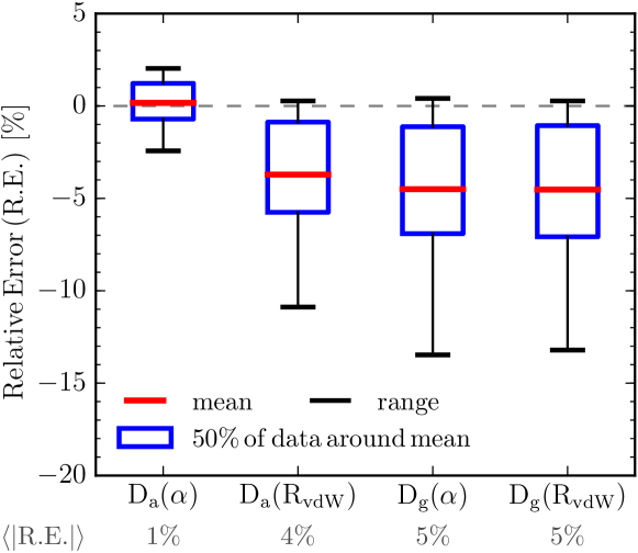
Figure 3: (Color online) Statistical analysis of the results obtained with Eqs. (18)–(24) for the equilibrium distance of 15 vdW-bonded heteronuclear dimers of noble gases (all possible pairs among He, Ne, Ar, Kr, Xe, and Rn) which is performed by comparison to the references values Tang2003 .

We have also found that Eq. (14) can be generalized to

$$\begin{array}[]{ll}R_{\rm vdW}(\alpha_{n})=C_{n}~{}\alpha_{n}^{\nicefrac{{2}}{{7(n+1)}}}\ \ ,\ \ \ n=1,2,...\end{array}$$ (26)

for the multipole polarizabilities Comment_7 . With the coefficients $C_{2}=2.45$ and $C_{3}=2.27$ as well as accurate values for $\alpha_{2}$ and $\alpha_{3}$ from Ref. Jones2013 , Eq. (26) provides $R_{\rm vdW}$ for He, Ne, Ar, Kr, and Xe within 1% and 1.4%, respectively. This indicates that higher-order attractive and repulsive forces related to each term in the Coulomb potential expansion are mutually balanced as well, which justifies the model we used to derive the scaling law of Eq. (14) Comment_8 .

In summary, the present work provides a seamless and universal definition of the vdW radius for all chemical elements solely in terms of their dipole polarizabilities, which is given by $R_{\rm vdW}(\alpha)=2.54~{}\alpha^{\nicefrac{{1}}{{7}}}$. Motivated by the definition of the vdW radius of Pauling Pauling1960 and Bondi Bondi1964 , this relation has been evaluated by using the quantum Drude oscillator model for valence electronic response. Notably, our finding implies a significant departure from the commonly employed classical scaling law, $R_{\rm vdW}\propto\alpha^{\nicefrac{{1}}{{3}}}$. In-depth analysis of the most comprehensive empirical reference radii Batsanov2001 confirms the revealed quantum-mechanical relation. Our derivation of the vdW radius dispenses with the need for its experimental determination. Moreover, the obtained relation is also successfully extended to vdW-bonded heteronuclear dimers and higher-order atomic polarizabilities. The presented results motivate future studies towards understanding the dependence of local geometric descriptors of an embedded atom on its chemical environment as well as unveiling a non-trivial relationship between length and volume in quantum-mechanical systems Comment_9 .

We acknowledge financial support from the European Research Council (ERC Consolidator Grant “BeStMo”). M. Stöhr acknowledges financial support from Fonds National de la Recherche, Luxembourg (AFR PhD Grant “CNDTEC”). We are also thankful to Dr. Igor Poltavsky for valuable discussions.

Quantum-Mechanical Relation between Atomic Dipole Polarizability
and the van der Waals Radius (Supplemental Material)
Dmitry V. Fedorov,^1,∗ Mainak Sadhukhan,¹ Martin Stöhr,¹ and Alexandre Tkatchenko^1
1Physics and Materials Science Research Unit, University of Luxembourg, L-1511 Luxembourg

Derivation of the repulsive exchange energy within the QDO model

Here, the Heitler-London approach [30] is applied to the quantum Drude oscillator model [21]. For a homonuclear dimer consisting of atoms $A$ and $B$ separated by $\mathbf{R}$, the corresponding atomic QDO wave functions are given by

$$\Psi_{A}(\mathbf{r})=\left(\frac{\mu\omega}{\pi\hbar}\right)^{\nicefrac{{3}}{{4}}}e^{-\frac{\mu\omega}{2\hbar}r^{2}}\ \ \text{and}\ \ \Psi_{B}(\mathbf{r})=\left(\frac{\mu\omega}{\pi\hbar}\right)^{\nicefrac{{3}}{{4}}}e^{-\frac{\mu\omega}{2\hbar}(\mathbf{r}-\mathbf{R})^{2}}\ ,$$

respectively. The related overlap integral is

$$S=\iint d\mathbf{r}_{1}d\mathbf{r}_{2}~{}\Psi_{A}^{*}(\mathbf{r}_{1})\Psi_{B}^{*}(\mathbf{r}_{2})\Psi_{B}(\mathbf{r}_{1})\Psi_{A}(\mathbf{r}_{2})=e^{-\frac{\mu\omega}{2\hbar}R^{2}}\ .$$

We use the dipole approximation for the Coulomb interaction

$${\hat{V}}_{\rm dip}=q^{2}\left\{\frac{[\mathbf{r}_{1}\cdot(\mathbf{r}_{2}-\mathbf{R})]}{R^{3}}-\frac{3(\mathbf{r}_{1}\cdot\mathbf{R})[(\mathbf{r}_{2}-\mathbf{R})\cdot\mathbf{R}]}{R^{5}}\right\}\ ,$$

where the origin of the coordinates $\mathbf{r}_{1}$ and $\mathbf{r}_{2}$ of the two QDOs is located on atom $A$.

Then, the corresponding Coulomb and exchange integrals are obtained as

$$C=\iint d\mathbf{r}_{1}d\mathbf{r}_{2}~{}\Psi_{A}^{*}(\mathbf{r}_{1})\Psi_{B}^{*}(\mathbf{r}_{2}){\hat{V}}_{\rm dip}\Psi_{A}(\mathbf{r}_{1})\Psi_{B}(\mathbf{r}_{2})=0$$

and

$$J_{\rm ex}=\iint d\mathbf{r}_{1}d\mathbf{r}_{2}~{}\Psi_{A}^{*}(\mathbf{r}_{1})\Psi_{B}^{*}(\mathbf{r}_{2}){\hat{V}}_{\rm dip}\Psi_{B}(\mathbf{r}_{1})\Psi_{A}(\mathbf{r}_{2})=\frac{q^{2}S}{2R}\ ,$$

respectively. We assume that the coarse-grained atomic QDO wave functions represent closed electronic shells with total zero spin. According to their bosonic nature, the dimer wave function can only be symmetric (permanent)

$$\Psi(\mathbf{r}_{1},\mathbf{r}_{2})=\frac{1}{\sqrt{2}}\left[\Psi_{A}(\mathbf{r}_{1})\Psi_{B}(\mathbf{r}_{2})+\Psi_{A}(\mathbf{r}_{2})\Psi_{B}(\mathbf{r}_{1})\right]$$

with the corresponding energy obtained as

$$E=\frac{\iint d\mathbf{r}_{1}d\mathbf{r}_{2}\Psi^{*}(\mathbf{r}_{1},\mathbf{r}_{2})\hat{H}\Psi(\mathbf{r}_{1},\mathbf{r}_{2})}{\iint d\mathbf{r}_{1}d\mathbf{r}_{2}\Psi^{*}(\mathbf{r}_{1},\mathbf{r}_{2})\Psi(\mathbf{r}_{1},\mathbf{r}_{2})}=2E_{0}+\frac{C+J_{\rm ex}}{1+S}=2E_{0}+\frac{J_{\rm ex}}{1+S}\ ,$$

where

$$\hat{H}=\hat{H}_{0}(\mathbf{r}_{1})+\hat{H}_{0}(\mathbf{r}_{2})+{\hat{V}}_{\rm dip}(\mathbf{r}_{1},\mathbf{r}_{2})$$

with

$$\hat{H}_{0}(\mathbf{r})\Psi_{A}(\mathbf{r})=E_{0}\Psi_{A}(\mathbf{r})\ \ \ \text{and}\ \ \ \hat{H}_{0}(\mathbf{r})\Psi_{B}(\mathbf{r})=E_{0}\Psi_{B}(\mathbf{r})\ .$$

At the equilibrium distance, $R=2R_{\rm vdW}$, of homonuclear dimers consisting of the species of Table I, the condition $S\ll 1$ is fulfilled:

$S_{\text{\tiny He--He}}=6.94\times 10^{-4}$ ,

$S_{\text{\tiny Ne--Ne}}=4.69\times 10^{-4}$ ,

$S_{\text{\tiny Ar--Ar}}=3.95\times 10^{-3}$ ,

$S_{\text{\tiny Kr--Kr}}=5.58\times 10^{-3}$ ,

$S_{\text{\tiny Xe--Xe}}=1.28\times 10^{-2}$ ,

$S_{\text{\tiny Rn--Rn}}=2.01\times 10^{-2}$ .

Then, neglecting the second and higher order terms with respect to the overlap integral, the repulsive exchange energy can be well approximated by

$$E_{\rm ex}\approx J_{\rm ex}=\frac{q^{2}S}{2R}=\frac{q^{2}}{2R}~{}e^{-\frac{\mu\omega}{2\hbar}R^{2}}\ .$$

The corresponding force is obtained as

$$F_{\rm ex}=-\nabla_{R}J_{\rm ex}=\frac{q^{2}}{2}\left[\frac{\mu\omega}{\hbar}+\frac{1}{R^{2}}\right]~{}e^{-\frac{\mu\omega}{2\hbar}R^{2}}\ .$$

As follows from Table I, for $R=2R_{\rm vdW}$, the condition $\frac{\mu\omega}{\hbar}\gg\frac{1}{R^{2}}$ is fulfilled. Then, one can use the following approximation

$$F_{\rm ex}\approx\frac{q^{2}}{2}\frac{\mu\omega}{\hbar}~{}e^{-\frac{\mu\omega}{2\hbar}R^{2}}=\frac{\alpha\hbar\omega}{2}\left(\frac{\mu\omega}{\hbar}\right)^{2}~{}e^{-\frac{\mu\omega}{2\hbar}R^{2}}\ ,$$

where it is taken into account that the dipole polarizability is given by $\alpha=q^{2}/\mu\omega^{2}$ within the QDO model [21].

The performed derivation is not as obvious as the more conventional approach [28] efficiently used for noble gases, which is based on the consideration of each single pair of interacting electrons. Such a detailed treatment is impossible within the coarse-grained QDO model [21], where the wave function of a single oscillator (a Drude particle) represents all valence electrons together. However, taking into account the bosonic nature of closed valence electron shells, our approach is straightforward. The validity of Eqs. (S10) and (S12) is confirmed by the reasonable agreement between the ratio $R_{\rm vdW}/\alpha^{\nicefrac{{1}}{{7}}}$ obtained either within the QDO model or with the reference data for real atoms, as demonstrated by Table I.

Extended statistical analysis for the noble gases

Here, we perform an extended statistical analysis for the six noble gases of Table I, considering the function

$$C(p,\alpha,R_{\rm vdW})=R_{\rm vdW}^{\rm ref}/(\alpha^{\rm ref})^{p}\ .$$

The reference values for the atomic dipole polarizability and the vdW radius are taken from Refs. [12] and [8,33] of the main manuscript, respectively. The following different possible power laws are assumed: $p\in\{{\nicefrac{{1}}{{3}}};{\nicefrac{{1}}{{4}}};{\nicefrac{{1}}{{5}}};{\nicefrac{{1}}{{6}}};{\nicefrac{{1}}{{7}}};{\nicefrac{{1}}{{8}}};{\nicefrac{{1}}{{9}}};{\nicefrac{{1}}{{10}}};{\nicefrac{{1}}{{100}}}\}$. We calculate the arithmetic mean

$$\langle C\rangle=\frac{1}{6}\sum\limits_{i=1}^{6}C_{i}\ \ ,$$

the standard deviation

$$\sigma=\left[\frac{1}{(6-1)}\sum\limits_{i=1}^{6}\left(C_{i}-\langle C\rangle\right)^{2}\right]^{\nicefrac{{1}}{{2}}}\ ,$$

and the coefficient of variation

$$c_{v}=\frac{\sigma}{\langle C\rangle}\times 100\%\ \ .$$

The corresponding results are shown in Table S I. Obviously, the relation between the vdW radius and the polarizability given by Eq. (7) is most reasonable among all considered power laws. The related standard deviation of 0.02 is the minimal one and the coefficient of variation is less than 1%. The other assumed relations do not provide such a good statistical picture. These results serve as an additional confirmation of the obtained scaling law solely from the statistical analysis of the reference data.

Table SI: Results of the extended statistical analysis for the noble gases (He, Ne, Ar, Kr, Xe, and Rn).

$p$	$\nicefrac{{1}}{{3}}$	$\nicefrac{{1}}{{4}}$	$\nicefrac{{1}}{{5}}$	$\nicefrac{{1}}{{6}}$	$\mathbf{\nicefrac{{1}}{{7}}}$	$\nicefrac{{1}}{{8}}$	$\nicefrac{{1}}{{9}}$	$\nicefrac{{1}}{{10}}$	$\nicefrac{{1}}{{100}}$
$\langle C\rangle$	1.71	2.02	2.24	2.41	2.54	2.64	2.73	2.80	3.46
$\sigma$	0.44	0.28	0.16	0.07	0.02	0.07	0.12	0.17	0.58
$c_{v}$	25.51%	13.92%	7.15%	2.75%	0.65%	2.75%	4.50%	5.90%	16.85%

Dependence of the obtained results on the reference polarizability

In the main manuscript, we used the atomic dipole polarizability from Table A.1 of Ref. [12], as the reference dataset. Here, Fig. S 1 shows the results obtained with $\alpha$ taken from the benchmark “Dataset for All Neutral Atoms” of Ref. [14]. Comparing it to Fig. 2, the mean of the relative error, $\langle{\rm R.E.}\rangle$, and its magnitude, $\langle|{\rm R.E.}|\rangle$, are pratically the same. This is caused by the fact that $\alpha$ is a well-determined quantity [9-14]. A remarkable difference is present only for Pd where R.E. changes from -10.11% to 3.07%. However, as discussed in the main manuscript, the values of $R_{\rm vdW}^{\rm ref}$ for transition metals are not well reliable, to judge which from the two polarizabilities for Pd is more accurate. Moreover, for organic elements corresponding to the most robust values of $R_{\rm vdW}^{\rm ref}$, the agreement with the reference vdW radius becomes slightly worse in comparison to Fig. 2. In addition to Fig. S 1, Table S II provides a more detailed information about the used reference data as well as the results obtained for $R_{\rm vdW}(\alpha)$.

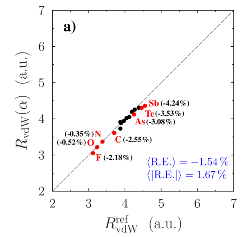
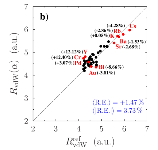
Figure S1: (Color online) The vdW radius obtained with Eq. (7) by using the reference data for the polarizability from Ref. [14] is shown separately for a) nonmetals/metalloids and b) metals in comparison to its reference counterpart [15]. Here, $\langle\text{R.E.}\rangle$ and $\langle|\text{R.E.}|\rangle$ represent the mean of the relative error and its magnitude, respectively, calculated with Eq. (8) taking $R_{\rm vdW}^{\rm ref}$ from the database of Batsanov [16].

Based on the analysis of the obtained results, we conclude that the choice of the reference dipole polarizability between two available databases plays no role for our conclusions made in the main manuscript.

Equilibrium distance in heteronuclear dimers of noble gases

As complementary to Fig. 3 of the main manuscript, Fig. S 2 and Table S III present more detailed results for the equilibrium distance in vdW-bonded heteronuclear dimers of noble gases obtained with Eqs. (9)–(12). In principle, Eqs. (11) and (12) are equivalent, since

$$2.54\,(\sqrt{\alpha_{A}\alpha_{B}})^{\nicefrac{{1}}{{7}}}=\sqrt{R_{\rm vdW}^{A}R_{\rm vdW}^{B}}\ ,$$

according to Eq. (7). The present tiny differences between the related results are caused by errors in the reference data for the vdW radii and the polarizabilities. In comparison to Eqs. (11) and (12), the results obtained with Eq. (10) are slightly more accurate. Taking into account that Eqs. (10) and (12) are the two approximations often used in literature, we can judge that the approach based on the arithmetic mean for the vdW radii is preferable. The related formula can be used for reasonable estimations of the equilibrium distance providing the relative error within 10%. However, Eq. (9), as the generalization of Eq. (7), provides much more accurate results with ${\rm R.E.}$ within 2.5%, $\langle{\rm R.E.}\rangle$ = 0.2% and $\langle|{\rm R.E.}|\rangle=1\%$.

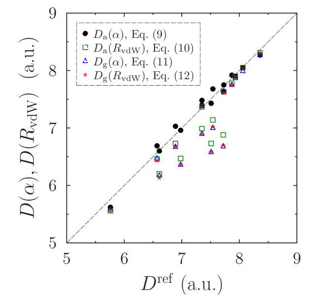
Figure S2: (Color online) The equilibrium distance of 15 vdW-bonded heteronuclear dimers of the noble gases (all possible pairs between He, Ne, Ar, Kr, Xe, and Rn) calculated with Eqs. (9)–(12) versus its reference counterpart [29].

Calculation of the effective atomic vdW radius in molecules

Here, we present detailed numerical results of our test calculations performed for molecular dimers from the S66 database [37] by means of the Tkatchenko-Scheffler (TS) method [10] with the Perdew-Burke-Ernzerhof (PBE) exchange-correlation functional [43]. The absolute and relative error of the interaction energy with respect to the coupled-cluster reference data [38] are obtained either with the old

$$R_{\rm vdW}^{\rm eff}=\left(\alpha^{\rm eff}/\alpha^{\rm free}\right)^{\nicefrac{{1}}{{3}}}R_{\rm vdW}^{\rm free}=\left(V^{\rm eff}/V^{\rm free}\right)^{\nicefrac{{1}}{{3}}}R_{\rm vdW}^{\rm free}$$

or new

$$R_{\rm vdW}^{\rm eff}=2.54\left(\alpha^{\rm eff}\right)^{\nicefrac{{1}}{{7}}}$$

way to calculate the effective atomic vdW radius in molecules. Here, the polarizability/volume ratio is obtained by means of the Hirshfeld partitioning of the electron density [10].

Similar to the approach of Ref. [10], we refitted the TS damping parameter $s_{R}$ employing Eq. (S19) on the S22 benchmark set of molecular dimers [44]. With its new value of $0.91$, in comparison to $0.94$ [10] obtained with the old scheme based on Eq. (S18), we perform our test calculations on the S66 dataset [37,38]. The corresponding density-functional calculations have been carried out using the all-electron code FHI-aims [45] with tight defaults.

As demonstrated by Table S IV, the new approach provides better accuracy for 57 from 66 molecular dimers. For nine other systems, the difference between the absolute errors related to the two approaches is still much less than the chemical accuracy (1 kcal/mol). Therefore, we may conclude that Eq. (S19) provides a general improvement of the used procedure. The mean relative error and its magnitude change from $-$11.5% to $-$7.4% and from 12.0% to 8.8%, respectively, by using the new approach instead of the old one. This corresponds to the accuracy improvement by about 30%.

This finding provides an additional confirmation of the revealed scaling law pointing out to a quite non-trivial quantum-mechanical relation between the atomic volume and the vdW radius.

Symmetry-adapted perturbation theory analysis

With the symmetry-adapted perturbation theory (SAPT) decomposition, one obtains six contributions: electrostatic ($E_{\rm pol}^{(1)}$), exchange ($E_{\rm exch}^{(1)}$), induction ($E_{\rm ind}^{(2)}$), exchange-induction ($E_{\rm exch-ind}^{(2)}$), dispersion ($E_{\rm disp}^{(2)}$), and exchange-dispersion ($E_{\rm exch-disp}^{(2)}$). In the case of neutral systems, the net induction interaction ($E_{\rm ind}^{(2)}+E_{\rm exch-ind}^{(2)}$) is almost zero due to the balance between its constituents [46] and the decomposition can be restricted to the four other contributions. For noble gas dimers, numerical results of the SAPT based on coupled-cluster approach with single and double excitations (CCSD) were provided recently in Ref. [47]. The authors have shown that their calculations are in good agreement with corresponding density-functional theory (DFT) based SAPT approaches. By using their data, we evaluate the SAPT contributions to attractive and repulsive forces for He-He, Ne-Ne, Ar-Ar, and Kr-Kr dimers considered in Ref. [47]. The magnitude of corresponding contributions is obtained within the following spans: $0.15<F_{\rm pol}^{(1)}/F_{\rm exch}^{(1)}<0.35$, $0.65<F_{\rm disp}^{(2)}/F_{\rm exch}^{(1)}<0.82$, and $0.05<F_{\rm exch-disp}^{(2)}/F_{\rm exch}^{(1)}<0.13$, where the maximal contribution $F_{\rm exch}^{(1)}$ is chosen as a reference. The net induction force ($F_{\rm ind}^{(2)}+F_{\rm exch-ind}^{(2)}$) is one order of magnitude less than $F_{\rm exch-disp}^{(2)}$ and therefore can be disregarded. This analysis shows that the force stemming from the electrostatic interaction has a relevant contribution. However, by its definition (for instance, Eq. (1) in Ref. [48]), $E_{\rm pol}^{(1)}$ is equal to the Coulomb integral which, like our Eq. (S4), vanishes in the dipole approximation for spherically symmetric atomic electron densities. Therefore, the corresponding force can contribute only for higher-order terms in multipole expansion of the Coulomb potential. Its influence needs to be considered for derivation of the general relationship given by Eq. (13), but it is irrelevant for our derivation of the scaling law expressed by Eq. (7).

Table SII: The van der Waals radius calculated according to Eq. (7) with the atomic dipole polarizability taken either from Ref. [12] ($\alpha^{(1)}$) or from Ref. [14] ($\alpha^{(2)}$) is presented in comparison to its reference [15] counterpart. The relative error (${\rm R.E.}$) is calculated by Eq. (8). A comment: for Th and U, there are no data in Ref. [14].

Species	$R_{\rm vdW}^{\rm ref}$	$\alpha^{(1)}$	$R_{\rm vdW}(\alpha^{(1)})$	${\rm R.E.}$	$\alpha^{(2)}$	$R_{\rm vdW}(\alpha^{(2)})$	${\rm R.E.}$
Li	4.9700	164.2000	5.2640	$+$5.92%	164.00	5.2631	$+$5.90%
Be	4.2141	38.0000	4.2709	$+$1.35%	37.70	4.2660	$+$1.23%
B	3.8739	21.0000	3.9239	$+$1.29%	20.50	3.9105	$+$0.94%
C	3.7039	12.0000	3.6225	$-$2.20%	11.70	3.6094	$-$2.55%
N	3.3826	7.4000	3.3807	$-$0.06%	7.25	3.3709	$-$0.35%
O	3.2314	5.4000	3.2319	$+$0.02%	5.20	3.2146	$-$0.52%
F	3.1180	3.8000	3.0737	$-$1.42%	3.60	3.0500	$-$2.18%
Na	5.2345	162.7000	5.2571	$+$0.43%	163.00	5.2585	$+$0.46%
Mg	4.5731	71.0000	4.6698	$+$2.11%	71.40	4.6736	$+$2.20%
Al	4.5353	60.0000	4.5589	$+$0.52%	57.50	4.5312	$-$0.09%
Si	4.2708	37.0000	4.2546	$-$0.38%	37.00	4.2546	$-$0.38%
P	4.0440	25.0000	4.0229	$-$0.52%	24.80	4.0183	$-$0.64%
S	3.8928	19.6000	3.8855	$-$0.19%	19.50	3.8826	$-$0.26%
Cl	3.8739	15.0000	3.7398	$-$3.46%	14.70	3.7290	$-$3.74%
K	5.7070	292.9000	5.7177	$+$0.19%	290.00	5.7096	$+$0.05%
Ca	5.2534	160.0000	5.2446	$-$0.17%	160.00	5.2446	$-$0.17%
Sc	4.9511	120.0000	5.0334	$+$1.66%	123.00	5.0512	$+$2.02%
Ti	4.6109	98.0000	4.8898	$+$6.05%	102.00	4.9179	$+$6.66%
V	4.2897	84.0000	4.7833	$+$11.51%	87.30	4.8098	$+$12.12%
Cr	4.2141	78.0000	4.7330	$+$12.31%	78.40	4.7364	$+$12.40%
Mn	4.2519	63.0000	4.5907	$+$7.97%	66.80	4.6293	$+$8.88%
Fe	4.2897	56.0000	4.5141	$+$5.23%	60.40	4.5632	$+$6.38%
Co	4.2519	50.0000	4.4416	$+$4.46%	53.90	4.4896	$+$5.59%
Ni	4.2141	48.0000	4.4158	$+$4.79%	48.40	4.4211	$+$4.91%
Cu	4.2897	42.0000	4.3324	$+$1.00%	41.70	4.3280	$+$0.89%
Zn	4.2330	40.0000	4.3023	$+$1.64%	38.40	4.2773	$+$1.05%
Ga	4.5542	60.0000	4.5589	$+$0.10%	52.10	4.4678	$-$1.90%
Ge	4.3842	41.0000	4.3175	$-$1.52%	40.20	4.3054	$-$1.80%
As	4.2519	29.0000	4.1091	$-$3.36%	29.60	4.1212	$-$3.08%
Se	4.1196	25.0000	4.0229	$-$2.35%	26.20	4.0499	$-$1.69%
Br	3.9684	20.0000	3.8967	$-$1.81%	21.60	3.9398	$-$0.72%
Rb	5.9526	319.2000	5.7884	$-$2.76%	317.00	5.7827	$-$2.86%
Sr	5.5558	199.0000	5.4106	$-$2.61%	198.00	5.4067	$-$2.68%
Y	5.1212	126.7370	5.0728	$-$0.94%	163.00	5.2585	$+$2.68%
Zr	4.8566	119.9700	5.0332	$+$3.64%	112.00	4.9840	$+$2.62%
Nb	4.6487	101.6030	4.9151	$+$5.73%	97.90	4.8891	$+$5.17%
Mo	4.5164	88.4225	4.8185	$+$6.69%	87.10	4.8082	$+$6.46%
Tc	4.4787	80.0830	4.7508	$+$6.08%	79.60	4.7467	$+$5.99%
Ru	4.4787	65.8950	4.6203	$+$3.16%	72.30	4.6819	$+$4.54%
Rh	4.3842	56.1000	4.5153	$+$2.99%	66.40	4.6253	$+$5.50%
Pd	4.4409	23.6800	3.9919	$-$10.11%	61.70	4.5771	$+$3.07%
Ag	4.4787	50.6000	4.4492	$-$0.66%	46.20	4.3918	$-$1.94%
Cd	4.4787	39.7000	4.2977	$-$4.04%	46.70	4.3985	$-$1.79%
In	4.7810	70.2200	4.6625	$-$2.48%	62.10	4.5813	$-$4.18%
Sn	4.6487	55.9500	4.5136	$-$2.91%	60.00	4.5589	$-$1.93%
Sb	4.5542	43.6719	4.3566	$-$4.34%	44.00	4.3613	$-$4.24%
Te	4.4598	37.6500	4.2652	$-$4.36%	40.00	4.3023	$-$3.53%
I	4.1952	35.0000	4.2210	$+$0.62%	33.60	4.1965	$+$0.03%
Cs	6.2361	427.1200	6.0343	$-$3.24%	396.00	5.9694	$-$4.28%
Ba	5.7637	275.0000	5.6664	$-$1.69%	278.00	5.6752	$-$1.53%
La	5.3101	213.7000	5.4659	$+$2.93%	214.00	5.4670	$+$2.95%
Hf	4.7621	99.5200	4.9006	$+$2.91%	83.70	4.7809	$+$0.39%
Ta	4.5731	82.5300	4.7713	$+$4.33%	73.90	4.6966	$+$2.70%
W	4.4598	71.0410	4.6702	$+$4.72%	65.80	4.6193	$+$3.58%
Re	4.4409	63.0400	4.5912	$+$3.38%	60.20	4.5610	$+$2.71%
Os	4.4031	55.0550	4.5032	$+$2.27%	55.30	4.5060	$+$2.34%
Ir	4.4220	42.5100	4.3399	$-$1.86%	51.30	4.4580	$+$0.81%
Pt	4.4787	39.6800	4.2974	$-$4.05%	48.00	4.4158	$-$1.40%
Au	4.5542	36.5000	4.2464	$-$6.76%	45.40	4.3808	$-$3.81%
Hg	4.2519	33.9000	4.2018	$-$1.18%	33.50	4.1947	$-$1.35%
Tl	4.7810	69.9200	4.6596	$-$2.54%	51.40	4.4592	$-$6.73%
Pb	4.7810	61.8000	4.5781	$-$4.24%	47.90	4.4145	$-$7.67%
Bi	4.7621	49.0200	4.4291	$-$6.99%	43.20	4.3499	$-$8.66%
Th	5.1967	217.0000	5.4779	$+$5.41%	—	—	—
U	5.0078	127.8000	5.0789	$+$1.42%	—	—	—

Table SIII: The equilibrium distance of 15 vdW-bonded heteronuclear dimers of the noble gases (all possible pairs between He, Ne, Ar, Kr, Xe, and Rn) calculated with Eqs. (9)–(12) in comparison to the reference values [29].

Dimer	$D^{\rm ref}$	$D_{\rm a}(\alpha)$	R.E.	$D_{\rm a}(R_{\rm vdW})$	R.E.	$D_{\rm g}(\alpha)$	R.E.	$D_{\rm g}(R_{\rm vdW})$	R.E.
He-Ne	5.76	5.62	$-$2.43%	5.56	$-$3.47%	5.58	$-$3.13%	5.55	$-$3.58%
He-Ar	6.61	6.60	$-$0.15%	6.20	$-$6.20%	6.17	$-$6.66%	6.13	$-$7.20%
He-Kr	6.98	6.96	$-$0.29%	6.47	$-$7.31%	6.36	$-$8.88%	6.36	$-$8.83%
He-Xe	7.51	7.43	$-$1.07%	6.73	$-$10.39%	6.58	$-$12.38%	6.58	$-$12.43%
He-Rn	7.72	7.64	$-$1.04%	6.88	$-$10.88%	6.68	$-$13.47%	6.70	$-$13.26%
Ne-Ar	6.57	6.69	$+$1.83%	6.46	$-$1.67%	6.47	$-$1.52%	6.43	$-$2.16%
Ne-Kr	6.89	7.03	$+$2.03%	6.73	$-$2.32%	6.67	$-$3.19%	6.67	$-$3.22%
Ne-Xe	7.35	7.48	$+$1.77%	6.99	$-$4.90%	6.90	$-$6.12%	6.89	$-$6.24%
Ne-Rn	7.54	7.68	$+$1.86%	7.14	$-$5.31%	7.00	$-$7.16%	7.02	$-$6.94%
Ar-Kr	7.35	7.40	$+$0.68%	7.37	$+$0.27%	7.38	$+$0.41%	7.37	$+$0.20%
Ar-Xe	7.73	7.75	$+$0.26%	7.63	$-$1.29%	7.64	$-$1.16%	7.61	$-$1.53%
Ar-Rn	7.87	7.92	$+$0.64%	7.78	$-$1.14%	7.75	$-$1.52%	7.75	$-$1.52%
Kr-Xe	7.93	7.90	$-$0.38%	7.90	$-$0.38%	7.87	$-$0.76%	7.90	$-$0.43%
Kr-Rn	8.06	8.05	$-$0.12%	8.05	$-$0.12%	7.99	$-$0.87%	8.04	$-$0.25%
Xe-Rn	8.36	8.27	$-$1.08%	8.31	$-$0.60%	8.27	$-$1.08%	8.31	$-$0.61%

Table SIV: Absolute (A.E. in kcal/mol) and relative (R.E.) error for the interaction energy of molecular dimers from the S66 database [37,38] obtained either with the old or new scaling law.

SYSTEM NAME	A.E. (OLD)	R.E. (OLD)	A.E. (NEW)	R.E. (NEW)	$|$A.E. (OLD)$|-|$A.E. (NEW)$|$
WaterWater	$-0.35$	$-$7.1%	$-0.30$	$-$6.1%	$+$0.05
WaterMeOH	$-0.26$	$-$4.6%	$-0.16$	$-$2.8%	$+$0.10
WaterMeNH2	$-0.96$	$-$13.7%	$-0.86$	$-$12.3%	$+$0.10
WaterPeptide	$-0.07$	$-$0.8%	$+0.06$	$+$0.7%	$+$0.00
MeOHMeOH	$-0.26$	$-$4.5%	$-0.18$	$-$3.2%	$+$0.08
MeOHMeNH2	$-1.06$	$-$14.0%	$-0.93$	$-$12.2%	$+$0.13
MeOHPeptide	$-0.33$	$-$3.9%	$-0.25$	$-$3.0%	$+$0.08
MeOHWater	$-0.31$	$-$6.2%	$-0.28$	$-$5.5%	$+$0.04
MeNH2MeOH	$-0.43$	$-$13.8%	$-0.34$	$-$10.9%	$+$0.09
MeNH2MeNH2	$-0.41$	$-$9.7%	$-0.21$	$-$4.9%	$+$0.20
MeNH2Peptide	$-0.09$	$-$1.7%	$+0.08$	$+$1.5%	$+$0.01
MeNH2Water	$-0.68$	$-$9.2%	$-0.53$	$-$7.2%	$+$0.15
PeptideMeOH	$-0.04$	$-$0.7%	$+0.10$	$+$1.6%	$-$0.06
PeptideMeNH2	$-0.71$	$-$9.4%	$-0.48$	$-$6.4%	$+$0.23
PeptidePeptide	$-0.24$	$-$2.7%	$-0.06$	$-$0.7%	$+$0.18
PeptideWater	$-0.03$	$-$0.7%	$+0.02$	$+$0.4%	$+$0.02
UracilUracilBP	$-0.19$	$-$1.1%	$-0.12$	$-$0.7%	$+$0.07
WaterPyridine	$-0.77$	$-$11.1%	$-0.68$	$-$9.8%	$+$0.09
MeOHPyridine	$-0.73$	$-$9.8%	$-0.65$	$-$8.7%	$+$0.08
AcOHAcOH	$-0.89$	$-$4.6%	$-0.82$	$-$4.2%	$+$0.07
AcNH2AcNH2	$-0.19$	$-$1.2%	$-0.09$	$-$0.5%	$+$0.10
AcOHUracil	$-0.42$	$-$2.1%	$-0.35$	$-$1.8%	$+$0.07
AcNH2Uracil	$-0.14$	$-$0.7%	$-0.05$	$-$0.2%	$+$0.09
BenzeneBenzenepipi	$-0.71$	$-$25.7%	$-0.64$	$-$23.2%	$+$0.07
PyridinePyridinepipi	$-0.70$	$-$18.4%	$-0.59$	$-$15.3%	$+$0.12
UracilUracilpipi	$+0.02$	$+$0.2%	$+0.23$	$+$2.3%	$-$0.21
BenzenePyridinepipi	$-0.73$	$-$21.6%	$-0.63$	$-$18.7%	$+$0.10
BenzeneUracilpipi	$-0.37$	$-$6.6%	$-0.19$	$-$3.4%	$+$0.18
PyridineUracilpipi	$-0.19$	$-$2.8%	$-0.02$	$-$0.2%	$+$0.17
BenzeneEthene	$-0.58$	$-$41.6%	$-0.52$	$-$37.3%	$+$0.06
UracilEthene	$-0.31$	$-$9.2%	$-0.13$	$-$3.8%	$+$0.18
UracilEthyne	$-0.07$	$-$1.8%	$+0.05$	$+$1.3%	$+$0.02
PyridineEthene	$-0.55$	$-$30.2%	$-0.45$	$-$24.6%	$+$0.10
PentanePentane	$-1.29$	$-$34.5%	$-0.86$	$-$23.0%	$+$0.43
NeopentanePentane	$-0.76$	$-$29.1%	$-0.54$	$-$20.7%	$+$0.22
NeopentaneNeopentane	$-0.66$	$-$37.8%	$-0.57$	$-$32.7%	$+$0.09
CyclopentaneNeopentane	$-0.95$	$-$39.9%	$-0.73$	$-$30.5%	$+$0.22
CyclopentaneCyclopentane	$-1.11$	$-$37.1%	$-0.80$	$-$27.0%	$+$0.30
BenzeneCyclopentane	$-0.80$	$-$22.6%	$-0.50$	$-$14.2%	$+$0.30
BenzeneNeopentane	$-0.49$	$-$17.2%	$-0.30$	$-$10.5%	$+$0.19
UracilPentane	$-0.55$	$-$11.5%	$-0.16$	$-$3.3%	$+$0.40
UracilCyclopentane	$-0.55$	$-$13.4%	$-0.23$	$-$5.7%	$+$0.32
UracilNeopentane	$-0.41$	$-$11.1%	$-0.15$	$-$4.2%	$+$0.26
EthenePentane	$-0.67$	$-$33.5%	$-0.36$	$-$18.3%	$+$0.30
EthynePentane	$-0.58$	$-$33.5%	$-0.49$	$-$28.4%	$+$0.09
PeptidePentane	$-0.73$	$-$17.3%	$-0.28$	$-$6.6%	$+$0.45
BenzeneBenzeneTS	$-0.05$	$-$1.7%	$+0.11$	$+$4.0%	$-$0.07
PyridinePyridineTS	$+0.04$	$+$1.0%	$+0.23$	$+$6.5%	$-$0.19
BenzenePyridineTS	$-0.02$	$-$0.6%	$+0.15$	$+$4.4%	$-$0.12
BenzeneEthyneCHpi	$-0.01$	$-$0.3%	$+0.11$	$+$4.0%	$-$0.10
EthyneEthyneTS	$-0.24$	$-$15.5%	$-0.19$	$-$12.6%	$+$0.04
BenzeneAcOHOHpi	$+0.10$	$+$2.2%	$+0.20$	$+$4.3%	$-$0.10
BenzeneAcNH2NHpi	$-0.07$	$-$1.7%	$+0.08$	$+$1.8%	$-$0.01
BenzeneWaterOHpi	$-0.34$	$-$10.3%	$-0.22$	$-$6.7%	$+$0.12
BenzeneMeOHOHpi	$-0.40$	$-$9.6%	$-0.25$	$-$6.0%	$+$0.15
BenzeneMeNH2NHpi	$-0.33$	$-$10.2%	$-0.18$	$-$5.5%	$+$0.15
BenzenePeptideNHpi	$-0.17$	$-$3.3%	$+0.01$	$+$0.3%	$+$0.16
PyridinePyridineCHN	$+0.45$	$+$10.7%	$+0.52$	$+$12.3%	$-$0.07
EthyneWaterCHO	$-0.14$	$-$4.9%	$-0.10$	$-$3.4%	$+$0.04
EthyneAcOHOHpi	$-0.24$	$-$4.9%	$-0.16$	$-$3.3%	$+$0.08
PentaneAcOH	$-0.73$	$-$25.2%	$-0.47$	$-$16.4%	$+$0.25
PentaneAcNH2	$-0.72$	$-$20.4%	$-0.44$	$-$12.6%	$+$0.27
BenzeneAcOH	$-0.34$	$-$8.9%	$-0.12$	$-$3.1%	$+$0.22
PeptideEthene	$-0.37$	$-$12.2%	$-0.13$	$-$4.3%	$+$0.24
PyridineEthyne	$-0.36$	$-$9.0%	$-0.29$	$-$7.2%	$+$0.07
MeNH2Pyridine	$-0.28$	$-$7.0%	$-0.09$	$-$2.3%	$+$0.19

References

- (1) E. Mack, The Spacing of Non-Polar Molecules in Crystal Lattices: The Atomic Domain of Hydrogen, J. Amer. Chem. Soc. 54, 2141 (1932).
- (2) M. Magat, Über die “Wirkungsradien” gebundener Atome und den Orthoeffekt beim Dipolmoment, Z. Phys. Chem. 16, 1 (1932).
- (3) A. I. Kitaigorodskii, Organicheskaya kristallokhimiya (Organic Crystal Chemistry), Moscow: Akad. Nauk SSSR (1955).
- (4) A. I. Kitaigorodskii, Molekulyarnye kristally (Molecular Crystals), Moscow: Nauka, 1971.
- (5) Y. V. Zefirov and P. M. Zorkii, Van der Waals Radii and Their Chemical Applications, Usp. Khim. 58, 713 (1989).
- (6) Y. V. Zefirov and P. M. Zorkii, New applications of van der Waals radii in chemistry, Russ. Chem. Rev. 64, 415 (1995).
- (7) L. Pauling, The Nature of the Chemical Bond, Ithaca: Cornell University (1960).
- (8) A. Bondi, van der Waals Volumes and Radii, J. Phys. Chem. 68, 441 (1964).
- (9) X. Chu and A. Dalgarno, Linear response time-dependent density functional theory for van der Waals coefficients, J. Chem. Phys. 121, 4083 (2004).
- (10) A. Tkatchenko and M. Scheffler, Accurate Molecular Van Der Waals Interactions from Ground-State Electron Density and Free-Atom Reference Data, Phys. Rev. Lett. 102, 073005 (2009).
- (11) A. Tkatchenko, R. A. DiStasio, Jr., R. Car, and M. Scheffler, Accurate and Efficient Method for Many-Body van der Waals Interactions, Phys. Rev. Lett. 108, 236402 (2012).
- (12) V. V. Gobre, Efficient modelling of linear electronic polarization in materials using atomic response functions, PhD thesis, Fritz Haber Institute Berlin (2016).
- (13) J. Hermann, R. A. DiStasio Jr., and A. Tkatchenko, First-Principles Models for van der Waals Interactions in Molecules and Materials: Concepts, Theory, and Applications, Chem. Rev. 117, 4714 (2017).
- (14) T. Gould and T. Bučko, Coefficients and Dipole Polarizabilities for All Atoms and Many Ions in Rows 1–6 of the Periodic Table, J. Chem. Theor. Comput. 12, 3603 (2016).
- (15) S. S. Batsanov, Van der Waals Radii of Elements, Inorganic Materials 37, 871 (2001).
- (16) In Ref. Batsanov2001 , the equilibrium vdW radius for Bi is given with an obvious misprint. Instead of Å it should be Å, which is taken into account in our analysis.
- (17) Although the vdW radii recommended for noble gases by Bondi Bondi1964 are based on old experimental data, they are quite accurate, as discussed in Ref. Mantina2009 . For Rn missing in Ref. Bondi1964 , we take the vdW radius from Ref. Runeberg1998 .
- (18) S. C. Bloch, Introduction to Classical and Quantum Harmonic Oscillators, Wiley-Interscience (1997).
- (19) F. Wang and K. D. Jordan, A Drude-model approach to dispersion interactions in dipole-bound anions, J. Chem. Phys. 114, 10717 (2001).
- (20) T. Sommerfeld and K. D. Jordan, Quantum Drude Oscillator Model for Describing the Interaction of Excess Electrons with Water Clusters: An Application to (H2O), J. Phys. Chem. A 109, 11531 (2005).
- (21) A. P. Jones, J. Crain, V. P. Sokhan, T. W. Whitfield, and G. J. Martyna, Quantum Drude oscillator model of atoms and molecules: Many-body polarization and dispersion interactions for atomistic simulation, Phys. Rev. B 87, 144103 (2013).
- (22) A. M. Reilly and A. Tkatchenko, van der Waals dispersion interactions in molecular materials: Beyond pairwise additivity, Chem. Sci. 6, 3289 (2015).
- (23) A. Tkatchenko, Current Understanding of Van der Waals Effects in Realistic Materials, Adv. Func. Mat. 25, 2054 (2015).
- (24) M. Sadhukhan and F. R. Manby, Quantum mechanics of Drude oscillators with full Coulomb interaction, Phys. Rev. B 94, 115106 (2016).
- (25) M. Sadhukhan and A. Tkatchenko, Long-Range Repulsion Between Spatially Confined van der Waals Dimers, Phys. Rev. Lett. 118, 210402 (2017).
- (26) A. Stone, The Theory of Intermolecular Forces, (Oxford University Press, 2016).
- (27) K. T. Tang, J. P. Toennies, and C. L. Yiu, Accurate Analytical He-He van der Waals Potential Based on Perturbation Theory, Phys. Rev. Lett. 74, 1546 (1995).
- (28) K. T. Tang, J. P. Toennies, and C. L. Yiu, The generalized Heitler-London theory for interatomic interaction and surface integral method for exchange energy, Int. Rev. Phys. Chem. 17, 363 (1998).
- (29) K. T. Tang and J. P. Toennis, The van der Waals potentials between all the rare gas atoms from He to Rn, J. Chem. Phys. 118, 4976 (2003).
- (30) W. Heitler and F. London, Wechselwirkung neutraler Atome und homöopolare Bindung nach der Quantenmechanik, Z. Physik 44, 455 (1927).
- (31) See Supplemental Material at http://link.aps.org/supplemental/… for detailed numerical results and other supporting information.
- (32) For Rn, missing in Ref. Jones2013 , we use the scaling law of the QDO model Jones2013 with and (a.u.) obtained in Ref. Runeberg1998 by means of relativistic pseudopotential coupled-cluster calculations.
- (33) N. Runeberg and P. Pyykkö, Relativistic Pseudopotential Calculations on Xe2, RnXe, and Rn2: The van der Waals Properties of Radon, Int. J. Quant. Chem. 66, 131 (1998).
- (34) The proportionality function can be also written as . Here, the volume is occupied by the charge density of the QDO and is its value at the vdW radius.
- (35) A strict derivation of the proportionality constant for real many-electron atoms requires additional work and it is a subject of our current studies.
- (36) In the Supplemental Material Supplementary , we show that the use of from the “Dataset for All Neutral Atoms” Gould2016 , instead of our reference values taken from Ref. Gobre2016 , does not provide remarkable changes in Fig. 2. This is valid except for Pd, where changes from -10.11% to 3.07%.
- (37) J. Řezáč, K. E. Riley, and P. Hobza, S66: A Well-balanced Database of Benchmark Interaction Energies Relevant to Biomolecular Structures, J. Chem. Theory Comput. 7, 2427 (2011);
- (38) J. Řezáč, K. E. Riley, and P. Hobza, Extensions of the S66 Data Set: More Accurate Interaction Energies and Angular-Displaced Nonequilibrium Geometries, J. Chem. Theory Comput. 7, 3466 (2011).
- (39) The multipole polarizabilities are defined as , , , and so on.
- (40) According to the symmetry-adapted perturbation theory (SAPT) decomposition Supplementary , there exists a relevant contribution to attractive forces from first-order electrostatic energy. For spherical atomic densities, this contribution vanishes within the dipole approximation used in our work Supplementary . Therefore, it is irrelevant for our current model. However, it should be taken into account for higher-order multipolar terms in the Coulomb expansion, to derive the generalized relation of Eq. (26). This task is beyond the scope of this paper and subject to ongoing investigations.
- (41) Since the atomic dipole polarizability has units of volume and is proportional to the atomic volume Tkatchenko2009 , the quantum-mechanical relation between the latter and the vdW radius becomes .
- (42) M. Mantina, A. C. Chamberlin, R. Valero, C. J. Cramer, and D. G. Truhlar, Consistent van der Waals Radii for the Whole Main Group, J. Phys. Chem. A 113, 5806 (2009).

References

- (1) [43] J. P. Perdew, K. Burke, and M. Ernzerhof, Generalized gradient approximation made simple, Phys. Rev. Lett. 77, 3865 (1996).
- (2) [44] P. Jurecka, J. Sponer, J. Cerny, and P. Hobza, Benchmark database of accurate (MP2 and CCSD(T) complete basis set limit) interaction energies of small model complexes, DNA base pairs, and amino acid pairs, Phys. Chem. Chem. Phys. 8, 1985 (2006).
- (3) [45] V. Blum, R. Gehrke, F. Hanke, P. Havu, V. Havu, X. Ren, K. Reuter, and M. Scheffler, Ab initio molecular simulations with numeric atom-centered orbitals, Comput. Phys. Commun. 180, 2175 (2009).
- (4) [46] A. Heßelmann and T. Korona, Intermolecular symmetry-adapted perturbation theory study of large organic complexes, J. Chem. Phys. 141, 094107 (2014).
- (5) [47] L. Shirkov and V. Sladek, Benchmark CCSD-SAPT study of rare gas dimers with comparison to MP-SAPT and DFT-SAPT, J. Chem. Phys. 147, 174103 (2017).
- (6) [48] A. Heßelmann, G. Jansen, and M. Schütz, Density-functional theory-symmetry-adapted intermolecular perturbation theory with density fitting: A new efficient method to study intermolecular interaction energies, J. Chem. Phys. 122, 014103 (2005).
- (7)