Transition from supersonic to subsonic waves in superfluid Fermi gases

Abstract

We study the propagation of dispersive waves in superfluid Fermi gases in the BEC-BCS crossover. Unlike in other superfluid systems, where dispersive waves have already been studied and observed, Fermi gases can exhibit a subsonic dispersion relation for which the dispersive wave pattern appears at the tail of the wave front. We show that this property can be used to distinguish between a subsonic and a supersonic dispersion relation at unitarity.

I Introduction

Cold atomic gases have given a new boost to the research on superfluids. Using the high level of experimental control offered by these systems, the propagation of first Andrews et al. (1997); Hoinka et al. (2017) and second sound Sidorenkov et al. (2013) has been observed, the superfluid fraction has been measured Sidorenkov et al. (2013), the dissipationless flow of an impurity below the critical velocity was demonstrated Delehaye et al. (2015), and the damping of phonons has been precisely measured in Bose gases Chevy et al. (2002); Ozeri et al. (2002) and clearly related to elementary three phonons processes Landau and Khalatnikov (1949); Beliaev (1958).

In this context, cold gases of paired fermions have attracted special attention due to the possibility of tuning the interaction strength using a Feshbach resonance Jochim et al. (2003). This degree of freedom allowed for the observation, unique among superfluid systems, of a resonantly interacting gas in the so-called unitary limit O’hara et al. (2002). A specificity offered by the controllable interactions is that the sound branch changes from a supersonic dispersion relation in the Bose-Einstein condensate (BEC) limit, where the pairs are tightly bound dimers, to a subsonic one in the Bardeen-Cooper-Schrieffer (BCS) limit of weakly correlated pairs Kurkjian et al. (2016a). Cold Fermi gases are then one of the rare homogeneous superfluid systems in which a subsonic dispersion relation can be observed (others being helium at high pressure Rugar and Foster (1984) and a spin-orbit coupled BEC Lin et al. (2011)). Since dissipative effects are weak in low temperature superfluid Fermi gases Kurkjian et al. (2016b); Castin et al. (2017), waves propagate much longer than in a viscous medium. The long time behavior of a wave packet is then governed by dispersive effects Witham (1974); El and Hoefer (2016), and a specific behavior, never before observed in a superfluid, is expected for a subsonic dispersion Sprenger and Hoefer (2017).

Describing this dispersive hydrodynamics in a Fermi gas is a nontrivial task. Since high-amplitude waves excite the pair internal degrees of freedom, there exists no simple equivalent of the bosonic Gross-Pitaevskii equation able to describe the nonlinear wave dynamics and relate it to well-studied mathematical models such as the Kortweg-de Vries equation Korteweg and de Vries (1895); El et al. (2017). Here we study wave propagation in two limiting cases where rigorous wave equations can be derived from first principles.

In Sec. II, we study small amplitude waves completely characterized by the dispersive spectrum. Due to dispersion, the plain wave front that would propagate after a perturbation in a nondispersive medium is perturbed by the formation of an oscillatory train. The position of these oscillations with respect to the wave front depends on whether the bending of the sound branch is supersonic or subsonic, and thus changes when the interactions are tuned from the BEC to the BCS regime.

In Sec. III, we study the propagation of large-amplitude long-wavelength perturbations using the nonlinear wave equation derived in Ref. Klimin et al. (2015). With an initial perturbation in the form of a density depletion, we show the appearance of a narrow solitary edge traveling slower than the speed of sound behind the wave front. The secondary peaks caused by dispersion are smoothened by nonlinear effects but remain visible. This behavior is reminiscent of the dispersive shock waves observed in Bose gases Hoefer et al. (2006); Chang et al. (2008).

Finally, we show how these phenomena can be used to settle the ongoing debate on the interaction regime at which the collective branch changes from supersonic to subsonic. Calculations in the random-phase approximation (RPA) Diener et al. (2008); Kurkjian et al. (2016a), in an effective Lagrangian approach Mañes and Valle (2009), in a $4-\epsilon$ expansion Rupak and Schäfer (2009), or Monte-Carlo simulations Salasnich and Toigo (2008) predict a supersonic branch at unitarity, while a density functional method Zou et al. (2018) finds it subsonic. To date, there is no measurement that can settle this controversy, although the supersonic or subsonic nature of the sound branch controls several important macroscopic properties of the gas, in particular its dissipative properties Landau and Khalatnikov (1949). Here we show that dispersive waves can be used to obtain such a measurement using state-of-the-art experimental techniques to create small-sized perturbations Valtolina et al. (2017) and to perform high-resolution imaging Bloch et al. (2012).

II Linear dispersive waves

At low momentum, the dispersion relation of the sound branch of a superfluid can be written generically as

$$\hbar\omega_{\bf{q}}=\hbar cq\left[1+\frac{\gamma}{8}\left(\frac{\hbar q}{mc}\right)^{2}+O\left(\frac{\hbar q}{mc}\right)^{4}\right].$$ (1)

In this expression, $c$ is the speed of sound, found from the density $\rho$ and the chemical potential $\mu$ of the gas by the hydrodynamic relation $mc^{2}=\rho\mathrm{d}\mu/\mathrm{d}\rho$, $m$ is the mass of the particles, and $\gamma$ is a dimensionless parameter controlling the cubic correction to the linear spectrum. In a superfluid Fermi gas, the speed of sound is known experimentally for any interaction strength from the measurements of the equation of state $\mu=\mu(\rho,a)$, with $a$ the $s$-wave scattering length Nascimbène et al. (2010); Ku et al. (2012). For the coefficient $\gamma$, which depends on the microscopic physics of the system and trapping geometry, there are however only theoretical predictions. For homogeneous gases, several predictions of a positive Diener et al. (2008); Kurkjian et al. (2016a); Mañes and Valle (2009); Rupak and Schäfer (2009); Salasnich and Toigo (2008) or negative Zou et al. (2018) $\gamma$ coexist at unitarity ($|a|=\infty$) but only the RPA prediction of $\gamma$ exists in the whole BEC to BCS crossover Kurkjian et al. (2016a). In particular, the RPA finds $\gamma$ to be negative for $1/k_{\rm F}a<-0.14$ and positive above. At higher momentum, the full dispersion relation $q\mapsto\omega_{q}$ was again only predicted within the RPA; it is obtained by numerically solving the RPA implicit equation Combescot et al. (2006); Diener et al. (2008) (see Eq. (1) in Ref. Kurkjian et al. (2016a)). This dispersion relation is visualized in Fig. 1 for different interaction regimes.

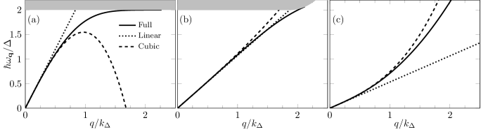
Figure 1: The RPA dispersion relation of the collective excitations is plotted (a) in the BCS regime ($1/k_{\mathrm{F}}a=-1$), (b) at unitarity ($1/k_{\mathrm{F}}|a|=0$), and (c) in the BEC regime ($1/k_{\mathrm{F}}a=1$). The full line corresponds to the full numeric solution of the dispersion, which is compared to its linear (dotted) and cubic (dashed) approximation at low $q$. The gray area shows the pair-breaking continuum. Units of the superfluid order parameter $\Delta$ and $k_{\Delta}=\sqrt{2m\Delta}/\hbar$ are used respectively for the energy and the wavenumber.

In this work we explain how dispersive waves can be used to measure the coefficient $\gamma$. Our starting point is the Schrödinger equation that governs the propagation of a plane wave of momentum $\bf{q}$:

$$\left(\mathrm{i}\partial_{t}-\omega_{\bf{q}}\right)\psi=0,$$ (2)

where $\psi\in\mathbb{R}$ represents a perturbation of the superfluid density $\rho=\rho_{0}(1+\psi)^{2}$. This very intuitive equation is in fact rigorously demonstrated for a superfluid Fermi gas by writing down, in a functional integral formalism, a quadratic Lagrangian for the phase and amplitude of the superfluid order parameter, as is done explicitly in Appendix A. Replacing $\omega_{\bf{q}}$ by its cubic approximation (1) and restricting to one dimensional right-propagating waves Eq. (2) takes the form

$$\partial_{t}\psi=-c\partial_{x}\psi+\frac{\gamma\hbar^{2}}{8m^{2}c}\partial_{x}^{3}\psi,$$ (3)

which is nothing else than a linearized Kortweg-de Vries equation Boussinesq (1877); Korteweg and de Vries (1895). The propagation of unidimensional waves in (quasi)homogeneous space can be studied in box potentials Mukherjee et al. (2017), provided the transverse size of the box is much larger than the wavelength of the perturbation Lopes et al. (2017). In elongated harmonic traps, the dispersion of phonons is expected to be concave in the BEC limit, as in a weakly interacting Bose gas Fedichev and Shlyapnikov (2001), so that no transition from subsonic to supersonic waves should occur.

We study the propagation of an initial Gaussian perturbation of the superfluid density

$$\psi(x,t=0)=\zeta\,\mathrm{e}^{-\frac{x^{2}}{2\sigma^{2}}},$$ (4)

where the amplitude $\zeta$ is chosen small enough for the linear differential equation (3) to remain valid. Upon rescaling the distances to the width of the perturbation $\sigma$ and the times to its duration $\sigma/c$, there remains a unique parameter describing the propagation of waves under Eq. (3), namely the coefficient of the third order derivative $\gamma\hbar^{2}/8m^{2}c^{2}\sigma^{2}$. This parameter thus controls the time after which the dispersive effects become important

$$t_{\mathrm{sep}}=\frac{\sigma}{|c(\tilde{q})-c|}=\frac{2\sigma}{c|\gamma|}\left(\frac{mc\sigma}{\hbar}\right)^{2}.$$ (5)

Here $c(q)=\omega_{q}/q$ is the phase velocity of the waves with momentum $q$ and $\tilde{q}=2/\sigma$ is the typical wavenumber of the high-momentum waves in the perturbation. At time $t=t_{\mathrm{sep}}$ the waves with wavenumber $\tilde{q}$ have traveled away from the main wave front across a distance $\sigma$, leading to the formation of an oscillatory train. The width $\sigma$ should be chosen small enough for the separation time to remain within experimental reach, yet large enough for the cubic expansion (1) to be valid.

In Fig. 2 we show the dispersive waves at unitarity ($1/k_{\mathrm{F}}a=0$) for $\sigma=2.5\hbar/mc$, comparing the prediction of $\gamma$ of Ref. Zou et al. (2018) to the expression of the RPA.

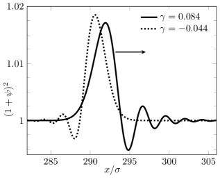
Figure 2: A comparison of dispersive waves for different predictions of the cubic coefficient $\gamma$ at unitarity ($1/k_{\mathrm{F}}a=0$). Both functions are solutions to Eq. (3), starting from a Gaussian perturbation with $\zeta=0.02$ and $\sigma=2.5\hbar/mc$. For the solid curve the analytic RPA prediction $\gamma=0.084$ is used, while the dotted line is drawn for $\gamma=-0.044$, predicted by Zou et al. Zou et al. (2018). The dispersive waves are shown at a time $t=t_{\mathrm{sep}}$ and we omitted the symmetric left-traveling wave for visibility.

The difference between supersonic and subsonic dispersive waves is clearly visible. For the positive $\gamma$ predicted by the RPA, secondary oscillations appear at the leading edge of the traveling wave, while for a negative $\gamma$ they appear at the trailing edge. Observing the location of these secondary oscillations is thus enough to predict the sign of the cubic term in the dispersion.

In the BCS regime $\gamma$ is certainly negative, offering a system with a subsonic dispersion. This can be seen in Fig. 3, where secondary oscillations appear behind the traveling wave front.

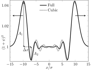
Figure 3: Dispersive waves in the BCS regime ($1/k_{\mathrm{F}}a=-1$) at a time $t=2t_{\mathrm{sep}}$, starting from an initial Gaussian perturbation with $\zeta=0.05$ and $\sigma=3.2\hbar/mc$. The cubic approximation of the dispersion (dotted line) is compared to the full numeric solution (solid line). The cubic approximation becomes worse moving away from the primary wave front, where high-momentum waves dominate.

There we compare dispersive waves generated by the full dispersion relation to those generated by its cubic approximation. Both solutions coincide close to the primary wave front, but start to differ further away, where higher wavenumbers become important and the cubic expansion is not valid anymore.

III Shock waves

To go beyond the small amplitude approximation and account for nonlinear effects in our physical situation, we now search for a nonlinear wave equation. Obtaining such an equation in a strongly interacting superfluid, and especially in a superfluid of fermions, is a difficult task. First, the (nonlinear) Korteweg-de Vries equation (or its extensions that include an arbitrary amplitude dependence of the speed of sound El et al. (2017)), which would seem like a natural generalization of Eq. (2), describes separately right- and left-travelling waves Salasnich (2011) such that it does not describe our situation where a perturbation initially at rest splits into two counter-propagating waves and where important nonlinear effects take place during the separation stage. To correctly describe counter-propagating waves, we need at least a system of two coupled nonlinear equations, as for example the (complex) Gross-Pitaevskii equation.

Second, deriving a fermionic equivalent of the Gross-Pitaevskii equation is arduous because high-amplitude excitations excite the internal degrees of freedom of the fermion pairs. A first possibility is to use Bogoliubov-de Gennes equations of motion, which are a large set of coupled nonlinear equations de Gennes (1966). Alternatively, Ref. Klimin et al. (2015) achieves it by restricting to long-wavelength and low-energy perturbations. The ensuing nonlinear wave equation on the superfluid order parameter $\Psi$ takes the following form

$$\mathrm{i}D(|\Psi|^{2})\,\partial_{t}\Psi= -C\,\partial_{x}^{2}\Psi+Q\,\partial_{t}^{2}\Psi+A(|\Psi|^{2})\Psi$$ (6)

$$+\left(E\,\partial_{x}^{2}|\Psi|^{2}-R\,\partial_{t}^{2}|\Psi|^{2}\right)\Psi,$$

where the coefficients $C$, $E$, $Q$, $R$, and the functions $A$ and $D$ of the wave intensity are given in Appendix B as integrals over the fermionic degrees of freedom. Unlike the phenomenological system based on hydrodynamics of Ref. Salasnich (2011) this equation is derived from first principles by resumming the infinite series of the slow fluctuations of the order parameter, and naturally accounts for the fermionic contribution to the wave dynamics. Unfortunately, since it truncates time and space derivatives to second order, it does not describe correctly the dispersion coefficient $\gamma$ in the BCS regime, where it depends on higher order derivatives.

In Fig. 4, we use this equation to track the time evolution of a large decrease ($\zeta=-0.3$) of the superfluid density in the BEC regime, and compare it to the linear dispersive scenario of Eq. (2). The secondary oscillations caused by the supersonic dispersion are still visible at the leading edge of the wave, but their amplitude is reduced. In the trailing edge a major nonlinear feature appears: a narrow solitary edge travelling at a constant speed. Since we chose an initial perturbation that depletes the density, this speed is here smaller than the speed of sound such that the dispersive oscillations and the solitary edge are separated by the light cone $x=\pm ct$.

The behavior observed here is reminiscent of the dispersive shock waves observed in dissipationless nonlinear media El and Hoefer (2016); Hoefer et al. (2006); Chang et al. (2008). This is remarkable since our complex nonlinear equation (6) is quite different from the Kortweg-de Vries equation with which dispersive shock waves are usually described.

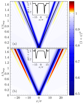
Figure 4: (Color online) The superfluid density following a localized initial perturbation in $x=0$ (with $\zeta=-0.3$ and $\sigma=1.14\hbar/mc$) is shown in colors as a function of space (on the horizontal axis) and time (on the vertical axis), in the BEC regime ($1/k_{\mathrm{F}}a=2$). The black solid lines represent the light cone $x=\pm ct$. The top panel (a) shows the nonlinear evolution according to Eq. (6) while the bottom one (b) shows the linear dispersive evolution according to Eq. (2).

IV Experimental observability

We now discuss the observability of the secondary oscillations generated by the dispersive wave propagation in real experimental conditions.

IV.1 Propagation time

To be able to see dispersive waves, one should wait a time of order $t_{\mathrm{sep}}$ (defined in Eq. (5)). At time $t=t_{\mathrm{sep}}$, no matter the value of $mc\sigma/\hbar$, the primary density excitation has an amplitude $A_{1}$ of about 95% of the initial Gaussian perturbation $\zeta$, while the biggest secondary peak $A_{2}$ is roughly 15% of $\zeta$. At this time, the spatial distance between the two peaks is approximately $\Delta x\simeq 2.6\,\sigma$.

To compare with experimental parameters, we use a system of $\mathrm{{}^{6}Li}$ atoms with a typical Fermi temperature $T_{\mathrm{F}}=1\,\mu\mathrm{K}$. Using a thin optical barrier to create the initial perturbation, one can reach a width $\sigma=1.4\,\mu\mathrm{m}$ Valtolina et al. (2017) (corresponding to $(\hbar/mc\sigma)^{2}\simeq 0.16$ at unitarity). Then the distance between the two peaks $\Delta x\simeq 3.6\,\mu\mathrm{m}$ is larger than the spatial resolution of current experiments Bloch et al. (2012); Burchianti et al. (2015). The minimal value $\gamma_{\mathrm{min}}$ that can be detected using dispersive waves is then a priori determined by the maximal propagation time in a condensate of size $L$, $t_{\mathrm{max}}=L/c$. Imposing that the maximal separation time is $t_{\mathrm{sep}}=t_{\mathrm{max}}$, taking $L=250\mu\mathrm{m}$, and $c\simeq 20\,\mu\mathrm{m/ms}$ at unitarity Joseph et al. (2007), we obtain

$$|\gamma_{\mathrm{min}}|\simeq 33\frac{\hbar}{mcL}\underset{1/k_{\mathrm{F}}|a|=0}{\simeq}0.074,$$ (7)

smaller than the value predicted by the RPA at unitarity. To illustrate, the time used in Fig. 2 is $t_{\mathrm{sep}}\simeq$20\text{\,}\mathrm{m}\mathrm{s}$$, comparable to $t_{\mathrm{max}}=$13\text{\,}\mathrm{m}\mathrm{s}$$. It should thus be possible to determine the sign of $\gamma$ at unitarity within present capabilities.

In the BCS regime $|\gamma|$ is much larger, such that shorter times are enough to distinguish dispersive waves. For an initial width $\sigma\simeq 1.2\,\mu\mathrm{m}$ ($(\hbar/mc\sigma)^{2}\simeq 0.1$), as used in Fig. 3, the separation time is $t_{\mathrm{sep}}\simeq$0.22\text{\,}\mathrm{m}\mathrm{s}$$ according to the RPA.

IV.2 Staying in the linear regime

Finally, we introduce a simple criterion on the perturbation amplitude $\zeta$ that guarantees that the waves do not enter the nonlinear regime described in Sec. III. Even if nonlinearity does not completely remove dispersive effects, it probably forbids a precise measurement of $\gamma$. We consider the nonlinear deformation of a wave packet to be significant when the propagation time exceeds Salasnich (2011)

$$t_{\mathrm{nl}}=\frac{\sigma}{|c(\zeta)-c|}.$$ (8)

Here, $c$ is the phase velocity of the low-momentum waves at density $\rho_{0}$ and $c(\zeta)$ the same velocity at density $\rho=\rho_{0}(1+\zeta)^{2}$. When $t=t_{\mathrm{nl}}$, the waves in the peak of perturbation have traveled a distance $\sigma$ away from the wave packet, therefore causing deformations of the wave front. In order for dispersive effects to be visible without nonlinear deformations, the initial perturbation $\zeta$ should be sufficiently small so that $t_{\mathrm{nl}}>t_{\mathrm{sep}}$.

Away from unitarity, where $|\gamma|$ is not anomalously small, this condition is well satisfied for perturbations of order $\zeta\approx 5\%$, for which the secondary peak $A_{2}$ has an amplitude of about 1% of the background. A density fluctuation of this magnitude is within experimental detectability Sidorenkov et al. (2013); Bloch et al. (2012). At unitarity, most theories predict $|\gamma|$ to be very small, which results in a long dispersive separation time. Therefore, fulfilling the condition $t_{\mathrm{nl}}>t_{\mathrm{sep}}$ is possible only for very small perturbations, experimentally challenging to prepare and observe. Still, the sign of $\gamma$ can be assessed by entering the nonlinear regime with more easily detectable larger perturbations. To clarify this, we extend the nonlinear wave equation (6) in order to describe a concave dispersion. The coefficient $R$ is now chosen to reproduce the desired value of $\gamma$. In Fig. 5, we use this model to compare subsonic and supersonic waves (with values of $\gamma$ as in Fig. 2) for an increase of the superfluid density ($\zeta=0.1$) sufficiently large to reveal nonlinear effects. As with more usual nonlinear dispersive wave equations El and Hoefer (2016), we observe that the orientation of the dispersive shock wave (the position of the oscillatory train with respect to the main peak) depends only on the sign of $\gamma$. This indicates that our scenario to measure the sign of $\gamma$ is robust against nonlinear effects.

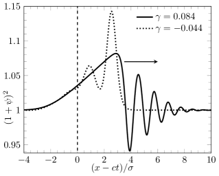
Figure 5: Wave propagation at unitarity according to Eq. (6), where the coefficients are altered to incorporate two different predictions of $\gamma$ (solid line for the RPA prediction, dotted line for the prediction of Ref. Zou et al. (2018)). Only the right-travelling wave is shown at $t=0.5t_{\mathrm{sep}}=2.8t_{\mathrm{nl}}$, from an initial perturbation with $\zeta=0.1$ and $\sigma=2.5\hbar/mc$.

V Conclusion

We have demonstrated that dispersive waves can be used as an alternative to Bragg spectroscopy Steinhauer et al. (2002); Hoinka et al. (2017) to measure the first dispersive correction to the collective branch of a superfluid Fermi gas. After a propagation time that we properly define, there appear deformations either behind or in front of the wave front, depending on whether the branch is subsonic or supersonic.

We show that using state-of-the-art experimental techniques it should be possible to assess the nature of the dispersion at unitarity. Our study takes into account possible nonlinear deformations and quantifies their relevance in experimental conditions, which is rarely done for Fermi gases.

Appendix A Equation of motion

The equation of motion (2) can be rigorously derived in the functional integral formalism. Expanding the full action of the system up to quadratic order in phase $\theta$ and amplitude $\lambda$ fluctuations of the order parameter gives the Gaussian fluctuation action Diener et al. (2008)

$$\mathcal{S}=\mathcal{S}_{0}+\int\mathrm{d}\omega\sum\limits_{\bf{q}}\begin{pmatrix}\lambda^{\ast}&\theta^{\ast}\end{pmatrix}{\bf{M}}(\omega,\bf{q})\begin{pmatrix}\lambda\\ \theta\end{pmatrix},$$ (9)

with ${\bf{M}}(\omega,\bf{q})$ the $2\times 2$ Gaussian fluctuation matrix, see Eqs. (38-39) in Ref. Kurkjian and Tempere (2017). From the action (9) coupled linear equations of motion can be derived for the phase and amplitude fields. Alternatively, one can integrate out the amplitude field $\lambda$ in the partition function

$$\mathcal{Z}=\int\,\mathcal{D}\lambda\,\mathcal{D}\theta\,\mathrm{e}^{-\mathcal{S}},$$ (10)

which yields an effective action for the phase field $\theta$

$$\tilde{\mathcal{S}}=\mathcal{S}_{0}+\int\mathrm{d}\omega\sum\limits_{\bf{q}}\frac{\det{\bf{M}}(\omega,\bf{q})}{M_{1,1}(\omega,\bf{q})}\theta^{\ast}\theta.$$ (11)

As the zeros of $\det{\bf{M}}(\omega,\bf{q})$ describe the collective mode dispersion $\omega_{\bf{q}}$, this action can always be written as

$$\tilde{\mathcal{S}}=\mathcal{S}_{0}+\int\mathrm{d}\omega\sum\limits_{\bf{q}}P(\omega,{\bf{q}})(\omega^{2}-\omega_{\bf{q}}^{2})\theta^{\ast}\theta,$$ (12)

where $P(\omega,\bf{q})$ is some polynomial in $\omega$ and $\bf{q}$ that does not vanish below the pair-breaking continuum. Extremizing the action ($\delta\mathcal{S}/\delta\theta^{\ast}=0$), switching to the time domain, and identifying $\psi$ to $\theta$ thus leads to Eq. (2) in the main text.

Appendix B Effective field theory

At zero temperature and in the 3D thermodynamic limit, the coefficients $C$, $E$, $Q$, and $R$ of Eq.(6) are given by Klimin et al. (2015)

$$C =\int\frac{\mathrm{d}\bf{k}}{(2\pi)^{3}}\frac{\hbar^{4}k^{2}}{6m^{2}}\frac{1}{4\,\mathcal{E}_{\bf{k}}^{3}}$$ (13)

$$E =\int\frac{\mathrm{d}\bf{k}}{(2\pi)^{3}}\frac{\hbar^{4}k^{2}}{3m^{2}}\frac{5\,\xi_{\bf{k}}^{2}}{16\,\mathcal{E}_{\bf{k}}^{7}}$$ (14)

$$Q =\int\frac{\mathrm{d}\bf{k}}{(2\pi)^{3}}\frac{\hbar^{2}}{8\,\mathcal{E}_{\bf{k}}^{3}}$$ (15)

$$R =\int\frac{\mathrm{d}\bf{k}}{(2\pi)^{3}}\frac{\hbar^{2}}{16\,\mathcal{E}_{\bf{k}}^{5}}$$ (16)

with $|\Delta|$ the bulk value of the superfluid order parameter and $\xi_{\bf{k}}=\frac{\hbar^{2}k^{2}}{2m}-\mu$ and $\mathcal{E}_{\bf{k}}=\sqrt{\xi_{\bf{k}}^{2}+|\Delta|^{2}}$ respectively the dispersion relations of free fermions and of BCS quasiparticles. The functions $A$ and $D$ of the perturbed order parameter $\Psi$ are

$$A(|\Psi|^{2}) =-\frac{m}{4\pi\hbar^{2}a}-\frac{1}{2}\int\frac{\mathrm{d}\bf{k}}{(2\pi)^{3}}\left(\frac{1}{E_{\bf{k}}}-\frac{2m}{\hbar^{2}k^{2}}\right)$$ (17)

$$D(|\Psi|^{2}) =\int\frac{\mathrm{d}\bf{k}}{(2\pi)^{3}}\frac{\hbar\,\xi_{\bf{k}}}{4E_{\bf{k}}^{3}}$$ (18)

with $E_{\bf{k}}=\sqrt{\xi_{\bf{k}}^{2}+|\Psi|^{2}}$.

References

- Andrews et al. (1997) M. R. Andrews, D. M. Kurn, H.-J. Miesner, D. S. Durfee, C. G. Townsend, S. Inouye, and W. Ketterle, “Propagation of sound in a Bose-Einstein condensate,” Physical Review Letters 79, 553 (1997).
- Hoinka et al. (2017) Sascha Hoinka, Paul Dyke, Marcus G. Lingham, Jami J. Kinnunen, Georg M. Bruun, and Chris J. Vale, “Goldstone mode and pair-breaking excitations in atomic Fermi superfluids,” Nature Physics 13, 943 (2017).
- Sidorenkov et al. (2013) Leonid A. Sidorenkov, Meng Khoon Tey, Rudolf Grimm, Yan-Hua Hou, Lev Pitaevskii, and Sandro Stringari, “Second sound and the superfluid fraction in a Fermi gas with resonant interactions,” Nature 498, 78 (2013).
- Delehaye et al. (2015) Marion Delehaye, Sébastien Laurent, Igor Ferrier-Barbut, Shuwei Jin, Frédéric Chevy, and Christophe Salomon, “Critical velocity and dissipation of an ultracold Bose-Fermi counterflow,” Physical Review Letters 115, 265303 (2015).
- Chevy et al. (2002) Frédéric Chevy, Vincent Bretin, Peter Rosenbusch, K. W. Madison, and Jean Dalibard, “Transverse breathing mode of an elongated Bose-Einstein condensate,” Physical Review Letters 88, 250402 (2002).
- Ozeri et al. (2002) Roee Ozeri, Jeff Steinhauer, Nadav Katz, and Nir Davidson, “Direct observation of the phonon energy in a Bose-Einstein condensate by tomographic imaging,” Physical Review Letters 88, 220401 (2002).
- Landau and Khalatnikov (1949) Lev Landau and Isaak Markovich Khalatnikov, “Teoriya vyazkosti Geliya-II,” Zh. Eksp. Teor. Fiz. 19, 637 (1949).
- Beliaev (1958) S. T. Beliaev, “Application of the methods of quantum field theory to a system of bosons,” Zh. Eksperim. i Teor. Fiz. 34, 417 (1958).
- Jochim et al. (2003) S. Jochim, M. Bartenstein, A. Altmeyer, G. Hendl, S. Riedl, C. Chin, J. Hecker-Denschlag, and R. Grimm, “Bose-Einstein Condensation of Molecules,” Science 302, 2101–2103 (2003).
- O’hara et al. (2002) K. M. O’hara, S. L. Hemmer, M. E. Gehm, S. R. Granade, and J. E. Thomas, “Observation of a strongly interacting degenerate Fermi gas of atoms,” Science 298, 2179–2182 (2002).
- Kurkjian et al. (2016a) H. Kurkjian, Yvan Castin, and A. Sinatra, “Concavity of the collective excitation branch of a Fermi gas in the BEC-BCS crossover,” Physical Review A 93, 013623 (2016a).
- Rugar and Foster (1984) D. Rugar and J. S. Foster, “Accurate measurement of low-energy phonon dispersion in liquid He 4,” Physical Review B 30, 2595 (1984).
- Lin et al. (2011) Y-J Lin, K Jimenez-Garcia, and Ian B Spielman, “Spin–orbit-coupled Bose–Einstein condensates,” Nature 471, 83 (2011).
- Kurkjian et al. (2016b) Hadrien Kurkjian, Yvan Castin, and Alice Sinatra, “Landau-Khalatnikov phonon damping in strongly interacting Fermi gases,” EPL (Europhysics Letters) 116, 40002 (2016b).
- Castin et al. (2017) Yvan Castin, Alice Sinatra, and Hadrien Kurkjian, “Landau Phonon-Roton Theory Revisited for Superfluid He 4 and Fermi Gases,” Physical Review Letters 119, 260402 (2017).
- Witham (1974) G.B. Witham, Linear and Non Linear Waves (Wiley-Interscience, 1974).
- El and Hoefer (2016) G. A. El and M. A. Hoefer, “Dispersive shock waves and modulation theory,” Physica D: Nonlinear Phenomena 333, 11–65 (2016).
- Sprenger and Hoefer (2017) Patrick Sprenger and Mark A. Hoefer, “Shock waves in dispersive hydrodynamics with nonconvex dispersion,” SIAM Journal on Applied Mathematics 77, 26–50 (2017).
- Korteweg and de Vries (1895) Diederik Johannes Korteweg and Gustav de Vries, “XLI. On the change of form of long waves advancing in a rectangular canal, and on a new type of long stationary waves,” The London, Edinburgh, and Dublin Philosophical Magazine and Journal of Science 39, 422–443 (1895).
- El et al. (2017) G. El, M. Hoefer, and M. Shearer, “Dispersive and Diffusive-Dispersive Shock Waves for Nonconvex Conservation Laws,” SIAM Review 59, 3–61 (2017).
- Klimin et al. (2015) Serghei N. Klimin, Jacques Tempere, Giovanni Lombardi, and Jozef T. Devreese, “Finite temperature effective field theory and two-band superfluidity in Fermi gases,” The European Physical Journal B 88, 122 (2015).
- Hoefer et al. (2006) M. A. Hoefer, M. J. Ablowitz, I. Coddington, Eric A. Cornell, P. Engels, and V. Schweikhard, “Dispersive and classical shock waves in Bose-Einstein condensates and gas dynamics,” Physical Review A 74, 023623 (2006).
- Chang et al. (2008) Jia J. Chang, Peter Engels, and M. A. Hoefer, “Formation of dispersive shock waves by merging and splitting Bose-Einstein condensates,” Physical Review Letters 101, 170404 (2008).
- Diener et al. (2008) Roberto B. Diener, Rajdeep Sensarma, and Mohit Randeria, “Quantum fluctuations in the superfluid state of the BCS-BEC crossover,” Physical Review A 77, 023626 (2008).
- Mañes and Valle (2009) Juan L. Mañes and Manuel A. Valle, “Effective theory for the Goldstone field in the BCS–BEC crossover at T=0,” Annals of Physics 324, 1136–1157 (2009).
- Rupak and Schäfer (2009) Gautam Rupak and Thomas Schäfer, “Density functional theory for non-relativistic fermions in the unitarity limit,” Nuclear Physics A 816, 52–64 (2009).
- Salasnich and Toigo (2008) Luca Salasnich and Flavio Toigo, “Extended Thomas-Fermi density functional for the unitary Fermi gas,” Physical Review A 78, 053626 (2008).
- Zou et al. (2018) Peng Zou, Hui Hu, and Xia-Ji Liu, “Low-momentum dynamic structure factor of a strongly interacting Fermi gas at finite temperature: The Goldstone phonon and its Landau damping,” Phys. Rev. A 98, 011602 (2018).
- Valtolina et al. (2017) G. Valtolina, F. Scazza, A. Amico, A. Burchianti, A. Recati, T. Enss, M. Inguscio, M. Zaccanti, and G. Roati, “Exploring the ferromagnetic behaviour of a repulsive Fermi gas through spin dynamics,” Nature Physics 13, 704 (2017).
- Bloch et al. (2012) Immanuel Bloch, Jean Dalibard, and Sylvain Nascimbene, “Quantum simulations with ultracold quantum gases,” Nature Physics 8, 267 (2012).
- Nascimbène et al. (2010) S. Nascimbène, N. Navon, K. J. Jiang, F. Chevy, and C. Salomon, “Exploring the thermodynamics of a universal Fermi gas,” Nature 463, 1057–1060 (2010).
- Ku et al. (2012) Mark J. H. Ku, Ariel T. Sommer, Lawrence W. Cheuk, and Martin W. Zwierlein, “Revealing the Superfluid Lambda Transition in the Universal Thermodynamics of a Unitary Fermi Gas,” Science 335, 563–567 (2012).
- Combescot et al. (2006) R. Combescot, M. Yu Kagan, and S. Stringari, “Collective mode of homogeneous superfluid Fermi gases in the BEC-BCS crossover,” Physical Review A 74, 042717 (2006).
- Boussinesq (1877) Joseph Boussinesq, Essai sur la théorie des eaux courantes (L’académie des Sciences de l’Institut National de France, 1877).
- Mukherjee et al. (2017) Biswaroop Mukherjee, Zhenjie Yan, Parth B. Patel, Zoran Hadzibabic, Tarik Yefsah, Julian Struck, and Martin W. Zwierlein, “Homogeneous Atomic Fermi Gases,” Phys. Rev. Lett. 118, 123401 (2017).
- Lopes et al. (2017) Raphael Lopes, Christoph Eigen, Adam Barker, Konrad G. H. Viebahn, Martin Robert-de Saint-Vincent, Nir Navon, Zoran Hadzibabic, and Robert P. Smith, “Quasiparticle Energy in a Strongly Interacting Homogeneous Bose-Einstein Condensate,” Phys. Rev. Lett. 118, 210401 (2017).
- Fedichev and Shlyapnikov (2001) P. O. Fedichev and G. V. Shlyapnikov, “Critical velocity in cylindrical Bose-Einstein condensates,” Phys. Rev. A 63, 045601 (2001).
- Salasnich (2011) Luca Salasnich, “Supersonic and subsonic shock waves in the unitary Fermi gas,” EPL (Europhysics Letters) 96, 40007 (2011).
- de Gennes (1966) P. G. de Gennes, Superconductivity of metals and alloys (W.A. Benjamin, New York, 1966).
- Burchianti et al. (2015) A. Burchianti, J. A. Seman, G. Valtolina, A. Morales, M. Inguscio, M. Zaccanti, and G. Roati, “All-optical production of 6Li quantum gases,” in Journal of Physics: Conference Series, Vol. 594 (IOP Publishing, 2015) p. 012042.
- Joseph et al. (2007) J. Joseph, B. Clancy, L. Luo, J. Kinast, A. Turlapov, and J. E. Thomas, “Measurement of sound velocity in a Fermi gas near a Feshbach resonance,” Physical Review Letters 98, 170401 (2007).
- Steinhauer et al. (2002) J Steinhauer, R Ozeri, N Katz, and N Davidson, “Excitation spectrum of a Bose-Einstein condensate,” Physical Review Letters 88, 120407 (2002).
- Kurkjian and Tempere (2017) Hadrien Kurkjian and Jacques Tempere, “Absorption and emission of a collective excitation by a fermionic quasiparticle in a Fermi superfluid,” New Journal of Physics 19, 113045 (2017).