Local Control Regression: Improving the Least Squares
Monte Carlo Method for Portfolio Optimization

Abstract

The least squares Monte Carlo algorithm has become popular for solving portfolio optimization problems. A simple approach is to approximate the value functions on a discrete grid of portfolio weights, then use control regression to generalize the discrete estimates. However, the classical global control regression can be expensive and inaccurate. To overcome this difficulty, we introduce a local control regression technique, combined with adaptive grids. We show that choosing a coarse grid for local regression can produce sufficiently accurate results.

Keywords: least squares Monte Carlo; local control regression; adaptive grid; control discretization; control randomization; multiperiod portfolio management

1 Introduction

The least squares Monte Carlo (LSMC) algorithm, originally introduced by [3], [15] and [18] for the pricing of American options, has become a popular tool for solving stochastic control problems in many fields, such as exotic option pricing, inventory management, project valuation, portfolio optimization and many others. The main strength of the LSMC algorithm is its ability to handle multivariate stochastic state variables, by combining the Monte Carlo simulation of the state variables with the regression estimates of the conditional expectations in the dynamic programming equations.

The purpose of this paper is to improve the control discretization approach of the LSMC algorithm for solving general portfolio optimization problems, including general investment objective functions, general intermediate costs and general asset dynamics. Before describing the details of the method, we briefly review the literature on the LSMC algorithm applied to portfolio optimization, with an emphasis on how portfolio weights are handled and how the maximization over portfolio weights is performed.

The Taylor expansion method in [1] was the first attempt to solve the portfolio optimization problems using the LSMC algorithm. The authors determine a semi-closed form solution by deriving the first-order condition of the Taylor series expansion of the investor’s future value function, see for other examples, [19], [10], and [6]. Another approach to derive and solve the first-order condition is to use [11]’s regress-later technique, see for example, [4] and [5]. However, these two first-order condition approaches, relying on analytical derivation, are restricted in the range of applications.

The simplest, most straightforward and most general approach to deal with the portfolio weights in the LSMC algorithm is to discretize them, perform one regression per discretized portfolio weight, and compute the optimal allocation for each Monte Carlo path by naive exhaustive search, see, for example, [14], [6] and [20]. Although this approach is stable and accurate, it is computationally very expensive if a fine grid is used, especially for multi-dimensional problems.

To improve the computational efficiency of the control discretization approach, control regression is a possible solution. The simplest approach is to regress state variables and portfolio weights at once. For example, in [7] and [8], the value functions are regressed on the simulated exogenous state variables, discretized wealth levels and discretized portfolio weights, and then the first-order condition is derived and solved. In [20], a control regression approach is implemented via the control randomization approach of [12]: the portfolio weights are randomized and the wealth variable is correspondingly computed in the forward simulation, afterwards the value functions are recursively regressed on the exogenous state variables, the randomized portfolio weights and wealth. However, as shown in [20], this approach may not be as accurate as the grid search approach, especially when the time horizon is long or the payoff function is highly nonlinear. Moreover, as discussed in [13], regressing on state variables and portfolio weights at once requires a very large regression, which can make it computationally difficult.

Another strand of control regression approach is introduced in [13]. The authors first regress the conditional expectations given in the first-order condition for each portfolio weight on a coarse grid, then regress the resulting regression coefficients on these portfolio weights, obtaining a hybrid generalized conditional expectation estimate expressed in both portfolio weight and state variables while keeping the size of the coarse grid of portfolio weights manageable. The regression basis of this approach is usually chosen to be polynomial (linear in [13], quadratic in [16] and [9]), in order to keep the maximization over the portfolio weights simple (constrained optimization solver in [13], analytical solution in [16] and [9]).

One such attempt is in [2]. Their approach is to sample the portfolio weights and the asset prices using low-discrepancy Sobol sequences, then use a global regression to obtain a conditional expectation estimate for every possible portfolio weight, and finally solve for the optimal portfolio weight by gradient optimization.

Building upon the aforementioned approaches, we propose a hybrid framework that adapts [20]’s combined method of control discretization and control randomization to incorporate the control regression approach of [2]. Our control regression approach differs from [2] in two main aspects, namely the use of local regression instead of global regression, and the use of adaptive refinement grids to target the region of optimal weights instead of gradient optimization. Our numerical experiments show that local control regression is more accurate and more efficient than global control regression, and that using a very coarse grid for the local control regression can produce sufficiently accurate results.

2 Problem Description

We consider a finite horizon portfolio allocation problem with one risk-free asset and $d$ risky assets available. Let $T$ be the investment horizon. We assume the portfolio can be rebalanced at any discrete time $t_{n}$ from the equally-spaced time grid $\Pi=\{t_{0}=0,t_{1},\ldots,t_{N}=T\}$. Denote by $r^{f}$ the return of the risk-free asset over a single period, by $\{\mathbf{r}_{t_{n}}\}_{0\leq n\leq N}=\{r_{t_{n}}^{i}\}_{0\leq n\leq N}^{1\leq i\leq d}$ the asset returns , by $\{\mathbf{R}_{t_{n}}\}_{0\leq n\leq N}=\{1+r_{t_{n}}^{i}\}_{0\leq n\leq N}^{1\leq i\leq d}$ the compounding factors of the asset returns, and by $\{\mathbf{S}_{t_{n}}\}_{0\leq n\leq N}=\{S_{t_{n}}^{i}\}_{0\leq n\leq N}^{1\leq i\leq d}$ the asset prices. Let $\mathbf{q}_{t_{n}}=(q_{t_{n}}^{i})_{0\leq n\leq N-1}^{1\leq i\leq d}$ describe the number of units held in each risky asset and let $\{q_{t_{n}}^{f}\}_{0\leq n\leq N-1}$ denote the amount allocated in the risk-free cash. Finally, let $\{W_{t_{n}}\}_{0\leq n\leq N}$ denote the portfolio value (wealth) process.

Let $\times$ and $\div$ denote the element-wise multiplication and division between two vectors. The asset prices evolve as

$$\mathbf{S}_{t_{n+1}}\ \ = \mathbf{S}_{t_{n}}\times\mathbf{R}_{t_{n+1}},$$ (2.1)

and the wealth process evolves as

$$W_{t_{n+1}}=W_{t_{n}}+q_{t_{n}}^{f}r^{f}+\mathbf{q}_{t_{n}}\cdot\left(\mathbf{S}_{t_{n}}\times\mathbf{r}_{t_{n+1}}\right).$$ (2.2)

Let $\mathcal{F}=\left\{\mathcal{F}_{t}\right\}_{0\leq t\leq T}$ be the filtration generated by all the state variables. At any rebalancing time $t_{n}\in\Pi$, the optimization problem is

$$v_{t_{n}}(z,w) = \sup_{\left\{\boldsymbol{\alpha}_{t_{n^{\prime}}}\in\mathcal{A}\right\}_{n\leq n^{\prime}\leq N-1}}\mbox{$\mathbb{E}$}\left[U(W_{t_{N}})\left|\mathbf{Z}_{t_{n}}=z,W_{t_{n}}=w\right.\right].$$ (2.3)

Here, $\{\mathbf{Z}_{t_{n}}\}_{0\leq n\leq N}$ is the vector of return predictors which drive the asset price dynamics $\{\mathbf{S}_{t_{n}}\}_{0\leq n\leq N}$. Thus, the variables $\{\mathbf{Z}_{t_{n}}\}_{0\leq n\leq N}$ form the exogenous state variables in our problem. The investment objective is to maximize the expected utility $\mathbb{E}[U(W_{t_{N}})]$ of the investor’s final wealth. The objective is maximized over the portfolio allocation weights in the risky assets $\boldsymbol{\alpha}_{t_{n}}=(\alpha_{t_{n}}^{i})_{0\leq n\leq N-1}^{1\leq i\leq d}$, with the allocation in the risk-free asset being equal to $\alpha_{t_{n}}^{f}=1-\sum_{1\leq i\leq d}\alpha_{t_{n}}^{i}$. The relationship between portfolio weights $\boldsymbol{\alpha}_{t_{n}}$ and portfolio positions $\mathbf{q}_{t_{n}}$ is given by $\boldsymbol{\alpha}_{t_{n}}\times W_{t_{n}}=\mathbf{S}_{t_{n}}\times\mathbf{q}_{t_{n}}$. The set $\mathcal{A}\subseteq\mathbb{R}^{d}$ of admissible strategies is assumed time-invariant for each discrete rebalancing time.

3 Least Squares Monte Carlo

In this section, we describe how to use the LSMC method to solve the dynamic portfolio optimization problem. The objective function in Eq. (2.3) can be formulated as a discrete-time dynamic programming principle,

$$v_{t_{n}}(z,w) = \sup_{\left\{\boldsymbol{\alpha}_{t_{n^{\prime}}}\in\mathcal{A}\right\}_{n\leq n^{\prime}\leq N-1}}\mbox{$\mathbb{E}$}\left[v_{t_{n+1}}\left(\mathbf{Z}_{t_{n+1}},W_{t_{n+1}}\right)\left|\mathbf{Z}_{t_{n}}=z,W_{t_{n}}=w\right.\right].$$ (3.1)

The conventional LSMC scheme simulates the state variables forward, then approximates the value functions recursively backwards in time by least squares regressions. The difficulty here stems from the conditioning wealth variable $W_{t_{n}}$, because it requires the information of all the previous portfolio decisions $\{\boldsymbol{\alpha}_{t_{n^{\prime}}}\}_{0\leq n^{\prime}\leq n}$ which are not known yet in the backward dynamic programming loop. To overcome this difficulty, a popular approach is to approximate the conditional expectations in Eq. (2.3) on a discrete grid of wealth levels, and then interpolate them on these discrete wealth levels, see for example, [1], [7] and [8].

The discretization approach can be computationally demanding if a fine grid is required, especially when there are multiple endogenous state variables. For example, when market impact is accounted for, the asset prices become endogenous state variables, which can make the discretization approach computationally infeasible.

Instead, we use a control randomization approach that simulates random portfolio weights $\{\tilde{\boldsymbol{\alpha}}_{t_{n}}^{m}\}_{0\leq n\leq N-1}^{1\leq m\leq M}$ in the forward loop in addition to the return predictors $\{\mathbf{Z}_{t_{n}}^{m}\}_{0\leq n\leq N}^{1\leq m\leq M}$, the asset returns $\{\mathbf{r}_{t_{n}}^{m}\}_{0\leq n\leq N}^{1\leq m\leq M}$, and the asset prices $\{\mathbf{S}_{t_{n}}^{m}\}_{0\leq n\leq N}^{1\leq m\leq M}$. Simulations for the wealth variable $\{\tilde{W}{}_{t_{n}}^{m}\}_{0\leq n\leq N}^{1\leq m\leq M}$ can be subsequently computed using the randomized portfolio weights. These portfolio weights are uniformly drawn from the admissible set $\mathcal{A}$, so as to ensure that the simulated sample covers the whole space of possible portfolio weights.

After all the state variables have been simulated, the next task is to approximate the conditional expectations in the dynamic programming formula in Eq. (3.1) by regression. A possible approach, called control regression, is to regress on the randomized portfolio weights as well as the return predictors, and then compute the optimal decisions by solving the first-order conditions. Such a control regression scheme, combined with control randomization, is analyzed in [12], and an application of this approach for solving dynamic portfolio optimization problem is given in [20].

However, regressing on the portfolio weights and the state variables at once requires a very large regression, which can make it computationally difficult, especially for high dimensional portfolios.

Instead, we resort to control discretization, which has been shown to be more accurate than control regression in [20]. The control space is discretized as $\mathcal{A}\approx\mathcal{A}^{\text{disc}}=\{\mathbf{a}_{1},...,\mathbf{a}_{J}\}$. At time $t_{n}$, assuming the mapping $\hat{v}_{t_{n+1}}:\left(z,w\right)\mapsto\hat{v}_{t_{n+1}}\left(z,w\right)$ has been estimated, the dynamic programming principle in Eq. (3.1) becomes

$$v_{t_{n}}(z,w)=\max_{\mathbf{a}_{j}\in\mathcal{A}^{\text{disc}}}\mathbb{E}\left[\hat{v}_{t_{n+1}}\left(\mathbf{Z}_{t_{n+1}},W_{t_{n+1}}\right)\left|\mathbf{Z}_{t_{n}}=z,W_{t_{n}}=w,\boldsymbol{\alpha}_{t_{n}}=\mathbf{a}_{j}\right.\right]=:\max_{\mathbf{a}_{j}\in\mathcal{A}^{\text{disc}}}\text{CV}_{t_{n}}^{j}\left(z,w\right),$$

where $\text{CV}_{t_{n}}^{j}$ denotes the continuation value function of choosing the portfolio weight $\mathbf{a}_{j}$ at time $t_{n}$. To evaluate $\text{CV}_{t_{n}}^{j}$ for each $\mathbf{a}_{j}\in\mathcal{A}^{\text{disc}}$, we first update the portfolio weights $\boldsymbol{\alpha}_{t_{n}}^{m}=\mathbf{a}_{j}$ for each Monte Carlo path $m=1,...,M$. Then, the wealth variables at time $t_{n+1}$ can be recomputed based on the portfolio weight $\mathbf{a}_{j}$,

$$\mathbf{q}_{t_{n}}^{m,j} = \mathbf{a}_{j}\times\tilde{W}_{t_{n}}^{m}\div\mathbf{S}_{t_{n}}^{m}$$

$$\hat{W}_{t_{n+1}}^{m,(n,j)} = \tilde{W}_{t_{n}}^{m}+q_{t_{n}}^{f,m,j}r^{f}+\mathbf{q}_{t_{n}}^{m,j}\cdot\left(\mathbf{S}_{t_{n}}^{m}\times\mathbf{r}_{t_{n+1}}^{m}\right),$$

where $\hat{W}_{t_{n+1}}^{m,(n,j)}$ is the recomputed wealth at time $t_{n+1}$ conditioning on the information at time $t_{n}$ at the $j^{\text{th}}$ node of the control grid. Let $\{\psi_{k}\left(z,w\right)\}_{1\leq k\leq K}$ be the basis functions of the state variables for the regression. For each portfolio decision $\mathbf{a}_{j}\in\mathcal{A}^{\text{disc}}$, the corresponding $\text{CV}_{t_{n}}^{j}$ is approximated by least squares minimization:

$$\left\{\hat{\beta}_{k,t_{n}}^{j}\right\}_{1\leq k\leq K} = \arg\min_{\left\{\beta_{k}\right\}_{1\leq k\leq K}}\sum_{m=1}^{M}\left(\hat{v}_{t_{n+1}}\left(\mathbf{Z}_{t_{n+1}}^{m},\hat{W}_{t_{n+1}}^{m,(n,j)}\right)-\sum_{k=1}^{K}\beta_{k}\psi_{k}\left(\mathbf{Z}_{t_{n}}^{m},\tilde{W}{}_{t_{n}}^{m}\right)\right)^{2}.$$

Finally, $\text{CV}_{t_{n}}^{j}$ is parametrized as

$$\hat{\text{CV}}_{t_{n}}^{j}\left(z,w\right) = \sum_{k=1}^{K}\beta_{k,t_{n}}^{j}\psi_{k}\left(z,w\right),$$

and the optimal decision policy is

$$\hat{\boldsymbol{\alpha}}_{t_{n}}\left(z,w\right)=\arg\max_{\mathbf{a}_{j}\in\mathcal{A}^{\text{disc}}}\hat{\text{CV}}_{t_{n}}^{j}\left(z,w\right), \hat{v}\left(z,w\right)=\max_{\mathbf{a}_{j}\in\mathcal{A}^{\text{disc}}}\hat{\text{CV}}_{t_{n}}^{j}\left(z,w\right),$$

where the maximization is performed by an exhaustive grid search.

As tested in [20], the control discretization approach is numerically very stable, even when transaction costs and price impact are taken into account. However, the exhaustive grid search is computationally very expensive, especially for high dimensional portfolios. In the next section, we will introduce a local control regression method to reduce the computational burden of control discretization.

4 Control Regression and Maximization

After the value functions have been estimated on the discrete grid $\mathcal{A}^{\text{disc}}$, the next step is to use control regression to project these discrete estimates onto a continuous space of control. This section describes in detail how to use control regression to improve the estimates. For notional convenience, we denote by $\hat{\text{CV}}^{j}=\hat{\text{CV}}^{j}\left(z,w\right)$ the estimated continuation value of choosing the portfolio weight $\mathbf{a}_{j}$ at an arbitrary time and for an arbitrary input of state variables $(z,w)$. Suppose we have already implemented the grid search approach to estimate the conditional values $\hat{\text{CV}}^{j}$ on a coarse discrete grid $\mathcal{A}^{\text{disc}}$, and have estimated the optimal control by the following equation

$$\hat{\boldsymbol{\alpha}}=\arg\max_{\mathbf{a}_{j}\in\mathcal{A}^{\text{disc}}}\hat{\text{CV}}^{j}.$$ (4.1)

The usual approach to generalize these conditional value estimates on the discrete grid $\mathcal{A}^{\text{disc}}$ is to use global regression, see for example [13] and [2]. However, it can be hard to find a regression basis that fits the global grid well, even when using advanced regression techniques. As an example, Figure 4.1 illustrates the global regression approach for a portfolio with risk-free cash and two risky assets ($d=2$). Moreover, even if adequate regression basis can be found, the global regression can be computationally very expensive. In fact, it is unnecessary to project the discrete value functions onto the whole global control space, because what matters for maximizing the value functions is the accuracy on the small local region containing the optimum.

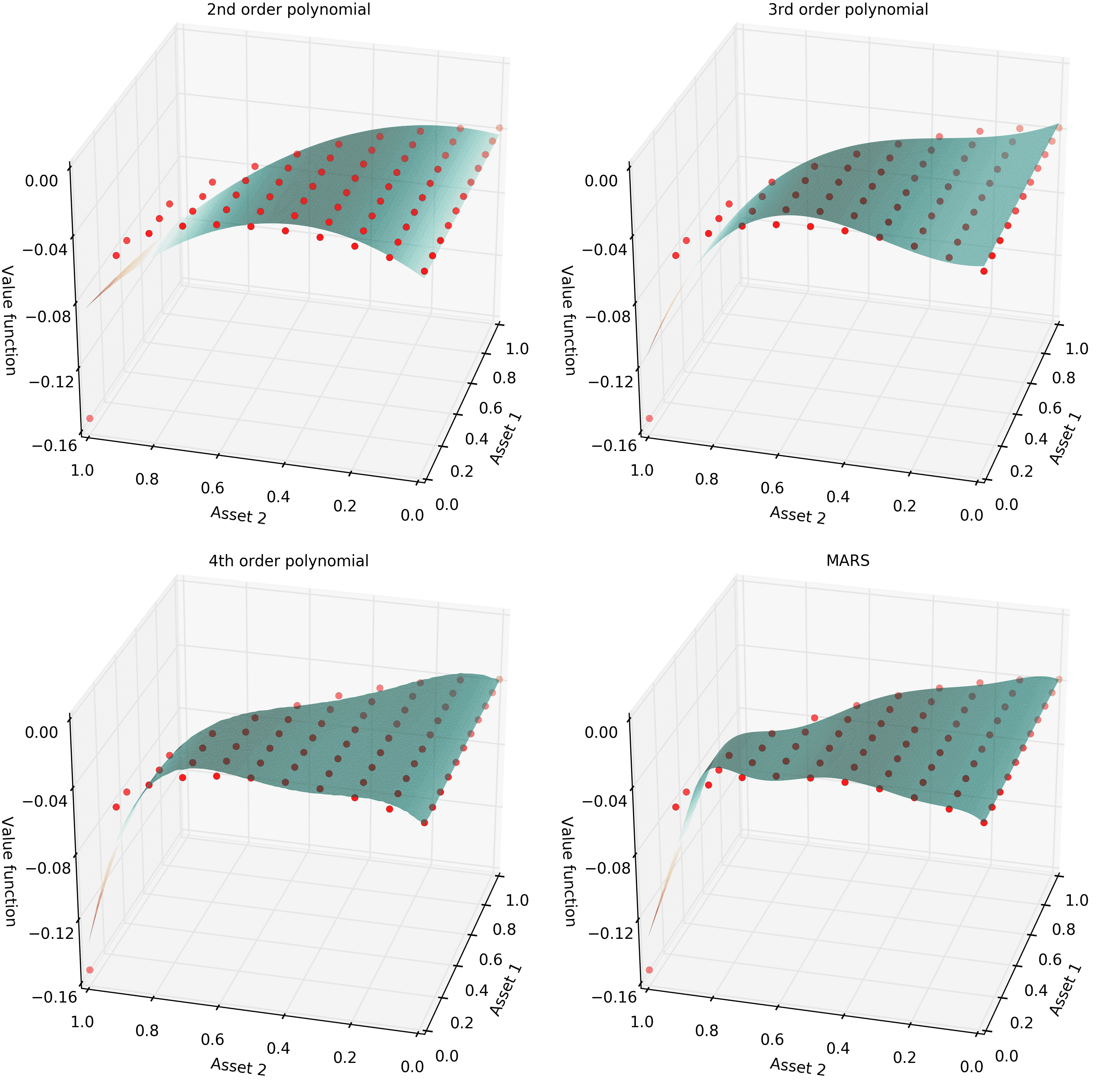
Figure 4.1: Global control regression

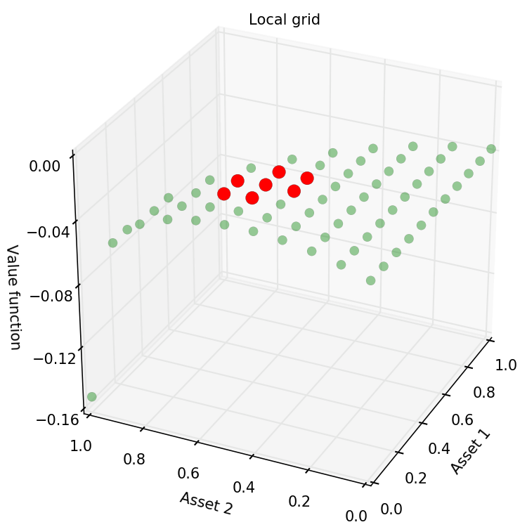
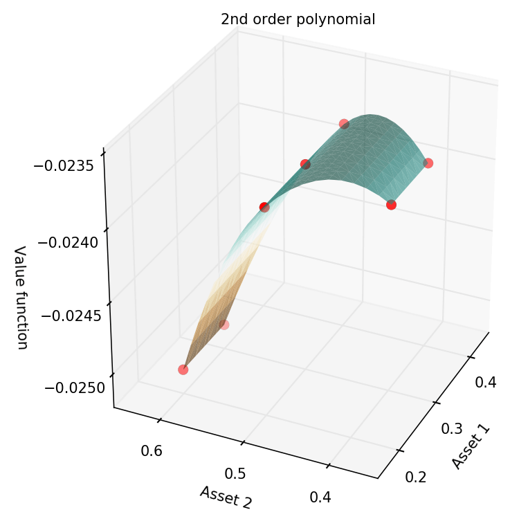
Figure 4.2: Local control regression

The left panel highlights the local control grid (in red) out of the global grid (in green) and the right panel shows the fitted surface on the selected local grid.

4.1 Local control regression

In order to improve the numerical accuracy and efficiency of control regression, we propose to perform a local regression around the optimal estimate $\hat{\boldsymbol{\alpha}}$. We construct a local grid $\mathcal{L}^{\text{disc}}(\hat{\boldsymbol{\alpha}})\subset\mathcal{A}^{\text{disc}}$ that contains the neighbors of $\hat{\boldsymbol{\alpha}}$ :

$$\mathcal{L}^{\text{disc}}\left(\hat{\boldsymbol{\alpha}}\right):=\left\{\mathbf{a}\in\mathcal{A}^{\text{disc}}:\left\|\hat{\boldsymbol{\alpha}}-\mathbf{a}\right\|_{\infty}\leq\delta\right\},$$ (4.2)

where $\delta$ is the mesh size of the discrete grid $\mathcal{A}^{\text{disc}}$. Then, we regress the estimated conditional values $\hat{\text{CV}}^{j}$ with respect to the points in the local grid $\mathcal{L}^{\text{disc}}(\hat{\boldsymbol{\alpha}})$, obtaining the parametric conditional value estimates $\hat{\Phi}\left(\mathbf{a}\right)$ over the whole continuous local control hypercube

$$\mathcal{L}^{\text{cont}}\left(\hat{\boldsymbol{\alpha}}\right):=\left\{\mathbf{a}\in\mathcal{A}:\left\|\hat{\boldsymbol{\alpha}}-\mathbf{a}\right\|_{\infty}\leq\delta\right\}.$$ (4.3)

The main advantage of local regression is a better goodness-of-fit, as the local grid $\mathcal{L}^{\text{disc}}\left(\hat{\boldsymbol{\alpha}}\right)$ contains only very few points and are therefore easier to fit even with simple bases such as local second-order polynomial bases. In addition, a simple second-order polynomial is a sensible candidate for such a local parametric regression, as the local grid only contains a maximum of three points in each dimension and the maximum lies at either the middle point or the boundary of the local coarse grid. Furthermore, to guarantee the robustness of local regression, we perform local Ridge regressions with second-order polynomial bases. Figure 4.2 illustrates the local control regression approach on the same example presented in Figure 4.1.

Now that continuation value estimates have been obtained over the whole local hypercube $\mathcal{L}^{\text{cont}}(\hat{\boldsymbol{\alpha}})$, we turn to the problem of estimating the optimal control over $\mathcal{L}^{\text{cont}}(\hat{\boldsymbol{\alpha}})$, i.e.,

$$\hat{\boldsymbol{\alpha}}^{*} = \arg\max_{\mathbf{a}\in\mathcal{L}^{\text{cont}}\left(\hat{\boldsymbol{\alpha}}\right)}\hat{\Phi}\left(\boldsymbol{a}\right).$$ (4.4)

4.2 Maximization by adaptive grids

The next step is to improve the discrete optimal control estimate in Eq. (4.1) by solving the continuous equation in Eq. (4.4). Classical approaches to do so are to use gradient optimization which requires either analytically or numerically compute the gradients. Instead, we perform the maximization using a gradient-free adaptive refinement strategy.

Here is a simple illustration of this adaptive grid method. Suppose we are given a portfolio of a risk-free asset and a risky asset. We denote by $\{\mathcal{A}_{p}\}_{0\leq p\leq P}$ the sequence of adaptive grids and denote by $\{\delta_{p}\}_{0\leq p\leq P}$ the sequence as adaptive mesh sizes such that $\delta_{p+1}=\delta_{p}/2$. We define the initial adaptive grid as $\mathcal{A}_{0}=\mathcal{A}^{\text{disc}}$ and define the initial control mesh size as $\delta_{0}=\delta$. Suppose the optimal control $\hat{\alpha}_{0}$ has been estimated on the space $\mathcal{A}_{0}=\mathcal{A}^{\text{disc}}$. Then, the updated adaptive grid is defined as $\mathcal{A}_{1}=\{\hat{\alpha}_{0}-\delta_{0}/2,\hat{\alpha}_{0},\hat{\alpha}_{0}+\delta_{0}/2\}$ and the updated estimate of optimal control is given by $\hat{\alpha}_{1}=\arg\max_{a\in\mathcal{A}_{1}}\hat{\Phi}\left(a\right)$. Iteratively, the adaptive grid will be $\mathcal{A}_{p}=\{\hat{\alpha}_{p-1}-\delta/2^{p},\hat{\alpha}_{p-/1},\hat{\alpha}_{p-1}+\delta/2^{p}\}$. For every refined adaptive grid, there is a maximum of two new points in each dimension of the control. This hierarchical structure guarantees a limited number of operations will be performed in the algorithm. Below is an example of our adaptive grid refinement strategy starting with a $\delta=1/4$ control mesh for $\mathcal{A}^{\text{disc}}$:

$$\mathcal{A}^{\text{d}}= \mathcal{A}_{0}=\{0,\,0.2500,\,0.5000,\,0.7500,\,1\}$$

$$\text{\text{Suppose }}\hat{\alpha}_{0}=\arg\max_{a\in\mathcal{A}_{0}}\hat{\Phi}\left(a\right)=0.5000, \mathcal{A}_{1}=\{0.3750,\,0.5000,\,0.6250\}$$ then

$$\text{Suppose }\hat{\alpha}_{1}=\arg\max_{a\in\mathcal{A}_{1}}\hat{\Phi}\left(a\right)=0.3750, \mathcal{A}_{2}=\{0.3125,\,0.3750,\,0.4375\}$$ then

$$\text{Suppose }\hat{\alpha}_{2}=\arg\max_{a\in\mathcal{A}_{2}}\hat{\Phi}\left(a\right)=0.3125, \mathcal{A}_{3}=\{0.28125,\,0.3125,\,0.34375\}$$ then

$$\text{Suppose }\hat{\alpha}_{3}=\arg\max_{a\in\mathcal{A}_{3}}\hat{\Phi}\left(a\right)=0.3125, \mathcal{A}_{4}=\{0.296875,\,0.3125,\,0.32815\}$$ then

$$\vdots$$

$$\text{Finally }\hat{\alpha}^{*}:=\arg\max_{a\in\mathcal{A}_{P}}\hat{\Phi}\left(a\right)$$

One can see that it takes only five iterations to reach a control mesh precision higher than $1/100$, and only a maximum of two extra evaluation points are required at each iteration. This adaptive grid method can be described as a modified multivariate bisection search for the local maximum of a function. The combination of local regression and adaptive grids is described in Algorithm 1. In our experience, both gradient optimization and adaptive grids can reach the optimum but the latter is more efficient.

1:  Input: $\left\{\hat{\text{CV}}^{j}\right\}_{1\leq j\leq J}$

2:  Result: $\hat{\boldsymbol{\alpha}}^{*}$

3:  Find the optimal decision on the coarse grid by grid searching:

$$\hat{\boldsymbol{\alpha}}_{0}=\arg\max_{\mathbf{a}_{j}\in\mathcal{A}^{\text{disc}}}\hat{\text{CV}}{}^{j}$$

4:  Construct a local grid in the neighbourhood of $\hat{\boldsymbol{\alpha}}$:

$$\mathcal{L}^{\text{disc}}\left(\hat{\boldsymbol{\alpha}}_{0}\right):=\left\{\mathbf{a}\in\mathcal{A}^{\text{disc}}:\left\|\hat{\boldsymbol{\alpha}}_{0}-\mathbf{a}\right\|_{\infty}\leq\delta\right\}$$

5:  Regress $\left\{\hat{\text{CV}}^{j}\right\}_{\mathbf{a}_{j}\in\mathcal{L}^{\text{disc}}\left(\hat{\boldsymbol{\alpha}}_{0}\right)}$ on $\mathcal{L}^{\text{disc}}\left(\hat{\boldsymbol{\alpha}}_{0}\right)$, obtaining a parametric shape $\hat{\Phi}\left(\boldsymbol{\alpha}_{0}\right)$ on

$$\mathcal{L}^{\text{cont}}\left(\hat{\boldsymbol{\alpha}}_{0}\right):=\left\{\mathbf{a}\in\mathcal{A}:\left\|\hat{\boldsymbol{\alpha}}_{0}-\mathbf{a}\right\|_{\infty}\leq\delta\right\}.$$

6:  Set the initial adaptive grid $\mathcal{A}_{0}=\mathcal{L}^{\text{disc}}\left(\hat{\boldsymbol{\alpha}}_{0}\right)$

7:  for each $p=1,\ldots,P$ do

8:     Update adaptive grid: $\mathcal{A}_{p}:=\left\{\mathbf{a}\in\mathcal{L}^{\text{cont}}\left(\hat{\boldsymbol{\alpha}}_{0}\right):\mathbf{a}=\hat{\boldsymbol{\alpha}}_{p-1}\pm\delta/2^{p}\right\}\cup\left\{\hat{\boldsymbol{\alpha}}_{p-1}\right\}$

9:     Update adaptive control estimate: $\hat{\boldsymbol{\alpha}}_{p}=\arg{\displaystyle\max_{\mathbf{a}\in\mathcal{A}_{p}}}\hat{\Phi}\left(\mathbf{a}\right)$

10:  end for

11:  $\hat{\boldsymbol{\alpha}}^{*}:=\hat{\boldsymbol{\alpha}}_{P}$

Algorithm 1 Local regression and adaptive grids

5 Numerical Experiments

In this section, we validate the numerical method proposed in the previous sections by applying it to a multiperiod portfolio optimization problem as formulated in Section 2.

We obtain monthly close prices from October 2007 to January 2016 of 13 financial assets (ETF tickers: BND, SPY, EFA, EEM, GLD, BWX, SLV, USO, UUP, FXE, FXY, and FXA) from Yahoo finance. We calibrate a first-order vector autoregressive model to log-returns ($\log S_{t}-\log S_{t-1}$) to obtain the return dynamics. We fix the annual interest rate on the cash account to $4.5\%$. We consider a three-dimensional portfolio optimization with the cash component, BND and SPY. The rest of the 11 financial assets are used as exogenous return predictors for BND and SPY. In the numerical tests, we use a sample of $M=10^{4}$ Monte Carlo paths.

We assume transaction costs of $0.3\%$ proportional to the portfolio turnover. For liquidity costs and market impact which depend on the transaction volume, we describe the price movement during the transaction by the marginal supply-demand curve (MSDC) calibrated by [17] to the European medium- and large-cap equities. The MSDC reads

$$\textrm{MSDC}\left(\Delta q\right)=\begin{cases}S_{\text{A}}e^{k\sqrt{\left|\Delta q\right|}}&\mathrm{when}\,q>0\,\text{(position increase)}\\ S_{\text{B}}e^{-k\sqrt{\left|\Delta q\right|}}&\mathrm{when}\,q<0\,\mbox{\text{(position reduction})}\end{cases},$$ (5.1)

where $S_{\mathrm{B}}$ denotes the best bid price, $S_{\mathrm{A}}$ denotes the best ask price, $\Delta q$ denotes the position change of the investor at time $t$ and $k\in\mathbb{R}^{+}$ is called the liquidity risk factor. By integrating with respect to $\Delta q$ , we obtain an explicit parametric form for the liquidity costs,

$$\textrm{LC}\left(\Delta q\right)=S_{\text{A}}\left(\lambda\left(\Delta q\right)-\Delta q\right)\mathbbm{1}\left\{\Delta q>0\right\}+S_{\text{B}}\left(q-\lambda\left(\Delta q\right)\right)\mathbbm{1}\left\{\Delta q<0\right\}\,,$$

where $\lambda(\Delta q)=\frac{2}{k^{2}}(\mathrm{sign}(\Delta q)k\sqrt{|\Delta q|}e^{-\mathrm{sign}(q)k\sqrt{|\Delta q|}}+e^{-\mathrm{sign}(\Delta q)k\sqrt{|\Delta q|}}-1).$ Following the calibration results from [17], we set $k=8\times 10^{-6}$. The calibrated bid-ask spread $S_{\text{A}}-S_{\text{B}}$ is about $10^{-5}$, which, according to our tests, is small enough to have virtually no impact on the optimal portfolio allocation. For convenience, we simply set $S_{\text{B}}=S_{\text{A}}$. The permanent market impact can be deemed proportional to the temporary peak of the MSDC. We assume $2/3$ for the proportional rate for the market impact. For the details of how to incorporate these switching costs into the LSMC method, we refer to [20].

We use the constant relative risk aversion (CRRA) utility, i.e., $U(w)=w^{1-\gamma}/(1-\gamma)$. for the optimization objective. We report our numerical results in terms of monthly adjusted certainty equivalent returns (CER) given by $\mathrm{CER}=U^{-1}(\mathbb{E}[U(W_{T})])^{\frac{1}{T}}-1\approx U^{-1}(\frac{1}{M}\sum_{m=1}^{M}U(W_{T}^{m}))^{\frac{1}{T}}-1.$ The magnitude of monthly returns is usually less than one percent, thus we report CER in basis points to make comparisons easier.

5.1 Local regression v.s. global regression

As explained in Section 4.1, the optimal portfolio allocation computed on a discrete grid can be improved by control regression. Here, we compare local control regression and global control regression in terms of accuracy and efficiency, given that both use adaptive grids to find the optimum. Table 5.1 and Table 5.2 compare local regression to different types of global bases. Our results show that local regression does improve both accuracy and efficiency. The outlier value $-12.3$ in Table 5.1 for $4^{\text{th}}$-order global polynomial regression and $\delta=1/8$ suggests that high-order polynomial bases may produce unreliable results.

Table 5.1: CER for different regression methods and different mesh sizes

		$2^{\text{nd}}$ Local		$2^{\text{nd}}$ Global		$3^{\text{rd}}$ Global		$4^{\text{th}}$ Global		MARS Global
$\delta=1/2$		$64.9$		$65.0$		$64.9$		$64.8$		$63.2$
$\delta=1/4$		$65.0$		$64.8$		$65.0$		$64.9$		$64.5$
$\delta=1/8$		$65.1$		$64.9$		$64.5$		$-12.3$		$65.0$
$\delta=1/16$		$65.2$		$64.8$		$64.9$		$65.0$		$65.0$
$\delta=1/32$		$65.2$		$64.8$		$64.7$		$65.0$		$64.8$

This table compares the lower bound of the truncated VFI scheme for the monthly adjusted CER (in basis points) using different sizes of control mesh and different regression bases. A CRRA investment style with $\gamma=10$ over a 6-month horizon ($N=6$ months) is considered.

Table 5.2: Computational runtime for different regression methods and different mesh sizes

		$2^{\text{nd}}$ Local		$2^{\text{nd}}$ Global		$3^{\text{rd}}$ Global		$4^{\text{th}}$ Global		MARS Global
$\delta=1/2$		$\tau^{a}=43$ secs		$1.2\times\tau^{a}$		$1.6\times\tau^{a}$		$2.6\times\tau^{a}$		$3.6\times\tau^{a}$
$\delta=1/4$		$\tau^{b}=1.5$ mins		$1.4\times\tau^{b}$		$1.9\times\tau^{b}$		$3.0\times\tau^{b}$		$10.5\times\tau^{b}$
$\delta=1/8$		$\tau^{c}=5.2$ mins		$1.8\times\tau^{c}$		$2.3\times\tau^{c}$		$7.0\times\tau^{c}$		$15.6\times\tau^{c}$
$\delta=1/16$		$\tau^{d}=24.1$ mins		$2.8\times\tau^{d}$		$3.9\times\tau^{d}$		$9.3\times\tau^{d}$		$22.3\times\tau^{d}$
$\delta=1/32$		$\tau^{e}=2.9$ hours		$4.1\times\tau^{e}$		$7.0\times\tau^{e}$		$13.6\times\tau^{e}$		$35.4\times\tau^{e}$

This table reports the computational runtime w.r.t. control dimension of approximating conditional expectations for one time step under different sizes of mesh and different regression bases. A CRRA investment style with $\gamma=10$ over a 6-month horizon ($N=6$ months) is considered. For ease of comparison, the results are reported as multiple of the fastest method (local regression).

5.2 Mesh size

We then test the sensitivity of the accuracy (Table 5.3) and efficiency (Table 5.4) with respect to the mesh size of the control grid. Table 5.3 shows that a coarse grid ($\delta=1/8$) combined with local control regression is able to produce accurate results: the errors in CER and initial portfolio allocation are negligible compared to a fine grid ($\delta=1/32$).

Table 5.4 reports the runtime of one time step iteration of the backward dynamic programming for different control meshes. The main message coming from these results is that although we still do not completely get rid of the curse of dimensionality, the presented technique allows us to solve portfolio optimization problems of much greater size (more than ten risky assets) than what is usually considered in the literature (less than three risky assets).

It is important to note that, in order to properly compare the runtime, the code is written based on naive “for loop” for each Monte Carlo path and the computational speed can be greatly improved by vectorization or by using lower level programming languages. In particular, the code is implemented in Python 3.4.3 on a single processor Intel Core i7 2.2 GHz.

Table 5.3: CER and initial optimal allocation with different mesh sizes

				CER				Initial weights $\boldsymbol{\alpha}$
				$\gamma\!=\!5$	$\gamma\!=\!10$	$\gamma\!=\!15$		$\gamma\!=\!5$	$\gamma\!=\!10$	$\gamma\!=\!15$
$N=3$		$\delta=1/2$		$66.6$	$57.5$	$47.3$		$0.51$, $0.37$, $0.12$	$0.78$, $0.22$, $0.00$	$1.00$, $0.00$, $0.00$
		$\delta=1/4$		$66.6$	$57.6$	$47.8$		$0.41$, $0.31$, $0.18$	$0.65$, $0.22$, $0.13$	$0.95$, $0.05$, $0.00$
		$\delta=1/8$		$66.4$	$57.8$	$48.0$		$0.42$, $0.32$, $0.16$	$0.64$, $0.23$, $0.13$	$0.92$, $0.08$, $0.00$
		$\delta=1/16$		$66.6$	$57.8$	$47.8$		$0.42$, $0.33$, $0.15$	$0.65$, $0.24$, $0.11$	$0.92$, $0.08$, $0.00$
		$\delta=1/32$		$66.7$	$57.8$	$48.0$		$0.41$, $0.32$, $0.17$	$0.64$, $0.26$, $0.10$	$0.92$, $0.08$, $0.00$
$N=6$		$\delta=1/2$		$80.8$	$64.9$	$49.7$		$0.65$, $0.27$, $0.08$	$0.85$, $0.15$, $0.00$	$1.00$, $0.00$, $0.00$
		$\delta=1/4$		$80.8$	$65.0$	$50.2$		$0.58$, $0.31$, $0.11$	$0.77$, $0.18$, $0.05$	$1.00$, $0.00$, $0.00$
		$\delta=1/8$		$80.6$	$65.1$	$50.5$		$0.57$, $0.31$, $0.12$	$0.75$, $0.20$, $0.05$	$0.91$, $0.09$, $0.00$
		$\delta=1/16$		$80.7$	$65.2$	$50.5$		$0.55$, $0.32$, $0.13$	$0.74$, $0.20$, $0.06$	$0.92$, $0.08$, $0.00$
		$\delta=1/32$		$80.8$	$65.2$	$50.5$		$0.55$, $0.32$, $0.13$	$0.71$, $0.22$, $0.07$	$0.92$, $0.08$, $0.00$
$N=12$		$\delta=1/2$		$86.5$	$66.7$	$51.0$		$0.87$, $0.13$, $0.00$	$1.00$, $0.00$, $0.00$	$1.00$, $0.00$, $0.00$
		$\delta=1/4$		$86.7$	$67.1$	$51.0$		$0.81$, $0.19$, $0.00$	$0.90$, $0.10$, $0.00$	$0.86$, $0.14$, $0.00$
		$\delta=1/8$		$86.5$	$67.2$	$51.2$		$0.82$, $0.18$, $0.00$	$0.89$, $0.11$, $0.00$	$0.88$, $0.12$, $0.00$
		$\delta=1/16$		$86.6$	$67.4$	$51.1$		$0.81$, $0.19$, $0.00$	$0.87$, $0.13$, $0.00$	$0.88$, $0.12$, $0.00$
		$\delta=1/32$		$86.8$	$67.4$	$51.1$		$0.81$, $0.19$, $0.00$	$0.87$, $0.13$, $0.00$	$0.88$, $0.12$, $0.00$

This table compares the monthly adjusted CER (in basis points) and the initial optimal portfolio allocation using different sizes of control mesh ($\delta=1/2,1/4,1/8,1/16,1/32$) under different investment horizons ($N=3,6,12$ months) and different risk-aversion parameters of the CRRA utility ($\gamma=5,10,15$).

Table 5.4: Computational runtime with different control dimensions

		$\delta=1/2$		$\delta=1/4$		$\delta=1/8$		$\delta=1/16$		$\delta=1/32$
$d=2$		$19\text{ secs}$		$26\text{ secs}$		$48\text{ secs}$		$1.6\text{ mins}$		$3.2\text{ mins}$
$d=3$		$43\text{ secs}$		$1.5\text{ mins}$		$5.2\text{ mins}$		$24.1\text{ mins}$		$2.9\text{ hrs}$
$d=4$		$1.4\text{ mins}$		$4.5\text{ mins}$		$29.4\text{ mins}$		$8.6\text{ hrs}$		N\A
$d=5$		$2.4\text{ mins}$		$11.8\text{ mins}$		$2.9\text{ hrs}$		N\A		N\A
$d=6$		$3.9\text{ mins}$		$37.2\text{ mins}$		$13.8\text{ hrs}$		N\A		N\A
$d=7$		$6.1\text{ mins}$		$1.3\text{ hrs}$		N\A		N\A		N\A
$d=8$		$9.1\text{ mins}$		$2.2\text{ hrs}$		N\A		N\A		N\A
$d=9$		$14.0\text{ mins}$		$3.5\text{ hrs}$		N\A		N\A		N\A
$d=10$		$19.6\text{ mins}$		$6.4\text{ hrs}$		N\A		N\A		N\A

This table reports the computational runtime w.r.t. control dimension of performing one time step conditional expectation approximation under different sizes of mesh ($\delta=1/2,1/4,1/8,1/16,1/32$). “N\A” indicates the situation where the program takes more than 24 hours to run.

6 Conclusion

This paper designs an improved LSMC method for solving stochastic control problems. This LSMC modification can be summarized as follows: we first estimate the value functions on a discrete grid of controls, then generalize the discrete estimates by local control regression, and finally determine the optimal (continuous) control by an adaptive refinement algorithm. We apply the method to a dynamic multivariate portfolio optimization problem in the presence of transaction costs, liquidity costs and market impact. We numerically show that the local regression of continuation estimates with respect to portfolio weights is more accurate and more efficient than the classical global control regression. We show that the combination of local control regression and adaptive grids significantly improves the computational efficiency without sacrificing accuracy, and that accurate results can be obtained from very coarse grids.

References

- Brandt et al. [2005] Brandt, M., A. Goyal, P. Santa-Clara, and J. Stroud (2005). A simulation approach to dynamic portfolio choice with an application to learning about return predictability. Review of Financial Studies 18(3).
- Broadie and Shen [2016] Broadie, M. and W. Shen (2016). High-dimensional portfolio optimization with transaction costs. International Journal of Theoretical and Applied Finance 19(4), 1650025.
- Carriere [1996] Carriere, J. (1996). Valuation of the early-exercise price for options using simulations and nonparametric regression. Insurance: Mathematics and Economics 19(1), 19–30.
- Cong and Oosterlee [2016a] Cong, F. and C. W. Oosterlee (2016a). Multi-period mean-variance portfolio optimization based on Monte Carlo simulation. Journal of Economic Dynamics and Control 64(1), 23–38.
- Cong and Oosterlee [2016b] Cong, F. and C. W. Oosterlee (2016b). On pre-commitment aspects of a time-consistent strategy for a mean-variance investor. Journal of Economic Dynamics and Control 70(1), 178–193.
- Cong and Oosterlee [2017] Cong, F. and C. W. Oosterlee (2017). Accurate and robust numerical methods for the dynamic portfolio management problem. Computational Economics 49(3), 433–458.
- Denault et al. [2017] Denault, M., E. Delage, and J.-G. Simonato (2017). Dynamic portfolio choice: a simulation-and-regression approach. Optimization and Engineering 18(2), 369–406.
- Denault and Simonato [2017] Denault, M. and J.-G. Simonato (2017). Dynamic portfolio choices by simulation-and-regression: Revisiting the issue of value function vs portfolio weight recursions. Computers and Operations Reseach 79, 174–189.
- Diris et al. [2015] Diris, B., F. Palm, and P. Schotman (2015). Long-term strategic asset allocation: an out-of-sample evaluation. Management Science 61(9), 2185–2202.
- Garlappi and Skoulakis [2010] Garlappi, L. and G. Skoulakis (2010). Solving consumption and portfolio choice problems: The state variable decomposition method. Review of Financial Studies 23, 3346–3400.
- Glasserman and Yu [2002] Glasserman, P. and B. Yu (2002). Simulation for American options: Regression now or regression later? Monte Carlo and Quasi-Monte Carlo Methods 2002, 213–226.
- Kharroubi et al. [2014] Kharroubi, I., N. Langrené, and H. Pham (2014). A numerical algorithm for fully nonlinear HJB equations: an approach by control randomization. Monte Carlo Methods and Applications 20(2), 145–165.
- Koijen et al. [2010] Koijen, R., T. Nijman, and B. Werker (2010). When can life cycle investors benefit from time-varying bond risk premia. The Review of Financial Studies 23(2), 741–780.
- Koijen et al. [2009] Koijen, R., J. C. Rodríguez, and A. Sbuelz (2009). Momentum and mean reversion in strategic asset allocation. Management Science 55(7), 1199–1213.
- Longstaff and Schwartz [2001] Longstaff, F. and E. Schwartz (2001). Valuing American options by simulation: A simple least-squares approach. Review of Financial Studies 14(1), 681–692.
- Shen et al. [2014] Shen, S., A. Pelsser, and P. Schotman (2014). Robust long-term interest rate risk hedging in incomplete bond markets. Technical report, NETSPAR.
- Tian et al. [2013] Tian, Y., R. Rood, and C. Oosterlee (2013). Efficient portfolio valuation incorporating liquidity risk. Quantitative Finance 13(10), 1575–1586.
- Tsitsiklis and Van Roy [2001] Tsitsiklis, J. and B. Van Roy (2001). Regression methods for pricing complex American-style options. IEEE Transactions on Neural Networks 12(4), 694–703.
- Van Binsbergen and Brandt [2007] Van Binsbergen, J. H. and M. Brandt (2007). Solving dynamic portfolio choice problems by recursing on optimized portfolio weights or on the value function? Computational Economics 29, 355–367.
- Zhang et al. [2018] Zhang, R., N. Langrené, Y. Tian, Z. Zhu, F. Klebaner, and K. Hamza (2018). Dynamic portfolio optimization with liquidity cost and market impact: a simulation-and-regression approach. To appear in Quantitative Finance.