Log-moment estimators for the generalized Linnik and Mittag-Leffler distributions
with applications to financial modeling

Abstract: We propose formal estimation procedures for the parameters of the generalized, heavy-tailed three-parameter Linnik $gL(\alpha,\mu,\delta)$ and Mittag-Leffler $gML(\alpha,\mu,\delta)$ distributions. The paper also aims to provide guidance about the different inference procedures for the different two-parameter Linnik and Mittag-Leffler distributions in the current literature. The estimators are derived from the moments of the log-transformed random variables, and are shown to be asymptotically unbiased. The estimation algorithms are computationally efficient and the proposed procedures are tested using the daily S&P 500 and Dow Jones index data. The results show that the two-parameter Linnik and Mittag-Leffler models are not flexible enough to accurately model the current stock market data.

1 Introduction

In recent years, the heavy-tailed two-parameter Linnik L$(\alpha,\lambda)$ distribution (see, e.g., Kotz and Ostrovskii ( 1996) ) introduced in Linnik (1963), defined by the characteristic function

$$\phi(t)=\left(1+|\lambda t|^{\alpha}\right)^{-1},$$

where $\lambda>0$ is the scale parameter, $t\in\mathbb{R}$, and $0<\alpha\leq 2$, has gained popularity in many applications. For instance, it has been used to model discrete-time stationary processes particularly in finance (e.g., S&P 500 index, see Kozubowski (1999, 2001)). In addition, extensive theoretical studies of the distribution has been carried out in Devroye, (1990), Kozubowski (2001), Kotz and Ostrovskii (1996), Lin (1998), Pakes (1998), Cahoy (2012), Gunaratnam and Woyczynski (2015), Gorska and Woyczynski (2015) and in the references cited therein. Recall that the L$(\alpha,\lambda)$ distribution is a geometric stable distribution(Klebanov et al., 1985; Halvarsson, 2013), that is, it is invariant under random summation with the random number of summands determined by the geometric distribution.

The parameter estimation problem for $\alpha$, when $\lambda=1$, was addressed by Anderson (1992) using the methods of Leitch and Paulson (1975), Paulson et. al (1975), and Press (1972). Jacques et. al (1999) adopted Press (1972)’s technique to estimate the parameters $\alpha$ and $\lambda$. Similarly, Kozubowski (2001) suggested the fractional moment estimators while Cahoy (2012) derived closed-form expressions of the point and interval estimators of the parameters $\alpha$ and $\lambda.$ Note also that Cahoy, Uchaikin and Woyczynski (2010) developed inference procedures for the two-parameter Mittag-Leffler distribution with Laplace transform $\phi(t)=\left(1+(\lambda t)^{\alpha}\right)^{-1}.$

The main goal of this paper is to estimate the parameters of the heavy-tailed three-parameter generalized Linnik family of one-dimensional distributions, $gL(\alpha,\delta,\mu),$ with the characteristic function

$$\phi(t)=\left(\frac{\mu}{\mu+|t|^{\alpha}}\right)^{\delta},\qquad-\infty<t<\infty,$$ (1.1)

with $\mu>0,\delta>0$, and $0<\alpha\leq 2$. Another objective of this paper is to estimate parameters of the heavy-tailed three-parameter generalized Mittag-Leffler distribution $gML(\alpha,\delta,\mu)$ (see, e.g., Laskin (2003)) with the Laplace transform

$$\phi(t)=\left(\frac{\mu}{\mu+t^{\alpha}}\right)^{\delta},\qquad t\geq 0,\quad 0<\alpha\leq 1,$$

with the corresponding density function

$$f(x)\;=\;\mu^{\delta}x^{\delta\alpha-1}E_{\alpha,\delta\alpha}^{\delta}(-\mu x^{\alpha}),\qquad x>0,$$ (1.2)

where

$$E_{\beta,\gamma}^{\eta}(z)=\sum_{r=0}^{\infty}\frac{(\eta)_{r}\;z^{r}}{r!\Gamma(\beta r+\gamma)},\quad\beta,\gamma,\eta,z\in\mathbb{C},\>\Re(\beta)>0,$$ (1.3)

is the generalized Mittag–Leffler function (see, e.g., Cahoy and Polito (2013)), with $(\eta)_{r}=\eta(\eta+1)\ldots(\eta+r-1),\eta\neq 0$, representing the classical Pochhammer symbol. We emphasize that estimation procedure for $gML(\alpha,\delta,\mu=1)$ was developed in Cahoy (2013).

Note that if $\alpha=1$ and the data support is $\mathbb{R}^{+}$ , we obtain the gamma distribution. When $\alpha=\delta=1$ and and data support is $\mathbb{R}^{+}$, then we obtain the exponential distribution. It can be shown that $gML(\alpha,\delta,\mu)$ is a mixture of generalized gamma densities with the strictly $\alpha^{+}$-stable density as the mixing distribution. With $\delta=1$, we have the usual Mittag-Leffler distribution (see. e.g., Pillai (1990)) which can be interpreted as a mixture of Weibull densities.

Finally, we also compare the efficiency of the above three-parameter models with the existing models (see e.g., Kozubowski (1999, 2001)) using stock market S&P 500 and Dow Jones index data.

The paper is organized as follows: In Section 2, we provide structural representations of the generalized Linnik $gL(\alpha,\delta,\mu)$ and the generalized Mittag-Leffler $gML(\alpha,\delta,\mu)$ random variables. In Section 3, we derive the method-of-moments estimators based on the log-transformed data. In Section 4, we test the algorithms using synthetic data. Section 5 shows the analyses of the $S\&P$ 500 and Dow Jones data. We conclude in Section 6 with a discussion of the key points of this work and possible future extensions of our study.

2 Mixture representations and moments

In this section we provide representations for random variables with generalized Mittag-Leffler and Linnik distributions employing the standard Lévy $\alpha$-stable random variables and review related results for completeness.

2.1 Generalized Mittag-Leffler distributions on the positive half-line

Theorem 1. Let $0<\alpha<1$, $S$ be a strictly $\alpha^{+}$-stable random variable with the Laplace transform $\exp(-t^{\alpha}),t>0$, $U$ be an independent random variable with gamma distribution (with rate $\mu>0$, and shape parameter $\delta>0$) , i.e., with density function

$$f_{U}(u)=\frac{\mu^{\delta}}{\Gamma(\delta)}u^{\delta-1}e^{-\mu u},\quad u>0.$$ (2.1)

Then the random variable

$$X\;=\;U^{1/\alpha}S$$ (2.2)

has the $gML(\alpha,\delta,\mu)$ distribution.

The proof is straightforward:

$$\phi_{X}(t)=\mathbf{E}e^{it(U^{1/\alpha}S_{\alpha})}=\mathbf{E}e^{-t^{\alpha}U}=\left(1+\frac{t^{\alpha}}{\mu}\right)^{-\delta}.$$

The proof can also be found, for example, in Pakes (1998). Recall that the $\alpha^{+}$-stable random variable can be conveniently generated using the classical Kanter (1975) formula

$$S\stackrel{{\scriptstyle d}}{{=}}\frac{\sin(\alpha U)[\sin((1-\alpha)U)]^{1/\alpha-1}}{[\sin(U)]^{1/\alpha}E^{1/\alpha-1}},$$ (2.3)

where $U$ is uniformly distributed in $[0,\pi]$, and $E$ is a standard exponential random variable (with rate/scale parameter one) independent of $U.$ The $q$-th fractional moment of $X$ can be easily derived from the above result, and is given below.

Remark 1. As $\alpha\to 1$ or $S\equiv 1$, the $gML(\alpha,\delta,\mu)$ converges (in distribution) to the gamma distribution with rate parameter $\mu$ and shape parameter $\delta.$

Theorem 2. Let $0<\alpha<1.$ Then

$$\mathbf{E}X^{q}\;=\;\frac{\Gamma(\delta+q/\alpha)\Gamma(1-q/\alpha)}{\mu^{q/\alpha}\;\Gamma(1-q)\Gamma(\delta)},\qquad 0<q<\alpha.$$

The proof follows directly from the standard moment formulas

$$\mathbf{E}U^{q/\alpha}=\frac{\Gamma(\delta+q/\alpha)}{\mu^{q/\alpha}\;\Gamma(\delta)},\qquad{\rm and}\qquad\mathbf{E}S^{\alpha}=\frac{\Gamma(1-q/\alpha)}{\Gamma(1-q)}.$$ (2.4)

See also Cahoy and Polito (2013).

Remark 2. As $\alpha\to 1$ or $S\equiv 1$,

$$\mathbf{E}X^{q}\;=\;\frac{\Gamma(\delta+q)}{\mu^{q}\;\Gamma(\delta)},\qquad 0<q<\alpha.$$

2.2 Generalized Linnik distributions on the entire real line

Theorem 3. Let $0<\alpha\leq 2$, and $S_{\alpha}$ be a random variable with a symmetric $\alpha$-stable distribution with characteristic function $\exp(-|t|^{\alpha})$, and $U$ be an independent gamma distributed random variable with density (2.1). Then the random variable

$$Y\;=\;U^{1/\alpha}S_{\alpha}$$ (2.5)

has the $gL(\alpha,\delta,\mu)$ distribution.

The proof follows from the proof of Theorem 1. Note that Devroye (1990) had the proof for $\delta=1/\delta^{\prime},\mu=1.$ Apparently, the case $\alpha=1$ is essentially different in both families.

The symmetric $\alpha$-stable random variable $S_{\alpha}$ can be generated using the standard Chambers-Mallows-Stuck (1976) formula

$$S_{\alpha}\stackrel{{\scriptstyle d}}{{=}}\frac{\sin(\alpha U_{2})}{[\cos(U_{2})]^{1/\alpha}}\left(\frac{\cos((1-\alpha)U_{2})}{E}\right)^{1/\alpha-1},$$ (2.6)

where $U_{2}$ is uniformly distributed on $[-\pi/2,\pi/2]$, and $E$ is independent of $U_{2}$ and exponentially distributed with parameter one. An expression for the $q$-th fractional moment of $Y$ is derived below.

Proposition 1

Let $0<\alpha\leq 2$ and $Y\;\stackrel{{\scriptstyle d}}{{=}}\;gL(\alpha,\delta,\mu).$ Then

$$\mathbf{E}|Y|^{q}\;=\;\frac{\Gamma(q)\;\sin(q)\;\Gamma(\delta+q/\alpha)}{\mu^{q/\alpha}\;\sin(\pi q/\alpha)\;\cos(\pi q/2)\;\Gamma(\delta)\;\Gamma(q/\alpha)},\qquad 0<q<\alpha.$$

Proof. Note that

$$\mathbf{E}|Y|^{q}\;=\;\mathbf{E}(U^{q/\alpha})\;\cdot\;\mathbf{E}|S_{\alpha}|^{q}.$$ (2.7)

Using the $q$-th fractional moment of the symmetric stable random variable $S_{\alpha}$ (see, Bening et al., 2004)

$$\mathbf{E}|S_{\alpha}|^{q}=\frac{\Gamma(1-q/\alpha)}{\cos(q\pi/2)\Gamma(1-q)}$$

we have

$$\mathbf{E}|Y|^{q} =\frac{\Gamma(\delta+q/\alpha)}{\mu^{q/\alpha}\Gamma(\delta)}\left(\frac{\Gamma(1-q/\alpha)}{\cos(q\pi/2)\Gamma(1-q)}\right).$$

An application of the reflection formula for the gamma function, $\Gamma(1-p)\Gamma(p)=\pi/\sin(\pi p)$, completes the proof.

3 Parameter estimation via the logarithmic moments

3.1 Generalized 3-parameter Mittag-Leffler distribution
$gML(\alpha,\delta,\mu)$

Following Cahoy, Uchaikin and Woyczynski (2010), we apply the log transformation to the random variable $X$ given in (2.2) as

$$X^{{}^{\prime}}\stackrel{{\scriptstyle d}}{{=}}\frac{1}{\alpha}U^{{}^{\prime}}+S^{{}^{\prime}},$$ (3.1)

where $X^{{}^{\prime}}=\ln(X)$, $U^{{}^{\prime}}=\ln(U)$, and $S^{{}^{\prime}}=\ln(S)$. For reproducibility, we can recall the first four log-moments of $S$ from Zolotarev (1986), and Cahoy, Uchaikin and Woyczynski (2010):

$$\mathbf{E}\left(S^{{}^{\prime}}\right)=\mathbb{C}\left(\frac{1}{\alpha}-1\right),\qquad\mathbf{E}\left(S^{{}^{\prime}}\right)^{2}=\left(\frac{1}{\alpha}-1\right)^{2}\mathbb{C}^{2}+\frac{\pi^{2}}{6}\left(\frac{1}{\alpha^{2}}-1\right),$$

$$\mathbf{E}\left(S^{{}^{\prime}}\right)^{3}=\frac{-2(\alpha-1)^{3}\mathbb{C}^{3}+\mathbb{C}\pi^{2}(\alpha-1)^{2}(1+\alpha)-4(\alpha^{3}-1)\zeta(3)}{2\alpha^{3}},$$

$$\mathbf{E}\left(S^{{}^{\prime}}\right)^{4}=\frac{1}{60}\bigg{[}\bigg{(}\frac{1}{\alpha^{3}}-\frac{1}{\alpha^{4}}\bigg{)}\bigg{(}60\mathbb{C}^{4}(\alpha-1)^{3}-60\mathbb{C}^{2}\pi^{2}(\alpha-1)^{2}(1+\alpha)$$

$$\qquad+\pi^{4}(\alpha-3)(1+\alpha)(3+\alpha)+480\mathbb{C}(\alpha^{3}-1)\zeta(3)\bigg{)}\bigg{]},$$

where $\mathbb{C}\simeq 0.5772$ is the Euler’s constant.

It is straightforward to show the probability density of $U^{{}^{\prime}}$ as

$$f(u^{{}^{\prime}})\;=\;\frac{\mu^{\delta}\exp\{\delta u^{\prime}-\mu\exp(u^{\prime})\}}{\Gamma(\delta)},\qquad u^{\prime}\in\mathbb{R}.$$ (3.2)

Using the polygamma function of order $k$, $\psi^{(k)}(\delta)=\frac{d^{k+1}\ln\Gamma(\delta)}{d\delta^{k+1}},$ the first four log-moments of $U^{{}^{\prime}}$ are

$$\mathbf{E}(U^{{}^{\prime}})=\psi(\delta)-\ln\mu,\qquad\mathbf{E}\left(U^{{}^{\prime}}\right)^{2}=(\ln\mu-\psi(\delta))^{2}+\psi^{(1)}(\delta),$$

$$\mathbf{E}\left(U^{{}^{\prime}}\right)^{3}=-\left(\ln\mu-\psi(\delta)\right)^{3}+3(\psi(\delta)-\ln\mu)\psi^{(1)}(\delta)+\psi^{(2)}(\delta),$$

and

$$\mathbf{E}\left(U^{{}^{\prime}}\right)^{4}=\left(\ln\mu\right)^{4}-4(\ln\mu)(\psi(\delta))^{3}+(\psi(\delta))^{4}$$

$$+6\left(\ln\mu\right)^{2}\psi^{(1)}(\delta)+3(\psi^{(1)}(\delta))^{2}+6(\psi(\delta))^{2}\left((\ln\mu)^{2}+\psi^{(1)}(\delta)\right)$$

$$-4\psi(\delta)\left((\ln\mu)^{3}+3(\ln\mu)\psi^{(1)}(\delta)-\psi^{(2)}(\delta)\right)-4(\ln\mu)\psi^{(2)}(\delta)+\psi^{(3)}(\delta).$$

Using the above moments, the estimating equations are as follows (see, also Cahoy and Polito (2013) where they were mentioned without showing the elementary (although tedious) algebra of moments):

$$\mu_{X^{\prime}}=\mathbf{E}\left(X^{\prime}\right)=\mathbb{C}\bigg{(}\frac{1}{\alpha}-1\bigg{)}+\frac{\psi(\delta)-\ln(\mu)}{\alpha},$$

$$\sigma_{X^{\prime}}^{2}=\frac{\pi^{2}}{6}\bigg{(}\frac{1}{\alpha^{2}}-1\bigg{)}+\frac{1}{\alpha^{2}}\psi^{(1)}(\delta),$$

and

$$\mu_{3}=\mathbf{E}\left(X^{\prime}-\mu_{X^{\prime}}\right)^{3}=\frac{\psi^{(2)}(\delta)-2\left(\alpha^{3}-1\right)\zeta(3)}{\alpha^{3}},$$

where $\zeta(\cdot)$ is the Riemann Zeta function.

Finally, using the estimators $\hat{\mu}_{3}$ and $\hat{\sigma}_{X^{\prime}}^{2}$, we can solve the above equations for the variance and the third central moment, perhaps using a numerical software to obtain the estimators $\hat{\delta}$ and $\hat{\alpha}$. Plugging $\hat{\alpha}$ and $\hat{\delta}$ into the mean equation above, we obtain the following estimator of the parameter $\mu$:

$$\hat{\mu}=\exp\left(-\left[\hat{\alpha}\left(\hat{\mu}_{X^{{}^{\prime}}}-\mathbb{C}(1/\hat{\alpha}-1)\right)-\psi(\hat{\delta})\right]\right).$$ (3.3)

3.2 2-parameter Mittag-Leffler distribution $gML(\alpha,1,\mu)$

We start by emphasizing that this two-parameter version is different from what had been studied in Cahoy, Uchaikin and Woyczynski (2010), which is $gML(\alpha,1,\mu=\lambda^{-\alpha})$ in section 1, and from Cahoy (2013), which is $gML(\alpha,\delta,\mu=1)$. If $\delta=1$ then $\psi(1)=-\mathbb{C},\psi^{(1)}(1)=\pi^{2}/6,$ and $\psi^{(2)}(1)=-2\zeta(3)$. In addition,

$$\mu_{X^{\prime}}=\mathbf{E}\left(X^{\prime}\right)=\frac{\ln(\mu)}{\alpha}-\mathbb{C},\qquad\sigma_{X^{\prime}}^{2}=\frac{\pi^{2}(2-\alpha^{2})}{6\alpha^{2}},$$

$$\mu_{3}=-2\zeta(3),\qquad{\rm and}\qquad\mu_{4}=\frac{\psi^{(4)}(1)+2\pi^{2}\left(\alpha^{2}-2\right)\zeta(3)}{\alpha^{4}}.$$

From the first two moments we obtain the following closed-form expressions of the estimators of $\alpha$ and $\mu$:

$$\hat{\alpha}=\frac{\sqrt{2}\pi}{\sqrt{6\hat{\sigma}_{X^{\prime}}^{2}+\pi^{2}}}\qquad{\rm and}\qquad\hat{\mu}=\exp\left(-\hat{\alpha}(\mathbb{C}+\hat{\mu}_{X^{{}^{\prime}}})\right).$$ (3.4)

Note that these estimators are always non-negative as required and are asymptotically unbiased as shown in Proposition 2 below.

Proposition 2. Let $X_{1},X_{2},\ldots,X_{n}\;\;\stackrel{{\scriptstyle iid}}{{=}}\;gML(\alpha,1,\mu)$. Then

$$\sqrt{n}\left(\widehat{\alpha}-\alpha\right)\stackrel{{\scriptstyle d}}{{\longrightarrow}}\textsl{N}\left(0\;,\;\frac{36\psi^{(4)}(1)+(\alpha^{2}-2)\left(72\pi^{2}\zeta(3)-\pi^{4}\right)}{36\alpha^{2}\mu^{2}}\right),$$ (3.5)

and

$$\sqrt{n}\left(\widehat{\mu}-\mu\right)\stackrel{{\scriptstyle d}}{{\longrightarrow}}\textsl{N}\left(0\;,\;\sigma_{\widehat{\mu}}^{2}\right),\qquad n\to\infty,$$ (3.6)

where

$$\sigma_{\widehat{\mu}}^{2}=\frac{-6\alpha^{4}(\alpha^{2}-2)b^{2}\pi^{2}+144\alpha^{5}\mu\ln(\mu)\zeta(3)}{16\mu^{2}\pi^{4}}$$ (3.7)

$$+\frac{\ln(\mu)^{2}(-(\alpha^{2}-2)^{2}\pi^{4}+36\psi^{(4)}(1)+72(\alpha^{2}-2)\pi^{2}\zeta(3))}{16\mu^{2}\pi^{4}}.$$

Proof. The proof directly follows from the asymptotic normality of sample moments and the multivariate delta method, where

$$\sqrt{n}\big{(}\textbf{g}(\widehat{\bm{\theta}}_{n})-\textbf{g}(\bm{\theta})\big{)}\stackrel{{\scriptstyle d}}{{\to}}\textsl{N}\left(\bm{0},\;\bm{\dot{\textbf{g}}}(\bm{\theta})^{\textstyle{T}}\bf{\Sigma}\bf{\dot{g}}(\bm{\theta})\right),$$ (3.8)

with the variance-covariance matrix

$$\bf{\Sigma}=\left(\begin{array}[]{cc}\sigma_{X^{{}^{\prime}}}^{2}&\mu_{3}\\ \mu_{3}&\mu_{4}-\sigma_{X^{{}^{\prime}}}^{4}\\ \end{array}\right),$$ (3.9)

and

$$\textbf{g}(\mu_{X^{{}^{\prime}}},\sigma_{X^{{}^{\prime}}}^{2})\;=\;\left(\;\frac{\sqrt{2}\pi}{\sqrt{6\sigma_{X^{\prime}}^{2}+\pi^{2}}}\quad,\quad\exp\left(-\alpha(\mathbb{C}+\mu_{Y^{{}^{\prime}}})\right)\right)^{\textstyle{T}},$$

$\widehat{\bm{\theta}}_{n}=(\widehat{\mu}_{X^{{}^{\prime}}},\widehat{\sigma}_{X^{{}^{\prime}}}^{2})^{\textstyle{T}},$ and $\bm{\dot{\textbf{g}}}(\bm{\theta})=\nabla\textbf{g}(\bm{\theta})^{\textstyle{T}}$ is the gradient matrix. The above results can be used to approximate the $(1-\nu)100\%$ confidence intervals for $\alpha$ and $\mu.$

3.3 Generalized 3-parameter Linnik distribution $gL(\alpha,\delta,\mu)$

Applying the log transformation to the absolute value of the generalized Linnik random variable $Y$ given in (2.5), we get an expression

$$Y^{{}^{\prime}}\stackrel{{\scriptstyle d}}{{=}}\frac{1}{\alpha}U^{{}^{\prime}}+S_{\alpha}^{{}^{\prime}},$$

where $S_{\alpha}^{{}^{\prime}}=\ln(|S_{\alpha}|)$. The first four integer-order log-moments of $S_{\alpha}$ (see, Cahoy (2012)) are as follows:

$$\mathbf{E}\left(S_{\alpha}^{{}^{\prime}}\right)=\mathbb{C}\left(\frac{1}{\alpha}-1\right),\qquad\mathbf{E}\left(S_{\alpha}^{{}^{\prime}}\right)^{2}=\frac{12\mathbb{C}^{2}(\alpha-1)^{2}+\left(\alpha^{2}+2\right)\pi^{2}}{12\alpha^{2}},$$

$$\mathbf{E}\left(S_{\alpha}^{{}^{\prime}}\right)^{3}=\frac{(1-\alpha)\left(4(\alpha-1)^{2}\mathbb{C}^{3}+(\alpha^{2}+2)\mathbb{C}\pi^{2}+8(\alpha^{2}+\alpha+1)\zeta(3)\right)}{4\alpha^{3}}$$

and

$$\mathbf{E}\left(S_{\alpha}^{{}^{\prime}}\right)^{4}=\frac{1}{240\alpha^{4}}\bigg{[}240(\alpha-1)^{4}\mathbb{C}^{4}+120(\alpha-1)^{2}(\alpha^{2}+2)\mathbb{C}^{2}\pi^{2}$$

$$\qquad+\;(19\alpha^{4}+20\alpha^{2}+36)\pi^{4}+1920(\alpha-1)^{2}(\alpha^{2}+\alpha+1)\mathbb{C}\zeta(3)\bigg{]}.$$

The moments above yield the same mean $\mu_{Y^{\prime}}$ and the centered third order moment $\mu_{3}$ as in the previous subsection. The variance then can be calculated to be

$$\sigma_{Y^{{}^{\prime}}}^{2}=\frac{\pi^{2}(\alpha^{2}+2)}{12\alpha^{2}}+\frac{\psi^{(1)}(\delta)}{\alpha^{2}}.$$ (3.10)

Now the estimation approach employed in the previous subsection for the generalized Mittag-Leffler distribution $gML(\alpha,\delta,\mu)$ can also be applied in the present case. The only difference here lies in the formula for the variance being used in the minimization process.

3.4 2-parameter Linnik distribution $gL(\alpha,1,\mu)$

We start by emphasizing that this two-parameter version is different from what had been studied in Cahoy (2012), which is $gL(\alpha,1,\mu=\lambda^{-\alpha})$ in the first un-numbered equation in section 1. If $\delta=1$ then

$$\mu_{Y^{\prime}}=\mathbf{E}\left(Y^{\prime}\right)=\frac{\ln(\mu)}{\alpha}-\mathbb{C},\;\;\sigma_{Y^{\prime}}^{2}=\frac{\pi^{2}(\alpha^{2}+4)}{12\alpha^{2}},\;\mu_{3}=-2\zeta(3),\;\mu_{4}=\frac{A}{240\alpha^{4}},\;{\rm where}$$

$$A = 1920(\alpha-1)^{4}\mathbb{C}^{4}+480(\alpha-1)^{2}(2+\alpha^{2})\mathbb{C}^{2}\pi^{2}+(112+40\alpha^{2}+19\alpha^{4})\pi^{4}$$

$$+\;3840(\alpha-1)^{2}(1+\alpha+\alpha^{2})\mathbb{C}\zeta(3).$$

Moreover, we obtain the following closed-form expressions of the estimators of $\alpha$ and $\mu$:

$$\hat{\alpha}=\frac{2\pi}{\sqrt{12\hat{\sigma}_{Y^{\prime}}^{2}-\pi^{2}}}\qquad{\rm and}\qquad\hat{\mu}=\exp\left(-\hat{\alpha}(\mathbb{C}+\hat{\mu}_{Y^{{}^{\prime}}})\right).$$ (3.11)

Proposition 3. Let $Y_{1},Y_{2},\ldots,Y_{n}\;\;\stackrel{{\scriptstyle iid}}{{=}}\;gL(\alpha,1,\mu)$. Then

$$\sqrt{n}\left(\widehat{\alpha}-\alpha\right)\stackrel{{\scriptstyle d}}{{\longrightarrow}}\textsl{N}\left(0\;,\;\sigma_{\hat{\alpha}}^{2}\right),$$ (3.12)

$$\sigma_{\hat{\alpha}}^{2}=\frac{1440(\alpha-1)^{4}\mathbb{C}^{4}+360(\alpha-1)^{2}(2+\alpha^{2})\mathbb{C}^{2}\pi^{2}}{180\alpha^{2}\mu^{2}}$$ (3.13)

$$+\frac{(64+20\alpha^{2}+13\alpha^{4})\pi^{4}+2880(\alpha-1)^{2}(1+\alpha+\alpha^{2})\mathbb{C}\zeta(3)}{180\alpha^{2}\mu^{2}},$$

and

$$\sqrt{n}\left(\widehat{\mu}-\mu\right)\stackrel{{\scriptstyle d}}{{\longrightarrow}}\textsl{N}\left(0\;,\;\sigma_{\widehat{\mu}}^{2}\right),\qquad n\to\infty,$$ (3.14)

where

$$\sigma_{\widehat{\mu}}^{2}=\frac{15\alpha^{4}(4+\alpha^{2})\mu^{2}\pi^{2}+(1440(\alpha-1)^{4}\mathbb{C}^{4}+360(\alpha-1)^{2}(2+\alpha^{2})\mathbb{C}^{2}\pi^{2}}{80\mu^{2}\pi^{4}}$$ (3.15)

$$+\frac{(64+20\alpha^{2}+13\alpha^{4})\pi^{4}\ln(\mu)^{2}+720\log(\mu)(\alpha^{5}b+4(\alpha-1))^{2}(1+\alpha+\alpha^{2})\mathbb{C}\ln(\mu))\zeta(3)}{80\mu^{2}\pi^{4}}.$$

Proof. The proof directly follows from Proposition 2 above where

$$\textbf{g}(\mu_{Y^{{}^{\prime}}},\sigma_{Y^{{}^{\prime}}}^{2})\;=\;\left(\;\frac{2\pi}{\sqrt{12\sigma_{Y^{\prime}}^{2}-\pi^{2}}}\quad,\quad\exp\left(-\alpha(\mathbb{C}+\mu_{Y^{{}^{\prime}}})\right)\right)^{\textstyle{T}},$$

and the components of the variance-covariance matrix $\bf{\Sigma}$ are given in the beginning of this subsection. The above results can be used to approximate the $(1-\nu)100\%$ confidence intervals for $\alpha$ and $\mu.$

4 Testing our estimation procedures on simulated data

In this section we will test the performance of our estimators using simulated data. Furthermore, to quantify the performance errors we will calculate the mean bias,

$$MB={\rm Mean}(|\hat{\theta}-\theta|/\theta),$$

and the coefficient of variation

$$CV={\rm StandardDeviation}(\hat{\theta})/{\rm Mean}(\hat{\theta})$$

for our estimators based on 1000 generated data samples for different parameter values.

4.1 Generalized Mittag-Leffler distribution $gML(\alpha,\delta,\mu)$

For reproducibility, we used the optim function in R to minimize $(\sigma_{X^{\prime}}^{2}-\hat{\sigma}_{X^{\prime}}^{2})^{2}+(\mu_{3}-\hat{\mu}_{3})^{2}$ with respect to $\alpha$ and $\delta$ using the initial value $(0.1,1)$. Note that expressions for $\sigma_{X^{\prime}}^{2}$ and $\mu_{3}$ are in Section 3.1. We emphasize that other built-in functions in R like the polygamma are used as well in the calculation process. However, the stable random variables are generated following Kanter’s formula (2.3) and C-M-S formula (2.6) due to their elegance.

The point estimates of $\hat{\alpha}$ and $\hat{\delta}$ are then plugged in the point estimator $\hat{\mu}.$ From Table 1, the bias of $\hat{\mu}$ is around 19% when $n=10^{3}$ and is around $6\%$ when $n=10^{4}.$ The CV fluctuates around 7.6% when $n=10^{4}.$ Generally, Table 1 indicated positive results for the proposed method.

Table 1: The mean bias and CV of the proposed estimators for the $gML(\alpha,\delta,\mu)$ family using three different values of $\alpha$, $\delta=0.5$, and $\mu=1$, for sample sizes $n=10^{2},10^{3},10^{4}$.

		Bias			CV
$\alpha$	$Est$	$n=10^{2}$	$10^{3}$	$10^{4}$	$n=10^{2}$	$10^{3}$	$10^{4}$
$0.5$	$\hat{\alpha}$	0.177	0.067	0.021	0.286	0.105	0.027
	$\hat{\delta}$	0.340	0.116	0.037	0.366	0.143	0.047
	$\hat{\mu}$	0.607	0.193	0.063	0.558	0.231	0.080
$0.7$	$\hat{\alpha}$	0.162	0.065	0.020	0.282	0.094	0.026
	$\hat{\delta}$	0.323	0.113	0.037	0.378	0.140	0.045
	$\hat{\mu}$	0.568	0.191	0.061	0.569	0.232	0.076
$0.95$	$\hat{\alpha}$	0.143	0.059	0.018	0.260	0.090	0.024
	$\hat{\delta}$	0.299	0.111	0.034	0.301	0.137	0.043
	$\hat{\mu}$	0.536	0.190	0.058	0.474	0.229	0.073

4.2 Generalized Linnik distribution $gL(\alpha,\delta,\mu)$

In this subsection we are providing results from testing our estimation procedures for the parameters in the $gL(\alpha,\delta,\mu)$ family. The approach is similar to the one we used for the generalized Mittag-Leffler distributions. The initial value pair used is $(\alpha_{0},\delta_{0})=(1,1).$ We also calculated the same statistics for comparison. From Table 2, the bias went down to as little as 2.4% and went as high as 9.8% when $n=10^{4}.$ The CV ranges from 3.2% to 12.4%. Note that the results for $n=100$ suggest larger samples are needed or better optimization procedure (like the L-BFGS-B method in R). Also, the estimator for $\mu$ seems to get worse as the true $\alpha$ value approaches two. Overall, Table 2 provided favorable results for the proposed method especially for large samples. Note that in practice one can use bootstrap to quantify the variability of these estimators.

Table 2: The mean bias and CV of the proposed estimators for the $gL(\alpha,\delta,\mu)$ distribution using three different values of $\alpha$, $\delta=0.5$, and $\mu=1$, for sample sizes $n=10^{2},10^{3},10^{4}$.

		Bias			CV
$\alpha$	$Est$	$n=10^{2}$	$10^{3}$	$10^{4}$	$n=10^{2}$	$10^{3}$	$10^{4}$
$0.6$	$\hat{\alpha}$	0.209	0.085	0.024	0.385	0.154	0.046
	$\hat{\delta}$	0.360	0.129	0.039	0.393	0.160	0.052
	$\hat{\mu}$	0.630	0.213	0.066	0.596	0.250	0.084
$1.2$	$\hat{\alpha}$	0.278	0.077	0.025	0.575	0.144	0.032
	$\hat{\delta}$	0.528	0.135	0.044	0.878	0.168	0.056
	$\hat{\mu}$	0.936	0.232	0.076	1.240	0.281	0.095
$1.8$	$\hat{\alpha}$	0.230	0.098	0.031	0.222	0.150	0.040
	$\hat{\delta}$	1.507	0.009	0.056	1.377	0.220	0.071
	$\hat{\mu}$	1.123	0.024	0.098	1.507	0.372	0.124

5 Generalized Mittag-Leffler and Linnik distributions in modeling of financial data

We applied the proposed models to the stock market data obtained from finance. yahoo.com. The Yahoo file contained the following variables about the daily index: date, open, high, low, close, adj.close, volume, but we restricted our calculations to the daily high and adjusted closing indices to illustrate the proposed models. Of course, similar procedures can be applied to the rest of the dataset. The S&P 500 dataset covers the period from January 3, 1950 to August 30, 2017, while Dow Jones contains the information from January 29, 1985 to August 30, 2017. Our analysis was thus based on $17,025$ daily S&P 500 data points, and $8,215$ Dow Jones Industrial Average indices. In the entire analyses, we generated 1000 bootstrap samples to calculate the point and the 95% interval estimates of the parameters. We also used the boundary corrected kernel density estimate of the evmix package of R to compare the fits of $gML(\alpha,\delta,\mu)$ and $gML(\alpha,1,\mu)$ whenever possible. R scripts are available from the authors upon request.

5.1 Standard and Poor’s (S&P) 500 index

It was originally called the ”Composite Index” when it was first introduced as a stock market index in 1923. Three years later, the Composite Index expanded to 90 stocks, and then in 1957 – to its current 500, and renamed S&P 500 Index. It was the first index to be published daily. It contains 500 of the largest stocks in the United States. It is a benchmark for gauging the overall health of the large American companies, and the U.S. stock market in general. More than $7.8 trillion is benchmarked to the index (Source: Investopedia).

5.1.1 Comparison between $gML(\alpha,\delta,\mu)$ and $gML(\alpha,1,\mu)$ distributions

We fitted the $gML(\alpha,\delta,\mu)$ to the absolute values of the negative adjusted closing log returns ($n=9005$) from the S&P 500 data. Table 3 clearly indicates that $\alpha$ is favored to be less than one and $\delta$ to be larger than unity, which suggests that a two-parameter Mittag-Leffler model is not adequate for this data. This observation is reinforced by the two-parameter estimates from the same table. In particular, $\hat{\alpha}>1$ despite the relatively large sample size. The estimates of $\mu$ are however similar.

Table 3. Parameter estimates for $gML(\alpha,\delta,\mu)$ and $gML(\alpha,1,\mu)$ models applied to (S&P) 500 data.

$Estimator$	Point	$95\%$ CI	Point ($\delta=1$)	$95\%$ CI ($\delta=1$)
$\hat{\alpha}$	0.993	(0.983,   1.003)	1.047	(1.038,   1.056)
$\hat{\delta}$	1.163	(1.117,   1.212)
$\hat{\mu}$	180.017	(170.500,   188.255 )	183.470	(176.104,   191.190)

To examine the model fit, we simulated data (sample size $2n=18,010$) from the estimated model above. Specifically, we superimposed the boundary corrected kernel density estimates of the simulated data on the histogram of the observed data. Figure 1 below shows the good fit of the proposed model to the daily negative adjusted closing S&P 500 log returns. The graph demonstrates the advantage of flexibility of the three-parameter model as opposed to the two-parameter $gML(\alpha,1,\mu)$ distribution in capturing the peak near the origin. With $\hat{\alpha}>1$, plotting the fit of $gML(\hat{\alpha},1,\hat{\mu})$ is meaningless and computationally impossible.

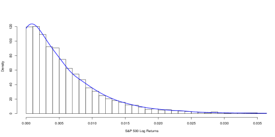
Figure 1: The histogram (using 150 bins) of the observed S&P 500 data and the kernel density plot (bandwidth = 0.001) of the simulated data using the obtained estimates.

5.1.2 Comparison between $gL(\alpha,\delta,\mu)$ and $gL(\alpha,1,\mu)$ distributions

We also analyzed the entire log adjusted closing returns ($n=17,025$). From the the estimates in Table 4, the estimates for $\delta$ favor values larger than one, which implies that the daily S&P 500 log returns (adjusted closing) are not adequately described by the two-parameter Linnik distribution ($\delta=1$). Note that we are not able to get an interval estimate for $\delta$ as the optim function gives the same value as a root for every bootstrap sample. The table also indicates that $\alpha$ is likely to be less than two and $\hat{\mu}$ is way larger than the estimate obtained in the preceding section. The two-parameter estimate of $\alpha$ exceeds two indicating a bad fit of the model to the data. But the estimates of $\mu$ from both two- and three-parameter models are comparable.

Table 4. Parameter estimates for $gL(\alpha,\delta,\mu)$ and $gL(\alpha,1,\mu)$ models applied to (S&P) 500 data.

$Estimator$	Point	$95\%$ CI	Point ($\delta=1$)	$95\%$ CI ($\delta=1$)
$\hat{\alpha}$	1.915	(1.881,  1.952)	2.445	(2.364,   2.529)
$\hat{\delta}$	1.23
$\hat{\mu}$	19115.36	(16255.82 ,  22675.40)	193059	(131357.3 ,   289028)

Figure 2 below confirms the good fit of the $gL(\alpha,\delta,\mu)$ family (using $2n=33798$ simulated observations) to the log adjusted closing returns. It also reveals that the flexibility of the proposed three-parameter $gL(\alpha,\delta,\mu)$ permits better capturing of the peak of the data at the origin. Note that the algorithm used in the calculation was not able to generate a comparable fit as $\hat{\alpha}$ is way larger than two (upper bound).

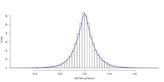
Figure 2: The histogram (using 150 bins) of the observed data and the kernel density plot (bandwidth = 0.001) of the simulated data using the obtained estimates superimposed on top.

5.2 Dow Jones Industrial Average index

The Dow Jones Industrial Average (DJIA) is a price-weighted average of 30 significant stocks traded on the New York Stock Exchange and the NASDAQ. The DJIA was invented by Charles Dow back in 1896. Often referred to as ”the Dow,” the DJIA is one of the oldest, single most-watched indices in the world and includes companies such as General Electric Company, the Walt Disney Company, Exxon Mobil Corporation and Microsoft Corporation. When the index was first launched, it included companies that were almost purely industrial in nature. The first components included railroads, cotton, gas, sugar, tobacco and oil companies. General Electric is the only one of the original Dow components that is still a part of the index in 2016. (Source: Investopedia)

5.2.1 Comparison between $gML(\alpha,\delta,\mu)$ and $gML(\alpha,1,\mu)$ distributions

The analysis here is similar to the one we carried out in the previous subsection and deals with the absolute values of the negative adjusted closing log returns($n=4,359$) from the Dow Jones index. The 95% CI for $\mu$ is between 154 and 173. The estimates of $\alpha$ strongly favor values less than unity. The point and interval estimates of $\delta$ indicate that $\delta>1,$ which implies superiority of the generalized $gML(\alpha,\delta,\mu)$ distribution for the absolute values of Dow daily Jones log returns over the $gML(\alpha,1,\mu)$ distribution. Observe that the $gML(\alpha,1,\mu)$ fit provides similar estimates for $\mu$ but not for $\alpha,$ and that its kernel density estimate is missing as $\hat{\alpha}$ exceeds one.

Table 5. Parameter estimates for $gML(\alpha,\delta,\mu)$ model applied to Dow Jones data.

$Estimator$	Point	$95\%$ CI	Point ($\delta=1$)	$95\%$ CI ($\delta=1$)
$\hat{\alpha}$	0.983	(0.974,   0.995 )	1.050	(1.036,   1.061)
$\hat{\delta}$	1.211	(1.153,  1.274)
$\hat{\mu}$	162.596	(153.578,   173.375)	165.952	(157.062,   174.868)

Again, as in the S&P 500 case discussed above, we constructed the graphs (using $2n=8,718$ simulated observations) to investigate the model adequacy. The smoothed density of the $gML(0.983,1.211,162.596)$ is in Figure 3 . It basically confirms what we have already observed above, that is, the three-parameter model provides more flexibility in capturing the peak of the ’cupping’ near the origin than the two-parameter Mittag-Leffler distributions.

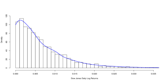
Figure 3: The histogram (using 150 bins) of the observed data and the kernel density plot (bandwidth = 0.001) of the simulated data using the obtained estimates superimposed on top.

5.2.2 Comparison between $gL(\alpha,\delta,\mu)$ and $gL(\alpha,1,\mu)$ distributions

We also applied the generalized Linnik distribution to the whole adjusted closings of the daily Dow Jones log returns ($n=17,025$). Looking at the estimate of $\delta,$ $\hat{\delta}>1$, it is clear that the daily Dow Jones log returns (using the adjusted closing) cannot be adequately described by the two-parameter Linnik distribution ($\delta=1$). Moreover, the table below shows $\alpha$ to be likely less than 1.9.

Table 6. Parameter estimates for $gL(\alpha,\delta,\mu)$ model applied to Dow Jones data.

$Estimator$	Point Estimate	$95\%$ CI	Point ($\delta=1$)	$95\%$ CI ($\delta=1$)
$\hat{\alpha}$	1.844	(1.803, 1.890)	2.258	(2.158, 2.366)
$\hat{\delta}$	1.24
$\hat{\mu}$	11762	( 9685 , 14605 )	63024	(39507 , 103585 )

Figure 4 shows the fits of the $gL(\alpha,\delta,\mu)$ and $gL(\alpha,\delta=1,\mu)$ models. Notice that the algorithm was able to produce a comparable fit in this case even if $\alpha>2.$ Furthermore, it validates the previous observation that the two-parameter $gL(\alpha,\delta=1,\mu)$ is not adequate for the description of the daily Dow Jones adjusted closing log returns especially in capturing the peak at the origin.

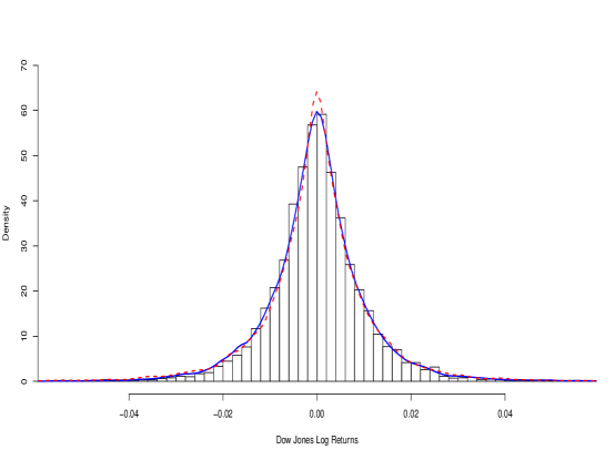
Figure 4: The histogram (using 150 bins) of the observed data and the kernel density plots (bandwidth = 0.001) of the simulated data (red dashed for 2-parameter $gL(\alpha,\delta=1,\mu)$ and solid blue for 3-parameter $gL(\alpha,\delta,\mu)$ ) using the obtained estimates.

6 Concluding remarks

The article proposes formal statistical inference procedures for the heavy-tailed three-parameter generalized Linnik and three-parameter generalized Mittag-Leffler families of distributions. The models provide considerable flexibility in modeling stationary discrete-time processes. The consistency and unbiasedness of the point estimators were computationally tested and seemed to be acceptable. Furthermore, the structural representations and the random number generation algorithms were provided for convenience. The paper provides guidance to how to distinguish different subcases of these models that exist in the literature.

The heavy-tailed three-parameter generalized Linnik and generalized Mittag-Leffler models present evidence that the adjusted S&P 500 and Dow Jones log returns can obey these probabilistic laws. The comparison of the proposed three-parameter models with the two-parameter models clearly demonstrated inadequacy of the latter ones especially when one considers approximations around the origin in modeling daily log returns of stock market data (see also Kozubowski, 2001).

Improvements of these procedures using robust, Bayesian approaches or more efficient algorithms, and the derivation of the trivariate or joint asymptotic distribution of the three point estimators would be worth exploring in the future.

References

- [1]
- [2] Abramowitz, M. Stegun, I., eds., Handbook of Mathematical Functions, National Bureau of Standards Applied Math.Series 55, Tenth Printing, USA, 1972.
- [3]
- [4] Anderson, D.N., A multivariate Linnik distribution, Statistics & Probability Letters, 14(4) (1992), 333–336.
- [5]
- [6] Anderson, D.N., Arnold, B.C., Linnik Distributions and Processes, Journal of Applied Probability, 30(2) (1993), 330–340.
- [7]
- [8] Arslan, O., An alternative multivariate skew Laplace distribution: properties and estimation, Statistical Papers, 30(2)(2008), DOI: 10.1007/s00362-008-0183-7.
- [9]
- [10] Bening, V.E., Korolev, V.Y., Kolokol’tsov, V.N., Saenko, V.V., Uchaikin, V.V., Zolotarev, V.V., Estimation of parameters of fractional stable distributions. Journal of Mathematical Sciences, 123(1)(2004), 3722–3732.
- [11]
- [12] Cahoy, D.O., An estimation procedure for the Linnik distribution. Statistical Papers, 53(3)(2012), 617–628.
- [13]
- [14] Cahoy, D.O., Estimation of Mittag-Leffler Parameters. Communications in Statistics - Simulation and Computation, 43(2)(2013), 303–315.
- [15]
- [16] Cahoy, D.O., Uchaikin, V.V., Woyczyński, W.A., Parameter estimation in fractional Poisson processes. Journal of Statistical Planning and Inference, 140(11),(2010) 3106–3120.
- [17]
- [18] Cahoy, D.O., Polito, F., Renewal processes based on generalized Mittag-Leffler waiting times. Communications in Nonlinear Science and Numerical Simulation, 18(3)(2013), 639–650.
- [19]
- [20] Chambers, J. M.; Mallows, C. L., Stuck, B. W., A method for simulating stable random variables, Journal of the American Statistical Association, 71(354)(1076), 340-344.
- [21]
- [22] Devroye, L., A note on Linnik’s distribution. Statistics & Probability Letters, 9(1990), 305–306.
- [23]
- [24] Jacques, C., Rmillard, B., Theodorescu, R. Estimation of Linnik law parameters, Statistics & Decisions, 17(3)(1999), 213–236.
- [25]
- [26] Gunaratnam, B., Woyczyǹski, W.A., Multiscale conservation laws driven by Lévy stable and Linnik diffusions: Asymptotics, shock creation, preservation and dissolution, J. Stat. Phys 56(2015), 1-33, DOI 10.1007/s10955-015-1240-y.
- [27]
- [28] Górska K., Woyczyński, W.A., Explicit representations for multiscale Lévy processes and asymptotics of multifractal conservation laws, J Math Phys, 56 (2015), 1-19, 083511 ; doi: 10.1063/1.4928047.
- [29]
- [30] Haan, L.D., Resnick, S.I., A simple asymptotic estimate for the index of a stable distribution, Journal of the Royal Stat’l Soc B, 42(1980), 83-87.
- [31]
- [32] Halvarsson, D., On the Estimation of Skewed Geometric Stable Distributions. Working Paper No. 216; Stockholm, Sweden: The Royal Institute of Technology, Division of Economics. 2013.
- [33]
- [34] Kanter, M., Stable densities under change of scale and total variation inequalities, The Annals of Probability, 3(4)(1975), 697-707.
- [35]
- [36] Klebanov, L.B., G.M. Maniya, I.A. Melamed, 1985. A problem of Zolotarev and analogs of infinitely divisible and stable distributions in a sheme for summing of a random number of random variables. Theory of Probability and its Applications, 29:4, 791–794.
- [37]
- [38] Kozubowski, T.J., Geometric stable laws: estimation and applications, Mathematical and Computer Modelling 29(1999), 241–253.
- [39]
- [40] Kozubowski, T.J., Fractional moment estimation of Linnik and Mittag-Leffler parameters, Mathematical and Computer Modelling 34 (2001), 1023–1035.
- [41]
- [42] Kotz, S., Ostrovskii, I.V., A mixture representation of the Linnik distribution, Statistics & Probability Letters, 26(1)(1996), 61–64.
- [43]
- [44] Kuttykrishnan, A.P., K. Jayakumar, K., Bivariate semi -Laplace distribution and processes, Statistical Papers, 49(2)(2006), 303–313.
- [45]
- [46] Laskin, N., Fractional Poisson process, Communications in Nonlinear Science and Numerical Simulation. 8 (3–4)(2003), 201–213.
- [47]
- [48] Leitch, R.A., Paulson, A.S., Estimation of stable law parameters: stock price behavior application. J. Amer. Statist. Assoc. 70(1975), 690–697.
- [49]
- [50] Lin, G.D., A note on the Linnik distributions, Journal of Mathematical Analysis and Applications, 217(1998), 701–706.
- [51]
- [52] Linnik, Yu.V., Linear forms and statistical criteria. I. II, Select Translat Math. Statist. Probab., 3(1963), 1–90.
- [53]
- [54] Pakes, A.G., Mixture representations for symmetric generalized Linnik laws, Statistical Probability Letters, 37(1998), 213–221.
- [55]
- [56] Paulson, A.S., Holcomb, E.W., Leitch, R.A., The estimation of the parameters of the stable laws. Biometrika 62(1975), 163–170.
- [57]
- [58] Pillai, R.N., 1990. On Mittag-Leffler distributions. Annals of the Institute of Statistical Mathematics, 42(1990), 157–161.
- [59]
- [60] Press, R.N. Estimation in univariate and multivariate stable distribution, J. Amer. Statist. Assoc., 67(1972), 842–846.
- [61]
- [62] Zolotarev, V.M., One-dimensional Stable Distributions: Translations of Mathematical Monographs, Vol 65, American Mathematical Society, 1986.
- [63]