On the band gap universality of multiphase laminates and its applications

Abstract

Shmuel and Band (2016) discovered that all infinite band structures of waves at normal incidence in two-phase laminates are encapsulated in a compact universal manifold. We show that manifolds of higher dimensionality encapsulate the band structures of all multiphase laminates. We use these manifolds to determine the density of gaps in the spectrum, and prove it is invariant with respect to certain properties. We further demonstrate that these manifolds are useful for formulating optimization problems on the gaps width, for which we develop a simple bound. Using our theory, we numerically study the dependency of the gaps density and width on the impedance and number of phases. Finally, we show that in certain settings, our analysis applies to non-linear multiphase laminates, whose band diagram is tunable by finite pre-deformations. Through simple examples, we demonstrate how the universality of our representation is useful for characterizing this tunability in multiphase laminates.

Keywords: Composite, Multiphase laminate, Bloch-Floquet analysis, Band gap, Phononic crystal, Wave propagation, Finite deformations

1 Introduction

Periodicity in a transmission medium for waves renders their propagation frequency dependent, even when the medium pointwise properties are not (Hussein et al., 2014). The resultant propagation can exhibit exotic or metamaterial characteristics, such as negative refraction and wave steering (Lu et al., 2009; Zelhofer and Kochmann, 2017). These phenomena are not only physically intriguing, but also have functional potential in applications such as cloaking and superlensing (Pendry, 2000; Milton et al., 2006; Colquitt et al., 2014).

Laminates—the media addressed in this paper—have the simplest periodicity, as their properties change only along one direction. Surprisingly, new results on their dynamics are still reported by ongoing research, e.g., metamaterial behavior of laminates (Bigoni et al., 2013; Nemat-Nasser, 2015; Willis, 2016; Srivastava, 2016), field patterns in laminates with time dependent moduli (Milton and Mattei, 2017), and dynamic homogenization of laminates (Nemat-Nasser and Srivastava, 2011; Nemat-Nasser et al., 2011; Herzig Sheinfux et al., 2014; Srivastava and Nemat-Nasser, 2014; Joseph and Craster, 2015).

We are concerned with the most familiar phenomenon: annihilation of waves at certain frequencies and corresponding emergence of a band-gap structure in the infinite spectrum (Sigalas and Economou, 1992; Kushwaha et al., 1993). The range of these gaps varies from one laminate to another, as function of the phase properties. For waves at normal incident angle, Shmuel and Band (2016) discovered that all band structures of laminates with two alternating layers are derived from a compact universal structure, independently of each layer thickness and specific physical properties. They used this universality to rigorously derive the maximal width, expected width, and density of the gaps, i.e., the relative width of the gaps within the entire spectrum. Finally, Shmuel and Band (2016) conjectured that such universality also exists for laminates made of an arbitrary number of phases. In what follows, we provide a rigorous proof for this conjecture, and employ it to answer several interesting questions, e.g., can the gap density be increased by adding more phases? If so, what are the optimal compositions that maximize it? Can we enlarge specific gaps in the same way?

The bulk of our analysis is presented in the framework of linear infinitesimal elasticity; in the sequel we show that in certain settings it extends to finite elasticity. Specifically, we show that our analysis applies for incremental waves propagating in non-linear multiphase laminates subjected to piecewise-constant finite deformations. Similarly to the case of finitely deformed two-phase laminates, the resultant band diagram is tunable by the static finite deformation (Shmuel and Band, 2016, cf., Zhang and Parnell, 2017); through simple examples, we demonstrate how the universality of our representation is useful for characterizing this tunability.

We present our results in the following order. Firstly, in Sec. 2 we revisit the derivation of the dispersion relation for multiphase laminates, from which the band structure is evaluated. Sec. 3 contains our theory; therein, we show that all infinite band structures of multiphase laminates are encapsulated in a compact universal manifold, whose dimensionality equals the number of layers in the periodic cell. We find that the gap density is the volume fraction of a universal submanifold, derive a closed-form expression for the submanifold boundary, and hence for the gap density. We further employ the new framework to provide a simple bound on the gaps width and formulate corresponding optimization problems. Sec. 4 employs our formulation to answer the questions posed earlier, via parametric investigation of the compact manifold. Sec. 5 details how our theory extends to non-linear multiphase laminates of tunable band diagrams, and demonstrates its application for characterizing this tunability. Finally, we summarize our results in Sec. 6.

2 Wave propagation in multiphase laminates

2.1 Dispersion relation

The solution to the problem of wave propagation in periodic laminates is well-known (Rytov, 1956); the topic receives renewed attention recently, owing to its applications in the context of metamaterials (Willis, 2016; Srivastava, 2016). For the reader convenience, this Sec. concisely recapitulates the formulation for multiphase laminates (Lekner, 1994), in the framework of linear elasticity.

A laminate is made of an infinite repetition of a unit cell comprising $N$ layers. We denote the thickness, mass density, and Lamé coefficients of the $n^{\mathrm{th}}$ layer by $h^{\left(n\right)},\rho^{\left(n\right)},\lambda^{\left(n\right)}$ and $\mu^{\left(n\right)}$, respectively. We consider plane waves propagating normal to the layers at frequency $\omega$. The equations of motion are satisfied by a displacement field which can be written in each layer as

$$\mathbf{u}^{\left(n\right)}=\mathbf{m}\left(A^{\left(n\right)}e^{ik^{\left(n\right)}\mathbf{n}\cdot\mathbf{x}}+B^{\left(n\right)}e^{-ik^{\left(n\right)}\mathbf{n}\cdot\mathbf{x}}\right)e^{-i\omega t},$$ (1)

where $\mathbf{n}$ is the lamination direction, $A^{\left(n\right)}$ and $B^{\left(n\right)}$ are constants, the wavenumber $k^{\left(n\right)}$ equals $\frac{\omega}{c^{\left(n\right)}}$, $c^{\left(n\right)}$ being the velocity that depends on the polarization $\mathbf{m}$, namely,

$$c^{\left(n\right)}=\sqrt{\frac{\tilde{\mu}^{\left(n\right)}}{\rho^{\left(n\right)}}}=\begin{cases}\begin{array}[]{cc}\sqrt{\frac{\mu^{\left(n\right)}}{\rho^{\left(n\right)}}},&\mathbf{m}\bot\mathbf{n},\\ \sqrt{\frac{\lambda^{\left(n\right)}+2\mu^{\left(n\right)}}{\rho^{\left(n\right)}}},&\mathbf{m}\|\mathbf{n}.\end{array}\end{cases}$$ (2)

It follows that $\mathbf{u}^{\left(n\right)}$ and the traction $\mathbf{t}^{\left(n\right)}$ at the borders of each layer are related via

$$\left\{\begin{array}[]{c}\mathbf{u}^{\left(n\right)}\left(\mathbf{x}+h^{\left(n\right)}\mathbf{n}\right)\\ \mathbf{t}^{\left(n\right)}\left(\mathbf{x}+h^{\left(n\right)}\mathbf{n}\right)\end{array}\right\}=\left[\begin{array}[]{cc}\cos k^{\left(p\right)}h^{\left(p\right)}&\frac{\sin k^{\left(p\right)}h^{\left(p\right)}}{\tilde{\mu}^{\left(n\right)}k^{\left(p\right)}}\\ -\tilde{\mu}^{\left(n\right)}k^{\left(p\right)}\sin k^{\left(p\right)}h^{\left(p\right)}&\cos k^{\left(p\right)}h^{\left(p\right)}\end{array}\right]\left\{\begin{array}[]{c}\mathbf{u}^{\left(n\right)}\left(\mathbf{x}\right)\\ \mathbf{t}^{\left(n\right)}\left(\mathbf{x}\right)\end{array}\right\}.$$ (3)

Invoking continuity conditions and sequentially applying Eq. (3) yields the following relation between the fields at the ends of the periodic cell

$$\left\{\begin{array}[]{c}\mathbf{u}^{\left(N\right)}\left(\mathbf{x}+h\mathbf{n}\right)\\ \mathbf{t}^{\left(N\right)}\left(\mathbf{x}+h\mathbf{n}\right)\end{array}\right\}=\prod_{n=1}^{N}\left[\begin{array}[]{cc}\cos k^{\left(p\right)}h^{\left(p\right)}&\frac{\sin k^{\left(p\right)}h^{\left(p\right)}}{\tilde{\mu}^{\left(n\right)}k^{\left(p\right)}}\\ -\tilde{\mu}^{\left(n\right)}k^{\left(p\right)}\sin k^{\left(p\right)}h^{\left(p\right)}&\cos k^{\left(p\right)}h^{\left(p\right)}\end{array}\right]\left\{\begin{array}[]{c}\mathbf{u}^{\left(1\right)}\left(\mathbf{x}\right)\\ \mathbf{t}^{\left(1\right)}\left(\mathbf{x}\right)\end{array}\right\},$$ (4)

where $h=\sum_{n=1}^{N}h^{\left(n\right)}$. Since the laminate is periodic and linear, we also have that (Kittel, 2005; Farzbod and Leamy, 2011)

$$\left\{\begin{array}[]{c}\mathbf{u}^{\left(N\right)}\left(\mathbf{x}+h\mathbf{n}\right)\\ \mathbf{t}^{\left(N\right)}\left(\mathbf{x}+h\mathbf{n}\right)\end{array}\right\}=e^{ik_{B}h}\left\{\begin{array}[]{c}\mathbf{u}^{\left(1\right)}\left(\mathbf{x}\right)\\ \mathbf{t}^{\left(1\right)}\left(\mathbf{x}\right)\end{array}\right\},$$ (5)

where $k_{B}$ is the Bloch wavenumber, quantifying the fields envelope. Eqs. (4-5) deliver the dispersion relation between $k_{B}$, $\omega$ and the properties of the layers, namely,

$$\eta=\cos k_{B}h,$$ (6)

where

$$\begin{split}\eta=&\prod_{n=1}^{N}\cos\frac{\omega h^{\left(n\right)}}{c^{\left(n\right)}}-\sum_{m=1}^{N-1}\sum_{n=m+1}^{N}\bigg{[}\gamma^{\left(n,m\right)}\Big{(}\prod_{k=m,n}\sin\frac{\omega h^{\left(k\right)}}{c^{\left(k\right)}}\Big{)}\prod_{l(\neq m,n)=1}^{N}\cos\frac{\omega h^{\left(l\right)}}{c^{\left(l\right)}}\bigg{]}+\\ &+\sum_{n=1}^{N-3}\sum_{p=n+2}^{N-1}\sum_{m=n+1}^{p-1}\sum_{q=p+1}^{N}\bigg{[}\gamma^{\left(n,m,p,q\right)}\Big{(}\prod_{k=m,n,p,q}\sin\frac{\omega h^{\left(k\right)}}{c^{\left(k\right)}}\Big{)}\prod_{l(\neq m,n,p,q)=1}^{N}\cos\frac{\omega h^{\left(l\right)}}{c^{\left(l\right)}}\bigg{]}+...,\end{split}$$ (7)

and

$$\left\{\gamma^{\left(n,m\right)}=\frac{1}{2}\left(\frac{\rho^{\left(n\right)}c^{\left(n\right)}}{\rho^{\left(m\right)}c^{\left(m\right)}}+\frac{\rho^{\left(m\right)}c^{\left(m\right)}}{\rho^{\left(n\right)}c^{\left(n\right)}}\right),\!\gamma^{\left(n,m,p,q\right)}=\frac{1}{2}\left(\frac{\rho^{\left(n\right)}c^{\left(n\right)}\rho^{\left(p\right)}c^{\left(p\right)}}{\rho^{\left(m\right)}c^{\left(m\right)}\rho^{\left(q\right)}c^{\left(q\right)}}+\frac{\rho^{\left(m\right)}c^{\left(m\right)}\rho^{\left(q\right)}c^{\left(q\right)}}{\rho^{\left(n\right)}c^{\left(n\right)}\rho^{\left(p\right)}c^{\left(p\right)}}\right),...\right\}\eqqcolon\left\{\gamma\right\}$$

quantifies the mismatch between the impedance of the phases and their combinations. Additional terms are added to Eq. (7) for $N>5$. We emphasize that these terms are of a similar form to the terms in Eq. (7), namely, products of $\cos\frac{\omega h^{\left(n\right)}}{c^{\left(n\right)}},\,\sin\frac{\omega h^{\left(n\right)}}{c^{\left(n\right)}}$, and impedance mismatch measures (Shen and Cao, 2000). The fact that $\eta$ maintains this functional form for arbitrary $N$ is central to our forthcoming analysis in Sec. 3.

2.2 Band structure and gap density

[figure]style=plain,subcapbesideposition=top

[]  []

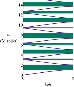
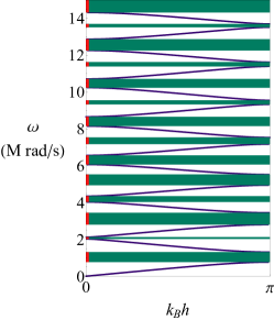
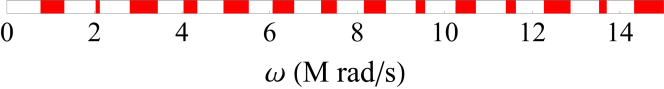
Figure 1: Representative band structures of 3-layer laminates. Panels (a) and (b) correspond to laminates (8) and (9), respectively. The truncated spectra, having the range of the gaps highlighted in red, are shown below the panels. The upper and lower spectra correspond to panels (a) and (b), respectively.

Waves at a frequency $\omega$ will propagate in the laminate only if Eq. (6) is satisfied by real $k_{B}$, and thus $\left|\eta\right|<1$. Otherwise, the Bloch parameter $k_{B}$ is imaginary and $\left|\eta\right|>1$, in which case the waves decay. The corresponding frequencies create gaps between propagating Bloch bands in the $k_{B}-\omega$ diagram, resulting in a band structure. It is clear from Eq. (6) that the band structure depends on the phase properties; it is also clear that the band structure is (generally) not periodic in $\omega$. Two representative band structures of 3-layer laminates are given in Fig. 1. Panel (a) corresponds to a laminate whose layer properties are

$$\begin{array}[]{lll}\rho^{\left(1\right)}=2700\,\mathrm{kg/m^{3}},&\mu^{\left(1\right)}=26\,\mathrm{GPa},&h^{\left(1\right)}=3\,\mathrm{mm},\\ \rho^{\left(2\right)}=8000\,\mathrm{kg/m^{3}},&\mu^{\left(2\right)}=80\,\mathrm{GPa},&h^{\left(2\right)}=2\,\mathrm{mm},\\ \rho^{\left(3\right)}=5000\,\mathrm{kg/m^{3}},&\mu^{\left(3\right)}=70\,\mathrm{GPa},&h^{\left(3\right)}=1.5\,\mathrm{mm}.\end{array}$$ (8)

The properties of layers 1 and 2 correspond to aluminum and steel, respectively, where layer 3 corresponds to a fictitious material whose impedance is between the impedance of layers 1 and 2. Panel (b) corresponds to a laminate layer properties are

$$\begin{array}[]{lll}\rho^{\left(1\right)}=4050\,\mathrm{kg/m^{3}},&\mu^{\left(1\right)}=39\,\mathrm{GPa},&h^{\left(1\right)}=5\,\mathrm{mm},\\ \rho^{\left(2\right)}=12000\,\mathrm{kg/m^{3}},&\mu^{\left(2\right)}=120\,\mathrm{GPa},&h^{\left(2\right)}=1\,\mathrm{mm},\\ \rho^{\left(3\right)}=7500\,\mathrm{kg/m^{3}},&\mu^{\left(3\right)}=105\,\mathrm{GPa},&h^{\left(3\right)}=4\,\mathrm{mm}.\end{array}$$ (9)

Note that the diagrams are truncated at $\omega=15\,\mathrm{M}\,\mathrm{rad/s}$; the truncated spectra, having the range of the gaps highlighted in red, are shown below the panels. The fact that $e^{ik_{B}h}=e^{i\left(k_{B}h+2\pi l\right)}$ for integer $l$, together with the symmetry of the $\cos$ function, implies that identify the gaps it is sufficient to evaluate $\omega$ against $0\leq k_{B}h\leq\pi$.

The density of the gaps, denoted $\varphi$, is their relative size in the frequency spectrum, i.e., the relative length of the sum of all red segments. We can define $\varphi$ more formally as follows. Let $\chi\left(\omega\right)$ denote the characteristic function

$$\chi\left(\omega\right)=\begin{cases}1&\omega\in\mathrm{gap},\\ 0&\mathrm{otherwise.}\end{cases}$$ (10)

In terms of $\chi,$ the relative size of the gaps in a frequency range $\left[0,\omega_{0}\right]$ is

$$\varphi_{\omega_{0}}=\frac{1}{\omega_{0}}\int_{0}^{\omega_{0}}\chi\left(\omega\right)\mathrm{d}\omega,$$ (11)

and the gap density is

$$\varphi\coloneqq\lim_{\omega_{0}\rightarrow\infty}\varphi_{\omega_{0}}.$$ (12)

Only recently, Shmuel and Band (2016) proved that for laminates made of two alternating layers the above limit exists, and provided an integral of a closed-form expression for its value, thus were able to calculate the gap density. The case of multilayer periodic cells case is next.

3 Universal gap structure in a compact manifold

Shmuel and Band (2016) found that all infinite band structures of two-layer laminates are encapsulated in a compact universal manifold, independent of the thickness of each layer and its specific physical properties; they further conjectured that this encapsulation can be generalized to an arbitrary number of layers. In the first part of this Sec., we prove this conjecture, derive a closed-form expression for the manifold that encapsulates the gap structure of multiphase laminates, and in turn, determine the corresponding gap density in terms of the manifold volume.

Shmuel and Band (2016) further recognized that the compact structure is also useful for formulating optimization problems on the gaps width, and derived simple bounds 2-layer laminates. In the second part of this Sec., we generalize their approach to multiphase laminates.

3.1 Morphism between spectral band gaps and the N-dimensional torus

Following the approach in Shmuel and Band (2016), we begin with the following substitution of variables

$$\zeta^{\left(n\right)}\coloneqq\frac{\omega h^{\left(n\right)}}{c^{\left(n\right)}},$$ (13)

which renders $\eta$ a $2\pi$-periodic function in each one of the new variables $\zeta^{\left(n\right)}$, i.e.,

$$\eta\left(\zeta^{\left(1\right)},\zeta^{\left(2\right)},...,\zeta^{\left(n\right)}+2\pi,...\zeta^{\left(N\right)};\left\{\gamma\right\}\right)=\eta\left(\zeta^{\left(1\right)},\zeta^{\left(2\right)},...,\zeta^{\left(n\right)},...\zeta^{\left(N\right)};\left\{\gamma\right\}\right).$$ (14)

This implies that the domain of $\eta$ can be represented by an N-dimensional torus whose coordinates are $\left(\zeta^{\left(1\right)},\zeta^{\left(2\right)},...,\zeta^{\left(N\right)}\right)$, such that each coordinate is defined modulo $2\pi$. The torus is equivalent to an N-dimensional cube, whose opposite sides are identified. In what follows, we interchange between the terms torus and cube, with the understanding that they are equivalent. The function $\eta$ linearly depends on $\sin\zeta^{\left(n\right)}$ and $\cos\zeta^{\left(n\right)}$, which change sign under the transformation $\zeta^{\left(n\right)}\rightarrow\zeta^{\left(n\right)}+\pi$, and hence $\eta$ changes sign too. It follows that $\left|\eta\right|$ is $\pi$-periodic in $\zeta^{\left(n\right)}$, hence defined over an N-dimensional torus, or N-cube, whose edges are of length $\pi$. Since the existence condition for Bloch waves depends on the absolute value of $\eta$, in what follows we focus on $\left|\eta\right|$ and the $\pi$-periodic torus. On this $\pi$-periodic torus, denoted $\mathbb{T}{}^{N}$, the equations $\frac{\mathrm{d}\zeta^{\left(n\right)}}{\mathrm{d}\omega\ ^{{\color[rgb]{1,1,1}n}}}=\frac{h^{\left(n\right)}}{c^{\left(n\right)}}$ define a linear flow $\left\{\overrightarrow{\zeta}\right\}_{\omega\in\mathbb{R}}$in the form

$$\overrightarrow{\zeta}\left(\omega\right)=\left(\frac{h^{\left(1\right)}}{c^{\left(1\right)}},\frac{h^{\left(2\right)}}{c^{\left(2\right)}},...,\frac{h^{\left(N\right)}}{c^{\left(N\right)}}\right)\omega\ \mathrm{mod}\ \pi.$$ (15)

The flow propagates uniformly in the N-cube as a line; we arbitrarily interpret $\zeta^{\left(N\right)}$ as the flow height, such that its slope in each one of the coordinates $\zeta^{\left(n\right)}$ is

$$a_{f}^{\left(n\right)}\coloneqq\frac{\zeta^{\left(N\right)}}{\zeta^{\left(n\right)}}=\frac{h^{\left(N\right)}}{c^{\left(N\right)}}\frac{c^{\left(n\right)}}{h^{\left(n\right)}}.$$ (16)

When the flow line reaches a cube face, it continues at the opposite one, owing to their identification. In the supplementary videos (available online), we present the morphism between the frequency axis in the band structure and the flow evolution on $\mathbb{T}{}^{3}$, for two laminates of different microstructure, and identical phased physical properties, given by Eq. (8).

If the slopes $\left\{a_{f}^{\left(n\right)}\right\}$ are rationally independent, viz., any set of integers $\left\{\alpha^{\left(n\right)}\right\}$ satisfies

$$\sum_{n=1}^{N}\alpha^{\left(n\right)}a_{f}^{\left(n\right)}\neq 0,$$ (17)

except the trivial set $\alpha^{\left(n\right)}=0$, then the flow covers the torus, as depicted by the supplementary videos. Furthermore, it implies that the linear flow is ergodic, such that averages over $\omega$ in the frequency domain are equivalent to averages over the torus. We are specifically interested in the gap density $\varphi$—the average of $\chi$, for which ergodicity implies

$$\varphi=\frac{1}{V}\int_{\mathbb{T}{}^{N}}\chi\left(\overrightarrow{\zeta}\right)\mathrm{d}V,$$ (18)

where $\mathrm{d}V=\mathrm{d}\zeta^{\left(1\right)}\mathrm{d}\zeta^{\left(2\right)}...\mathrm{d}\zeta^{\left(N\right)}$. We recall that $\chi$ equals 1 if a certain frequency belongs to a gap, which on the torus translates to the condition $\left|\eta\left(\overrightarrow{\zeta}\right)\right|>1$. In other words, gaps are identified with the intersection of the flow with a subset of the torus whose image is greater than 1; we denote this subset by $\mathbb{D}^{N}$. Hence, the gap density equals to the relative volume of this subset in the torus, namely,

$$\varphi=\frac{\mathrm{vol}\mathbb{D}^{N}}{\mathrm{vol}\mathbb{T}{}^{N}}.$$ (19)

We refer again to the supplementary videos, where $\mathbb{D}^{3}$ is depicted in green; since the laminates considered have the same $\left\{\gamma\right\}$, the gaps of the two flows are derived from the same $\mathbb{D}^{3}$; since the laminates microstructure is different, their flows differ in their direction.

For bilayer laminates, Shmuel and Band (2016) calculated the relative volume (area) by deriving a closed-form expression for the envelope (curve) of $\mathbb{D}^{2}$; we provide next a simple procedure to derive a closed-form expression for envelope of $\mathbb{D}^{N}$ for any $N$, i.e., when the unit cell comprises an arbitrary number of $N$ layers. The description of these hypersurfaces—on which

$$\left|\eta\right|=1,$$ (20)

requires an expression for $\zeta^{\left(N\right)}$ in terms of $\left\{\zeta^{\left(1\right)},...,\zeta^{\left(N-1\right)}\right\}$. To derive such expression, we define the variables

$$y_{n}\coloneqq\tan\frac{\zeta^{\left(n\right)}}{2},$$ (21)

and observe that in terms of $\left\{y_{n}\right\}$, the harmonic functions comprising $\left|\eta\right|$ are $\cos\zeta^{\left(n\right)}=\frac{1-y_{n}^{2}}{1+y_{n}^{2}}$ and $\sin\zeta^{\left(n\right)}=\frac{2y_{n}}{1+y_{n}^{2}}$. We multiply Eq. (20) by $1+y_{N}^{2}$, to obtain a quadratic equation for $y_{N}$, whose constants are combinations of $\left\{\gamma\right\}$, $\left(y_{1},...,y_{N-1}\right)$ and $\left(y_{1}^{2},...,y_{N-1}^{2}\right)$. Finally, by inverting Eq. (21) for $n=N$ and substituting the solution for $y_{N}$, we achieve a closed-form expression for $\zeta^{\left(N\right)}$. Accordingly for $\eta=-1$, we have that

$$\zeta^{\left(N\right)}=2\arctan\frac{-a_{1}\pm\sqrt{a_{1}^{2}-4a_{2}a_{0}}}{2a_{2}},$$ (22)

whose constants are

$$a_{0}=1,\ \ a_{1}=-2\gamma^{\left(1,2\right)}\tan\frac{\zeta^{\left(1\right)}}{2},\ \ a_{2}=\tan^{2}\frac{\zeta^{\left(1\right)}}{2},$$ (23)

when $N=2$; when $N=3$, the constants are

$$\begin{split}&a_{0}=\tan^{2}\frac{\zeta^{\left(1\right)}}{2}\tan^{2}\frac{\zeta^{\left(2\right)}}{2}-2\gamma^{\left(1,2\right)}\tan\frac{\zeta^{\left(1\right)}}{2}\tan\frac{\zeta^{\left(2\right)}}{2}+1,\\ &a_{1}=2\gamma^{\left(1,3\right)}\tan\frac{\zeta^{\left(1\right)}}{2}\left(\tan^{2}\frac{\zeta^{\left(2\right)}}{2}-1\right)+2\gamma^{\left(2,3\right)}\tan\frac{\zeta^{\left(2\right)}}{2}\left(\tan^{2}\frac{\zeta^{\left(1\right)}}{2}-1\right),\\ &a_{2}=\tan^{2}\frac{\zeta^{\left(1\right)}}{2}+\tan^{2}\frac{\zeta^{\left(2\right)}}{2}+2\gamma^{\left(1,2\right)}\tan\frac{\zeta^{\left(1\right)}}{2}\tan\frac{\zeta^{\left(2\right)}}{2},\\ \end{split}$$ (24)

and so on, for any $N$.

We conclude this part with remarks on laminates whose slopes $\left\{a_{f}^{\left(n\right)}\right\}$ are not rationally independent. The set of such laminates constitutes a subset with measure zero on the set of all possible laminates, since there are uncountably many rationally independent sets $\left\{a_{f}^{\left(n\right)}\right\}$, and countably many rationally dependent sets $\left\{a_{f}^{\left(n\right)}\right\}$. Therefore, this is a negligible set which corresponds to an irregular case, contrary to the generic case analyzed above, when the flow uniformly covers the whole torus. The only case in which the band diagram is periodic, and therefore also the orbit of the flow, is when all the slopes are rational numbers. Clearly, in this case the gap density is different than (19), and equals the relative length of the flow intersection with $\mathbb{D}$ over the length of one orbit. When $N=2$, the flow is either periodic or ergodic; when $N>2$, there exists the following additional scenario. Say only $a_{f}^{\left(m\right)}$ is rational and the remaining slopes are rationally independent. Then, the flow remains only on hyperplanes in the cube that are defined by $\zeta^{\left(N\right)}=\zeta^{\left(m\right)}a_{f}^{\left(m\right)}$, and covers uniformly only these hyperplanes. Similarly, if another slope is also rational, say $a_{f}^{\left(l\right)}$, then the flow remains on the intersection of hyperplanes defined by $\zeta^{\left(N\right)}=\zeta^{\left(m\right)}a_{f}^{\left(m\right)}$ and $\zeta^{\left(N\right)}=\zeta^{\left(l\right)}a_{f}^{\left(l\right)}$, covering it uniformly. This reduction of the flow orbit continues if additional slopes are rational, until the periodic case is obtained when all the slopes are rational numbers.

3.2 Gap width analysis on $\mathbb{T}{}^{N}$

Potential applications such as noise filters and vibration isolators require wide gaps; topology optimization aims at tailoring the medium microstructure to this objective (Sigmund and Søndergaard Jensen, 2003; Bilal and Hussein, 2011; Bortot et al., 2018). In this Sec., we employ our framework to formulate in a simple way these optimization problems on the compact manifold $\mathbb{D}^{N}$, and as a byproduct, derive a simple bound on the gaps width.

Our starting point is the identification of the gaps width on $\mathbb{T}{}^{N}$. Say the flow enters $\mathbb{D}^{N}$ at $\overrightarrow{\zeta}\left(\omega_{l}\right)=\left(\frac{h^{\left(1\right)}}{c^{\left(1\right)}},\frac{h^{\left(2\right)}}{c^{\left(2\right)}},...,\frac{h^{\left(N\right)}}{c^{\left(N\right)}}\right)\omega_{l}$, and exits at $\overrightarrow{\zeta}\left(\omega_{u}\right)=\left(\frac{h^{\left(1\right)}}{c^{\left(1\right)}},\frac{h^{\left(2\right)}}{c^{\left(2\right)}},...,\frac{h^{\left(N\right)}}{c^{\left(N\right)}}\right)\omega_{u}$. The distance between the two coordinates over the torus is

$$\Delta\zeta\coloneqq\left|\overrightarrow{\zeta}\left(\omega_{u}\right)-\overrightarrow{\zeta}\left(\omega_{l}\right)\right|=\Delta\omega\sqrt{\sum_{n=1}^{N}\frac{h^{\left(n\right)^{2}}}{c^{\left(n\right)^{2}}}},$$ (25)

where $\Delta\omega\coloneqq\omega_{u}-\omega_{l}$ is the gap width. (See Fig. 2(b) for an exemplary $\Delta\zeta$ segment of $\mathbb{D}^{3}$.) It follows that maximizing $\Delta\omega$ over an admissible set of unit cell compositions, denoted $\mathcal{S}\left(h^{\left(n\right)},c^{\left(n\right)}\right)$, is equivalent to maximizing $\Delta\zeta\left(\sum_{n=1}^{N}\frac{h^{\left(n\right)^{2}}}{c^{\left(n\right)^{2}}}\right)^{-\frac{1}{2}}$ over its corresponding admissible set. The merit in the expression that contains $\Delta\zeta$ is threefold. (i) It is formulated over the torus, hence encapsulates the whole spectra. (ii) Since we derived a closed-form expression for $\zeta^{\left(N\right)}$ in Eq. (15), at times a closed-form expression for $\Delta\zeta$ is accessible too. (iii) Eq. (25) lends itself for the basis of the following simple bound

$$\max_{\mathcal{S}\left(h^{\left(n\right)},c^{\left(n\right)}\right)}\Delta\omega=\max_{\mathcal{S}\left(a_{f}^{\left(n\right)},\overrightarrow{b}\right)}\left\{\Delta\zeta\left(\sum_{n=1}^{N}\frac{h^{\left(n\right)^{2}}}{c^{\left(n\right)^{2}}}\right)^{-\frac{1}{2}}\right\}\leq\max_{\mathcal{S}\left(a_{f}^{\left(n\right)},\overrightarrow{b}\right)}\left\{\Delta\zeta\right\}\,\max_{\mathcal{\mathcal{S}}\left(h^{\left(n\right)},c^{\left(n\right)}\right)}\left\{\left(\sum_{n=1}^{N}\frac{h^{\left(n\right)^{2}}}{c^{\left(n\right)^{2}}}\right)^{-\frac{1}{2}}\right\},$$ (26)

where $\mathcal{S}\left(a_{f}^{\left(n\right)},\overrightarrow{b}\right)$ is the corresponding set of admissible slops $a_{f}^{\left(n\right)}$ and intersection points $\overrightarrow{b}$ with the cube faces that characterize the linear flow lines. (Fig. 2(b) depicts such exemplary point $\overrightarrow{b}=\left(0,2,1.3\right)$ in $\mathbb{T}{}^{3}$.) In the sequel (Sec. 4.2), this analysis will be made more concrete via a specific optimization problem.

4 Parametric investigation on $\mathbb{T}{}^{N}$

4.1 Gap density analysis

[figure]style=plain,subcapbesideposition=top

[] [][]

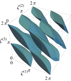
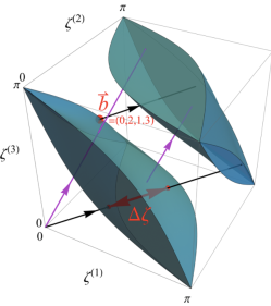
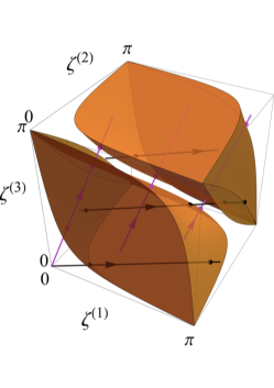
Figure 2: The envelope of $\mathbb{D}^{3}$ in the (a) 2$\pi$-periodic and (b) $\pi$-periodic cubes, of laminates with $\left\{\gamma\right\}=\{1.675,\ 1.34,\ 1.045\}$. Representative flow lines of laminates (8) and (27) are depicted in black and purple, respectively. (c) $\pi$-periodic envelope of $\mathbb{D}^{3}$ for laminates with $\left\{\gamma\right\}=\{6.76,\ 5.021,\ 1.045\}$. Part of two flows, when phase $1$ of laminate (8) is replaced by PMMA given in Eq. (28), with microstructures as in Eq. (29), are depicted in black and purple, respectively.

3-layer laminates. We begin with an analysis of 3-layer laminates, whose torus dimensionality enables its illustration. Fig. 2(a) shows the envelope of $\mathbb{D}^{3}$ in the 2$\pi$-cube of laminates with $\left\{\gamma\right\}\coloneqq\{\gamma^{\left(1,2\right)},\ \gamma^{\left(1,3\right)},\ \gamma^{\left(2,3\right)}\}=\{1.675,\ 1.34,\ 1.045\}$, e.g., laminate (8). Indeed, the structure is $\pi$-periodic, and the reduced $\pi$-periodic cube is depicted in Fig. 2(b). Therein, we also plot in black a part of the flow that corresponds to laminate (8). For comparison, a partial flow of a laminate with the same constituents, however with different thicknesses, namely,

$$\begin{array}[]{lll}h^{\left(1\right)}=1\,\mathrm{mm},&h^{\left(2\right)}=2\,\mathrm{mm},&h^{\left(3\right)}=3.5\,\mathrm{mm},\end{array}$$ (27)

is depicted in purple.

We illustrate the effect $\left\{\gamma\right\}$ has on the domain of $\mathbb{D}^{3}$ by replacing the first constituent of laminate (8) with PMMA, whose physical properties are

$$\begin{array}[]{ll}\rho^{\left(1\right)}=1180\,\mathrm{kg/m^{3}},&\mu^{\left(1\right)}=3\,\mathrm{GPa},\end{array}$$ (28)

and evaluating the resultant envelope in Fig. 2(c), which corresponds to $\left\{\gamma\right\}=\{6.76,\ 5.021,\ 1.045\}$. Parts of two representative flows, associated with the microstructures

$$\begin{array}[]{lll}h^{\left(1\right)}=3\,\mathrm{mm},&h^{\left(2\right)}=2\,\mathrm{mm},&h^{\left(3\right)}=1.5\,\mathrm{mm},\\ h^{\left(1\right)}=1\,\mathrm{mm},&h^{\left(2\right)}=2\,\mathrm{mm},&h^{\left(3\right)}=7.5\,\mathrm{mm},\\ \end{array}$$ (29)

are depicted in black and purple, respectively.

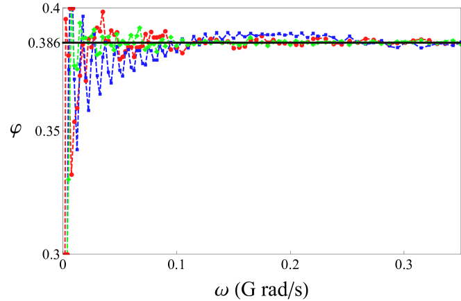
Figure 3: The gap density of laminates (8), (9) and (27), calculated on $\mathbb{T}{}^{3}$ (black line), and corresponding sequences $\varphi_{\omega_{0}}$, calculated directly from the original band structure (red and blue and green marks, respectively).

Fig. 3 compares the calculation of the gap density via Eq. (19) on $\mathbb{T}{}^{3}$ (black line), with sequences $\varphi_{\omega_{0}}$, calculated directly from the original band structure at increasing values of $\omega_{0}$. Specifically, we calculate the sequence for laminates (8) and (27), and denote its values at discrete $\omega_{0}$ by the red and blue marks, respectively. A third sequence (green marks) corresponds to laminate (9) whose properties are different from laminates (8) and (27), yet yield the same $\left\{\gamma\right\}$. Indeed, the sequences $\varphi_{\omega_{0}}$ converge to $\frac{\mathrm{vol}\mathbb{D}^{3}}{\mathrm{vol}\mathbb{T}{}^{3}}$, as our theory predicts.

[figure]style=plain,subcapbesideposition=top

[]  []

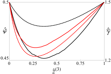
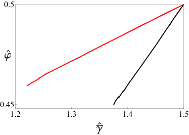
Figure 4: (a) Normalized gap density $\hat{\varphi}$ (continuous curves) and $\hat{\bar{\gamma}}$ (dashed curves) as functions of phase 3 normalized impedance. Black curves correspond to a laminate whose phases 1 and 2 impedance is as in (8). Red curves correspond to a laminate whose phase 1 (resp. 2) impedance is $2/3$ (resp. $3/2$) the impedance of phase 1 (resp. 2) in (8). (b) Normalized gap density as function of $\hat{\bar{\gamma}}$ .

The result that the gap density for classes of $\left\{\gamma\right\}$ is universal and computable via Eq. (18) is exploited next to investigate if we can increase the gap density of laminates of two alternating layers by introducing a third phase. To this end, in Fig. 4 we carry out a parametric investigation of the relation between the gap density, $\left\{\gamma\right\}$ and the impedance of the third phase, for a laminate whose phases 1 and 2 are as of laminate (8). Panel 4(a) shows the gap density (continuous black curves) and $\bar{\gamma}=\frac{\gamma^{\left(1,2\right)}+\gamma^{\left(1,3\right)}+\gamma^{\left(2,3\right)}}{3}$ (dashed black curves) as functions of phase 3 impedance, normalized according to

$$\begin{split}&\hat{z}^{\left(3\right)}\coloneqq\frac{z^{\left(3\right)}-z^{\left(1\right)}}{z^{\left(2\right)}-z^{\left(1\right)}},\\ &\hat{\varphi}\coloneqq 0.5\frac{\varphi}{\varphi(z^{\left(3\right)}=z^{\left(1\right)})},\\ &\hat{\bar{\gamma}}\coloneqq 1.5\frac{\bar{\gamma}}{\bar{\gamma}(z^{\left(3\right)}=z^{\left(1\right)})}.\end{split}$$ (30)

We observe that $\bar{\gamma}$ is smaller than its value for the bilayer laminate if the impedance of phase 3 is between the impedances of phases 1 and 2, and the value of the gap density is lower too. Conversely, if the impedance of phase 3 is greater (resp. lower) the the impedance of the phase 2 (resp. 1), the gap density is higher (not shown in the figure). We find that this trend is independent of the specific values of the impedance of phases 1 and 2. For example, we consider a laminate whose phase 1 (resp. 2) impedance is $2/3$ (resp. $3/2$) the impedance of phase 1 (resp. 2) in laminate (8). Its normalized gap density $\hat{\varphi}$ (red continuous curves) and $\hat{\bar{\gamma}}$ (red dashed curves) as functions of phase 3 impedance demonstrate the same trend. A different representation of this dependency is given in Fig. 4(b), in which the gap density is depicted versus $\hat{\bar{\gamma}}$. Indeed, we observe that the gap density is a monotonically increasing function of $\hat{\bar{\gamma}}$. We conclude that when subjected to the constraint

$$z^{\left(1\right)}<z^{\left(3\right)}<z^{\left(2\right)},$$ (31)

the gap density of 3-layer laminates cannot exceed the gap density of 2-layer laminates.

[figure]style=plain,subcapbesideposition=top

[]  []

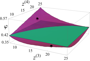
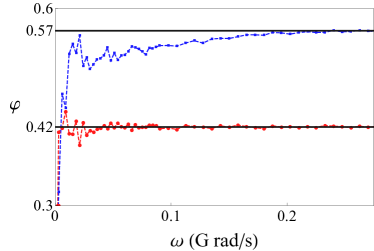
Figure 5: (a) Gap density as function of layers 3 and 4 impedance. Layers 1 and 2 impedance is as in (8)_1,2. The units of the $z^{\left(3\right)}$ and $z^{\left(4\right)}$ axes are $\mathrm{M}\,\mathrm{kg\,m^{-2}\,s^{-1}}$ (b) The $\varphi_{\omega_{0}}$ sequences of 2-layer laminate (red marks) with phases (8)_1,2 and microstructure (32), and a 4-layer laminate (blue marks) of the same phases, with microstructure (33). Corresponding values of the gap density calculated over $\mathbb{T}{}^{2}$ and $\mathbb{T}{}^{4}$, respectively, are given by black lines.

Laminates with 4 layers and more. Fig. 5(a) illustrates the gap density as function of layers 3 and 4 impedance, when layers 1 and 2 impedance is as in (8). As reference, the gap density of 2-layer laminates with the same $\gamma^{\left(1,2\right)}$ is represented by the green plane $\varphi=0.42$. A comparison with laminates whose unit cell comprises 3 layers shows two significant differences. (i) Here, the set $\left\{\gamma\right\}$ depends on the ordering of the phases, while for 3-layer laminates it does not. Specifically, $\gamma^{\left(1,2,3,4\right)}$ quantifies impedance mismatch of layers 1 and 3 versus layers 2 and 4. It follows that interchanging layers, except layers 1 and 3 or 2 and 4, changes $\gamma^{\left(1,2,3,4\right)}$ and, in turn, the gap density. Therefore, the bullet marked exemplary points $\left(10.07,20.22\right)$ and $\left(20.22,10.07\right)$ in Fig. 5 have different gap density. (ii) While the gap density of 2-layer laminates cannot be improved by introducing a third layer if $z^{\left(1\right)}<z^{\left(3\right)}<z^{\left(2\right)}$, it can be improved by introducing a fourth layer, even when $z^{\left(1\right)}<\left(z^{\left(3\right)},z^{\left(4\right)}\right)<z^{\left(2\right)}$. Interestingly, the optimal composition is when layers 3 and 4 are made of the phases that comprise layers 1 and 2, respectively, as it yields the greatest $\gamma^{\left(1,2,3,4\right)}$; of course, the thickness of layers 3 and 4 must be different than layers 1 and 2, and satisfy Eq. (17). This is demonstrated in Fig. 5(b) by evaluating two $\varphi_{\omega_{0}}$ sequences, associated with two laminates made of phases (8)_1,2, where one laminate is composed of 2 layers (red marks) with

$$\begin{array}[]{llll}h^{\left(1\right)}=3\,\mathrm{mm},&h^{\left(2\right)}=2\,\mathrm{mm},&&\\ \end{array}$$ (32)

and the other is composed of 4 layers (blue marks), with

$$\begin{array}[]{llll}h^{\left(1\right)}=1.3\,\mathrm{mm},&h^{\left(2\right)}=1.3\,\mathrm{mm},&h^{\left(3\right)}=1.7\,\mathrm{mm},&h^{\left(4\right)}=1.7\,\mathrm{mm}.\\ \end{array}$$ (33)

The corresponding calculations of the gap densities over $\mathbb{T}{}^{2}$ and $\mathbb{T}{}^{4}$, respectively, are given by the black lines. Indeed, we observe that the sequences converge to the theoretical values, and that the gap density of the 4-layer laminate is higher than the density of the 2-layer laminate.

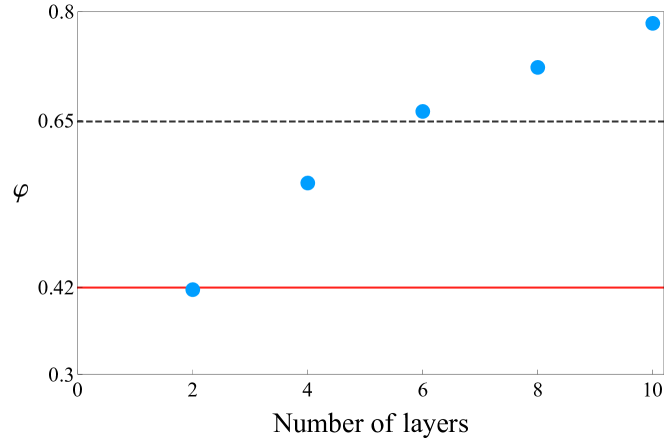
Figure 6: Gap density as function of the number of layers in a laminate made of phases 1 and 2 as in (8), where the two-layer gap density is shown also by the red solid line. The dashed line corresponds to a two-layer laminate whose phase 1 (resp. 2) impedance is $3/2$ (resp. $2/3$) the impedance of phase 1 (resp. 2) in (8).

Assuming the laminate is subjected to a constraint on the impedance range of available phases, our analysis suggests that the optimal scheme to increase the gap density is by adding pairs of layers made of the same two phases that constitute the 2-layer laminate, and varying their thickness. We illustrate this in Fig. 6, where the gap density is plotted against the number of layers in a laminate made of phases 1 and 2 as in (8)_1,2. As reference, the 2-layer case is also shown in red line. For comparison, the gap density of a 2-layer laminate whose phase 1 (resp. 2) impedance is $2/3$ (resp. $3/2$) the impedance of phase 1 (resp. 2) in (8) is shown in dashed line.

4.2 Maximization of the $1^{\mathrm{st}}$ gap

We apply next the general formulation in Sec. 3.2 to the address the following question. Consider two phases and the 2-layer microstructure that maximizes the $1^{\mathrm{st}}$ gap at a prescribed unit cell thickness $h$; can the $1^{\mathrm{st}}$ gap be widened by introducing a third layer made of a phase whose impedance is constrained between the impedances of the other two phases?

To answer the question, we first analyze the 2-layer case. The $1^{\mathrm{st}}$ gap corresponds to the segment originating at $\overrightarrow{b}=\overrightarrow{0}$. Since the phase properties and $h$ are prescribed, the optimization variable is only the thickness of one of the layers, say layer 1. Over the torus, this translates to optimization over the possible slopes $a_{f}^{\left(1\right)}$. Using the expression for $\mathbb{D}^{2}$ and its properties, we find that

$$\max_{a_{f}^{\left(1\right)}}\Delta\zeta=\Delta\zeta\left(a_{f}^{\left(1\right)}=1\right)=2\sqrt{2}\arctan\frac{\sqrt{\gamma+\sqrt{\gamma^{{}^{2}}-1}}-\sqrt{\gamma-\sqrt{\gamma^{2}-1}}}{2},$$ (34)

where $\gamma=\gamma^{\left(1,2\right)}$. The second part of the bound also admits an analytic solution, namely,

$$\max_{0<h^{\left(1\right)}<h}\left(\frac{h^{\left(1\right)^{2}}}{c^{\left(1\right)^{2}}}+\frac{\left(h-h^{\left(1\right)}\right)^{2}}{c^{\left(2\right)^{2}}}\right)^{-\frac{1}{2}}=\frac{\sqrt{c^{\left(1\right)^{2}}+c^{\left(2\right)^{2}}}}{h}$$ (35)

at $h^{\left(1\right)}=\frac{c^{\left(1\right)^{2}}}{c^{\left(1\right)^{2}}+c^{\left(2\right)^{2}}}h$, or in terms of the slope, at $a_{f}^{\left(1\right)}=\frac{c^{\left(2\right)}}{c^{\left(1\right)}}$, implying that the bound is sharp when the layers have the same phase velocity.[figure]style=plain,subcapbesideposition=top

[]  []

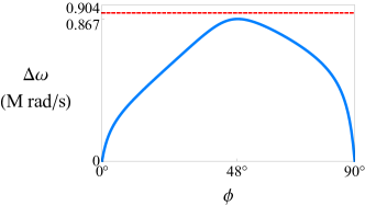
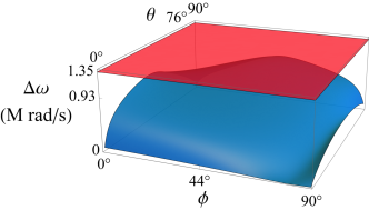
Figure 7: (a) $1^{\mathrm{st}}$ gap width as function of the $\theta$ (continuous blue curve), when phase 1 is (28), phase 2 is (8)₂, and $h=11.5\,\mathrm{mm}$. Our bound is depicted by the dashed red line. (b) $1^{\mathrm{st}}$ gap width (blue surface) as function of the possible microstructures of a 3-layer in terms of $\phi$ and $\theta$, whose phase properties are (28), (8)₂, and (38). Our bound is depicted by the red plane.

We analyze next the 3-layer case. We start with the second part of the bound. Given a third phase characterized by $c^{\left(3\right)}$, the analytic solution reads

$$\max_{\overset{h^{\left(1\right)},h^{\left(2\right)}}{\mathrm{s.t.}\ 0<h^{\left(1\right)}+h^{\left(2\right)}<h}}\left(\frac{h^{\left(1\right)^{2}}}{c^{\left(1\right)^{2}}}+\frac{h^{\left(2\right)^{2}}}{c^{\left(2\right)^{2}}}+\frac{\left(h-h^{\left(1\right)}-h^{\left(2\right)}\right)^{2}}{c^{\left(3\right)^{2}}}\right)^{-\frac{1}{2}}=\frac{\sqrt{c^{\left(1\right)^{2}}+c^{\left(2\right)^{2}}+c^{\left(3\right)^{2}}}}{h}$$ (36)

at $h^{\left(1\right)}=\frac{c^{\left(1\right)^{2}}}{c^{\left(1\right)^{2}}+c^{\left(2\right)^{2}}+c^{\left(3\right)^{2}}}h$ and $h^{\left(2\right)}=\frac{c^{\left(2\right)^{2}}}{c^{\left(1\right)^{2}}+c^{\left(2\right)^{2}}+c^{\left(3\right)^{2}}}h$, or in terms of the slopes, at $a_{f}^{\left(1\right)}=\frac{c^{\left(3\right)}}{c^{\left(1\right)}}$ and $a_{f}^{\left(1\right)}=\frac{c^{\left(3\right)}}{c^{\left(2\right)}}$. If the velocity $c^{\left(3\right)}$ is also a variable, the maximum is achieved at the greatest admissible $c^{\left(3\right)}$. We have employed a numerical analysis of $\mathbb{D}^{3}$ to find that $\max\Delta\zeta$ is along the diagonal of the face associated with the greatest $\gamma^{\left(n,m\right)}$, namely,

$$\max\Delta\zeta=2\sqrt{2}\max_{n,m}\left\{\arctan\frac{\sqrt{\gamma^{\left(n,m\right)}+\sqrt{\gamma^{\left(n,m\right)^{2}}-1}}-\sqrt{\gamma^{\left(n,m\right)}-\sqrt{\gamma^{\left(n,m\right)^{2}}-1}}}{2}\right\}.$$ (37)

We evaluate next the above results in the following numerical example. We set the properties of phase 1 to Eq. (28), phase 2 to Eq. (8)₂, and the unit cell thickness to $11.5\,\mathrm{mm}$. For these parameters, Eqs. (26), (34) and (35) provide the bound $0.9\mathrm{04M}\,\frac{\mathrm{rad}}{\mathrm{s}}$. Fig. 7(a) compares this bound (dashed red line) with the width as function of the polar angle $\phi$, where $\tan\phi=a_{f}^{\left(1\right)}$ (continuous blue curve). The optimal value, namely, $0.867\mathrm{M}\,\frac{\mathrm{rad}}{\mathrm{s}}$ at $\phi=48^{\circ}$, found to be very close to the bound. Consider a third phase whose properties are

$$\begin{array}[]{ll}\rho^{\left(3\right)}=3500\,\mathrm{kg/m^{3}}&\mu^{\left(3\right)}=55\,\mathrm{GPa,}\end{array}$$ (38)

such that its impedance is between the impedances of phases 1 and 2. Eqs. (26), (36) and (37) yield the bound $1.35\,\frac{\mathrm{rad}}{\mathrm{s}}$ on the $1^{\mathrm{st}}$ gap width when a third layer made of the latter phase is added. Fig. 7(b) compares this bound (red plane) with the width (blue surface) as function of the possible microstructures of the 3-layer in terms of $\phi$ and $\theta$, where $\tan\phi=\frac{a_{f}^{\left(1\right)}}{a_{f}^{\left(2\right)}}$ and $\tan\theta=\sqrt{\left(1/a_{f}^{\left(1\right)}\right)^{2}+\left(1/a_{f}^{\left(2\right)}\right)^{2}}$. The maximal width observed is $0.93\mathrm{M}\,\frac{\mathrm{rad}}{\mathrm{s}}$; indeed, as the change in the bound suggested, the $1^{\mathrm{st}}$ gap can be widened by introducing a third layer, even when its impedance is subjected to constraint (31).

5 Small-amplitude waves in finitely deformed multiphase laminates

Constitutively non-linear materials undergoing reversible large deformations attract growing attention, since they can comply with varying functional needs by virtue of their tunable geometrical and physical properties. Clearly, such materials can be useful when it is desirable to obtain tunable band diagrams, e.g., when the frequencies needed filtering are changing (Bertoldi and Boyce, 2008; Wang and Bertoldi, 2012; Getz and Shmuel, 2017; Barnwell et al., 2017; Ganesh and Gonella, 2017). The scheme for such tunability via finitely deformable multiphase laminates is simple, and we start with its informal description. The tuning mechanism is based upon an application of a finite quasi-static deformation, say, by an axial force, which results in a change of the thickness of each layer, and generally, its mass density. The constitutive behavior of the phases is non-linear, thus their instantaneous stiffness changes too. The propagation of small-amplitude waves depends on the above quantities, which are rendered tunable by the finite deformation; in turn, the band structure is rendered tunable too (Shmuel and deBotton, 2012).

Shmuel and Band (2016) employed the theory of incremental deformations superposed on large deformations (Ogden, 1997; Destrade and Saccomandi, 2007) to show that the dispersion relation of finitely deformed laminates made of two alternating layers is of the same functional form of Eq. (6) for $N=2$. Shmuel and Band (2016) further showed that the torus representation is applicable in this case too, and employed the compactness and universality of the torus to characterize the tunability. We concisely describe next the extension to finitely deformed multiphase laminates.

Consider again the laminate in Sec. 2, only now the unit cell comprises $N$ non-linear hyperelastic phases, whose stress is derived from functions $\Psi^{\left(n\right)}\left(\mathbf{F}\right)$ of the finite deformation gradient $\mathbf{F}$ via

$$\boldsymbol{\sigma}^{\left(n\right)}=\frac{1}{\det\mathbf{F}}\frac{\partial\Psi^{\left(n\right)}}{\partial\mathbf{F}}\mathbf{F}^{\mathrm{T}}.$$ (39)

In addition to the usual physical requirements on $\left\{\Psi^{\left(n\right)}\right\}$, we require symmetry with respect to the lamination direction $\mathbf{n}=\mathbf{e}_{3}$, but otherwise $\Psi^{\left(n\right)}$ are of general form. The laminate is quasi-statically deformed by applying an axial force of density $t_{A}$ per undeformed unit area. To determine the resultant deformation, the equations of continuity, far field conditions and equilibrium are to be satisfied. To this end, we postulate a piecewise homogeneous deformation, such that the deformation gradient matrix in layer $n$ is

$$\mathsf{F}^{\left(n\right)}=\mathrm{diag}\left[\lambda_{1}^{\left(n\right)},\lambda_{2}^{\left(n\right)},\lambda_{3}^{\left(n\right)}\right],$$ (40)

namely, unit cubes comprising layer $n$ are deformed to $\lambda_{1}^{\left(n\right)}\times\lambda_{2}^{\left(n\right)}\times\lambda_{3}^{\left(n\right)}$ cuboids. The outstanding quasi-static problem to determine $\left\{\lambda_{1}^{\left(n\right)},\lambda_{2}^{\left(n\right)},\lambda_{3}^{\left(n\right)}\right\}$ is addressed as follows. Firstly, the in-plane stretches in the different layers must match for the displacement field to be continuous across the interfaces, hence

$$\lambda_{2}^{\left(1\right)}=\lambda_{2}^{\left(2\right)}=...=\lambda_{2}^{\left(N\right)}\eqqcolon\lambda_{2},\lambda_{3}^{\left(1\right)}=\lambda_{3}^{\left(2\right)}=...=\lambda_{3}^{\left(N\right)}\eqqcolon\lambda_{3}.$$ (41)

The problem symmetry in the plane implies that

$$\lambda_{2}=\lambda_{3}\eqqcolon\lambda_{ip},$$ (42)

and equilibrium determines the remaining relations. Specifically, it leads to a constant axial stress throughout the laminate

$$\sigma_{11}^{\left(1\right)}=\sigma_{11}^{\left(2\right)}=...=\sigma_{11}^{\left(N\right)}=\frac{t_{A}}{\lambda_{ip}^{2}}.$$ (43)

Since the only force applied is axial, the remaining equation that completes the set of $N+1$ equations for the stretches $\left\{\lambda_{1}^{\left(n\right)}\right\}$ and $\lambda_{ip}$ is

$$\sum_{n=1}^{N}\lambda_{1}^{\left(n\right)}H^{\left(n\right)}\sigma_{22}^{\left(n\right)}=0,$$ (44)

where $H^{\left(n\right)}$ is the thickness of layer $n$ before the deformation. Note that for incompressible phases, the stretches are constrained via $\lambda_{ip}^{2}\lambda_{1}^{\left(n\right)}=1$, and a hydrostatic Lagrange multiplier is added to the stress. This completes the calculation of the laminate state in the deformed configuration.

To analyze small-amplitude wave propagation in the deformed laminate, a linearization is carried out about the deformed configuration. In each layer, we obtain a wave equation for the displacements $\mathbf{\mathbf{u}}^{\left(n\right)}\left(\mathbf{x},t\right)$ from the deformed state, namely,

$$\nabla\cdot\left(\boldsymbol{\mathcal{C}}^{\left(n\right)}\nabla\mathbf{u}^{\left(n\right)}\right)=\rho^{\left(n\right)}\ddot{\mathbf{u}}^{\left(n\right)},$$ (45)

where the instantaneous elasticities are

$$\mathcal{C}_{ijkl}^{\left(n\right)}=\frac{1}{\det\mathbf{F}^{\left(n\right)}}F_{j\alpha}^{\left(n\right)}\frac{\partial^{2}\Psi^{\left(n\right)}}{\partial F_{i\alpha}\partial F_{k\beta}}F_{l\beta}^{\left(n\right)}.$$ (46)

Note that the current mass densities $\left\{\rho^{\left(n\right)}\right\}$ depend on the finite deformation via $\rho^{\left(n\right)}=\rho^{\left(n\right)}_{0}/\det\mathbf{F}^{\left(n\right)}$, where $\rho^{\left(n\right)}_{0}$ is the initial mass density of phase $n$. It follows that Eq. (45) admits solutions in the form of Eq. (1), and the resultant continuity and Bloch-Floquet conditions reproduce Eq. (6), only now $\left\{h^{\left(n\right)},c^{\left(n\right)},\rho^{\left(n\right)}\right\}$ are functions of $t_{A}$. Since $\eta$ maintains its functional form, the arguments in Sec. (3) hold, hence the band structure of small-amplitude waves in finitely deformed multiphase laminates is also a linear flow on $\mathbb{T}{}^{N}$. The universality of the torus representation offers a convenient platform to analyze how the finite deformation affects the band structure, and replaces the need to carry out numerous evaluations of band structures at different deformations. This is demonstrated next, by way of examples.

To avoid cumbersome calculations, we focus on anti-plane shear waves, for which Eq. (45) simplifies to

$$\mathcal{C}_{2121}^{\left(n\right)}u_{2,11}^{\left(n\right)}=\rho^{\left(n\right)}\ddot{u}_{2}^{\left(n\right)}.$$ (47)

The resultant coordinates on the torus are

$$\zeta^{\left(n\right)}=\frac{\omega h^{\left(n\right)}}{c^{\left(n\right)}}=\frac{\omega\lambda^{\left(n\right)}_{1}H^{\left(n\right)}}{\sqrt{\hat{\mathcal{C}}_{2121}^{\left(n\right)}/\rho_{0}^{\left(n\right)}}},\ \left(\hat{\mathcal{C}}_{2121}^{\left(n\right)}=\det\mathbf{F}^{\left(n\right)}\mathcal{C}_{2121}^{\left(n\right)}\right)$$ (48)

with the slopes

$$a_{f}^{\left(n\right)}=\frac{\zeta^{\left(N\right)}}{\zeta^{\left(n\right)}}=\frac{h^{\left(N\right)}}{c^{\left(N\right)}}\frac{c^{\left(n\right)}}{h^{\left(n\right)}}=\frac{\lambda^{\left(N\right)}_{1}H^{\left(N\right)}}{\lambda^{\left(n\right)}_{1}H^{\left(n\right)}}\sqrt{\frac{\hat{\mathcal{C}}_{2121}^{\left(n\right)}\rho_{0}^{\left(N\right)}}{\hat{\mathcal{C}}_{2121}^{\left(N\right)}\rho_{0}^{\left(n\right)}}},$$ (49)

and the impedance contrasts that determine $\left\{\gamma\right\}$ are

$$\frac{z^{\left(m\right)}}{z^{\left(n\right)}}=\frac{\rho^{\left(m\right)}c^{\left(m\right)}}{\rho^{\left(n\right)}c^{\left(n\right)}}=\frac{\lambda_{1}^{\left(n\right)}}{\lambda_{1}^{\left(m\right)}}\sqrt{\frac{\hat{\mathcal{C}}_{2121}^{\left(m\right)}\rho_{0}^{\left(m\right)}}{\hat{\mathcal{C}}_{2121}^{\left(n\right)}\rho_{0}^{\left(n\right)}}}.$$ (50)

To continue, the form of $\left\{\Psi^{\left(n\right)}\right\}$ is needed. Assuming incompressible Gent phases (Gent, 1996), the finite deformation is homogeneous such that $\lambda^{\left(n\right)}_{1}=\lambda_{ip}^{-2}$, and the instantaneous shear moduli are

$$\hat{\mathcal{C}}_{2121}^{\left(n\right)}=\frac{\lambda_{ip}^{-4}\mu^{\left(n\right)}}{1-\frac{\lambda_{ip}^{-4}+2\lambda_{ip}^{2}-3}{J_{m}^{\left(p\right)}}};$$ (51)

here, $\mu^{\left(n\right)}$ is the shear modulus of phase $n$ in the limit of small strains, and $J_{m}^{\left(n\right)}\in(0,\infty]$ is a locking constant that models the stiffening of the material at finite strains. We now can demonstrate how the tunability affects the flow and $\mathbb{D}^{N}$ in $\mathbb{T}{}^{N}$, depending on the relations between the constants $\left\{\mu^{\left(n\right)},J_{m}^{\left(n\right)}\right\}$, through the following two representative cases.

• Case 1: $J_{m}^{\left(1\right)}=J_{m}^{\left(2\right)}=...=J_{m}^{\left(N\right)}\eqqcolon J_{m}$. Under this condition, the slopes $\left\{a_{f}^{\left(n\right)}\right\}$ are independent of the deformation, regardless of the relations between the shear moduli and mass densities. The impedance contrasts do not change either, hence $\mathbb{D}^{N}$ and $\varphi$ are invariant of the deformation. A change is identified in the flow rate $\frac{\mathrm{d}\overrightarrow{\zeta}}{\mathrm{d}\omega}$, which now multiplies the factor $\sqrt{1-\frac{\lambda_{ip}^{-4}+2\lambda_{ip}^{2}-3}{J_{m}}}$, and therefore the frequencies of each gap are divided by that factor. Since this factor is smaller than $1$ and approaches $0$ as the deformation becomes larger, the gaps are widened and shifted towards higher frequencies. Note that the limit $J_{m}\rightarrow\infty$ corresponds to neo-Hookean phases, whose analysis follows as a particular case, in which the flow rate does not change either.

• Case 2: $J_{m}^{\left(1\right)}\neq J_{m}^{\left(2\right)}\neq...\neq J_{m}^{\left(N\right)}$. Contrarily to the previous case, the layers stiffen at different rates. In turn, the slopes and impedance contrasts change in a way that depends on the relation between the different phase constants. There are numerous classes of relations between the constants; exploring them is outside our scope, however we provide an example for which the insights gained in Sec. 4 characterize certain aspects of the tunability. Our example considers 3-layer laminates, whose phase constants satisfy

  $$\mu^{\left(1\right)}=\mu^{\left(3\right)}<\mu^{\left(2\right)},\ J_{m}^{\left(3\right)}<J_{m}^{\left(1\right)}=J_{m}^{\left(2\right)},$$ (52)

  where, for simplicity, their mass density is equal. In the undeformed state, the band structure is identical to the band structure of a 2-layer laminate, encapsulated in $\mathbb{T}{}^{2}$ with $\gamma=\gamma^{\left(1,2\right)}$. Since $J_{m}^{\left(3\right)}<J_{m}^{\left(1\right)}$, the instantaneous stiffness and (consequently) impedance of layer 3 exceeds that of layer 1 upon deformation; up to a critical deformation, the resultant instantaneous impedances satisfy relation (31), with $\max_{n,m}\gamma^{\left(n,m\right)}$ fixed, and equal to $\gamma^{\left(1,2\right)}$. The band structure is described on $\mathbb{T}{}^{3}$, and our torus analysis in Sec. 4.1 shows that at fixed $\max_{n,m}\gamma^{\left(n,m\right)}$, the gap density in $\mathbb{T}{}^{3}$ is always lower than in $\mathbb{T}{}^{2}$ of the same $\gamma$. Thus, we deduce that the effect deformation has on the band structure is, on average, to narrow the gaps relatively to the undeformed state. At the critical deformation in which the strains are large enough to satisfy

  $$\frac{\lambda_{ip}^{-4}+2\lambda_{ip}^{2}-3-J_{m}^{\left(3\right)}}{\lambda_{ip}^{-4}+2\lambda_{ip}^{2}-3-J_{m}^{\left(2\right)}}\frac{J_{m}^{\left(2\right)}}{J_{m}^{\left(3\right)}}=\frac{\mu^{\left(3\right)}}{\mu^{\left(2\right)}},$$ (53)

  we have that $\gamma^{\left(1,3\right)}=\gamma^{\left(1,2\right)}$, hence the band structure is of a 2-layer laminate whose gap density equals the gap density of the undeformed laminate. Beyond this loading point, the instantaneous maximal impedance mismatch becomes greater than at lower strains. Our torus analysis in Sec. 4.1 indicates that, in turn, the resultant gap density is greater than the gap density at the undeformed state.

  

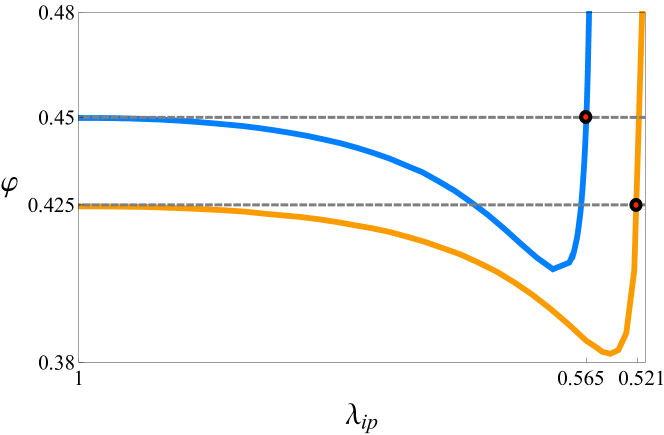
  Figure 8: Gap density as function of the pre-deformation parameter $\lambda_{ip}$, for the sets of materials . (54) and (55), depicted in blue and orange curves, respectively.

We conclude this Sec. with a numerical calculation demonstrating the latter result, considering 3-layer laminates whose properties are characteristic properties of elastomers (see, e.g., Getz et al., 2017, and the references therein). Specifically, the two laminates considered are given by

$$\begin{array}[]{lll}\rho^{\left(1\right)}=\rho^{\left(2\right)}=\rho^{\left(3\right)}=1000\,\mathrm{kg/m^{3}},\\ \mu^{\left(1\right)}=\mu^{\left(3\right)}=500,\ \mu^{\left(2\right)}=5500\,\mathrm{kPa},\\ J_{m}^{\left(1\right)}=J_{m}^{\left(2\right)}=35,\ J_{m}^{\left(3\right)}=8,\end{array}$$ (54)

and

$$\begin{array}[]{lll}\rho^{\left(1\right)}=\rho^{\left(2\right)}=\rho^{\left(3\right)}=1000\,\mathrm{kg/m^{3}},\\ \mu^{\left(1\right)}=\mu^{\left(3\right)}=650,\ \mu^{\left(2\right)}=6100\,\mathrm{kPa},\\ J_{m}^{\left(1\right)}=J_{m}^{\left(2\right)}=40,\ J_{m}^{\left(3\right)}=12.\end{array}$$ (55)

The gap density of laminates (54) and (55) as function of the pre-deformation parameter $\lambda_{ip}$ is depicted Fig. 8 by the blue and orange curves, respectively. Indeed, as our analysis implied, when the layers satisfy Eq. (52), pre-deformations reduce the gap density in comparison with the gap density of the undeformed laminates. At the critical deformation $\lambda_{ip}=0.565$, the instantaneous moduli of layers 2 and 3 in laminate (54) are equal, namely, $\hat{\mathcal{C}}_{2121}^{\left(2\right)}=\hat{\mathcal{C}}_{2121}^{\left(3\right)}=68.3\,\mathrm{MPa}$. Accordingly, at this deformation the gap density equals the gap density of the undeformed laminate, as indicated by the red dot in the plot. The maximal impedance mismatch beyond this point exceeds its counterpart at $\lambda_{ip}=1$, hence the gap density is greater than in the reference configuration. Laminate (55) undergoes a similar process, with the critical deformation $\lambda_{ip}=0.521$, at which $\hat{\mathcal{C}}_{2121}^{\left(2\right)}=\hat{\mathcal{C}}_{2121}^{\left(3\right)}=114.1\,\mathrm{MPa}$.

6 Summary

We have shown that the infinite band diagrams of waves at normal incident angle to N-phase laminates are encapsulated in a universal compact manifold, namely, $\mathbb{T}{}^{N}$, independently of the specific properties of the layers. The frequency parametrizes a linear flow over $\mathbb{T}{}^{N}$, whose intersection with the submanifold $\mathbb{D}^{N}$ is identified with gaps in the band diagrams. Using ergodicity arguments, we proved that the gap density of N-phase laminates is a well-defined quantity, universal for classes of laminates, and equals $\frac{\mathrm{vol}\mathbb{D}^{N}}{\mathrm{vol}\mathbb{T}{}^{N}}.$ This result was supplemented with numerical examples, demonstrating that the calculation of the gap density in the original band structures, truncated at increasing frequencies for different multiphase laminates, converges to the relative volume of $\mathbb{D}^{N}$.

We have employed our theory in a numerical study on the relation between the gap density, number of layers, and their impedance. Interestingly, we found that the gap density of two-layer laminates is increased by adding to the unit cell pairs of layers made of the same phases at different thicknesses. We have also showed that the encapsulation of the band diagrams in $\mathbb{T}{}^{N}$ is useful for formulating optimization problems on the gaps width, and developed a simple bound. By way of example, we addressed the question: can we enlarge the $1^{\mathrm{st}}$ gap of the optimal two-layer laminate by adding phases to the unit cell, even when the impedance of the added phases is constrained between the impedance of the original laminate phases? To this end, we have analytically calculated the bound for two-layer laminates, finding it is sharp. We have semi-analytically calculated the bound for the constrained 3-layer laminate, and found it is higher than the bound in the two-layer case, suggesting that the answer is yes. We have further evaluated the gap width as function of the microstructure for exemplary phases, using its expression over the torus in the two cases. Indeed, this evaluation confirmed that the optimal microstructure in the 3-layer case yields a wider $1^{\mathrm{st}}$ gap than the optimal microstructure in the two-layer case.

Finally, we have analyzed laminates comprising an arbitrary number of non-linear finitely deformed phases. We have showed that if such laminates undergo finite piecewise-constant deformations, the dispersion relation of superposed small-amplitude waves is similar to the dispersion relation of linear laminates, where the phase moduli and thickness become functions of the finite deformation. Hence, our theory and analysis of linear laminates extend to non-linear laminates under the foregoing settings. In addition, we have demonstrated how our framework facilitates the characterization of the band diagram tunability by static finite deformations.

We conclude this paper noting that our theory applies for additional multiphase systems, other than elastic laminates, whose dispersion relation is functionally similar to Eq. (6), e.g., certain electroelastic systems (Qian et al., 2004; Shmuel and deBotton, 2012) and stratified photonic crystals (Shmuel and Band, ), owing to the similarly with the problem of electromagnetic waves (Lekner, 1994; Adams et al., 2008).

References

- Adams et al. [2008] S.D.M. Adams, R.V. Craster, and S. Guenneau. Bloch waves in periodic multi-layered acoustic waveguides. Proceedings of the Royal Society of London A, 464(2098):2669–2692, 2008.
- Band and Berkolaiko [2013] Ram Band and Gregory Berkolaiko. Universality of the momentum band density of periodic networks. Physical Review Letters, 111:130404, 2013. doi: 10.1103/PhysRevLett.111.130404. URL http://link.aps.org/doi/10.1103/PhysRevLett.111.130404.
- Barnwell et al. [2017] E. G. Barnwell, W. J. Parnell, and I. D. Abrahams. Tunable elastodynamic band gaps. Extreme Mechanics Letters, 12:23–29, 2017. ISSN 2352-4316. doi: http://doi.org/10.1016/j.eml.2016.10.009. URL http://www.sciencedirect.com/science/article/pii/S2352431616300815. Frontiers in Mechanical Metamaterials.
- Barra and Gaspard [2000] F. Barra and P. Gaspard. On the level spacing distribution in quantum graphs. J. Statist. Phys., 101(1–2):283–319, 2000. doi: 10.1023/A:1026495012522.
- Bertoldi and Boyce [2008] K. Bertoldi and M.C. Boyce. Wave propagation and instabilities in monolithic and periodically structured elastomeric materials undergoing large deformations. Physical Review B, 78:184107, 2008. doi: 10.1103/PhysRevB.78.184107. URL http://link.aps.org/doi/10.1103/PhysRevB.78.184107.
- Bigoni et al. [2013] D. Bigoni, S. Guenneau, A. B. Movchan, and M. Brun. Elastic metamaterials with inertial locally resonant structures: Application to lensing and localization. Phys. Rev. B, 87:174303, May 2013. doi: 10.1103/PhysRevB.87.174303. URL https://link.aps.org/doi/10.1103/PhysRevB.87.174303.
- Bilal and Hussein [2011] O.R. Bilal and M.I. Hussein. Ultrawide phononic band gap for combined in-plane and out-of-plane waves. Physical Review E, 84:065701, 2011. doi: 10.1103/PhysRevE.84.065701.
- Bortot et al. [2018] E. Bortot, O. Amir, and G. Shmuel. Topology optimization of dielectric elastomers for wide tunable band gaps. accepted to International Journal of Solids and Structures, 2018.
- Colquitt et al. [2014] D.J. Colquitt, M. Brun, M. Gei, A.B. Movchan, N.V. Movchan, and I.S. Jones. Transformation elastodynamics and cloaking for flexural waves. Journal of the Mechanics and Physics of Solids, 72:131–143, 2014. ISSN 0022-5096. doi: http://dx.doi.org/10.1016/j.jmps.2014.07.014. URL http://www.sciencedirect.com/science/article/pii/S0022509614001586.
- Destrade and Saccomandi [2007] M. Destrade and G. Saccomandi, editors. Waves in nonlinear pre-stressed materials. CISM Course and Lectures. NY: Springer Wien, 2007.
- Farzbod and Leamy [2011] Farhad Farzbod and Michael J. Leamy. Analysis of bloch’s method and the propagation technique in periodic structures. Journal of Vibration and Acoustics, 133(3):031010–031010, 2011. URL http://dx.doi.org/10.1115/1.4003202.
- Ganesh and Gonella [2017] R. Ganesh and S. Gonella. Nonlinear waves in lattice materials: Adaptively augmented directivity and functionality enhancement by modal mixing. Journal of the Mechanics and Physics of Solids, 99:272–288, 2017. ISSN 0022-5096. doi: http://doi.org/10.1016/j.jmps.2016.11.001. URL http://www.sciencedirect.com/science/article/pii/S0022509616305440.
- Gent [1996] A. N. Gent. A new constitutive relation for rubber. Rubber Chem. Technol., 69:59–61, 1996.
- Getz et al. [2017] R. Getz, D.M. Kochmann, and G. Shmuel. Voltage-controlled complete stopbands in two-dimensional soft dielectrics. International Journal of Solids and Structures, 113–114:24–36, 2017. ISSN 0020-7683. doi: http://doi.org/10.1016/j.ijsolstr.2016.10.002. URL http://www.sciencedirect.com/science/article/pii/S0020768316302931.
- Getz and Shmuel [2017] Roey Getz and Gal Shmuel. Band gap tunability in deformable dielectric composite plates. International Journal of Solids and Structures, 128:11 – 22, 2017. ISSN 0020-7683. doi: https://doi.org/10.1016/j.ijsolstr.2017.07.021. URL http://www.sciencedirect.com/science/article/pii/S0020768317303384.
- Herzig Sheinfux et al. [2014] Hanan Herzig Sheinfux, Ido Kaminer, Yonatan Plotnik, Guy Bartal, and Mordechai Segev. Subwavelength multilayer dielectrics: Ultrasensitive transmission and breakdown of effective-medium theory. Physical Review Letters, 113:243901, 2014. doi: 10.1103/PhysRevLett.113.243901. URL https://link.aps.org/doi/10.1103/PhysRevLett.113.243901.
- Hussein et al. [2014] M.I. Hussein, M.J. Leamy, and M. Ruzzene. Dynamics of phononic materials and structures: Historical origins, recent progress, and future outlook. Applied Mechanics Reviews, 66(4):040802–040802, 05 2014. URL http://dx.doi.org/10.1115/1.4026911.
- Joseph and Craster [2015] L.M. Joseph and R.V. Craster. Reflection from a semi-infinite stack of layers using homogenization. Wave Motion, 54:145 – 156, 2015. ISSN 0165-2125. doi: https://doi.org/10.1016/j.wavemoti.2014.12.003. URL http://www.sciencedirect.com/science/article/pii/S0165212514001747.
- Katok and Hasselblatt [1996] A. Katok and B. Hasselblatt. Introduction to the modern theory of dynamical systems. Cambridge, 1996.
- Kittel [2005] C. Kittel. Introduction to Solid State Physics. John Wiley & Sons, Inc., Hoboken, NJ, 2005.
- Kohmoto et al. [1983] Mahito Kohmoto, Leo P. Kadanoff, and Chao Tang. Localization problem in one dimension: Mapping and escape. Phys. Rev. Lett., 50:1870–1872, Jun 1983. doi: 10.1103/PhysRevLett.50.1870. URL https://link.aps.org/doi/10.1103/PhysRevLett.50.1870.
- Kushwaha et al. [1993] M.S. Kushwaha, P. Halevi, L. Dobrzynski, and B. Djafari-Rouhani. Acoustic band structure of periodic elastic composites. Physical Review Letters, 71(13):2022–2025, 1993.
- Lekner [1994] John Lekner. Light in periodically stratified media. J. Opt. Soc. Am. A, 11(11):2892–2899, Nov 1994. doi: 10.1364/JOSAA.11.002892. URL http://josaa.osa.org/abstract.cfm?URI=josaa-11-11-2892.
- Lu et al. [2009] M.-H. Lu, L. Feng, and Y.-F. Chen. Phononic crystals and acoustic metamaterials. Materials Today, 12(12):34 – 42, 2009. ISSN 1369-7021. doi: https://doi.org/10.1016/S1369-7021(09)70315-3. URL http://www.sciencedirect.com/science/article/pii/S1369702109703153.
- Milton and Mattei [2017] Graeme W. Milton and Ornella Mattei. Field patterns: a new mathematical object. Proceedings of the Royal Society of London A: Mathematical, Physical and Engineering Sciences, 473(2198), 2017. ISSN 1364-5021. doi: 10.1098/rspa.2016.0819. URL http://rspa.royalsocietypublishing.org/content/473/2198/20160819.
- Milton et al. [2006] G.W. Milton, M. Briane, and J.R. Willis. On cloaking for elasticity and physical equations with a transformation invariant form. New Journal of Physics, 8(10):248, 2006. URL http://stacks.iop.org/1367-2630/8/i=10/a=248.
- Nemat-Nasser and Srivastava [2011] S. Nemat-Nasser and A. Srivastava. Overall dynamic constitutive relations of layered elastic composites. Journal of the Mechanics and Physics of Solids, 59(10):1953–1965, 2011. ISSN 0022-5096. doi: http://dx.doi.org/10.1016/j.jmps.2011.07.008. URL http://www.sciencedirect.com/science/article/pii/S0022509611001475.
- Nemat-Nasser et al. [2011] S. Nemat-Nasser, J. R. Willis, A. Srivastava, and A. V. Amirkhizi. Homogenization of periodic elastic composites and locally resonant sonic materials. Phys. Rev. B, 83:104103, Mar 2011. doi: 10.1103/PhysRevB.83.104103. URL https://link.aps.org/doi/10.1103/PhysRevB.83.104103.
- Nemat-Nasser [2015] Sia Nemat-Nasser. Anti-plane shear waves in periodic elastic composites: band structure and anomalous wave refraction. Proceedings of the Royal Society of London A: Mathematical, Physical and Engineering Sciences, 471(2180), 2015. ISSN 1364-5021. doi: 10.1098/rspa.2015.0152. URL http://rspa.royalsocietypublishing.org/content/471/2180/20150152.
- Ogden [1997] R.W. Ogden. Non-Linear Elastic Deformations. Dover Publications, New York, 1997.
- Pendry [2000] J. B. Pendry. Negative refraction makes a perfect lens. Phys. Rev. Lett., 85:3966–3969, Oct 2000. doi: 10.1103/PhysRevLett.85.3966. URL https://link.aps.org/doi/10.1103/PhysRevLett.85.3966.
- Qian et al. [2004] Z. Qian, F. Jin, Z. Wang, and K. Kishimoto. Dispersion relations for sh-wave propagation in periodic piezoelectric composite layered structures. International Journal of Engineering Science, 42(7):673 – 689, 2004. ISSN 0020-7225. doi: http://dx.doi.org/10.1016/j.ijengsci.2003.09.010. URL http://www.sciencedirect.com/science/article/pii/S002072250400014X.
- Rytov [1956] S. Rytov. Acoustical properties of a thinly laminated medium. Sov. Phys. Acoust., 2:68–80, 1956.
- Shen and Cao [2000] M. Shen and W. Cao. Acoustic bandgap formation in a periodic structure with multilayer unit cells. Journal of Physics D: Applied Physics, 33(10):1150, 2000. URL http://stacks.iop.org/0022-3727/33/i=10/a=303.
- [35] G. Shmuel and R. Band. Spectral statistics of layered photonic crystals are universal. In preparation.
- Shmuel and Band [2016] G. Shmuel and R. Band. Universality of the frequency spectrum of laminates. Journal of the Mechanics and Physics of Solids, 92:127 – 136, 2016. ISSN 0022-5096. doi: http://dx.doi.org/10.1016/j.jmps.2016.04.001.
- Shmuel and deBotton [2012] G. Shmuel and G. deBotton. Band-gaps in electrostatically controlled dielectric laminates subjected to incremental shear motions. Journal of the Mechanics and Physics of Solids, 60:1970–1981, 2012.
- Sigalas and Economou [1992] M. M. Sigalas and E. N. Economou. Elastic and acoustic wave band structure. Journal of Sound and Vibrations, 158(2):377 – 382, 1992.
- Sigmund and Søndergaard Jensen [2003] O. Sigmund and J. Søndergaard Jensen. Systematic design of phononic band–gap materials and structures by topology optimization. Philosophical Transactions of the Royal Society of London A: Mathematical, Physical and Engineering Sciences, 361(1806):1001–1019, 2003. doi: 10.1098/rsta.2003.1177.
- Srivastava [2016] A. Srivastava. Metamaterial properties of periodic laminates. Journal of the Mechanics and Physics of Solids, 96:252 – 263, 2016. ISSN 0022-5096. doi: http://dx.doi.org/10.1016/j.jmps.2016.07.018. URL http://www.sciencedirect.com/science/article/pii/S0022509616303933.
- Srivastava and Nemat-Nasser [2014] A. Srivastava and S. Nemat-Nasser. On the limit and applicability of dynamic homogenization. Wave Motion, 51(7):1045 – 1054, 2014. ISSN 0165-2125. doi: https://doi.org/10.1016/j.wavemoti.2014.04.003. URL http://www.sciencedirect.com/science/article/pii/S0165212514000614.
- Wang and Bertoldi [2012] L. Wang and K. Bertoldi. Mechanically tunable phononic band gaps in three-dimensional periodic elastomeric structures. International Journal of Solids and Structures, 49(19-20), 2012. doi: 10.1016/j.ijsolstr.2012.05.008.
- Willis [2016] J.R. Willis. Negative refraction in a laminate. Journal of the Mechanics and Physics of Solids, 97:10–18, 2016. ISSN 0022-5096. doi: http://dx.doi.org/10.1016/j.jmps.2015.11.004. URL http://www.sciencedirect.com/science/article/pii/S0022509615302623. SI:Pierre Suquet Symposium.
- Zelhofer and Kochmann [2017] A.J. Zelhofer and D.M. Kochmann. On acoustic wave beaming in two-dimensional structural lattices. International Journal of Solids and Structures, 115-116:248–269, 2017. ISSN 0020-7683. doi: http://doi.org/10.1016/j.ijsolstr.2017.03.024. URL http://www.sciencedirect.com/science/article/pii/S0020768317301336.
- Zhang and Parnell [2017] Pu Zhang and William J. Parnell. Soft phononic crystals with deformation-independent band gaps. Proceedings of the Royal Society of London A: Mathematical, Physical and Engineering Sciences, 473(2200), 2017. ISSN 1364-5021. doi: 10.1098/rspa.2016.0865. URL http://rspa.royalsocietypublishing.org/content/473/2200/20160865.