Quark model estimate of hidden-charm pentaquark resonances

Abstract

A quark model, which reproduces the ground-state mesons and baryons, i.e., the threshold energies, is applied to the $qqqc\bar{c}$ configurations, where $q$ is a light quark and $c$ the charmed quark. In the calculation, several open channels are explicitly included such as ${J/\psi}+N$, $\eta_{c}+N$, $\Lambda_{c}+D$, etc. To distinguish genuine resonances and estimate their width, we employ Gaussian Expansion Method supplemented by the real scaling method (stabilization). No resonance is found at the energies of the $P_{c}(4380)$ and $P_{c}(4450)$ pentaquarks. On the other hand, there is a sharp resonant state at 4690 MeV with $J=1/2^{-}$ state and another one at 4920 MeV with $J=3/2^{-}$ state, which have a compact structure.

I Introduction

During the past decades, several experimental candidates have been proposed for hadrons beyond the ordinary quark-antiquark and three-quark structures: baryonium, supernumerary scalar mesons, light pentaquarks, etc. However, most of them have not been confirmed in experiments with high statistics and better resolution, or their interpretation as multiquarks has a little faded away. A new era has begun with the discovery of the $X(3872)$ in 2003 Choi:2003ue and several other $XYZ$ states with hidden charm. Another striking result is the observation of the $P_{c}$ pentaquarks by the LHCb collaboration Aaij:2015tga . For a review, see for instance Hosaka:2016pey ; Chen:2016qju ; Richard:2016eis ; Lebed:2016hpi ; Karliner:2017qhf . It is now widely accepted that the spectrum of hadrons is not restricted to the excitations of ordinary mesons and baryons, and extends to multiquark configurations with hidden or open flavor.

Concerning the hidden-charm pentaquarks, there are many theoretical approaches: quark model approaches with different interactions Yuan:2012wz ; Santopinto:2016pkp ; Wu:2017weo , quark-cluster model Takeuchi:2016ejt , diquark models Maiani:2015vwa ; Li:2015gta ; Ali:2016dkf ; Lebed:2015tna ; Zhu:2015bba ; Zhu:2015bba , and hadronic molecular picture Wu:2010jy ; Wu:2010vk ; Garcia-Recio:2013gaa ; Karliner:2015ina ; Chen:2015loa ; Roca:2015dva ; He:2015cea ; Meissner:2015mza ; Chen:2015moa ; Uchino:2015uha ; Shimizu:2016rrd ; Yamaguchi:2016ote ; Shimizu:2017xrg . The observation channel consists of a proton and a ${J/\psi}$, suggesting as quark content $c\bar{c}$ attached to light quarks. In the hadronic molecular description, the $P_{c}$ states couple to both open charm and hidden charm hadrons in channels such as ${J/\psi}\,p$ or $\bar{D}\Sigma_{c}$, and hence whatever dynamical scheme is adopted at start, the detailed properties are sensitive to all surrounding thresholds and their interactions.

Within the quark-model picture, the technical aspect of this competition between multiquark and hadron-hadron components deals with finding a reliable solution of the model in the continuum. In the literature on the quark model (including by some of us), the bound-state formalism has often been used without caution for states in the continuum. To be more specific, if a crude trial wave function gives for some multiquark configuration an energy $E=-100\,$MeV below the lowest threshold, it is not too far from the exact solution within this model. On the other hand, an energy $E=+100\,$MeV above one of the thresholds might be meaningless. Refining the trial wave function should lead to convergence towards the lowest threshold. Identifying a resonance within a given model requires dedicated methods. One of such methods is the technique of real scaling along the fall-apart coordinate, starting from a rich variational function that includes several types of clustering.

In Ref. Hiyama:2005cf , two of the present authors (E.H. and A.H.) studied the $\Theta^{+}$ state as a $udds\bar{s}$ five-body problem, taking explicitly into account the $K\,N$ scattering channel. This was, to our knowledge, the first application of real scaling to a quark model calculation. The present article is devoted to the hidden-charm pentaquarks $P_{c}$, treated as a $uudc\bar{c}$ system, with account for all possible open channels such as $\Lambda_{c}+D^{*}$, $\Sigma_{c}+D$, $\Sigma_{c}^{*}+D$, etc. This is a rather delicate and lengthy calculation, but rather rewarding: most states appear as building a mere discretization of the continuum, but there are some striking exceptions which can be identified as genuine resonances in the model.

The paper is organized as follows. In Sec. II we present Hamiltonian and the method. The results are displayed and discussed in Sec. III. Finally we summarize our findings in Sec. IV.

II Hamiltonian and method

The Hamiltonian, which corresponds to a standard non-relativistic quark model, is given by

$$H=\sum_{i}(m_{i}+\frac{\boldsymbol{p}^{2}_{i}}{2m_{i}})-T_{G}-\frac{3}{16}\sum_{i<j}\lambda_{i}.\lambda_{j}\,V_{ij}(r_{ij}),$$ (1)

where $m_{i}$ and $\boldsymbol{p}_{i}$ are the mass and momentum of the $i^{\rm th}$ quark, $\lambda_{i}$ represents the eight color-SU(3) operators for the $i^{\rm th}$ quark and $T_{G}$ is the kinetic energy of the center-of-mass system. Here, we label the light quarks, $u$ and $d$, by $i=1$ to $3$, and heavy (charm) quarks, $c$ by $i=4$ and $\bar{c}$ by $i=5$.

For the quark-quark interaction, we use the potentials proposed by Semay and Silvestre-Brac Semay:1994ht ; Silvestre . The functional form of the potential in the $r$-space is given by

$$V_{ij}(r)=-\frac{\kappa}{r}+\lambda r^{p}-\Lambda\\ {}+\frac{2\pi\kappa^{\prime}}{3m_{i}m_{j}}\frac{\exp(-r^{2}/r_{0}^{2})}{\pi^{3/2}\,r^{3}_{0}}\,\boldsymbol{\sigma}_{i}.\boldsymbol{\sigma}_{j}\,,$$ (2)

where the smearing parameter $r_{0}$ is a function of the quark masses, $r_{0}(m_{i},m_{j})=A(\frac{2m_{i}m_{j}}{m_{i}+m_{j}})^{-B}$. Two sets of parameter choices, AP1 and AL1, are employed in the current analysis and listed in Table I.

Table 1: Parameters of AP1 and AL1 defined by Eq. (2.2).

	$p$	$m_{u,d}$(GeV)	$m_{s}$(GeV)	$\Lambda$(GeV)	$B$	$A$(GeVB-1)	$\kappa$	$\kappa$’	$\lambda$(GeV5/3)
AP1	$3/2$	0.277	0.553	1.851	0.3263	1.5296	0.5871	1.8025	0.3898
AL1	$1$	0.315	0.577	1.836	0.2204	1.6553	0.5069	1.8609	0.1653

Both sets reproduce rather well the masses of the ground states of heavy meson and baryon systems. In Table 2, the calculated spectra using AP1 are listed. The mass spectrum by AL1 is almost identical to that by AP1.

Table 2: The calculated masses (in MeV) of the heavy mesons and baryons entering the thresholds together with the experimental values.

hadron	$J^{P}$	cal.	exp.
$\eta_{c}$	$0^{-}$	2984	2983
${J/\psi}$	$1^{-}$	3103	3096
$D$	$0^{-}$	1882	1869
$D^{*}$	$1^{-}$	2033	2007
$N$	$1/2^{+}$	937	938
$\Lambda_{c}$	$1/2^{+}$	2290	2286
$\Sigma_{c}$	$1/2^{+}$	2472	2455
$\Sigma_{c}^{*}$	$3/2^{+}$	2545	2520

The five-body Schrödinger equation

$$(H-E)\Psi_{JM}=0\,$$ (3)

corresponding to the Hamiltonian (1) is solved by using the Gaussian Expansion Method (GEM) Kamimura1988 ; Hiyama2003 which was successfully applied to various types of three- and four-body systems Hiyama2004 ; Hiyama2009 ; Hiyama-hyper . For a variant, see, e.g., Mitroy-RMP . We describe the five-body wave function using the four types of Jacobi coordinates shown in Fig. 1. Among them, $C=1$ and 2 are the configurations in which two color singlet clusters, such as $\eta_{c}N$, ${J/\psi}N$, $\Lambda_{c}D$, $\Sigma_{c}D$, $\Sigma_{c}D$ and so on may fall apart along the inter-cluster coordinate, ${\boldsymbol{R}}^{(c)}$ ($C=1,2$). Namely, for $C=1$, the color wave function is chosen as the product of color-singlet $qqq$ plus color-singlet $c\bar{c}$, which corresponds to $\eta_{c}N$ and ${J/\psi}N$ configurations. For $C=2$, it is given as color-singlet $qqQ$ plus color-singlet $q\bar{c}$, which corresponds to $\Lambda_{c}D$, $\Sigma_{c}D$, and $\Sigma_{c}D$ configurations. In contrast, the other two configurations $C=3$ and 4 do not describe color-singlet subsystems falling apart, and represent the five quarks as always connected by a confining interaction. In this sense, we call $C=3$ and 4 as the “connected” (confining) configurations.

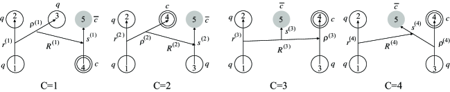
Figure 1: Four sets of the Jacobi coordinate systems. The light ($u,d$) quarks, labeled by particle $1-3$, are to be anti-symmetrized, while the particles 4 and 5 stand for $c$ and $\bar{c}$, respectively. Scatterings of $qqq+c\bar{c}$ and $qqc+q\bar{c}$ are described in the coordinates $C=1$ and 2, respectively.

The full wave function $\Psi_{JM}$ is written as a sum of components, each described in terms of one of the four Jacobi coordinate systems, namely

$$\Psi_{JM}=\sum_{C}{\cal A}_{123}\;\xi_{1}^{(C)}\eta_{T}^{(C)}\Big{[}\chi^{(C)}_{S(s\bar{s}\sigma)}\times\Big{[}\big{[}[\phi_{nl}^{(C)}({\boldsymbol{r}}^{(C)})\\ \varphi_{\nu\lambda}^{(C)}(\mbox{\boldmath$\rho$}^{(C)})]_{\Lambda}\psi_{NI}^{(C)}({\boldsymbol{R}}^{(C)})\big{]}_{I^{\prime}}\tilde{\psi}_{N^{\prime}K}^{(C)}({\boldsymbol{s}}^{(C)})\Big{]}_{L}\Big{]}_{J^{P}M}$$ (4)

where $C$ specifies the set of Jacobi coordinates and $\xi_{1}^{(c)}$, $\eta_{t}^{(c)}$ and $\chi^{(c)}_{S(s\bar{s}\sigma)}$ represent the color, isospin and spin wave functions, respectively. The orbital wave functions with appropriate orbital angular momenta are described by $\phi^{(C)}$, $\varphi^{(C)}$, $\psi^{(C)}$ and $\tilde{\psi}^{(C)}$. ${\cal A}_{123}$ denotes the anti-symmetrization operator for the light quarks (1,2,3). We consider the states with the total isospin $T=1/2$ and the total spin $S=1/2$ or 3/2. In the present analysis, we take the total orbital angular momentum $L=0$ only. Then the total spin-parity is either $J^{P}=1/2^{-}$ or $3/2^{-}$. According to the LHCb experiment, the observed pentaquark states may have $5/2^{-}$ or $3/2^{+}$. However, in the present calculation, the energies of the states with total angular momentum larger than 3/2 or with positive parity are located at much higher masses.

The color-singlet wave function, $\xi_{1}^{(C)}$, for each Jacobi configuration is chosen as

$$\begin{split}\xi_{1}^{(1)}&=[(123)_{1}(45)_{1}]_{1}\,,\\ \xi_{1}^{(2)}&=[(124)_{1}(35)_{1}]_{1}\,,\\ \xi_{1}^{(3)}&=[(12)_{\bar{3}}(34)_{\bar{3}}]_{3}5]_{1}\,,\\ \xi_{1}^{(4)}&=[(12)_{\bar{3}}[(34)_{\bar{3}}5]_{3}]_{1}\,.\end{split}$$ (5)

The spin and isospin wave functions are given by

$$\eta_{T}^{(C)}=[\eta_{1/2}(i)\eta_{1/2}(j)]_{t}\eta_{1/2}(k)]_{T=1/2},$$ (6)

$$\begin{aligned} &\chi^{(1)}_{S(s\bar{s}\sigma)}(123,4,5)=[[(12)_{s}3]_{\sigma}(45)_{\bar{s}}]_{S},\\ &\chi^{(2)}_{S(s\bar{s}\sigma)}(123,4,5)=[[(12)_{s}4]_{\sigma}(35)_{\bar{s}}]_{S},\\ &\chi^{(3)}_{S(s\bar{s}\sigma)}(123,4,5)=[[(12)_{s}(34)_{\bar{s}}]_{\sigma}5]_{S},\\ &\chi^{(4)}_{S(s\bar{s}\sigma)}(123,4,5)=[(12)_{s}[(34)_{\bar{s}}]5]_{\sigma}]_{S}.\end{aligned}$$ (7)

The spatial wave functions for each channel $(C)$ are expanded by multi-range Gaussians multiplied by spherical harmonics as

$$\begin{split}&\phi_{nlm}({\boldsymbol{r}})=N_{nl}\,r^{l}\>e^{-(r/r_{n})^{2}}\>Y_{lm}({\hat{\boldsymbol{r}}})\;,\\ &\varphi_{\nu\lambda\mu}(\mbox{\boldmath$\rho$})=N_{\nu\lambda}\,\rho^{\lambda}\>e^{-(\rho/\rho_{\nu})^{2}}\>Y_{\lambda\mu}({\hat{\mbox{\boldmath$\rho$}}})\;,\\ &\psi_{NIM}({\boldsymbol{R}})=N_{NI}\,R^{I}\>e^{-(R/R_{N})^{2}}\>Y_{IM}({\hat{\boldsymbol{R}}})\;,\\ &\psi_{N^{\prime}KM_{K}}({\boldsymbol{s}})=N_{N^{\prime}K}\,s^{K}\>e^{-(s/s_{N^{\prime}})^{2}}\>Y_{KM_{K}}({\hat{\boldsymbol{s}}})\;.\end{split}$$ (8)

Here, it is important to choose the Gaussian ranges to lie in geometric progression so that the basis functions are suitable for the descriptions of both short-range correlations and long-range asymptotic behavior without introducing too many free parameters (see, for example, Refs. Kamimura1988 ; Kame89 ; Hiyama2003 ; Hiya12FEW ; Hiya12PTEP ; Hiya12COLD ; Ohtsubo2013 ):

$$r_{n}=r_{1}\,a^{n-1}\;\quad\quad\> (n=1\ldots n_{\rm max})\;,$$ (9)

$$\rho_{\nu}=\rho_{1}\,b^{\nu-1}\; (\nu=1\ldots\nu_{\rm max})\;,$$

$$R_{N}=R_{1}\,A^{N-1}\; (N=1\ldots N_{\rm max})\;,$$

$$s_{N^{\prime}}=s_{1}\,A^{\prime N^{\prime}-1}\; (N^{\prime}=1\ldots N^{\prime}_{\rm max})\;.$$

In Eqs. (8) and (9), the channel index $(C)$ is omitted for simplicity, for example, $\boldsymbol{r^{(c)}}$ is replaced by $\boldsymbol{r}$. The dimension of the basis of Gaussian wave functions, $n_{\rm max}$, $\nu_{\rm max}$, $N^{\prime}_{\rm max}$ for $C=1$ to $4$ channels and $N_{\rm max}$ for $C=3$ and 4 channels is 5 or 6. And there are $N_{\rm max}=10$ Gaussian basis functions for $C=1$ and 2. Since these are scattering channels, it is necessary to have many basis functions. Thus in diagonalizing the five-body Hamiltonian for $J^{P}=1/2^{-}$ and $3/2^{-}$ states, we use about 40,000 basis functions, resulting in the same number of eigenstates for each $J^{P}$.

It should be noted here that all the obtained eigenvalues are discrete, as the wave function for ${\boldsymbol{R}}^{(C=1,2)}$ is expanded on a finite basis of functions localized within $R\lesssim 2\,R_{N}$. Namely, even the continuum states corresponding to the baryon-meson scattering solutions come out as discrete states. Therefore when we look for a compact pentaquark state, appearing as a sharp resonance embedded in the continuum, we need a method to distinguish the genuine resonances from the discretized scattering states. Here we adopt the real-scaling (stabilization) method, often used for analyzing electron-atom and electron-molecule scattering real-scal , and already introduced in a previous quark-model calculation Hiyama:2005cf . In the present case, as we have explained in the definition of the Jacobi coordinate systems, the continuum spectrum arises only from the factors of the wave functions that depend on ${\boldsymbol{R}}^{(1)}$ or ${\boldsymbol{R}}^{(2)}$. The factors of wave functions that depend on the coordinates other than ${\boldsymbol{R}}^{(1)}$ and ${\boldsymbol{R}}^{(2)}$ cannot have asymptotic states due to their colored configurations. We therefore scale the basis functions for the expansion of the wave functions along ${\boldsymbol{R}}^{(1)}$ and ${\boldsymbol{R}}^{(2)}$. To do this, we multiply all the range parameters simultaneously by a factor as $R_{N}\to\alpha R_{N}$. Then any continuum state will fall off towards its threshold, while a compact resonance state should stay as it is not affected by the boundary at a large distance.

III Results

Let us start with the calculation without the contributions from “continuum” (scattering) states. This corresponds to a conventional estimate in the quark model without coupling to fall-apart decaying channels. In our scheme, this can be done by including only the connected Jacobi coordinate systems, $C=3$ and 4 of Fig. 1. Solving the five-body Schrödinger equation for spin-parity $J^{P}=1/2^{-}$ and $3/2^{-}$ states, we obtain the masses shown in Fig. 2. We find that all the eigenvalues are found above the lowest meson-baryon threshold, $\eta_{c}N$ or ${J/\psi}N$. Nevertheless, as our wave function contains only the $C=3$ and 4 components, all the obtained states appear as “bound states” without the contribution from scattering states.

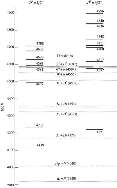
Figure 2: The calculated energy spectra for $J=1/2^{-}$ and $3/2^{-}$ states using the connected configurations of $C=3$ and 4. The dashed lines are thresholds

For the spin-parity $J^{P}=1/2^{-}$, the lowest state appears at 4119 MeV, which is above the hidden charm threshold, $\eta_{c}N$ and ${J/\psi}N$, and below the open charm one of $\Lambda_{c}D$. This result is compatible with, e.g., Ref. Richard:2017una , which uses the potential AL1. The second and third states appear at 4236 MeV and 4497 MeV, respectively. These states lie around the LHCb pentaquarks (4380 MeV and 4450 MeV) though their spin-parity assignments are different from those of the preferred ones ($3/2^{-}$ and $5/2^{+}$ respectively). In addition, we find several states around and above 4500 MeV. For $J=3/2^{-}$, the lowest state appears at 4221 MeV, whose energy is higher than the lowest $J^{P}=1/2^{-}$ state by about 100 MeV. It is, again compatible with Ref. Richard:2017una . It is followed by the second state at 4577 MeV, which is a region of several open channel thresholds.

For complete analysis, we need to include the scattering configurations such as $qqq+c\bar{c}$ and $qqc+q\bar{c}$. This can be achieved by including the $C=1$ and 2 configurations in our formulation. Now, the coupling of the scattering states may cause some (in fact many) of the “bound states” to disappear, melting away into the continuum spectrum. This was already pointed out for the $\Theta^{+}$ pentaquark Hiyama:2005cf . In the present case, the number of thresholds is significantly larger than that for the $\Theta^{+}$ system, and therefore the effects of the coupling is more pronounced. For instance, we have nine thresholds opening within 700 MeV from the lowest threshold in $J=1/2^{-}$ configurations, as indicated by the dashed lines in Fig. 2.

In order to investigate the nature of the bound states shown in Fig. 2 and their fate due to the coupling to scattering states, we investigate the behavior of the connected states coupled by a scattering state one by one in the real scaling method. Namely, we scale the range parameter $R_{N}$ of the Gaussian basis (see in (8)) as $R_{N}\to\alpha R_{N}$ for the Jacobi coordinates of $C=1$ or 2 i.e., $R_{N}=R_{N}^{(1)}$ and $R_{N}^{(2)}$. The eigenvalues corresponding to scattering states will fall down towards the threshold of the scattering state as the scaling factor $\alpha$ increases. On the other hand, resonance states will stay at a resonance energy independently from the scaling parameter $\alpha$.

To illustrate our method, let us study the two “connected” states, the one at 4119 MeV with $1/2^{-}$ and the one at 4236 MeV with $3/2^{-}$. We see that there are two open thresholds, ${J/\psi}N$ and $\eta_{c}N$ below the state at 4119 MeV, as shown in Fig. 2. We have performed calculations for the following two cases, (a) $C=3$ and 4 (connected configurations) with only $\eta_{c}N$ and (b) $C=3$ and 4 (connected configurations) with only ${J/\psi}N$. The coupling of the $\eta_{c}N$ or ${J/\psi}N$ corresponds to the inclusion of $c=1$ of Fig. 1 as it contains a configuration of $qqq$ and $c\bar{c}$ linked by $R_{1}$. The results are shown in Fig. 3(a) and 3(b), respectively, where we demonstrate discrete eigenenergies as functions of $\alpha$. There are about 30,000 basis functions, and thus about 30,000 eigenstates as discrete states. For the real scaling method, we scale the coordinate $R^{(1)}$ for $C=1$ configuration by a scaling factor $1.0<\alpha<1.5$

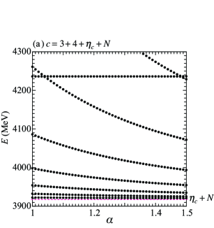
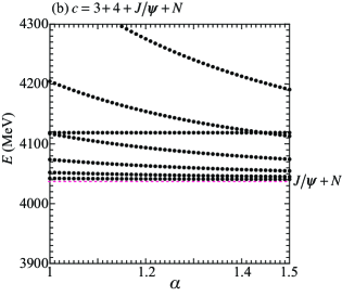
Figure 3: (color online) The stabilization plots of the eigenenergies $E$ of the psuedostates for $J=1/2^{-}$ with the respect to the scaling factor $\alpha$ in the case of (a) only connected configuration of $C=3+4$, and $\eta_{c}+N$ configuration, and of (b) only connected configurations of $C=3+4$ and ${J/\psi}+N$.

As seen in Fig. 3(a), we cannot find stable states around 4119 MeV: all eigenstates around this mass move towards the $\eta_{c}N$ threshold when $\alpha$ increases. This implies that the connected state at 4119 MeV strongly couples to $\eta_{c}N$ and melts away into the scattering state in the complete five-body calculation.

On the other hand, the connected state at 4236 MeV stays stable. A level repulsion (avoided crossing) is seen at $\alpha=1.04$ and $\alpha=1.48$. In the method of real scaling, the distance between the two levels at the repulsion point is related to the decay width. In the present case, the distances are small, which indicates that the state is a very sharp resonance where the connected state at 4236 MeV couples only weakly with $\eta_{c}N$.

To know the nature of the two connected states better, let us see Fig. 3(b) which shows the result of the calculation with $C=3+4+J/\psi N$ configurations. Now we see the opposite situation from Fig. 3(a). Namely, the connected state at 4119 MeV stays stable, while the one at 4236 MeV disappears.

From these observations, we may interpret that the state at 4119 MeV is dominated by $\eta_{c}$ and $N$ clusters, and the one at 4236 MeV by $J/\psi$ and $N$ clusters. These clusters interact only weakly and cannot hold bound nor resonant states. The appearance of the bound states in Fig. 2 is due to the inclusion of only the connected diagrams, $C=3$ and 4 of Fig. 1. We have seen that the two lowest connected states, the one at 4119 MeV and the one at 4236 MeV disappear in the full five-body calculation, and that we do not have any resonant state in the energy region from 3900 MeV to 4300 MeV.

We have repeated the same procedure to analyze each connected state given in Fig. 2 and summarized the results in Table 3 (a) for $J^{P}=1/2^{-}$ and in Table 3 (b) for $J^{P}=3/2^{-}$, where the results are shown for the dominant scattering configurations which couple to each connected state. Table II (a) shows that most of the $J=1/2^{-}$ connected states in the energy region from $E=4119$ MeV to $E=4673$ MeV have significant coupling to scattering states, and they do not survive as resonances. For instance, the state at 4497 MeV which is close to the observed $P_{c}$ couples strongly to $\eta_{c}N$, $\Lambda_{c}D^{*}$ and $\Sigma_{c}D$ configurations. In the present quark model Hamiltonian, there is not a sufficiently strong attractive force between these hadrons, and therefore, the bound states in the connected configurations do not survive as resonant states.

There are, however, exceptions; the states at 4708 MeV for $1/2^{-}$ and at 4896 MeV for $3/2^{-}$. They do not have any dominant cluster structure, and likely corresponds to a complicated five-quark configuration. To see this point better, we show the stabilization plots in Figs. 4 for the case of $1/2^{-}$. Figure 4(a) shows the result when only the scattering configurations $C=1$ and 2 are included, while (b) is for the full calculation. As expected there is not resonance structure there. However, by including the “seed” in connected configurations $C=3$ and 4, we find a resonance structure at around 4690 MeV as shown in Fig. 5, which is identified with the Feshbach resonance with its seed as the bound state at 4708 MeV in the connected configurations. The same analysis for $3/2^{-}$ indicates that the resonance appears at around 4920 MeV with the seed at 4896 MeV.

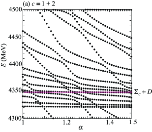
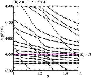
Figure 4: (color online) The stabilization plots of the eigenenergies $E$ of the pseudostates with the respect to the scaling factor $\alpha$ in the case of (a) only scattering configurations of $C=1$ and 2, and of (b) full configurations of $C=1$ to $4$. The Gaussian ranges $R_{N}$ for the coordinates ${\boldsymbol{R}_{1}}$ and ${\boldsymbol{R}_{2}}$ of $C=1$ and 2 configurations are scaled as $R_{N}\rightarrow\alpha R_{N}$ with $1.0$ to $1.5$.

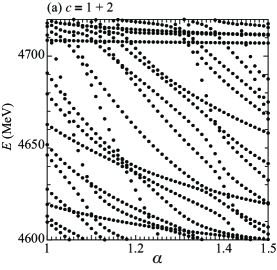
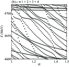
Figure 5: (color online) The stabilization plots of the eigenenergies $E$ of the pseudostates with the respect to the scaling factor $\alpha$ in the case of (a) only scattering configurations of $C=1$ and 2, and of (b) full configurations of $C=1$ to $4$. The Gaussian ranges $R_{N}$ for the coordinates ${\boldsymbol{R}_{1}}$ and ${\boldsymbol{R}_{2}}$ of $C=1$ and 2 configurations are scaled as $R_{N}\rightarrow\alpha R_{N}$ with $1.0$ to $1.5$.

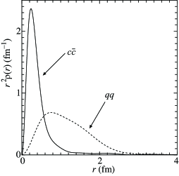
Figure 6: The calculated $qq$ and $c\bar{c}$ correlation function for $J=1/2^{-}$ state with full configurations. The solid line for $qq$ and the dashed line is for $c\bar{c}$.

Now let us see how the above results depend on the choice of the Hamiltonian. For this purpose, we have also used the AL1 potential in Ref. Semay:1994ht ; Silvestre . This potential also reproduces the ground states of the heavy mesons and baryons. We have found that the results of our five-body calculations are essentially not modified, but with small changes in resonance masses, 4690 MeV for $J=1/2^{-}$ and 4920 MeV for $J=3/2^{-}$.

Finally, we would like to study the structure of the resonant state found in the present work. We have calculated the two-body correlation function of $qq$ and of $c\bar{c}$ for the state at $E=4690$ MeV for $J^{P}=1/2^{-}$. The correlation functions are defined as

$$\begin{split}\rho_{qq}(r_{1})&=\int|\Psi_{JM}|^{2}d\boldsymbol{s}_{1}d\boldsymbol{R}_{1}d\mbox{\boldmath$\rho$}_{1}d\hat{\boldsymbol{r}}_{1}\\ \rho_{c\bar{c}}(s_{1})&=\int|\Psi_{JM}|^{2}d\boldsymbol{r}_{1}d\boldsymbol{R}_{1}d\mbox{\boldmath$\rho$}_{1}d\hat{\boldsymbol{s}}_{1}\,,\end{split}$$ (10)

where $\boldsymbol{r}_{1}$ and $\boldsymbol{s}_{1}$ are the relative distance between two light quarks $qq$ and $c\bar{c}$, as illustrated in Fig. 1, $C$ = 1. The integral was performed at $E=4689$ MeV with the scaling factor $\alpha=1.05$, A consistency was checked by integrating over either $\boldsymbol{r}_{1}$ or $\boldsymbol{s}_{1}$, where we have verified that integrated normalization is $0.9999$. Figure 6 shows the density distributions of $r^{2}\rho_{qq}$ and $r^{2}\rho_{c\bar{c}}$ as functions of the distance $r=\boldsymbol{r}_{1}=\boldsymbol{s}_{1}$. We find that quarks in the pentaquark resonance distribute only within a compact region. The peak positions indicate that the light quarks extend about 0.8 fm and the charmed quarks are restricted to about 0.2 fm, which is consistent with the sizes of the nucleon $N$ and the charmonia $J/\psi$ or $\eta_{c}$.

IV Summary

Motivated by the observation of pentaquark system of $P_{c}(4380)$ and $P_{c}(4450)$, we solved the five-body scattering problem for the $J^{P}=1/2^{-}$ and $3/2^{-}$ state.with Gaussian expansion supplemented by real scaling. Here we adopted non-relativistic quark model using AP1 potential proposed by Semay and Silvestre-Brac Semay:1994ht ; Silvestre . The potential reproduces the experimental ground state energies of heavy mesons and baryons entering the open-channel thresholds relevant for the $P_{c}$ system.

The main message is the clear possibility of distinguishing genuine resonances of the model from artifacts of the discretization. This opens new perspectives for quark model calculations in the multiquark sector.

In our calculation, based on a simple model of quark dynamics, two narrow states emerge, with a compact structure. They lie at 4690 MeV for $J=1/2^{-}$ and at 4920 MeV for $J=3/2^{-}$, too high in mass to be identified with any LHCb pentaquark. However, an improved quark model could probably lead to a better phenomenology. In particular, the model (1) is probed only for color singlet and antitriplet: the value of the potential in the sextet and octet color states can perhaps be modified, for instance by introducing three- or four-body forces.

We believe that our method, namely a Gaussian expansion of the wave function supplemented by real scaling, can be used to more sophisticated models applied to the hidden-charm pentaquarks and to other multiquark configurations.

Table 3: Dominant hadron-hadron component for the various bound states in Fig. 2 structure of each energy taking only connected configurations for (a)$J=1/2^{-}$ and $J=3/2^{-}$ states. Since the states at $E=4836$ and 4840 are close to each other, their hadron-hadron components have been merged. The states at $E=4708$ MeV and $E=4896$ MeV have no significant overlap with the open channels shown in Fig. 2.

(a) $J=1/2^{-}$	energy(MeV)	configuration
	$4119$	$\eta_{c}+N$
	$4236$	$J/\psi+N$, $\Lambda_{c}+D$
	$4497$	$\eta_{c}+N$,$\Lambda_{c}+D^{*}$, $\Sigma_{c}+D$
	$4581$	$J/\psi+N$
	$4593$	$\Lambda_{c}+D$
	$4629$	$\psi^{\prime}+N$
	$4679$	$\Sigma_{c}+D^{*}$
	$4708$	-
(b) $J=3/2^{-}$	energy(MeV)	configuration
	$4221$	$J/\psi+N$
	$4577$	$\Lambda_{c}+D^{*},\Sigma_{c}*D^{*},\Sigma_{c}^{*}+D^{*}$,$J/\psi+N$
	$4617$	$\Sigma_{c}^{*}+D$,$\Sigma_{c}^{*}+D^{*}$
	$4700$	$\Sigma_{c}^{*}+D$,$\Sigma_{c}^{*}+D^{*}$
	$4711$	$\Sigma_{c}+D^{*}$
	$4748$	$\Sigma_{c}^{*}+D$
	$4836$	$\Sigma_{c}^{*}+D^{*}$ or $\Sigma_{c}^{*}+D$
	$4840$	$\Sigma_{c}^{*}+D^{*}$ or $\Sigma_{c}^{*}+D$
	$4896$	-

- (1) S. K. Choi et al. [Belle Collaboration], Phys. Rev. Lett. 91, 262001 (2003) doi:10.1103/PhysRevLett.91.262001 [hep-ex/0309032].
- (2) R. Aaij et al. [LHCb Collaboration], Phys. Rev. Lett. 115, 072001 (2015) doi:10.1103/PhysRevLett.115.072001 [arXiv:1507.03414 [hep-ex]].
- (3) A. Hosaka, T. Iijima, K. Miyabayashi, Y. Sakai, and S. Yasui, Prog. Theor. Exp. Phys. 2016, 062C01 (2016) [arXiv:1603.09229 [hep-ph]].
- (4) H. X. Chen, W. Chen, X. Liu, and S. L. Zhu, Phys. Rept. 639, 1 (2016) [arXiv:1601.02092 [hep-ph]].
- (5) R. F. Lebed, R. E. Mitchell and E. S. Swanson, Prog. Part. Nucl. Phys. 93, 143 (2017) doi:10.1016/j.ppnp.2016.11.003 [arXiv:1610.04528 [hep-ph]].
- (6) M. Karliner, J. L. Rosner and T. Skwarnicki, arXiv:1711.10626 [hep-ph].
- (7) J. M. Richard, Few Body Syst. 57, no. 12, 1185 (2016) doi:10.1007/s00601-016-1159-0 [arXiv:1606.08593 [hep-ph]].
- (8) S. G. Yuan, K. W. Wei, J. He, H. S. Xu, and B. S. Zou, Eur. Phys. J. A 48, 61 (2012) [arXiv:1201.0807 [nucl-th]].
- (9) E. Santopinto and A. Giachino, Phys. Rev. D 96, 014014 (2017) [arXiv:1604.03769 [hep-ph]].
- (10) J. Wu, Y. R. Liu, K. Chen, X. Liu, and S. L. Zhu, Phys. Rev. D 95, 034002 (2017) [arXiv:1701.03873 [hep-ph]].
- (11) S. Takeuchi and M. Takizawa, Phys. Lett. B 764, 254 (2017) [arXiv:1608.05475 [hep-ph]].
- (12) L. Maiani, A. D. Polosa, and V. Riquer, Phys. Lett. B 749, 289 (2015) [arXiv:1507.04980 [hep-ph]].
- (13) G. N. Li, X. G. He, and M. He, JHEP 1512, 128 (2015) [arXiv:1507.08252 [hep-ph]].
- (14) A. Ali, I. Ahmed, M. J. Aslam, and A. Rehman, Phys. Rev. D 94, 054001 (2016) [arXiv:1607.00987 [hep-ph]].
- (15) R. F. Lebed, Phys. Lett. B 749, 454 (2015) [arXiv:1507.05867 [hep-ph]].
- (16) R. Zhu and C. F. Qiao, Phys. Lett. B 756, 259 (2016) [arXiv:1510.08693 [hep-ph]].
- (17) J. J. Wu, R. Molina, E. Oset, and B. S. Zou, Phys. Rev. Lett. 105, 232001 (2010) [arXiv:1007.0573 [nucl-th]].
- (18) J. J. Wu, R. Molina, E. Oset, and B. S. Zou, Phys. Rev. C 84, 015202 (2011) [arXiv:1011.2399 [nucl-th]].
- (19) C. Garcia-Recio, J. Nieves, O. Romanets, L. L. Salcedo, and L. Tolos, Phys. Rev. D 87, 074034 (2013) [arXiv:1302.6938 [hep-ph]].
- (20) M. Karliner and J. L. Rosner, Phys. Rev. Lett. 115, 122001 (2015) [arXiv:1506.06386 [hep-ph]].
- (21) R. Chen, X. Liu, X. Q. Li, and S. L. Zhu, Phys. Rev. Lett. 115, 132002 (2015) [arXiv:1507.03704 [hep-ph]].
- (22) L. Roca, J. Nieves, and E. Oset, Phys. Rev. D 92, 094003 (2015) [arXiv:1507.04249 [hep-ph]].
- (23) J. He, Phys. Lett. B 753, 547 (2016) [arXiv:1507.05200 [hep-ph]].
- (24) U. G. Meissner and J. A. Oller, Phys. Lett. B 751, 59 (2015) [arXiv:1507.07478 [hep-ph]].
- (25) H. X. Chen, W. Chen, X. Liu, T. G. Steele, and S. L. Zhu, Phys. Rev. Lett. 115, 172001 (2015) [arXiv:1507.03717 [hep-ph]].
- (26) T. Uchino, W. H. Liang, and E. Oset, Eur. Phys. J. A 52, 43 (2016) [arXiv:1504.05726 [hep-ph]].
- (27) Y. Shimizu, D. Suenaga, and M. Harada, Phys. Rev. D 93, 114003 (2016) [arXiv:1603.02376 [hep-ph]].
- (28) Y. Yamaguchi and E. Santopinto, Phys. Rev. D 96, 014018 (2017) [arXiv:1606.08330 [hep-ph]].
- (29) Y. Shimizu and M. Harada, [arXiv:1708.04743 [hep-ph]].
- (30) E. Hiyama, M. Kamimura, A. Hosaka, H. Toki and M. Yahiro, Phys. Lett. B 633, 237 (2006) doi:10.1016/j.physletb.2005.11.086 [hep-ph/0507105].
- (31) M. Kamimura, Phys. Rev. A38, 621 (1988).
- (32) E. Hiyama, Y. Kino and M. Kamimura, Prog. Part. Nucl. Phys. 51, 223 (2003).
- (33) E. Hiyama, B.F. Gibson and M. Kamimura, Phys. Rev. C 70 031001(R) (2004).
- (34) E. Hiyama and T. Yamada, Prog. Part. Nucl. Phys. 63, 339 (2009).
- (35) E. Hiyama, M. Kamimura, T. Motoba, T. Yamada, and Y. Yamamoto, Phys. Rev. Lett. 85, 270 (2000); E. Hiyama, M. Isaka, M. Kamimura, T. Myo and T. Motoba, Phys. Rev. C 91, 054316 (2015).
- (36) J. Mitroy, S. Bubin, W. Horiuchi, Y. Suzunki, L. Adamowicz, W. Cencek, K. Szalewicz, J. Komasa, D. Blume and K. Varga, Rev. Mod. Phys. 85 693 (2013).
- (37) C. Semay and B. Silvestre-Brac, Z. Phys. C 61, 271 (1994).
- (38) B. Silvestre-Brac, Few-body Syst. 20, 1 (1996).
- (39) H. Kameyama, M. Kamimura and Y. Fukushima, Phys. Rev. C 40, 974 (1989).
- (40) E. Hiyama, Few-Body Systems 53, 189 (2012).
- (41) E. Hiyama, Prog. Theor. Exp. Phys. 2012, 01A204 (2012).
- (42) E. Hiyama and M. Kamimura, Phys. Rev. A, 022502 85 (2012); ibid., 062505 85 (2012); ibid., 052514 90 (2014).
- (43) S. Ohtsubo, Y. Fukushima, M. Kamimura and E. Hiyama, Prog. Theor. Exp. Phys. 2013, 073D02 (2013).
- (44) J. Simon, J. Chem. Phys. 75, 2465 (1981).
- (45) J.-M. Richard, A. Valcarce and J. Vijande, Phys. Lett. B 774, 710 (2017) [arXiv:1710.08239 [hep-ph]].