Development of Singularities of the Skyrme Model

Abstract

The Skyrme model is a geometric field theory and a quasilinear modification of the Nonlinear Sigma Model (Wave Maps). In this paper we study the development of singularities for the equivariant Skyrme Model, in the strong-field limit, where the restoration of scale invariance allows us to look for self-similar blow-up behavior. After introducing the Skyrme Model and reviewing what’s known about formation of singularities in equivariant Wave Maps, we prove the existence of smooth self-similar solutions to the $5+1$-dimensional Skyrme Model in the strong-field limit, and use that to conclude that the solution to the corresponding Cauchy problem blows up in finite time, starting from a particular class of everywhere smooth initial data.

1 Background

One of the most extensively studied geometric field theories is Wave Maps. In this field theory, one studies a map from the $m+1$-dimensional Minkowski space, denoted by $\mathbb{R}^{1,m}$, with the usual Minkowski metric, denoted by $g$, to a complete $n$-dimensional Riemannian manifold $(\mathcal{N},h)$. A Wave Map, $U:\mathbb{R}^{1,m}\rightarrow\mathcal{N}$, is a critical point of the following action functional:

$$\mathcal{A}[U]=\frac{1}{2}\int tr_{g}\big{(}S(U)\big{)}\;d\mu_{g}$$ (1)

where $S(U):=U^{*}h$. The corresponding Euler-Lagrange Equation is the following nonlinear wave equation:

$$\Box_{g}U^{a}=-\Gamma^{a}_{bc}(U)\partial_{\mu}U^{b}\partial^{\mu}U^{c}$$ (2)

where $\Gamma^{a}_{bc}$ are the Christoffel symbols of the metric $h$. Much is known of this equation already. Of particular interest is its development of singularities in the equivariant case with $m=3$, $\mathcal{N}=S^{3}$, and $h$ the standard round metric established by Shatah (see [5]) and then generalized to rotationally symmetric, non-convex Riemannian manifolds by Shatah and Tahvildar-Zadeh (see [6] and [1]).

The Skyrme Model is a quasilinear adaptation of Wave Maps, originally proposed by physicist Tony Skyrme (see [8] and [7]) for applications to particle physics. Given $(\mathbb{R}^{1,m},g)$ and $(\mathcal{N},h)$ as above, a Skyrme Map, $U:\mathbb{R}^{1,m}\rightarrow\mathcal{N}$, is a critical point of the following functional:

$$\mathcal{S}[U]=\int\bigg{[}\frac{\alpha^{2}}{2}tr_{g}\big{(}S(U)\big{)}-\frac{\beta^{2}}{4}\Big{(}tr_{g}\big{(}S^{2}(U)\big{)}-tr_{g}^{2}\big{(}S(U)\big{)}\Big{)}\bigg{]}\;\;d\mu_{g}$$ (3)

for $\alpha,\beta\in\mathbb{R}$. In fact, the integrand of (3) is a combination of the first two symmetric polynomials of $S(U)$. One can immediately see that when $\beta=0$ and $\alpha=\pm 1$, we obtain (1). The corresponding Euler-Lagrange equation has been studied recently (see [3] and [2]). In particular, the Skyrme Model has been shown to posess large data global regularity in the equivariant case by Geba (see [3]) when $n=3$.

2 Main Problem and Main Result

We concern ourselves with the development of singularities of Skyrme Maps for the equivariant case of the Skyrme Model with $m=5$, $\mathcal{N}=S^{5}$, and $h$ the standard round metric in the strong-field limit. The solution to the equivariant, strong-field Skyrme Model equation of motion will be shown to blow up in finite time by the same mechanism as in [5].

The strong-field limit of the Skyrme Model is the limit of (3) when $\alpha\rightarrow 0$. Furthermore, an equivariant Skyrme Map, $U:\mathbb{R}^{1,5}\rightarrow S^{5}$, is a map of the form

$$U(t,r,\omega)=\big{(}u(t,r),\omega\big{)}$$ (4)

for some unknown $u:\mathbb{R}\times\mathbb{R}_{\geq 0}\rightarrow[0,\pi]$ where $t\in\mathbb{R}$ is the time coordinate, $r\in\mathbb{R}_{\geq 0}$ is the radial coordinate of $\mathbb{R}^{5}$, and $\omega\in S^{4}\subset\mathbb{R}^{5}$. Furthermore, under the strong-field limit and equivariant ansatz, the corresponding Euler-Lagrange equation for $u$ is the semilinear wave equation

$$u_{tt}-u_{rr}-\frac{2}{r}u_{r}+\cos u\bigg{(}\frac{u_{t}^{2}-u_{r}^{2}}{\sin u}+\frac{3\sin u}{r^{2}}\bigg{)}=0.$$ (5)

The following theorem is the main result of this paper:

Theorem 2.1.

Let $\alpha=0$ in (3). There exists a class of smooth initial data such that the corresponding Cauchy problem for the Euler-Lagrange equation of an equivariant Skyrme Map from $\mathbb{R}^{1,5}$ into $S^{5}$, in the strong field-limit, has a solution that blows up in finite time.

3 Summary of the Proof

Our goal is to construct smooth initial data for (5) which will develop a singularity in finite time. We will find such initial data by exploiting the scaling invariance of (5). That is, for any $\lambda\in\mathbb{R}-\{0\}$, (5) is invariant under the map $(t,r)\mapsto(\lambda t,\lambda r)$. Thus, we are motivated to find a self-similar solution $u(t,r)=w(-r/t)$ for some unknown $w:\mathbb{R}\to[0,\pi]$. For convenience, we define $\rho:=\dfrac{-r}{t}$. Such a nontrivial solution is constant along rays emanating from the origin of the Minkowski space and is thus multi-valued at the origin. This forces the derivative of $u$ to become unbounded and, consequently, a singularity develops.

Substituting $w$ into (5) results in the following ordinary differential equation

$$w_{\rho\rho}+\frac{2}{\rho}w_{\rho}-\bigg{[}\frac{3\sin^{2}w}{\rho^{2}(1-\rho^{2})}-w_{\rho}^{2}\bigg{]}\cot w=0.$$ (6)

We can modify (6) by setting $w=\cos^{-1}y$ for some unknown $y$, resulting in

$$y_{\rho\rho}+\dfrac{2}{\rho}y_{\rho}+\dfrac{3y\big{(}1-y^{2}\big{)}}{\rho^{2}\big{(}1-\rho^{2}\big{)}}=0.$$ (7)

If we can find a smooth solution to (7) for $\rho\in[0,1]$ satisfying the regularity conditions $y(0)=\pm 1$ and $y(1)=0$, then we can use that solution to specify smooth initial data in $B_{1}(0)\subset\Sigma_{-1}$ where $\Sigma_{-1}$ denotes the Cauchy hypersurface at $t=-1$. We can look in the past light cone of the origin of the Minkowski space in order to deduce that the derivative of the solution blows up at the origin.

First, we will show that an $H^{1}$ solution of (7) which is both continuous in $[0,1]$ and satisfies the regularity conditions is, in fact, a smooth solution of (7) . Then, we will set up a variational problem for which the critical points of some functional are solutions to (7). We will show that this functional achieves its minimum in the space for which it is defined and that this minimum has the necessary properties to be smooth as stated above.

4 Proof of Main Result

Remark 1.

We point out for notational convenience that by $B_{R}$, we mean $B_{R}(0)\subset\mathbb{R}^{3}$, the open ball of radius $R$ centered at the origin. Whenever we write $H^{1}$ or other function spaces, we always mean those functions on the ball $B_{1}$ unless stated otherwise. Furthermore, we will recycle the letter $C$ to denote a generic constant in our inequalities. Unless the explicit nature of this constant is important, $C$ may be a different constant in each instance.

Lemma 4.1.

Let $y\in H^{1}$ be a solution to (7) such that $y\in C[0,1]$, $y(0)=\pm 1$, and $y(1)=0$. Then $y\in C^{\infty}[0,1]$.

Proof.

The only values of $\rho$ for which a solution of (7) may not be smooth on the unit interval are $\rho=0$ and $\rho=1$. Since $y\in H^{1}$, then $y\in C^{0,\frac{1}{2}}(B_{1}\setminus B_{\alpha})$ for some fixed $\alpha\in(0,1)$ by Sobolev embedding. For $\rho\in(\alpha,1]$,

$$\begin{split}\big{|}y(1)-y(\rho)\big{|}&=\big{|}y(\rho)\big{|}\\ &<C\big{|}1-\rho\big{|}^{\frac{1}{2}}.\end{split}$$ (8)

Now, define $h_{y}(\rho):=\dfrac{-3y(\rho)\big{(}1-y^{2}(\rho)\big{)}}{\rho^{2}(1-\rho^{2})}$. Since $y\in C(\alpha,1]$,

$$\big{|}h_{y}(\rho)\big{|}\leq C_{\alpha}\dfrac{|y(\rho)|}{1-\rho}$$ (9)

for some constant $C_{\alpha}$ depending on $\alpha$. Consequently, for any $p\in\mathbb{N}$,

$$\begin{split}\int_{\alpha}^{1}|h_{y}|^{p}\;\rho^{2}d\rho&\leq C_{\alpha}\int_{\alpha}^{1}\frac{|y|^{p}}{|1-\rho|^{p}}d\rho\\ &\leq C_{\alpha}\Bigg{(}\int_{\alpha}^{1}\bigg{(}\frac{|y|}{1-\rho}\bigg{)}^{\frac{p}{p+1}}\;d\rho\Bigg{)}^{p+1}\Bigg{(}\int_{\alpha}^{1}1\;d\rho\Bigg{)}^{\frac{p}{p+1}}\\ &\leq C_{\alpha}(1-\alpha)^{\frac{p}{p+1}}\Bigg{(}\int_{\alpha}^{1}(1-\rho)^{\frac{-p}{2(p+1)}}\;d\rho\Bigg{)}^{p+1}\\ &<\infty.\end{split}$$ (10)

So, $h_{y}\in L^{p}(B_{1}\setminus B_{\alpha})$. Since (7) can be rewritten as $\Delta y=h_{y}$ and $h_{y}\in L^{p}(B_{1}\setminus B_{\alpha})$, we have that $y\in W^{2,p}(B_{1}\setminus B_{\alpha})$. Further, $y\in C^{k,\beta}(B_{1}\setminus B_{\alpha})$ for $k+\beta=p-\dfrac{3}{2}$ by Sobolev embedding. Thus, for any $k\in\mathbb{N}$, we can always find a $p$ which guarantees $y\in C^{k}(\alpha,1]$. Therefore, $y$ is a smooth function on the interval $(\alpha,1]$.

In order to show that $y$ is smooth at $\rho=0$, we change dependent variable. If $y(0)=1$, then we change to $z=y-1$. Similarly, if $y(0)=-1$, then we change to $z=y+1$. Each case is handled similarly with the appropriate change of sign. Without any loss of generality, we assume $y(0)=-1$ and change dependent variable to $z=y+1$. (7) becomes:

$$z_{\rho\rho}+\dfrac{2}{\rho}z_{\rho}-\dfrac{3z(z-1)\big{(}z-2\big{)}}{\rho^{2}\big{(}1-\rho^{2}\big{)}}=0$$ (11)

with $z(0)=0$ and $z(1)=1$. Furthermore, since $y\in C[0,1]$, we also have that $z\in C[0,1]$. We will show that the nonlinearity in (11) is integrable near $\rho=0$. Using this, we will show that the corresponding solution is smooth at $\rho=0$.

Multiplying (11) by $z$ and integrating from some $\varepsilon$ to $\delta$, $0<\varepsilon<\delta<1$ yields

$$\begin{split}&\int_{\varepsilon}^{\delta}zz_{\rho\rho}+\dfrac{2}{\rho}zz_{\rho}-\dfrac{3z^{2}(z-1)\big{(}z-2\big{)}}{\rho^{2}\big{(}1-\rho^{2}\big{)}}\;\;d\rho\\ &=\int_{\varepsilon}^{\delta}-z_{\rho}^{2}+\dfrac{2}{\rho}zz_{\rho}-\dfrac{3z^{2}(z-1)\big{(}z-2\big{)}}{\rho^{2}\big{(}1-\rho^{2}\big{)}}\;\;d\rho+\frac{1}{2}\partial_{\rho}(z^{2})\big{|}_{\varepsilon}^{\delta}\\ &=0.\end{split}$$ (12)

This implies

$$\begin{split}\int_{\varepsilon}^{\delta}z_{\rho}^{2}&-\dfrac{2}{\rho}zz_{\rho}+\dfrac{3z^{2}(z-1)\big{(}z-2\big{)}}{\rho^{2}\big{(}1-\rho^{2}\big{)}}\;\;d\rho=\frac{1}{2}\partial_{\rho}\big{(}z^{2}(\delta)\big{)}-\frac{1}{2}\partial_{\rho}\big{(}z^{2}(\varepsilon)\big{)}\\ &\leq\frac{1}{2}\partial_{\rho}\big{(}z^{2}(\delta)\big{)}\end{split}$$ (13)

since $z^{2}(0)=0$. So, (13) implies that we can take $\varepsilon\rightarrow 0$. For any $a<b$ and $a>0$,

$$z_{\rho}^{2}-\frac{2}{\rho}zz_{\rho}+\dfrac{3z^{2}(z-1)\big{(}z-2\big{)}}{\rho^{2}\big{(}1-\rho^{2}\big{)}}=\Big{(}1-\frac{a^{2}}{b^{2}}\Big{)}z_{\rho}^{2}+\Big{(}\frac{a}{b}z_{\rho}-\frac{b}{a}\frac{z}{\rho}\Big{)}^{2}+\Bigg{[}\frac{3z^{2}(z-1)\big{(}z-2\big{)}}{\rho^{2}\big{(}1-\rho^{2}\big{)}}-\frac{b^{2}}{a^{2}}\frac{z^{2}}{\rho^{2}}\Bigg{]}.$$ (14)

We can pick $\delta$ small enough so that $3z^{2}(z-1)\big{(}z-2\big{)}\approx 6z^{2}$ since $z$ is continuous on $[0,\delta)$. The third term in (14) becomes

$$\begin{split}&\frac{3z^{2}(z-1)\big{(}z-2\big{)}}{\rho^{2}\big{(}1-\rho^{2}\big{)}}-\frac{b^{2}}{a^{2}}\frac{z^{2}}{\rho^{2}}\approx\Big{(}\frac{6a^{2}-b^{2}(1-\delta^{2})}{a^{2}(1-\delta^{2})}\Big{)}\frac{z^{2}}{\rho^{2}}.\end{split}$$ (15)

Define the set

$$\mathbb{A}:=\Bigg{\{}(a,b)\in\mathbb{N}\times\mathbb{N}:0<a<b,\;\;\frac{6a^{2}-b^{2}(1-\delta^{2})}{a^{2}(1-\delta^{2})}>0\Bigg{\}}.$$ (16)

For any such $\delta$, it is possible to find a constant $C$ depending on $\delta$, such that

$$C(\delta)=\min_{(a,b)\in\mathbb{A}}\Bigg{\{}1-\frac{a^{2}}{b^{2}},\frac{6a^{2}-b^{2}(1-\delta^{2})}{a^{2}(1-\delta^{2})}\Bigg{\}}.$$ (17)

Then, we can bound the first and third terms of (14) from below by the following

$$\begin{split}z_{\rho}^{2}-\frac{2z_{\rho}z}{\rho}+\frac{3z^{2}(z-1)(z-2)}{\rho^{2}(1-\rho^{2})}&\geq\Big{(}1-\frac{a^{2}}{b^{2}}\Big{)}z_{\rho}^{2}+\Bigg{[}\frac{3z^{2}(z-1)\big{(}z-2\big{)}}{\rho^{2}\big{(}1-\rho^{2}\big{)}}-\frac{b^{2}}{a^{2}}\frac{z^{2}}{\rho^{2}}\Bigg{]}\\ &\geq C(\delta)\Big{(}z_{\rho}^{2}+\frac{z^{2}}{\rho^{2}}\Big{)}.\end{split}$$ (18)

This implies

$$\begin{split}&z_{\rho}^{2}+\frac{z^{2}}{\rho^{2}}\leq\frac{1}{C(\delta)}\Bigg{[}z_{\rho}^{2}-\frac{2z_{\rho}z}{\rho}+\frac{3z^{2}(z-1)\big{(}z-2\big{)}}{\rho^{2}\big{(}1-\rho^{2}\big{)}}\Bigg{]}.\end{split}$$ (19)

Further, (13) and (19) imply

$$\begin{split}\int_{0}^{\delta}z_{\rho}^{2}+\frac{z^{2}}{\rho^{2}}\;\;d\rho&\leq\frac{1}{C(\delta)}\int_{0}^{\delta}z_{\rho}^{2}-\frac{2z_{\rho}z}{\rho}+\frac{3z^{2}(z-1)\big{(}z-2\big{)}}{\rho^{2}\big{(}1-\rho^{2}\big{)}}\;\;d\rho\\ &\leq\frac{1}{2C(\delta)}\partial_{\rho}\big{(}z^{2}(\delta)\big{)}.\end{split}$$ (20)

Thus, for any $\delta>0$ we pick $\alpha=\dfrac{1}{2}\delta$. By taking $\delta>0$, we guarantee that (20) is finite. This implies that

$$\begin{split}z_{\rho\rho}+\frac{2}{\rho}z_{\rho}-\frac{6z}{\rho^{2}}&=\frac{3z(z-1)\big{(}z-2\big{)}}{\rho^{2}\big{(}1-\rho^{2}\big{)}}-\frac{6z}{\rho^{2}}\\ &=:\frac{f(z)}{\rho^{2}}\\ &\leq C\frac{z^{2}}{\rho^{2}}\end{split}$$ (21)

is integrable on $[0,\delta)$.

Now, we will show that $z$, the solution to (11), is smooth at $\rho=0$. Let $\rho=e^{t}$ for $t\in(-\infty,0]$. Then (21) becomes

$$z^{\prime\prime}+z^{\prime}-6z=f(z)$$ (22)

where the prime now denotes derivative with respect to $t$. The solutions to the homogeneous problem are $e^{-3t}$ and $e^{2t}$. Variation of parameters tells us that the solution to (22) is

$$z(t)=\lim_{a\rightarrow-\infty}\Bigg{[}e^{-3t}\Big{(}A(a)+\int_{a}^{t}f\big{(}z(s)\big{)}e^{3s}\;\;ds\Big{)}-e^{2t}\Big{(}B(a)+\int_{a}^{t}f\big{(}z(s)\big{)}e^{-2s}\;\;ds\Big{)}\Bigg{]}.$$ (23)

Introduce a new parameter $b<a$ in order to rewrite (23) as

$$z(t)=\lim_{a\rightarrow-\infty}\Bigg{[}e^{-3t}\Big{(}A(a)+\int_{a}^{b}f\big{(}z(s)\big{)}e^{3s}\;\;ds+\int_{b}^{t}f\big{(}z(s)\big{)}e^{3s}\;\;ds\Big{)}-e^{2t}\Big{(}B(a)+\int_{a}^{t}f\big{(}z(s)\big{)}e^{-2s}\;\;ds\Big{)}\Bigg{]}.$$ (24)

We look at the limit $b\rightarrow-\infty$ and then $t\rightarrow-\infty$. First, note that $\lim_{t\rightarrow-\infty}z(t)=0$ since $z$ is assumed to be continuous. Clearly,

$$e^{2t}\Big{(}B(a)+\int_{a}^{t}f\big{(}z(s)\big{)}e^{-2s}\;\;ds\Big{)}\rightarrow 0$$ (25)

as $t\rightarrow-\infty$. Also,

$$\begin{split}e^{-3t}\int_{b}^{t}\Big{|}f\big{(}z(s)\big{)}\Big{|}e^{3s}\;\;ds&\leq\int_{b}^{t}\Big{|}f\big{(}z(s)\big{)}\Big{|}\;\;ds\\ &\rightarrow 0\end{split}$$ (26)

as $b\rightarrow-\infty$ and $t\rightarrow-\infty$ since $f$ is a polynomial in $z$. Further,

$$\int_{a}^{b}f\big{(}z(s)\big{)}e^{3s}\;\;ds\rightarrow 0$$ (27)

as $b\rightarrow-\infty$. So, it must be the case that

$$e^{-3t}A(a)\rightarrow 0$$ (28)

as $t\rightarrow-\infty$ by the continuity of $z$. Since $A$ is independent of $t$, $A\equiv 0$. Now, examine the first derivative of $z$,

$$z^{\prime}(t)=-3e^{-3t}\int_{-\infty}^{t}f\big{(}z(s)\big{)}e^{3s}\;\;ds-2e^{2t}\lim_{a\rightarrow-\infty}\Bigg{(}B(a)+\int_{a}^{t}f\big{(}z(s)\big{)}e^{-2s}\;\;ds\Bigg{)}.$$ (29)

As $t\rightarrow-\infty$, the second term goes to $0$ due to (25). The first term goes to $0$ due to (26). So, $z^{\prime}(t)\rightarrow 0$ as $t\rightarrow-\infty$. This can only be the case if the solution is on the unstable manifold of (22), implying $|e^{-2t}z(t)|<1$ for sufficiently small $t$. Thus, in a small neighborhood around $0$, $|z(\rho)|\leq\rho^{2}$ implying that $z$ is $C^{1}[0,\delta)$ and consequently a smooth function of $\rho$ in that neighborhood. Combining this with the result from $(\alpha,1]$, we obtain that $y$ is a smooth function of $\rho\in[0,1]$. ∎

Next, we will find a solution to (7) which satisfies the hypotheses of Lemma 4.1. So, we will consider a variational problem with the functional

$$J[\psi]=\frac{1}{2}\int_{0}^{1}\Bigg{[}\psi_{\rho}^{2}-\frac{1}{\rho^{2}(1-\rho^{2})}3\psi^{2}\Big{(}1-\frac{1}{2}\psi^{2}\Big{)}\Bigg{]}\;\;\rho^{2}d\rho,$$ (30)

defined over the space

$$X:=\Big{\{}\psi\in H^{1}:\psi\;\text{radial},\;\psi(1)=0\Big{\}}.$$ (31)

It is a routine calculation to show that critical points of (30) satisfy (7). We choose to regularize $J$ by considering the functional

$$\begin{split}&J[\psi]=\frac{1}{2}\int_{0}^{1}\Bigg{[}\psi_{\rho}^{2}+\frac{1}{\rho^{2}(1-\rho^{2})}F(\psi)\Bigg{]}\;\;\rho^{2}d\rho,\\ &F(\psi)=\begin{cases}-3\psi^{2}\Big{(}1-\frac{1}{2}\psi^{2}\Big{)};&|\psi|<1\\ \varphi(\psi);&\text{otherwise}\\ 0;&|\psi|\geq\sqrt{2}\end{cases}\end{split}$$ (32)

where $\varphi(\psi)$ is a smooth function of $\rho\in[0,1]$ for any $\psi\in X$ such that $\varphi$ increases(decreases) monotonically to(from) $-3\psi^{2}\Big{(}1-\frac{1}{2}\psi^{2}\Big{)}$ from(to) $0$ for values of $\rho$ in which $1\leq|\psi(\rho)|\leq\sqrt{2}$. Along the way, we will show that our result is independent of the regularization we made.

Lemma 4.2.

$J$ is a $C^{1}$ functional on $X$ that is bounded from below. In particular, $J$ and its first derivative are Lipschitz continuous on $X$.

Proof.

For any $u,v\in X$,

$$\begin{split}\frac{1}{2}\Bigg{|}\int_{0}^{1}\frac{3}{\rho^{2}(1-\rho^{2})}\bigg{[}u^{2}\Big{(}1-\frac{1}{2}u^{2}\Big{)}-v^{2}\Big{(}1&-\frac{1}{2}v^{2}\Big{)}\bigg{]}\;\;\rho^{2}d\rho\Bigg{|}\leq C\int_{0}^{1}\frac{|u-v|}{\rho^{2}(1-\rho)}\bigg{|}(u+v)\Big{(}1-\frac{1}{2}(u^{2}+v^{2})\Big{)}\bigg{|}\;\;\rho^{2}d\rho\\ &\leq C\int_{0}^{1}\frac{|u-v|}{\rho^{2}(1-\rho)}\;\;\rho^{2}d\rho.\end{split}$$ (33)

Integrating from $0$ to $\beta$ with $\beta\in(0,1)$,

$$\begin{split}\int_{0}^{\beta}\frac{|u-v|}{\rho^{2}(1-\rho)}\;\;\rho^{2}d\rho&\leq C\Bigg{(}\int_{0}^{\beta}|u-v|^{6}\;\;\rho^{2}d\rho\Bigg{)}^{1/6}\Bigg{(}\int_{0}^{\beta}\rho^{-5/2}d\rho\Bigg{)}^{5/6}\\ &\leq C\|u_{\rho}-v_{\rho}\|_{L^{2}}\end{split}$$ (34)

and from $\beta$ to $1$

$$\begin{split}\int_{\beta}^{1}\frac{|u-v|}{\rho^{2}(1-\rho)}\;\;\rho^{2}d\rho&\leq C\Bigg{(}\int_{\beta}^{1}|u-v|^{6}\;\;\rho^{2}d\rho\Bigg{)}^{1/9}\Bigg{(}\int_{\beta}^{1}\frac{|u-v|^{3/8}}{(1-\rho)^{9/8}}\;\;d\rho\Bigg{)}^{8/9}\\ &\leq C\|u_{\rho}-v_{\rho}\|_{L^{2}}\Bigg{(}\int_{\beta}^{1}\frac{d\rho}{(1-\rho)^{15/16}}\Bigg{)}^{8/9}\\ &\leq C\|u_{\rho}-v_{\rho}\|_{L^{2}}.\end{split}$$ (35)

This implies

$$\begin{split}\Big{|}J[u]-J[v]\Big{|}&<C\|u_{\rho}-v_{\rho}\|_{L^{2}}\\ &\leq C\|u_{\rho}-v_{\rho}\|_{H^{1}}.\end{split}$$ (36)

Thus, $J$ is Lipschitz continuous on $X$. Further,

$$\int_{0}^{1}\Bigg{|}\frac{u(1-u^{2})-v(1-v^{2})}{\rho^{2}(1-\rho^{2})}\Bigg{|}\;\;\rho^{2}d\rho\leq C\int_{0}^{1}\frac{|u-v|}{\rho^{2}(1-\rho)}\;\;\rho^{2}d\rho.$$ (37)

So, (34) and (35) imply that $J$ is $C^{1}$ on $X$ and, more specifically, $J^{\prime}$ is Lipschitz continuous on $X$.

Now, compute (36) with $v\equiv 0$. The following holds:

$$\begin{split}J[u]&=C\|u_{\rho}\|_{L^{2}}^{2}-\frac{1}{2}\int_{0}^{1}\frac{3}{\rho^{2}(1-\rho^{2})}u^{2}\Big{(}1-\frac{1}{2}u^{2}\Big{)}\;\;\rho^{2}d\rho\\ &\geq C\big{(}\|u_{\rho}\|_{L^{2}}^{2}-\|u_{\rho}\|_{L^{2}}\big{)}.\end{split}$$ (38)

Thus, $J$ is bounded from below. ∎

Lemma 4.3.

If $y\in X$ is a minimizer of $J$, then $y(0)\neq 0$.

Proof.

Since $y\in X$ is a minimizer of (32), it satisfies the Euler-Lagrange equation (7). We can convert (7) to the three-dimensional, autonomous smooth dynamical system:

$$\begin{bmatrix}\dot{y}\\ \dot{q}\\ \dot{\rho}\end{bmatrix}=\begin{bmatrix}\big{(}1-\rho^{2}\big{)}q\\ \big{(}\rho^{2}-1\big{)}q-3y\big{(}1-y^{2}\big{)}\\ \rho\big{(}1-\rho^{2}\big{)}\end{bmatrix}=:\dot{Y}(y,q,\rho)$$ (39)

where $q=\rho y_{\rho}$ and the dot represents derivative with respect to the independent variable found by solving $\dot{\rho}=\rho(1-\rho^{2})$. This smooth dynamical system has equilibrium points:

$$(y,q,\rho)\in\big{\{}(0,0,0),(\pm 1,0,0),(\pm 1,\tilde{q},1),(0,\tilde{q},1):\tilde{q}\in\mathbb{R}\big{\}}.$$ (40)

Our goal is to exclude any solution with $y(0)=0$. We do this by showing that the only solution with $y(0)=0$ is the constant solution $y_{*}\equiv 0$. The eigenvalues of $D\dot{Y}(0,0,0)$ are

$$\Big{\{}\dfrac{1}{2}(-1+i\sqrt{11}),\dfrac{1}{2}(-1-i\sqrt{11}),1\Big{\}}$$ (41)

with corresponding eigenvectors

$$\Bigg{\{}\begin{bmatrix}\dfrac{1}{6}(-1-i\sqrt{11})\\ 1\\ 0\end{bmatrix},\begin{bmatrix}\dfrac{1}{6}(-1+i\sqrt{11})\\ 1\\ 0\end{bmatrix},\begin{bmatrix}0\\ 0\\ 1\end{bmatrix}\Bigg{\}}.$$ (42)

Thus, the unstable manifold of the equilibrium point $(0,0,0)$ is the line defined by $(0,0,\rho)$ for $\rho\in[0,1]$. By the uniqueness of solutions to autonomous dynamical systems, we know that $y=y_{*}$ is, in fact, the only solution with $y(0)=0$. For if it were not, then any other solution, namely $z$, will have an orbit tangent to $y_{*}$ only at $\rho=0$. In order for $z$ to not equal $y_{*}$, the orbit of $z$ must diverge from that of $y_{*}$. But this cannot be the case since the unstable manifold at $(0,0,0)$ is one-dimensional.

Now, any solution of (7) satisfies $y(0)=\pm 1$ or is $y_{*}\equiv 0$. We rule out $y_{*}$ by showing that it is not a minimizer of $J$. First, we notice that $J[y_{*}]\equiv 0$. We can construct a variation of $y_{*}$ with a smaller value of $J$ by examining the second derivative of $J$ at any $\bar{y}\in X$, $\eta\in C_{0}^{\infty}(B_{1})$:

$$\frac{d^{2}}{d\varepsilon^{2}}J[\bar{y}+\varepsilon\eta]\Big{|}_{\varepsilon=0}=\int_{0}^{1}\eta_{\rho}^{2}\;\;\rho^{2}d\rho-6\int_{0}^{1}(1-3\bar{y}^{2})\frac{\eta^{2}}{\rho^{2}(1-\rho^{2})}\;\;\rho^{2}d\rho.$$ (43)

Taking $\bar{y}=y_{*}$, we get

$$\frac{d^{2}}{d\varepsilon^{2}}J[y_{*}+\varepsilon\eta]\Big{|}_{\varepsilon=0}=\int_{0}^{1}\eta_{\rho}^{2}\;\;\rho^{2}d\rho-6\int_{0}^{1}\frac{\eta^{2}}{\rho^{2}(1-\rho^{2})}\;\;\rho^{2}d\rho.$$ (44)

In [6], it is shown that there is an $\bar{\eta}\in C_{0}^{\infty}(B_{1})$ such that

$$\int_{0}^{1}\bar{\eta}_{\rho}^{2}\;\;\rho^{2}d\rho<6\int_{0}^{1}\frac{\bar{\eta}^{2}}{\rho^{2}(1-\rho^{2})}\;\;\rho^{2}d\rho.$$ (45)

Thus,

$$\frac{d^{2}}{d\varepsilon^{2}}J[y_{*}+\varepsilon\bar{\eta}]\Big{|}_{\varepsilon=0}<0.$$ (46)

This implies that $J[y_{*}+\varepsilon\bar{\eta}]<J[y_{*}]$. Since $y_{*}+\varepsilon\bar{\eta}\in X$, $y_{*}$ cannot be a minimizer of $J$. Therefore, no minimizer of $J$ will satisfy $y(0)=0$ and, subsequently, it must be the case that $y(0)=\pm 1$. ∎

Remark 2.

Lemma 4.3 also proves that a minimizer $y$ of $J$, if it exists, satisifies $J[y]<0$.

Lemma 4.4.

Let $y\in X$ be a minimizer of $J$ with $y(0)=\pm 1$ and $y(1)=0$. Then $y$ is monotone.

Proof.

Assume that $y$ is not a monotone function. We will show that $y$ is not a minimizer, contradicting the hypotheses of Lemma 4.4. Without any loss of generality, we can assume $y(0)=-1$ since anything we show for the other case can be done in the same way. There are two cases to consider:

1. $y$ does not exceed $0$ but decreases on some interval and then increases to $0$ (depicted in Figure 1), and

   

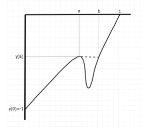
   Figure 1: Example of case 1. The bold dashed line represents the construction of (47).

2. $y$ exceeds $0$ and eventually decreases to $0$ at $\rho=1$ (depicted in Figures 2 and 3).

   

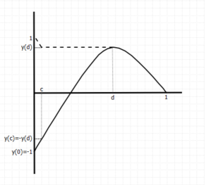
   Figure 2: Example of case 2, sub-case 1. The bold dashed line represents the construction of (48).

   

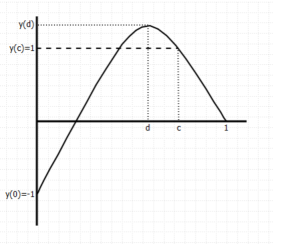
   Figure 3: Example of case 2, sub-case 2. The bold dashed line represents the construction of (49).

In the first case, there exists an interval $[a,b]$, $0\leq a<b\leq 1$, in which $y(a)=y(b)<0$ but $y(a)>y(\rho)$ for $\rho\in(a,b)$. Consider the function

$$\tilde{y}(\rho)=\begin{cases}y(\rho)&\rho\in[0,a)\bigcup(b,1]\\ y(a)&\rho\in[a,b].\end{cases}$$ (47)

Since $F[y(a)]<F[y(\rho)]$ for $\rho\in[a,b]$, $J[\tilde{y}]<J[y]$. Thus, we have constructed a new function with a smaller value of $J$.

In the second case, there exists an interval $[a,b]$, $0<a<b\leq 1$ in which $y(a)=y(b)=0$ but $y(\rho)>0$ for $\rho\in(a,b)$. Further, there exists $d\in(a,b)$ such that $y(\rho)\leq y(d)$ for all $\rho\in[a,b]$. There are now two sub-cases to consider: $y(d)<1$ and $y(d)\geq 1$.

If $y(d)<1$, then there must be some $c<d$ such that $y(c)=-y(d)$. We want to reflect the portion of the graph of $y$ before $c$ and then repeat the process used in the first case. This is done by considering the function

$$\tilde{y}(\rho)=\begin{cases}-y(\rho)&\rho\in[0,c)\\ y(d)&\rho\in[c,d]\\ y(\rho)&\rho\in(d,1].\end{cases}$$ (48)

Since $F[y(d)]<F[y(\rho)]$ for $\rho\in[c,d]$, $J[\tilde{y}]<J[y]$.

If $y(d)\geq 1$, then there must be some $c>d$ such that $y(c)=1$. We then consider the function

$$\tilde{y}(\rho)=\begin{cases}1&\rho\in[0,c]\\ y(\rho)&\rho\in(c,1].\end{cases}$$ (49)

Since $F[1]<F[y(\rho)]$ for $\rho\in[0,c]$, $J[\tilde{y}]<J[y]$.

In each case, we have shown that a non-monotone minimizer of $J$ with $y(0)=\pm 1$ and $y(1)=0$ is not actually a minimizer of $J$. Therefore, a minimizer of $J$, $y\in X$, with $y(0)=\pm 1$ and $y(1)=0$ is a monotone function. ∎

Lemma 4.5.

$J$ attains its minimum in $X$ at a smooth function $y$ such that $-1\leq y\leq 1$.

Proof.

We employ an argument similar to that of the proof of the existence of a minimizer for an energy functional used in [4], page 276. Let $\{y_{n}\}$ be a minimizing sequence of $J$. That is, $\lim_{n\rightarrow\infty}J[y_{n}]=\inf_{\psi\in X}J[\psi]:=J_{0}$. By (38), $\{y_{n}\}$ is a bounded sequence in $H^{1}$. The Banach-Alaglou Theorem implies that there is a subsequence, also denoted $\{y_{n}\}$ which is weakly convergent in $H^{1}$ and strongly convergent in $L^{2}$ to a function $y\in X$. Furthermore, there exists a constant $C$ such that

$$\frac{y_{n}^{2}\Big{(}1-\frac{1}{2}y_{n}^{2}\Big{)}}{\rho^{2}(1-\rho^{2})}\leq C\Big{(}1+\frac{1}{\rho^{2}}\Big{)}$$ (50)

for all $n$. This is certainly integrable on $B_{1}$. Even further, $y_{n}^{2}\Big{(}1-\frac{1}{2}y_{n}^{2}\Big{)}\rightarrow y^{2}\Big{(}1-\frac{1}{2}y^{2}\Big{)}$ almost everywhere. By the Dominated Convergence Theorem and weak lower semicontinuity of the $H^{1}$ norm,

$$\begin{split}J[y]&=J\big{[}\lim_{n\rightarrow\infty}y_{n}\big{]}\\ &\leq\lim_{n\rightarrow\infty}J[y_{n}]\\ &=:J_{0}.\end{split}$$ (51)

Since $J_{0}$ is the infimum of $J$, (51) implies $J[y]=J_{0}$. Consequently, the convergence is strong in $H^{1}$. Therefore, $J$ attains its minimum at a function $y\in X$. Further, $y$ is continuous since the $\alpha$-limit set of the corresponding smooth dynamical system in Lemma 4.3 tells us $y(0)=\pm 1$. By Lemma 4.4, $y$ is also monotone. Thus, $|y|\leq 1$. Therefore, by Lemma 4.1, $y$ is a smooth function of $\rho\in[0,1]$. ∎

Remark 3.

Since the solution satisfies $|y|\leq 1$, our minimization problem is independent of the regularization we placed on (30). Thus, Lemmas 4.1-4.5 are true for (30) as well as (32).

Now we can state the proof of Theorem 2.1:

Proof.

As previously stated, the Euler-Lagrange equation of the strong-field, equivariant Skyrme Map $U(t,r,\omega)=\big{(}u(t,r),\omega\big{)}$ is given by

$$u_{tt}-u_{rr}-\frac{2}{r}u_{r}+\cos u\bigg{(}\frac{u_{t}^{2}-u_{r}^{2}}{\sin u}+\frac{3\sin u}{r^{2}}\bigg{)}=0.$$ (52)

Let $\phi(x)$, $x=(r,\omega)\in\mathbb{R}^{5}$ and $\omega\in S^{4}\subset\mathbb{R}^{5}$, be the smooth function defined by

$$\phi(x)=(\cos^{-1}y(r),\omega)$$ (53)

where $y$ is a smooth solution to (7) with $y(0)=\pm 1$ and $y(1)=0$. We can supply the following Cauchy data to (52):

$$\begin{split}&U(-1,x)=\phi(x)\\ \partial_{t}&U(-1,x)=x^{i}\partial_{i}\phi\end{split}$$ (54)

Here, it is implicitly understood that the equations for the angles, $\omega$, is trivial. Then in the past light cone of the origin of the Minkowski space, the solution is

$$U(t,x)=\phi(-x/t).$$ (55)

Since the solution is multivalued at the origin, $\partial_{i}U(t,0)\rightarrow\infty$ as $t\rightarrow 0$. ∎

This concludes the argument and shows that there is a class of smooth initial data for the equivariant, strong-field Skyrme Model equation of motion which develops a singularity in finite time.

References

[1]
T. Cazenave, J. Shatah, and A. S. Tahvildar-zadeh.
Harmonic maps of the hyperbolic space and development of
singularities in wave maps and yang-mills fields.
Annales de l’Institut Henri Poincaré Physique Théorique,
68, 1998.
[2]
D.-A. Geba and D. da Silva.
On the regularity of the dimensional equivariant skyrme model.
Proceedings of the American Mathematical Society,
141(6):2105–2115, 2013.
[3]
D.-A. Geba and M. G. Grillakis.
Large data global regularity for the classical equivariant skyrme
model.
2017.
[4]
E. H. Lieb and M. Loss.
Analysis.
American Mathematical Society, 1997.
[5]
J. Shatah.
Weak solutions and development of singularities of the
-model.
Communications on Pure and Applied Mathematics, 41(4):459–469,
1988.
[6]
J. Shatah and A. S. Tahvildar-Zadeh.
On the cauchy problem for equivariant wave maps.
Communications on Pure and Applied Mathematics, 47(5):719–754,
1994.
[7]
T.H.R. Skyrme.
A non-linear field theory.
Proc. R. Soc. London, 260, 1961.
[8]
T.H.R. Skyrme.
A unified field theory of mesons and baryons.
Nuclear Physics, 31, 1962.