Universal behavior of the full particle statistics of one-dimensional Coulomb gases with an arbitrary external potential

Abstract

We present a complete theory for the full particle statistics of the positions of bulk and extremal particles in a one-dimensional Coulomb Gas (CG) with an arbitrary potential, in the typical and large deviations regimes. Typical fluctuations are described by a universal function which depends solely on general properties of the external potential. The rate function controlling large deviations is, rather unexpectedly, not strictly convex and has a discontinuous third derivative around its minimum for both extremal and bulk particles. This implies, in turn, that the rate function cannot predict the anomalous scaling of the typical fluctuations with the system size. Moreover, its asymptotic behavior for extremal particles differs from the predictions of the Tracy-Widom distribution. Thus many of the paradigmatic properties of the full particle statistics of two-dimensional systems do not carry out into their one-dimensional counterparts, hence proving that 1d CG belongs to a different universality class. Our analytical expressions are thoroughly compared with Monte Carlo simulations showing excellent agreement.

Being universality one of the pillars of modern theoretical physics, an important goal is to understand under which conditions universal properties do emerge in strongly correlated systems, together with their range of validity. Pursuing an answer to this poignant question, classical ensembles of random matrices have become a mathematical laboratory that allows to test these ideas, as the joint probability density of its eigenvalues offers a correlated system which, moreover, is simple enough to be amenable to a thorough and rigorous mathematical treatment. This can quite generally be written as

$$P(\mathbf{x})=C_{N}e^{-\frac{\beta}{2}\left(V(\mathbf{x})-\sum_{i\neq j}\log(\absolutevalue{x_{i}-x_{j}})\right)},\quad$$ (1)

with $\mathbf{x}=\{x_{i}\}_{i=1}^{N}$, $C_{N}$ is a normalization constant, and $V(\mathbf{x})$ is a function depending on the particular ensemble Mehta (2004); Forrester (2010). Physically, Eq. (1) can be identified as the two-dimensional Coulomb interacting system $N$ charged particles, constrained to move along a single direction, with an external potential $V(\mathbf{x})$, the so-called Dyson’s log gas Dyson (1962). Using path integral methods, this Coulomb fluid picture has been used to study the asymptotic behaviour of the statistics of extreme and bulk eigenvalues in several classical ensembles Dean and Majumdar (2006); Vivo et al. (2007); Dean and Majumdar (2008); Majumdar and Vergassola (2009); Majumdar et al. (2009); Katzav and Pérez Castillo (2010); Majumdar et al. (2011); Mohd Ramli et al. (2012); Majumdar and Vivo (2012); Allez et al. (2013); Majumdar et al. (2013); Majumdar and Schehr (2014); Pérez Castillo (2014); Pérez Castillo et al. (2014); Melo and Pérez Castillo (2015); Pérez Castillo (2016). In particular, the statistics of extremal eigenvalues follows a universal behavior governed by the Tracy-Widom (TW) distribution Tracy and Widom (1994, 1996), while the typical fluctuations of bulk eigenvalues scale logarithmically with the system size rather than linearly Gustavsson (2005); O’Rourke (2010). The main physical reason behind these, and other findings, has been well established by now and corresponds to abrupt changes, or phase transitions, on the different mechanisms governing the statistical fluctuations.

The validity of this ubiquitous statistical behaviour has been further explored in other correlated systems inspired mainly in ensembles of random matrices by either considering non-invariant ensembles Metz and Pérez Castillo (2016); Pérez Castillo and Metz (2018, 2018) or by probing correlated systems similar to that in Eq. (1) but with a different inter-particle interaction. An important result on the latter was considered in Cunden et al. (2017), where it was shown that there is a discontinuity in the third derivative of the rate function describing the large deviations of the extremal particle in a CG confined by an arbitrary external central potential for any dimension, thus pinpointing an universal third order phase transition, according to the Ehrenfest criterion. Moreover, in Ref. Dhar et al. (2017) it has been shown that when the 1d CG is subjected to an external harmonic potential, the statistics of the rightmost particle exhibits a different distribution from the TW around its typical value. These recent results make clear that the study of CG with different dimensionality may provide either deeper understanding of their shared universal properties or give rise to new behaviors that contrast the traditional, celebrated ones of RMT.

To show that many universal features of the CG are indeed sensible to the physical dimensions of the system, we present here the complete solution of the full particle statistics of the 1d case with an arbitrary external potential, obtaining exact expressions for both the typical and large fluctuations regimes. To be specific, we consider a Hamiltonian of the form

$$\mathscr{H}(\mathbf{x})=N^{2}\sum_{i=1}^{N}v(x_{i})-N\alpha\sum_{i<j}^{1,N}\absolutevalue{x_{i}-x_{j}}\,,$$ (2)

where the choice of the powers of $N$ ensures that we have a non-trivial contribution in the thermodynamic limit. Clearly, to have a confined configuration $v(x)$ must be a convex function, but an upper bound on $\alpha$ might also be required to guarantee that $v(x)$ dominates over the electrostatic repulsion and an equilibrium particle density $\rho_{\textrm{eq}}(x)$ is attained Chafaï et al. (2014); Dhar et al. (2017); Cunden et al. (2017). The choice of the interparticle potential corresponds to the so called “jellium” model or one-dimensional one-component plasma and has been studied on distinct scenarios as many relevant quantities can be calculated exactly Lenard (1961); Baxter (1963); Choquard et al. (1981); Dean et al. (2010); Téllez and Trizac (2015). As the Hamiltonian in Eq. (2) is invariant under the permutation of particles, we will henceforth assume that $x_{\textrm{min}}\equiv x_{1}\leq x_{2}\leq\cdots\leq x_{N}\equiv x_{\textrm{max}}$. Then the optimal position of the $i$-th particle, $x_{i}^{*}$ is thus given by :

$$v^{\prime}(x_{i}^{*})=\frac{\alpha}{N}(2i-N-1)\,,\quad i=1,\dots,N\,,$$ (3)

thus in the thermodynamic limit $\rho_{\textrm{eq}}(x)$ has a natural domain $x\in[x_{-},x_{+}]$, with $v^{\prime}(x_{\pm})=\pm\alpha$. Depending on the external potential, a restriction on the values of $\alpha$ may be necessary to obtain a physical solution Note (1). In addition, when $v(x)$ is of class $C^{3}$, we have that for the Hamiltonian of Eq. (2), the typical fluctuations regime correspond to deviations of order $\mathcal{O}(N^{-1})$, while large deviations are of order $\mathcal{O}(N^{0})$ Chafaï et al. (2014); Cunden et al. (2017); Dhar et al. (2017); Note (1).

To obtain the cumulative distribution function (CDF) of the typical fluctuations of both, the extremal particles and bulk particles ($x_{K},\ 1<K<N$) around their average positions, $\left<x_{i}\right>=x_{i}^{*}$, $i=1,\dots,N$, we write the probability $\textrm{Prob}[x_{1}<x_{2}<\cdots<x_{i}<w]=Z_{c}(w;N)/Z_{c}(\infty;N)$ , for a fixed but arbitrary particle indexed according to $i=cN$ and with Dhar et al. (2017); Note (1):

$$Z_{c}(w;N)=N!\int_{-\infty}^{w}\differential{x_{i}}\ \prod_{j=1}^{i-1}\int_{-\infty}^{x_{j+1}}\differential{x_{j}}\\ \times\prod_{j=i+1}^{N}\int_{x_{j-1}}^{\infty}\differential{x_{j}}e^{-\mathscr{H}(\mathbf{x})}$$ (4)

By using the Taylor expansion of $\mathscr{H}(\mathbf{x})$ up to second order, and defining $W_{i}\equiv Nu_{i}(w-x_{i}^{*})$, $\epsilon_{j}\equiv Nu_{j}(x_{j}-x_{j}^{*})$, $\Delta^{(\pm)}_{j}=\pm Nu_{j}(x_{j\pm 1}^{*}-x_{j}^{*})$, $y^{(\pm)}_{j}=\frac{u_{j\mp 1}}{u_{j}}\epsilon_{j}\pm\Delta^{(\pm)}_{j\mp 1}$ and $u_{i}=\sqrt{v^{\prime\prime}(x_{i}^{*})}$ the last integral can be approximated as

$$Z_{c}(w;N)\approx\frac{N!\ e^{-\mathscr{H}(\mathbf{x}^{*})}}{N^{N}\prod_{j=1}^{N}u_{j}}\int_{-\infty}^{W_{i}}\differential{\epsilon_{i}}e^{-\frac{1}{2}\epsilon_{i}^{2}}\\ \times\quantity(\prod_{j=1}^{i-1}\int_{-\infty}^{y_{j+1}^{(+)}}\differential{\epsilon_{j}}e^{-\frac{1}{2}\epsilon_{j}^{2}})\quantity(\prod_{j=i+1}^{N}\int_{y_{j-1}^{(-)}}^{\infty}\differential{\epsilon_{j}}e^{-\frac{1}{2}\epsilon_{j}^{2}})\,.$$ (5)

Note that the first (resp. second) multiple integral inside the parenthesis in Eq. (5) is proportional to the CDF of the extremal particle, being smaller (resp. greater) than $x_{i}$, but for a smaller system of size $i-1$ (resp. $N-i$). This suggests that the fluctuations of the bulk particles can be described in terms of the CDF of the extremal ones, i.e $c=1$ and $c=0$ Note (1). To shorten notation let us write $F_{c}(W_{i}(w);N)\equiv Z_{c}(w;N)/Z_{c}(\infty;N)$. Then the statistics of $x_{\textrm{max}}$, whose CDF is $F_{1}(W;N)$ obeys the following forward differential equation in the thermodynamic limit Dhar et al. (2017); Baxter (1963); Note (1):

$$\derivative{F_{1}(W)}{W}=A_{1}\ e^{-W^{2}/2}\ F_{1}\quantity(W+\frac{2\alpha}{u_{+}})\,,$$ (6)

where $u_{\pm}=\sqrt{v^{\prime\prime}(x_{\pm}^{*})}$ and $A_{1}$ is a constaint which is fixed upon imposing boundary conditions $F_{1}(W)\to 1$ as $W\to\infty$, and $F_{1}(W)\to 0$ as $W\to-\infty$. An entirely analogous analysis can be made for the statistics of the leftmost particle, corresponding to $F_{0}$, for which the resulting PDF is determined by a delayed differential equation.
The typical fluctuations for bulk particles are obtained by choosing $K=cN$ and considering the thermodynamic limit while $c$ remains finite. The corresponding CDF, denoted $F_{c}(W)$, obeys the following forward and delayed differential equation Note (1):

$$\derivative{F_{c}(W)}{W}=A_{c}\ e^{-W^{2}/2}\ F_{1}\quantity(W+\frac{2\alpha}{u_{c}})F_{0}\quantity(W-\frac{2\alpha}{u_{c}}),$$ (7)

where $u_{c}=\sqrt{v^{\prime\prime}(x)}$ with $x$ such that $c=\int_{x_{-}}^{x}\rho_{\rm{eq}}(y)dy$, and $A_{c}$ can be obtained by requiring $F_{c}(W)$ to be normalized.

Eqs. (6) and (7) are the first of our main results, for they provide a complete description of the full set of particles, now indexed according to $c$. Secondly, they show that the joint contribution of the confining potential $v(x)$ as well as the electrostatic interaction is captured succinctly by the constants $\frac{2\alpha}{u_{\pm}}$ and $\frac{2\alpha}{u_{c}}$. This means that $F_{c}(W)$ is indeed an universal function for one-dimensional CGs describing their typical statistics for any external convex potential. It is fairly straightforward to show Note (1) that the asymptotic behavior of $F^{\prime}_{1}(W)$ is given by

$$F^{\prime}_{1}(W)\asymp\begin{dcases}\exp(-W^{2}/2),&W\to\infty\,,\\ \exp(-\frac{u_{+}}{12\alpha}\absolutevalue{W}^{3}),&W\to-\infty\,.\end{dcases}$$ (8)

Notice that the right tail, $W\to\infty$, is rather different from the 2d case governed by the asymptotic TW pdf that decays as $e^{-\frac{3}{2}W^{3/2}}$ Majumdar and Schehr (2014). Similarly, the asymptotic behavior of the PDF for bulk particles turns out to be

$$F^{\prime}_{c}(W)\asymp\exp(-\frac{u_{c}}{12\alpha}\absolutevalue{W}^{3}),\quad W\to\pm\infty\,.$$ (9)

As typically large fluctuations are expected to match atypical small ones, Eq. (9) indicates that the rate function is not strictly convex and therefore will be unsuitable to describe the Gaussian-like behavior found in the 2d case Gustavsson (2005); Majumdar et al. (2009); O’Rourke (2010); Pérez Castillo (2014, 2016). Moreover, we will see, that the rate function has a 3rd order discontinuity. These results show that the 1d CG belongs to a different universality class than the one determined by the TW distribution. To conclude our analysis of the typical fluctuations regime, we present in Fig. 1 the results obtained by solving numerically the differential equations above and a comparison with Monte Carlo (MC) simulations using the Hamiltonian of Eq. (2) for two paradigmatic potentials of RMT.

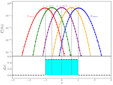
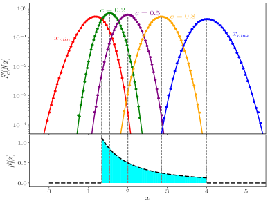
Figure 1: Top panels: Comparison of the PDFs $\derivative{F_{c}(W)}{w}$ obtained by solving numerically Eqs. (6) and (7) for different values of $c$ (solid curves) and MC simulations (markers) considering two potentials. Left panel: $v(x)=\frac{x^{2}}{2}$ that corresponds to the classical Gaussian ensemble. Right panel: $v(x)=\frac{1}{2}(x-a\log x)$, with $a>1$, inspired by the Wishart-Laguerre ensemble. A factor $N$ in the argument of $F_{c}$ has been included to magnify the size of the fluctuations. Bottom panels: Density of the 1d CGs using the same potentials, comparing the MC samples (cyan histogram) with the analytic expression for $\rho_{\textrm{eq}}(x)$ of Eq. (13) (black dashed curve). The dashed vertical lines indicate the position for which the typical fluctuations were calculated. We used $10^{6}$ MC steps for a system of $N=500$ particles.

To study the large deviation regime for which $\absolutevalue{w-x_{i}}\sim\order{1}$, for any $i=1,\dots,N$ we use the Coulomb fluid method Dean and Majumdar (2006); Vivo et al. (2007); Dean and Majumdar (2008); Majumdar and Vergassola (2009); Majumdar et al. (2009); Katzav and Pérez Castillo (2010); Majumdar et al. (2011); Mohd Ramli et al. (2012); Majumdar and Vivo (2012); Allez et al. (2013); Majumdar et al. (2013); Majumdar and Schehr (2014); Pérez Castillo (2014); Pérez Castillo et al. (2014); Melo and Pérez Castillo (2015); Pérez Castillo (2016) to compute $\varrho(c,w)\equiv\textrm{Prob}[\mathcal{C}_{w}=c]$, with $\mathcal{C}_{w}=\frac{1}{N}\sum_{j=1}^{N}\Theta(w-x_{j})$, which corresponds to the probability that exactly $cN$ particles have positions smaller than $w$. We start by writing

$$\varrho(c,w)=\frac{1}{\Omega_{0}}\int\differential{\mathbf{x}}p(\mathbf{x})\ \delta\quantity(c-\frac{1}{N}\sum_{i=1}^{N}\Theta(w-x_{i}))\,,$$ (10)

with $p(\mathbf{x})=\frac{1}{\Omega_{0}}e^{-\mathscr{H}(\mathbf{x})}$. This can be written as the following path integral (and two integrals over variables $\mu$ and $\nu$) $\varrho(c,w)=\frac{1}{\Omega_{0}}\int D[\rho,\mu,\nu]e^{-N^{3}\mathcal{S}[\rho,\mu,\nu]}$ with $\mathcal{S}$ being the action Note (1)

$$\mathcal{S}[\rho,\mu,\nu]=\int\differential{x}\rho(x)v(x)-\frac{\alpha}{2}\int\differential{x}\differential{x^{\prime}}\absolutevalue{x-x^{\prime}}\rho(x)\rho(x^{\prime})\\ -\mu\quantity(1-\int\differential{x}\rho(x))-\nu\quantity(c-\int\differential{x}\Theta(w-x)\rho(x))\,.$$ (11)

Here, $\mu$ and $\nu$ are Lagrange Multipliers to enforce normalization in the density $\rho$ and that a fraction $c$ of particles are to the left of $w$, respectively. Similarly, the normalization constant can be written as $\Omega_{0}=\int D[\rho_{0},\mu_{0}]e^{-N^{3}\mathcal{S}_{0}[\rho_{0},\mu_{0}]}$ and corresponds, in turn, to a CG without a wall. In the thermodynamic limit both expressions can be evaluated by the saddle-point method obtaining $\varrho(c,w)\asymp e^{-N^{3}\psi(c,w)}$ where

$$\psi(c,w)=\mathcal{S}[\rho^{*},\mu^{*},\nu^{*}]-\mathcal{S}_{0}[\rho^{*}_{0},\mu^{*}_{0}]$$ (12)

is the rate function. Here $\rho^{*}(x)$ corresponds physically to the equilibrium particle density of a system constrained to have a fraction of particles $c$ to the left of $w$, while $\rho_{0}^{*}(x)$ is the unconstrained equilibrium particle density. As noted in Pérez Castillo (2014, 2016), the rate function $\psi(c,w)$ has a dual role, for it describes the large deviations of $\mathcal{C}_{w}$, when $w$ is taken as a parameter or, conversely, the statistics of the $i$-th particle when $\psi$ is viewed as a function of $w$.
Noteworthy, the stationarity conditions of $\mathcal{S}$ yield an integral equation that can be solved exactly for any external potential $v(x)$. The solution for the unconstrained system is Note (1):

$$\rho_{0}^{*}(x)=\frac{v^{\prime\prime}(x)}{2\alpha}\mathbb{I}[x_{-}\leq x\leq x_{+}]\,,$$ (13)

where $\mathbb{I}[A]$ is an indicator function, whose value is $1$ whenever condition $A$ is true. The bottom panels of Fig. 1 show a comparison of this formula with unconstrained MC samplings.

From a physical perspective, we expect the constrained density to be similar to $\rho_{0}^{*}(x)$ since by placing a barrier at $w$ there will only be a local density rise in its vicinity. This is a consequence of the regularity of the 1d inter-particle potential when particles overlap, in contrast with its 2d counterpart. Hence we have that once the wall is present, there will be an accumulation of particles next it, whose magnitude depends on the fraction of the particles “pushed” by it, compared to the one of the unconstrained system. The latter one, denoted as $c^{*}(w)$, is easily calculated by integrating $\rho_{0}^{*}(x)$ up to $w$. When $w\in[x_{-},x_{+}]$ we have $c^{*}(w)=\frac{v^{\prime}(w)+\alpha}{2\alpha}$ and the constrained equilibrium density results into Note (1):

$$\rho^{*}(x)=\frac{v^{\prime\prime}(x)}{2\alpha}\left(\mathbb{I}[x_{-}\leq x\leq a]+\mathbb{I}[b<x\leq x_{+}]\right)\\ +\absolutevalue{c-c^{*}(w)}\ \delta(w-x)\,.$$ (14)

Here, the several parameters involved in Eq. (14) are defined as follows: $x_{0}$ is such that $v^{\prime}(x_{0})=\alpha(2c-1)$; when $c>c^{*}(w)$ we must take $a=w$ and $b=x_{0}$, while for $c<c^{*}(w)$ we have instead that $a=x_{0}$ and $b=w$ . For $c=c^{*}(w)$, the wall becomes ineffective, and therefore $x_{0}=w$, recovering the unconstrained solution $\rho^{*}_{0}(x)$. Finally, for $w<x_{-}$ (resp. $w>x_{+}$) we have that $c^{*}=0$ (resp. $c^{*}=1$) and similar expressions for $\rho^{*}(x)$ apply. The fact that the resulting equilibrium density has, in general, an infinitely sharp peak at $w$ as well as a non-compact and bounded support resembles some well known results for the spectral densities of RMT Dean and Majumdar (2006); Vivo et al. (2007); Dean and Majumdar (2008); Majumdar and Vergassola (2009); Majumdar et al. (2009); Katzav and Pérez Castillo (2010); Majumdar et al. (2011); Mohd Ramli et al. (2012); Majumdar and Vivo (2012); Allez et al. (2013); Majumdar et al. (2013); Majumdar and Schehr (2014); Pérez Castillo (2014); Pérez Castillo et al. (2014); Melo and Pérez Castillo (2015); Pérez Castillo (2016). However, in those systems the effect of introducing the wall significantly modifies the unconstrained density and obtaining an analytical expression for $\rho^{*}(x)$ is only possible in few, exemplary cases. Surprisingly, this is not longer true for 1d CG, where we have found the equilibrium density for any convex potential and any fraction of particles to the left of $w$. It is important to mention that so long as $v(x)$ is strong enough to dominate as $\absolutevalue{x}\to\infty$, the equilibrium densities of Eqs. (13) and (14) are the unique minimizers of the corresponding actions Chafaï et al. (2014), while the convexity of the potential assures that they are non-negative functions.

Putting these results together and evaluating Eq. (12) yields a rather simple expression for the rate function

$$\begin{split}\psi(c,w)&=\frac{\absolutevalue{c-c^{*}(w)}v(w)}{2}-\int_{a}^{b}\differential{x}\frac{v^{\prime\prime}(x)v(x)}{4\alpha}\\ &-\frac{\mu^{*}-\mu^{*}_{0}+\nu^{*}c}{2}\,,\end{split}$$ (15)

whenever the wall is inside the natural support $w\in[x_{-},x_{+}]$ (analogous expressions for $w\not\in[x_{-},x_{+}]$ together with explicit formulas are given in Note (1)). Fig. 2 shows a comparison of the analytical value of $\psi(c,w)$ and MC estimations of the rate function for the same two potentials used above. Importantly, through Eq. (15) we can recover straightforwardly the results of Dhar et al. (2017); Cunden et al. (2017) for the rate functions $\phi^{(\pm)}_{M}$ and $\phi^{(\pm)}_{m}$ controlling the left and right deviations of the rightmost and leftmost particles (see Note (1) for details). The left panels’ insets of Fig. 2 show the comparison of the rate functions of extremal particles with MC simulations, while the ones in the right panels depict a histogram obtained by MC sampling and the analytical expression for $\rho^{*}(x)$ according to Eq. (14). In all cases, the agreement is outstanding. Thus Eq. (15) provides a general and exact expression for the rate function of one-dimensional CGs and it constitutes the main result of this second part.

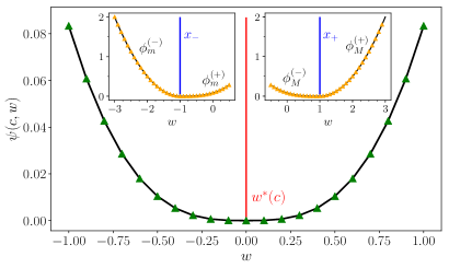
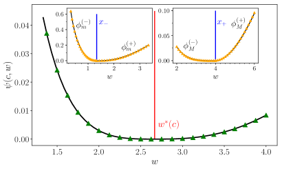
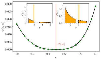
Figure 2: Left panels: Comparison between MC simulations (triangular markers) of $\psi(c,w)$ and the exact expression of Eq. (15) (solid curves) as a function of $w$. The upper panel shows the results using the harmonic potential with $\alpha=1$ and $c=0.5$, while the lower one corresponds to the Wishart-Laguerre potential with $\alpha=0.25$, $a=2$ and $c=0.75$. The right (resp. left) inset shows $\phi_{M}(w)$ (resp. $\phi_{m}(w)$), the rate function for $x_{\textrm{max}}$ (resp. $x_{\textrm{min}}$). The MC estimations of, $\phi_{M}^{(-)}(w)$ and $\phi_{m}^{{(+)}}(w)$ have been scaled as $N^{3}$, while the other rate functions were scaled as $N^{2}$. Right panels: $\psi(c,w)$ as a function of $c$, fixing $w=0.2$ for the harmonic potential (upper panel) and $w=2$ for the Wishart-Laguerre one (lower panel). The insets compare MC samples of the constrained density $\rho^{*}(x)$ (orange histograms) with the exact formula (14) (blue dashed curve), using $c=0.75$ in all the cases.

As it can be explicitly verified from Eq. (15) the rate function of the 1d CG has the noticeable feature that its first two partial derivatives vanish at $c^{*}$ and $w^{*}$, where this latter quantity is obtained by inverting the relation defining $c^{*}$. This is in stark contrast with the analogous result in RMT, where the second partial derivatives are different from zero, meaning that the fluctuations of $x_{i}$ around $w^{*}$ (resp. $\mathcal{C}_{w}$ around $c^{*}$) are of Gaussian type O’Rourke (2010); Gustavsson (2005). Instead, in the 1d case we found that the third derivatives correspond to the first non-vanishing term in the expansion of $\psi(c,w)$ around $c^{*}$ and $w^{*}$. In fact, we have that

$$\Pr(x_{i}=w)\asymp\exp(-\frac{N^{3}(v^{\prime\prime}(w^{*}))^{2}}{12\alpha}\absolutevalue{w-w^{*}}^{3})\,,$$ (16)

which is straightforward to verify that matches exactly with the asymptotic expansion of $F^{\prime}_{c=iN}(W)$ of Eq. (9). This last expression implies that the rate function is not analytical around its minimum, which is flatter than a quadratic one because of the vanishing second derivatives. We thus end up with the unusual case of having a rate function that is not strictly convex nor analytic near its minimum, once again differing from the features of the 2d CG. This is not a minor difference indeed, for it is known Touchette (2009); Ellis (1995) that a rate function that is not strictly convex can not be extended to the regime of typical fluctuations as in 2d case Pérez Castillo (2016). In other words, the 1d CG follows a weak large deviations principle, for the rate function cannot be expanded to match smoothly the typical fluctuations regimeTouchette (2009). A similar behavior has been found in the 2D Ising system Ioffe (1994); Kastner (2002); Touchette (2009) as well as for a drifted Brownian motion Nyawo and Touchette (2016). In Note (1) we provide further evidence that $\psi(c,w)$ does not provide the correct description in the regime of typical fluctuations. As a final remark, our results showed that the rate function for bulk particles in 1d CG exhibits a discontinuity in its third derivate and, while analogous results for extremal particles seem to indicate the presence of a phase transition, this feature does not necessarily carry over for bulk particles as fluctuations behave in the same way at each side of the optimal value $x^{*}$, as can be observed in Eqs. (9) and (16). Thus a phase transition for bulk particles, if any, must lie on another explanation.