Computing Resonant Inelastic X-Ray Scattering Spectra Using The Density Matrix Renormalization Group Method

Abstract

We present a method for computing resonant inelastic x-ray scattering (RIXS) spectra in one-dimensional systems using the density matrix renormalization group (DMRG) method. By using DMRG to address the problem, we shift the computational bottleneck from the memory requirements associated with exact diagonalization (ED) calculations to the computational time associated with the DMRG algorithm. This approach is then used to obtain RIXS spectra on cluster sizes well beyond state-of-the-art ED techniques. Using this new procedure, we compute the low-energy magnetic excitations observed in Cu $L$-edge RIXS for the challenging corner shared CuO₄ chains, both for large multi-orbital clusters and downfolded $t$-$J$ chains. We are able to directly compare results obtained from both models defined in clusters with identical momentum resolution. In the strong coupling limit, we find that the downfolded $t$-$J$ model captures the features of the magnetic excitations probed by RIXS after a uniform scaling of the spectra is taken into account.

Resonant inelastic x-ray scattering (RIXS) has emerged as a powerful and versatile probe of elementary excitations in quantum materials Ament et al. (2011); Kotani and Shin (2001). One of the most commonly used approaches for computing RIXS spectra is small cluster exact diagonalization (ED) Okada and Kotani (2001); Kourtis et al. (2012); Jia et al. (2014); Monney et al. (2013); Johnston et al. (2016); Vernay et al. (2008); Chen et al. (2010); Schlappa et al. (2018); Okada and Kotani (2006); Kuzian et al. (2012); Tsutsui and Tohyama (2016); Tohyama et al. (2015); Ishii et al. (2005); Tsutsui et al. (2003); van Veenendaal and Sawatzky (1994); Jia et al. (2012); Forte et al. (2011); Kumar et al. (2018); Wohlfeld et al. (2013). This approach is limited by the exponential growth of the Hilbert space, however, which restricts clusters to a relatively small size, thus limiting momentum resolution. For example, ED treatments of multi-orbital spin-chain systems such as the edge-shared CuGeO₃ or corner shared Sr₂CuO₃ have been limited to no more than six CuO₄ plaquettes Vernay et al. (2008); Monney et al. (2013); Kuzian et al. (2012); Lee et al. (2014); Okada and Kotani (2001), while studies carried out using downfolded singleband Hubbard (or $t$-$J$) chains have been limited to $\sim 16-22$ sites Schlappa et al. (2018); Kourtis et al. (2012); Kumar et al. (2018); Forte et al. (2011).

The density matrix renormalization group (DMRG) is the most powerful method for computing the ground state properties of strongly correlated materials in one dimension (1D) White (1992, 1993); Schollwöck (2011). Within the DMRG framework, several efficient methods are available for computing dynamical correlation functions, including: time-dependent DMRG White and Feiguin (2004); Daley et al. (2004), which computes dynamical correlation functions in the time domain with a subsequent Fourier transform into frequency space White and Affleck (2008); correction-vector methods, which compute the dynamical correlator directly in frequency space Kühner and White (1999); Jeckelmann (2002, 2008); Nocera and Alvarez (2016); continued fraction methods Hallberg (1995); Dargel et al. (2011, 2012); and Chebyshev polynomial expansion methods Holzner et al. (2011); Wolf et al. (2015). In this work, we present an efficient algorithm to compute the dynamical correlation function representing the RIXS scattering cross section with DMRG directly in frequency space. We then apply this approach to computing the Cu $L$-edge RIXS spectra of a quasi-1D corner-shared cuprate (e.g., Sr₂CuO₃, see Fig. 1b), a geometry that is challenging for ED calculations due to significant finite size effects Okada and Kotani (2001); Vernay et al. (2008); Monney et al. (2013). We consider a multi-orbital Hubbard model that retains the Cu and O orbital degrees of freedom, as well as a downfolded $t$-$J$ model. Using our DMRG-based approach, we access systems sizes beyond those accessible to ED, thus enabling us to directly compare the results obtained from the two models on large clusters with comparable momentum resolution.

The Kramers-Heisenberg formalism — In a RIXS experiment, photons with energy $\omega_{\mathrm{in}}$ and momentum ${\bf k}_{\mathrm{in}}$ ($\hbar=1$) scatter inelastically off of a sample, transferring momentum ${\bf q}={\bf k}_{\mathrm{out}}-{\bf k}_{\mathrm{in}}$ and energy $\Omega=\omega_{\mathrm{out}}-\omega_{\mathrm{in}}$ to its elementary excitations. The resonant nature of the probe arises because $\omega_{\mathrm{in}}$ is tuned to match one of the elemental absorption edges, such that it promotes a core electron to an unoccupied level of the crystal.

The intensity of the RIXS process $I({\bf q},\Omega)$ is given by the Kramers-Heisenberg formalism Ament et al. (2011); Kotani and Shin (2001), with

$$I({\bf q},\Omega)\propto|F_{f,g}|^{2}\delta(E_{f}-E_{g}+\Omega).$$ (1)

Here, $E_{g}$ and $E_{f}$ are the energies of the ground $|g\rangle$ and final states $|f\rangle$ of the system, respectively. The scattering amplitude $F_{f,g}$ is defined as

$$F_{f,g}=\langle f|\hat{D}^{\dagger}(\textbf{k}_{\mathrm{out}})\frac{1}{\omega_{\mathrm{in}}-\hat{H}_{\mathrm{ch}}+E_{g}+\mathrm{i}\Gamma}\hat{D}(\textbf{k}_{\mathrm{in}})|g\rangle,$$ (2)

where $\hat{D}({\bf k})$ is the dipole transition operator describing the core-hole excitation. In what follows, we consider the Cu $L$-edge (a Cu $2p\rightarrow 3d$ transition). In this case, the dipole operator is defined as $\hat{D}_{j}(\textbf{k})=\sum_{\sigma,\alpha}e^{i\textbf{k}\cdot\textbf{R}_{j}}\left[A^{\hat{\epsilon}}_{\alpha}\hat{d}^{\dagger}_{j,\sigma}\hat{p}_{j,\alpha,\sigma}+\textrm{h.c.}\right]$, where $d^{\dagger}_{j,\sigma}$ adds an electron to the valence band orbital ($3d_{x^{2}-y^{2}}$), and $\hat{p}_{j,\alpha,\sigma}$ destroys a spin $\sigma$ electron (creates a hole) in a core $2p_{\alpha}$ orbital on site $j$ located at $\textbf{R}_{j}$. The prefactor $A^{\hat{\epsilon}}_{\alpha}$ is the matrix element of the dipole transition between the core $2p_{\alpha}$ orbital and the valence $3d_{x^{2}-y^{2}}$ orbital, $\langle 3d_{x^{2}-y^{2},\sigma}|\hat{\epsilon}\cdot\hat{r}|2p_{\alpha,\sigma}\rangle$, which we set to $1$ for simplicity. $\Gamma$ is the inverse core-hole lifetime, and $\hat{H}_{\text{ch}}=\hat{H}+\hat{H}^{C}$, where ${H}^{C}=V_{C}\sum\limits_{j,\sigma,\sigma^{\prime}}\hat{n}^{d}_{j,\sigma}(1-\hat{n}^{p_{\alpha}}_{j,\sigma^{\prime}})$ describes the Coulomb interaction between the core hole and the valence electrons, and $\hat{H}$ is the many-body Hamiltonian of the system.

Under the assumption that the core-hole is completely localized, and only one Cu $2p_{\alpha}$ orbitals is involved in the RIXS process, Eq. (2) simplifies to

$$F_{f,g}\propto\sum\limits_{j,\sigma,\sigma^{\prime}}e^{i\textbf{q}\cdot\textbf{R}_{j}}\langle f|\hat{D}^{\dagger}_{j,\sigma}\frac{1}{\omega_{\mathrm{in}}-\hat{H}_{\mathrm{ch},j}+E_{g}+i\Gamma}\hat{D}_{j,\sigma^{\prime}}|g\rangle,$$

where we have defined the local dipole-transition operator $\hat{D}_{j,\sigma}\equiv\hat{d}^{\dagger}_{j,\sigma}\hat{p}_{j,\sigma}$ and $\hat{H}_{\mathrm{ch},j}=\hat{H}+\hat{H}^{C}_{j}$, with $\hat{H}^{C}_{j}=V_{C}\sum\limits_{\sigma,\sigma^{\prime}}\hat{n}^{d}_{j,\sigma}(1-\hat{n}^{p}_{j,\sigma^{\prime}})$.

Reformulation of the problem for DMRG — The primary difficulty in evaluating Eq. (1) lies in computing the final states $|f\rangle$. This task is often accomplished using ED on small clusters meant to approximate the infinite system. Obtaining these same final states is usually impossible with DMRG, which targets only the ground state; however, we will show that to accomplish this task one can use the Lanczos method, which projects the state onto a Krylov space Krylov (1931). Some of the present authors introduced this alternative method to calculate the correction vectors for frequency-dependent correlation functions with DMRG Nocera and Alvarez (2016).

We can formulate an efficient DMRG algorithm by expanding the square in Eq. (1), yielding a real space version of the Kramer-Heisenberg formula. To compact the notation, we define vectors $|\alpha_{j,\sigma}\rangle\equiv[\omega_{\mathrm{in}}-\hat{H}_{\mathrm{ch},j}+E_{g}+\mathrm{i}\Gamma]^{-1}\hat{D}_{j,\sigma}|g\rangle$. Using this definition, Eq. (1) can be written as

$$I(\textbf{q},\Omega)\propto-\mathrm{Im}\Bigg{[}\sum\limits_{i,j=0}^{L-1}\sum\limits_{\begin{subarray}{c}\gamma,\gamma^{\prime}\\ \sigma,\sigma^{\prime}\end{subarray}}e^{i\textbf{q}\cdot(\textbf{R}_{i}-\textbf{R}_{j})}\times$$

$$\langle\alpha_{i,\gamma}|\hat{D}_{i,\gamma^{\prime}}\frac{1}{\Omega-\hat{H}+E_{g}+\mathrm{i}\eta}\hat{D}^{\dagger}_{j,\sigma^{\prime}}|\alpha_{j,\sigma}\rangle\Bigg{]}.$$ (3)

Here, $\eta$ is a broadening parameter, which plays the same role as the Gaussian or Lorentzian broadening introduced in ED treatments of the energy-conserving $\delta$-function appearing in Eq. (1). Throughout this work, we set it to $75$ meV. Note that the vectors $|\alpha_{j,\sigma}\rangle$ must be computed for each value of $\omega_{\mathrm{in}}$ and $\Gamma$.

The X-ray absorption spectrum (XAS) can be computed using a similar formalism. Its intensity is given by

$$I(\omega_{\mathrm{in}})\propto-\mathrm{Im}\sum_{j,\sigma}\langle g|\hat{D}^{\dagger}_{j,\sigma}\frac{1}{\omega_{\mathrm{in}}-\hat{H}_{\mathrm{ch},j}+E_{g}+\mathrm{i}\Gamma}\hat{D}_{j,\sigma}|g\rangle.$$ (4)

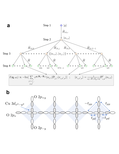
Figure 1: (a) A sketch of the algorithm for computing the real space Kramers-Heisenberg formula [Eq. (Computing Resonant Inelastic X-Ray Scattering Spectra Using The Density Matrix Renormalization Group Method)] using the DMRG method at a fixed value of the energy loss $\Omega=\omega_{l}$. (b) A sketch of the multi-orbital $pd$-model describing the corner shared spin chain cuprates (e.g. Sr₂CuO₃).

Finally, we note that we have removed the elastic line from all spectra shown in this work. The precise method for doing this is discussed in Supplementary Note IV.

Computational procedure — The algorithm to compute the RIXS spectra using Eq. (Computing Resonant Inelastic X-Ray Scattering Spectra Using The Density Matrix Renormalization Group Method) is as follows (see also Fig. 1a):

Step 1: Compute the ground state $|g\rangle$ of $\hat{H}$ using the standard ground state DMRG method. The vector $|g\rangle$ must be stored for later use.

Step 2: Restart from the ground state calculation, reading and then targeting the ground state vector calculated earlier and using a different Hamiltonian $\hat{H}_{\mathrm{ch},c}=\hat{H}+\hat{H}_{c}^{C}$, where $j=c$ is the center site of the chain. Construct the vector $|\alpha_{c,\sigma}\rangle$ at the center of the chain using the Krylov-space correction vector approach Nocera and Alvarez (2016)

$$|\alpha_{c,\sigma}\rangle \simeq\tilde{T}^{\dagger}_{c}\tilde{S}^{\dagger}_{c}\frac{1}{\omega_{\mathrm{in}}-D_{\mathrm{ch},c}+E_{g}+\mathrm{i}\Gamma}\tilde{S}_{c}\tilde{T}_{c}\hat{D}_{c,\sigma}|g\rangle,$$ (5)

where we have performed a Lanczos tridiagonalization $\tilde{T}_{c}$ with starting vector $\hat{D}_{c,\sigma}|g\rangle$, and a subsequent diagonalization $\tilde{S}_{c}$ of the Hamiltonian $\hat{H}_{\mathrm{ch},c}$ and $D_{\mathrm{ch},c}$ is its diagonal form in the Krylov basis. The vector $|\alpha_{c,\sigma}\rangle$ should also be stored for later use. Because the cluster is not periodic, the use of a central site here is an approximation that will become exact in the thermodynamic limit. This central site “trick” was used for the first time in the application of time-dependent DMRG White and Feiguin (2004).

Step 3: Restart from previous run, now using a different Hamiltonian $\hat{H}_{\mathrm{ch},j}=\hat{H}+\hat{H}_{j}^{C}$. Read and then target (in the DMRG sense) the ground state vector calculated in Step 1, as well as the vector $|\alpha_{c,\sigma}\rangle$ constructed in Step 2. For each site $j$, except for the center site considered in Step 2, construct the vector

$$|\alpha_{j,\gamma}\rangle \simeq\tilde{T}^{\dagger}_{j}\tilde{S}^{\dagger}_{j}\frac{1}{\omega_{\mathrm{in}}-D_{\mathrm{ch},j}+E_{g}+\mathrm{i}\Gamma}\tilde{S}_{j}\tilde{T}_{j}\hat{D}_{j,\gamma}|g\rangle,$$ (6)

with Lanczos tridiagonalization $\tilde{T}_{j}$ with starting vector $\hat{D}_{j,\gamma}|g\rangle$, and a subsequent diagonalization of $\hat{H}_{\text{ch},j}$. This step of the algorithm requires a number of runs which is equal to the number of sites minus $1$, i.e., $L-1$. These can be run in parallel on a standard cluster machine, restarting from Step 2. Performing Step 2 and Step 3 in this sequence is crucial for having the vectros $|\alpha_{c,\sigma}\rangle$ and $|\alpha_{j,\gamma}\rangle$ in the same DMRG basis. The vector $|\alpha_{j,\gamma}\rangle$ should also be stored for later use.

Step 4: Restart using the original Hamiltonian $\hat{H}$. Read and then target the ground state produced in Step 1, $|\alpha_{c,\sigma}\rangle$ produced in Step 2, and the vector $|\alpha_{j,\gamma}\rangle$ constructed in Step 3. For a fixed $\Omega=\omega_{l}$, compute the correction vector of $|\alpha_{c,\sigma}\rangle$ using again the Krylov-space correction vector approach as

$$| x_{c,\sigma^{\prime},\sigma}\rangle\equiv\frac{1}{\Omega-\hat{H}+E_{g}+\mathrm{i}\eta}\hat{D}^{\dagger}_{c,\sigma^{\prime}}|\alpha_{c,\sigma}\rangle$$

$$=\tilde{T}^{\dagger}\tilde{S}^{\dagger}\frac{1}{\Omega-D+E_{g}+\mathrm{i}\eta}\tilde{S}\tilde{T}\hat{D}^{\dagger}_{c,\sigma^{\prime}}|\alpha_{c,\sigma}\rangle$$ (7)

with Lanczos tridiagonalization $\tilde{T}$ (using $\hat{D}^{\dagger}_{j,\sigma^{\prime}}|\alpha_{c,\sigma}\rangle$ as the seed) and a subsequent diagonalization $\tilde{S}$ of the Hamiltonian $\hat{H}$, with $D$ being the diagonal form of $\hat{H}$ in the Krylov basis. This is a crucial part of the algorithm, which amounts to computing the correction vector $|x_{c,\sigma^{\prime},\sigma}\rangle$ of a previously calculated correction vector $|\alpha_{c,\sigma}\rangle$. Execute this computation $N_{\Omega}$ times for $\Omega\in[\omega_{0},\omega_{N-1}]$.

Step 5: Finally, compute the RIXS spectrum in real space $I_{j,c}(\Omega)\propto\langle\alpha_{j,\gamma}|\hat{D}_{j,\gamma^{\prime}}|x_{c,\sigma^{\prime},\sigma}\rangle$ and then Fourier transform the imaginary part to obtain the RIXS intensity

$$I(\textbf{q},\Omega)\propto-\mathrm{Im}\sum\limits_{\begin{subarray}{c}j,\gamma,\gamma^{\prime}\\ \sigma,\sigma^{\prime}\end{subarray}}e^{i\textbf{q}\cdot(\textbf{R}_{j}-\textbf{R}_{c})}I_{j,c}(\Omega).$$ (8)

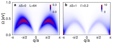
Figure 2: DMRG results for the RIXS intensity $I(q,\Omega)$ of a half-filled $t$-$J$ chain. Results are shown for a $L=64$ site chain, in the (a) $\Delta S=0$ and (b) $\Delta S=1$ channels. The remaining parameters are $t=0.3$ eV, $J=0.25$ eV, $\eta=75$ meV and $\omega_{\mathrm{in}}=0.1$ eV (which corresponds to the resonance observed in the XAS).

Computational complexity — The computational cost required for DMRG to compute the RIXS spectrum can be easily estimated, assuming that the ground state of the Hamiltonian has already been calculated. Let $C_{2-3}$ be the computational cost (i.e., the number of hours) for a single run in Step 2 ($1$ run only) or Step 3 ($L-1$ runs in total). Let $C_{4}$ be the computational cost for a single run in Step 4. The total computational time needed to compute the RIXS spectrum is then $\textrm{CPU}_{\text{cost}}=C_{2-3}L+C_{4}LN_{\Omega}$, where $N_{\Omega}$ is the number of frequencies needed in a given interval of energy losses. The use of this center site “trick” reduces the computational cost by a factor of the order of $L$ (Eq. (Computing Resonant Inelastic X-Ray Scattering Spectra Using The Density Matrix Renormalization Group Method) to Eq. (8)). For the largest system size considered in this work ($20$ plaquettes in CuO₄ multi-orbital model at half-filling, using up to $m=1000$ DMRG states), the typical values for $\textrm{CPU}_{\text{cost}}$ on a single core of a standard computer cluster are: $C_{2-3}\sim 2$ hours, while $C_{4}\sim 2-24$ hours. The computational cost $C_{4}$ for Step 4 follows the typical performance profile of the Krylov-space approach found in Ref. Nocera and Alvarez (2016), where less CPU time is needed to compute the spectra at lower energy-losses. We also note that the calculation of each energy loss is trivially parallelizable. From these assumptions, we estimate the proposed method can compute the RIXS spectrum of a cluster as large as Cu₂₀O₆₁ in less than a day if enough cores are available.

Numerical Results for the $t$-$J$ model — We first apply our approach to compute the RIXS spectrum of the 1D $t$-$J$ model as an effective model for the antiferromagnetic corner-shared spin chain cuprate Sr₂CuO₃ (see Methods). Throughout this paper, we adopt open boundary conditions and work at half-filling and set $t=0.3$ eV for the nearest neighbor hopping and $J=0.25$ eV for the antiferromagnetic exchange interaction. These values are typical for Sr₂CuO₃ Suzuura et al. (1996); Motoyama et al. (1996); Kojima et al. (1997); Schlappa et al. (2012); Walters et al. (2009); Lee et al. (2013); Bisogni et al. (2012).

Before scaling up our DMRG calculations to large systems, we benchmarked our method by directly comparing our DMRG results to ED. The results for a $L=16$ sites $t$-$J$ chain are presented in Supplementary Note I. (We provide a similar comparison for a four-plaquette multi-orbital cluster in Supplementary Note II.) Our DMRG approach gives perfect agreement with the ED result for both the XAS and RIXS spectra, for the largest clusters we can access with ED. All of the DRMG simulations presented in this work used up to $m=1000$ states, with a truncation error smaller than $10^{-6}$.

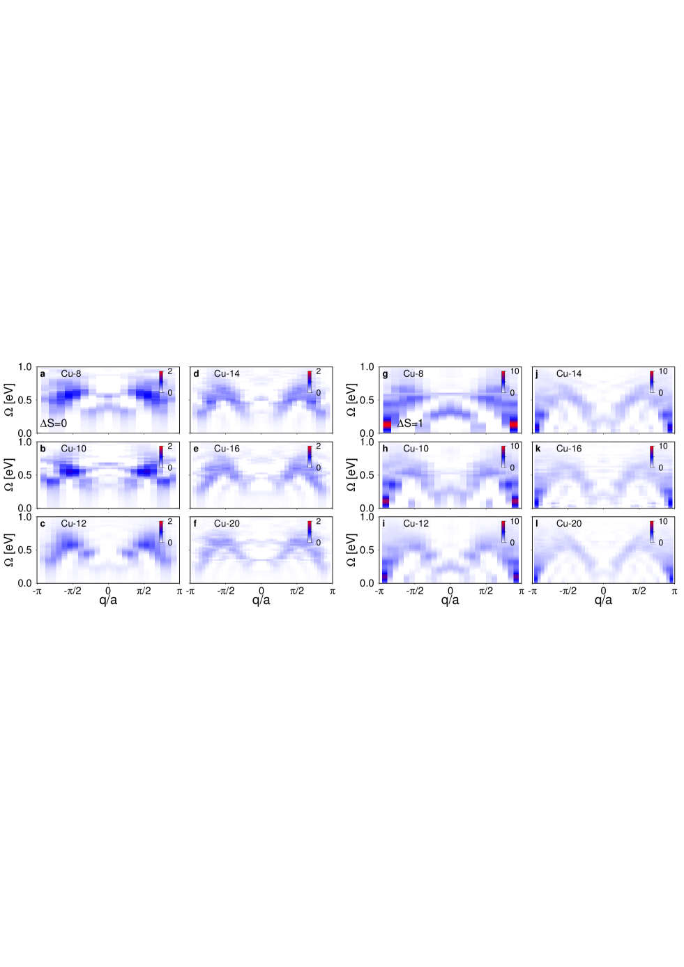
Figure 3: The response $I(q,\Omega)$ obtained with DMRG for a multi-orbital pd model as a function of the number of CuO₄ plaquettes. Panels (a)-(f) show the spin-conserving $\Delta S=0$ channel to the RIXS intensity, while panels (g)-(l) show the non-spin-conserving $\Delta S=1$ channel. Results are shown for 8 to 20 unit cells at half filling, computed at resonance with $\omega_{\mathrm{in}}=2.5$, $\Gamma=0.2$, and $V_{C}=4.0$.

We now turn to results obtained on a $L=64$ site chain, as shown in Fig. 2. Here, we present results for the spin-flip ($\Delta S=1$) and non-spin-flip ($\Delta S=0$) contributions to the total RIXS intensity. The $\Delta S=0$ contribution corresponds to the $\sigma=\sigma^{\prime}$ and $\gamma=\gamma^{\prime}$ terms in the Kramers-Heisenberg formula Eq. (Computing Resonant Inelastic X-Ray Scattering Spectra Using The Density Matrix Renormalization Group Method). In this case, only two configurations ($\gamma=\gamma^{\prime}=\sigma=\sigma^{\prime}=\uparrow$ and $\gamma=\gamma^{\prime}=\downarrow$, $\sigma=\sigma^{\prime}=\uparrow$) have to be explictly calculated with DMRG, as the other two possible spin conserving configurations contribute equally by symmetry. The remaining terms with $\sigma\neq\sigma^{\prime}$ and $\gamma\neq\gamma^{\prime}$ determine the non-spin conserving $\Delta S=1$ contributions to the spectrum. In this case, only one configuration ($\sigma^{\prime}=\downarrow$, $\sigma=\uparrow$, $\gamma^{\prime}=\downarrow$, $\gamma=\uparrow$) has been simulated with DMRG, as the flipped configuration ($\sigma^{\prime}=\uparrow$, $\sigma=\downarrow$, $\gamma^{\prime}=\uparrow$, $\gamma=\downarrow$) contributes equally by symmetry. The remaining two possible non-spin conserving configurations also give zero contribution to the RIXS spectrum by symmetry.

In Fig. 2, the $\Delta S=1$ part of the RIXS spectrum shows a continuum of excitations resembling the two spinon continuum commonly observed in the dynamical spin structure factor $S(q,\omega)$ of one-dimensional spin-$1/2$ antiferromagnets Tennant et al. (1995); Lake et al. (2005); Mourigal et al. (2013); Lake et al. (2013). The $\Delta S=0$ contribution in Fig 2a shows two broad arcs with maxima at $q=\pi/2a$. Notice also a perfect cancellation of the RIXS signal at the zone boundary, which is $q=\frac{\pi}{a}\frac{L}{L+1}$ in open boundary conditions. Our results agree with the ED results of Refs. Kourtis et al., 2012 and Forte et al., 2011, but with much better momentum resolution. We find that the finite size effects of the magnetic excitations in the $t$-$J$ model are mild; we observe only small differences between results obtained on $L=32$ (not shown in Fig. 2) and $L=64$ site clusters.

Magnetic excitations in the multi-orbital $pd$-model — In the strong coupling limit, the low-energy magnetic response of the spin-chain cuprates are believed to be effectively described by a single orbital Hubbard or $t$-$J$ model Emery (1987); Zhang and Rice (1988). According to this picture, holes predominantly occupy the Cu orbitals at half-filling, while the oxygens along the Cu-Cu direction provide a pathway for superexchange interactions between the nearest-neighbor Cu orbitals. Since our DMRG approach provides access to large cluster sizes, we now compute the RIXS spectrum of a more realistic multi-orbital model. Here, we consider the challenging corner-shared geometry, which suffers from slow convergence in the cluster size. To address this, we consider finite 1D Cu_nO_3n+1 clusters, with open boundary conditions, as illustrated in Fig. 1b for the $n=4$ case. The Hamiltonian is given in the Methods section. We evaluated the Cu $L$-edge RIXS intensity for this model as a function of $n$ for up to $n=20$ CuO₄ plaquettes.

The RIXS spectra for spin-conserving ($\Delta S=0$) and non-spin-conserving contributions ($\Delta S=1$) calculated with our DMRG method are shown in Fig. 3. Similar to the $t-J$ spectra, panels (a-f) in Fig. 3 show two broad arcs with maxima at $\pm\pi/2a$. Here, we observe significant finite size effects in the RIXS spectra. Some of these effects are the result of our use of the “center-site approximation” in evaluating the Kramers-Heisenberg formula. For example, the downward dispersing low-energy peak centered at $q=0$ seen in the smaller clusters is the result of this approximation. These features in the spectra can be minimized by carrying out calculations on larger clusters. Because of this, to observe well defined spectral features, we need to consider at least fourteen plaquettes. The pd model also shows that the low-energy $\Delta S=1$ part of the RIXS spectrum is characterized by a two-spinon-like continuum of excitations (panels (g-l) in Fig. 3).

Comparing the multi-orbital and effective $\boldmath{t}$-$\boldmath{J}$ models — Over the past decade, there has been a considerable research effort dedicated to quantitatively understand the intensity of magnetic excitations probed by inelastic neutron scattering (INS) Nagler et al. (1991); Walters et al. (2009); Mourigal et al. (2013). This effort is motivated by the desire to understand the relationship between the spectral weight of the dynamical spin response $S({\bf q},\omega)$ and the superconducting transition temperature T_c of unconventional superconductors Scalapino (2012). To this end, several studies have set out to determine whether the observed INS intensity can be accounted for by the Heisenberg model in low-dimensional strongly correlated cuprates. Here, the highest degree of success has been achieved in quasi-1D materials, where accurate theoretical predictions for $S(q,\omega)$ are available Walters et al. (2009); Mourigal et al. (2013). Many of these studies find that the low-energy Heisenberg model can indeed account for the INS intensity, after accounting for corrections due to effects such as the degree of covalency, its impact on the form factor, and Debye-Waller factors.

RIXS has also been applied to study magnetic excitations in many of the same materials Schlappa et al. (2012, 2018); Bisogni et al. (2012). It is therefore natural to ponder how covalency modifies the magnetic excitations as viewed by RIXS. In the limit of a short core-hole lifetime, or under constraints in the incoming and outgoing photon polarization, the RIXS intensity for single orbital Hubbard and $t$-$J$ chains is well approximated by $S(q,\omega)$ Jia et al. (2014); Forte et al. (2011); Bisogni et al. (2012); Ament et al. (2011). However, to the best of our knowledge, no systematic comparison of the RIXS intensity, as computed by the Kramers-Heisenberg formalism, has been carried out for multi-orbital and downfolded Hamiltonians.

Figure 3 demonstrates that DMRG grants access to large system sizes. We are, therefore, in a position to make such a comparison for the multi-orbital spin-chain cuprates. Figure 4 compares the spectra computed on a $L=20$ site $t$-$J$ chain against those computed on a Cu₂₀O₆₁ cluster, such that the momentum resolution of the two clusters is the same. The parameters for the multi-orbital model are identical to those used in Fig. 3. To facilitate a meaningful comparison with the $t$-$J$ model, we adopted $t=0.5$ eV and $J=0.325$ eV. These values are obtained by diagonalizing a Cu₂O₇ cluster (see methods). Note that we use the same value of the core hole potential $V_{C}=4$ eV in both cases. In supplementary note III, we show results for a reduced value of $V_{C}$ for the $t$-$J$ model, which are very similar. To compare the two spectra, the results for the $t$-$J$ model have been scaled by a factor of $0.26$ such that the maximum intensity of the $\Delta S=1$ excitations is the same at the zone boundary. This factor presumably accounts for covalent factors and differences in how the core-hole interacts with the distribution of electrons in the intermediate state.

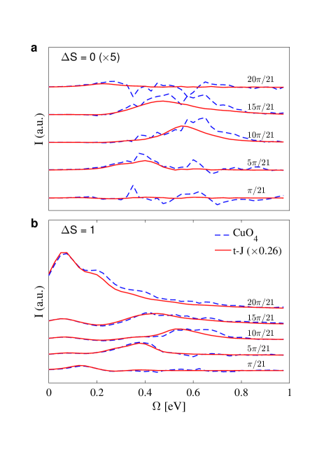
Figure 4: A comparison of the magnetic RIXS excitations computed using DMRG for a 20-site $t$-$J$ chain (solid red line) and multi-orbital pd model (dashed blue line) with twenty unit cells at half filling. Results are shown for the (a) $\Delta S=0$ and (b) $\Delta S=1$ channels. The parameters for the $t$-$J$ model are $t=0.5$ eV, $J=0.325$ eV, $V_{C}=4$ eV, $\Gamma=0.2$ eV, and $\omega_{\mathrm{in}}=0.14$ eV. The parameters for the multi-orbital model are given in the main text. The incident photon energy is $\omega_{\mathrm{in}}=2.5$ eV, the inverse core hole lifetime is $\Gamma=0.2$ eV, and the core hole potential is $V_{C}=4$ eV. The results for the $t$-$J$ model have been scaled by a factor of $0.26$ such that the maximum intensity of the $\Delta S=1$ excitations are the same at the zone boundary.

After we have rescaled the spectra, we find excellent overall agreement between the two calculations: the amplitude of the broad arcs for the magnetic excitations, both in the $\Delta S=0$ and in $\Delta S=1$ channels of the RIXS spectra are well captured by the $t$-$J$ model. There are, however, minor quantitative differences related to the spectral weight of the excitations appearing near $q=\pi/2a$ in the $\Delta S=0$ channel. For example, the $t$-$J$ model concentrates the magnetic excitations at slightly lower values of the energy loss in $\Delta S=0$ channel. This discrepancy might be compensated for by taking a different value of $J$; however, this would come at the expense of the agreement in the $\Delta S=1$ channel. These differences should be kept in mind when one calculates the low-energy magnetic RIXS spectra using an effective $t$-$J$ or single-band Hubbard model. Nevertheless, our results show that in the strong coupling limit, the magnetic RIXS spectrum can be described well by the effective $t$-$J$ model.

Figure 4 shows that that the overall agreement between the full multi-orbital model and the $t$-$J$ model is much better in the $\Delta S=1$ channel than in the $\Delta S=0$ channel. We can naively understand this difference by recalling the role of charge fluctuations in the two magnetic excitation pathways. The $\Delta S=1$ RIXS excitations are possible in a system with strong spin-orbit coupling in the Cu $2p$ orbitals, which allows the spin of the core-hole to flip in the intermediate state of the RIXS process Forte et al. (2011); Schlappa et al. (2018); Kourtis et al. (2012). The $\Delta S=0$ pathway, however, requires a double spin-flip between neighboring Cu spins in the final state Forte et al. (2011); Kourtis et al. (2012). At the Cu $L$-edge, such processes occur due to charge fluctuations between the neighboring Cu sites in the intermediate state. The multi-orbital model treats such charge fluctuations differently owing to the presence of the ligand oxygen orbitals. This difference accounts for the discrepancy between the two models in the $\Delta S=0$ channel. At the Cu $L$-edge, however, the strong core-hole potential suppresses this difference by repelling holes from the site where it was created resulting in only minor differences between the predictions of the two models.

Concluding Remarks — We have presented a novel DMRG approach to computing the RIXS spectra and benchmarked this method against traditional ED. Using our DMRG algorithm, we can compute the RIXS spectra on 1D clusters much larger than those accessible to state-of-the-art ED methods. Using this method, we modeled the magnetic excitations probed by RIXS at the Cu $L$-edge in 1D antiferromagnets on the largest cluster sizes to date. We found that both the full multi-orbital cluster and the effective $t$-$J$ model provide comparable descriptions of the excitations in the $\Delta S=1$ channel, while there were minor quantitative differences in the $\Delta S=0$ channel. These differences could be explained by noting the difference in the way that these two channels probe magnetic excitations. Finally, we note that the bottleneck to RIXS simulations using ED is the exponential growth of the Hilbert space. Our approach shifts the computational burden to the availability of CPUs thus opening the door to calculations for large systems. For example, one can envision extending this approach to the quasi-2D models currently under active study by the DMRG community.

Methods — The multi-orbital $pd$-Hamiltonian describing the corner-shared spin-chains, given in the hole-picture, is

$$H =\epsilon_{d}\sum\limits_{i,\sigma}n^{d}_{i,\sigma}+\sum_{j,\sigma}\epsilon_{p,\gamma}n^{p}_{j,\gamma,\sigma}+\sum\limits_{\begin{subarray}{c}\langle i,j\rangle\\ \gamma,\sigma\end{subarray}}t_{pd}^{ij}(d^{\dagger}_{i,\sigma}p_{j,\gamma,\sigma}+\textrm{h.c.})$$ (9)

$$+\sum\limits_{\begin{subarray}{c}\langle j,j^{\prime}\rangle\\ \gamma,\gamma^{\prime},\sigma\end{subarray}}t_{pp}^{jj^{\prime}}p^{\dagger}_{j,\gamma,\sigma}p_{j^{\prime},\gamma^{\prime}\sigma}+U_{d}\sum\limits_{i}n^{d}_{i,\uparrow}n^{d}_{i,\downarrow}$$

$$+U_{p}\sum\limits_{i,\gamma}n^{p}_{j,\gamma,\uparrow}n^{p}_{j,\gamma,\downarrow}+U_{pd}\sum\limits_{\begin{subarray}{c}\langle i,j\rangle\\ \sigma,\sigma^{\prime}\end{subarray}}n^{d}_{i,\sigma}n^{p}_{j,\gamma,\sigma^{\prime}}.$$

Here, $\langle\dots\rangle$ denotes a sum over nearest neighbor orbitals; $d^{\dagger}_{i,\sigma}$ ($p^{\dagger}_{j,\gamma,\sigma}$) creates a spin $\sigma$ hole on the $i^{\mathrm{th}}$ Cu 3$d_{x^{2}-y^{2}}$ orbital (the $j^{\mathrm{th}}$ O 2$p_{\gamma}$ orbital, $\gamma=x$, $\pm y$); $\epsilon_{d}$ and $\epsilon_{p}$ are the on-site energies; $n^{d}_{i,\sigma}$ ($n^{p}_{j,\gamma,\sigma}$) is the number operator for the Cu 3$d_{x^{2}-y^{2}}$ orbital (the $j^{\mathrm{th}}$ O 2$p_{\gamma}$ orbital); $t_{pd}^{ij}$ and $t_{pp}^{j,j^{\prime}}$ are the Cu-O and O-O overlap integrals, respectively; $U_{d}$ and $U_{p}$ are the onsite Hubbard repulsions of the Cu and O orbitals, respectively, and $U_{pd}$ is the nearest-neighbor Cu-O Hubbard repulsion. The phase convention for the overlap integrals is shown in Fig. 1b. In this work, we adopt (in units of eV) $\epsilon_{d}=0$, $\epsilon_{p,x}=3$, $\epsilon_{p,y}=3.5$, $|t_{(p,x)d}|=1.5$ $|t_{(p,y)d}|=1.8$, $|t_{pp}|=0.75$, $U_{d}=8$, $U_{p}=4$, and $U_{pd}=1$, following Ref. Wohlfeld et al., 2013.

In the limit of large $U_{d}$, one integrates out the oxygen degrees of freedom and maps Eq. (9) onto an effective spin-$1/2$ $t$-$J$ Hamiltonian Zhang and Rice (1988)

$$H=-t\sum_{i,\sigma}(\tilde{d}_{i,\sigma}^{\dagger}\tilde{d}_{i+1,\sigma}^{\phantom{\dagger}}+h.c.)+J\sum_{i}\textbf{S}_{i}\cdot\textbf{S}_{i+1}.$$

Here, $\tilde{d}_{i,\sigma}$ is the annihilation operator for a hole with spin $\sigma$ at site $i$, under the constraint of no double occupancy, $n_{i}=\sum_{\sigma}n_{i,\sigma}$ is the number operator, and $\textbf{S}_{i}$ is the spin operator at site $i$.

To facilitate a direct comparison between the two models, one can extract the hopping $t$ and exchange interaction $J$ from an ED calculation of a two-plaquette Cu₂O₇ cluster with open boundary conditions Johnston et al. (2009). Here, we obtain the hopping ($t=0.5$ eV) by diagonalizing cluster in the ($2\uparrow,1\downarrow$)-hole sector, and setting $2t$ to be equal to the energy separation between the bonding and antibonding states of the Zhang-Rice singlet. Similarly, we can obtain the superexchange ($J=0.325$ eV) by diagonalizing the cluster in the $(1\uparrow,~{}1\downarrow)$-hole sector, and setting the singlet-triplet splitting of the Cu ($d^{9}d^{9}$) configurations equal to $J$.

Acknowledgements — A. N. and E. D. were supported by the U.S. Department of Energy, Office of Basic Energy Sciences, Materials Sciences and Engineering Division. G. A. and S. J. were supported by the Scientific Discovery through Advanced Computing (SciDAC) program funded by the U.S. Department of Energy, Office of Sciences, Advanced Scientific Computing Research and Basic Energy Sciences, Division of Materials Sciences and Engineering. This research used computational resources supported both by the University of Tennessee and Oak Ridge National Laboratory Joint Institute for Computational Sciences (Advanced Computing Facility). It also used computational resources at the National Energy Research Scientific Computing Center (NERSC).

Supplementary Note I:   Supplementary Note I: Benchmarks on a 16-site $t$-$J$ chain

In this note, we compare the results of our DMRG method against the spectrum obtained from Lanczos ED. Supplementary Figure 1 directly compares the results from the two methods applied to a $L=16$ site $t$-$J$ chain, where our DMRG approach gives perfect agreement with the ED results for both the XAS and RIXS spectra. Here, we have assumed parameter values typical for a Cu $L$-edge measurement performed on Sr₂CuO₃ with $t=0.3$, $J=0.25$, an inverse core hole lifetime $\Gamma=0.3$ eV, and a core-hole repulsion $V_{C}=2.0$ eV. The two methods give a resonant absorption peak in the XAS for an incident energy $\omega_{\mathrm{in}}=0.1$ eV. Note that in this comparison we did not use the center trick for calculating the RIXS spectra. Instead, Eq. (3) of the main text has been used.

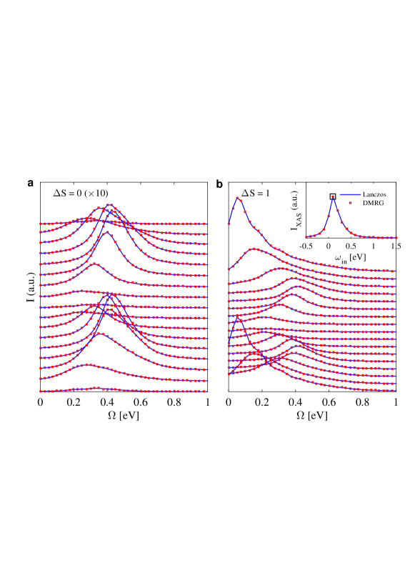
Supplementary Figure 1: A comparison of the RIXS response $I(q,\Omega)$ calculated for a $t$-$J$ chain of length $L=16$ at half filling $N=16$ with $J=0.25$ eV and $t=0.3$ eV. Results are shown for both the (a) $\Delta S=0$ and (b) $\Delta S=1$ channels, computed at resonance with $\omega_{\mathrm{in}}=0.1$ eV. We have computed the spectrum with DMRG (red squares), which we compare to results obtained from Lanczos ED (solid blue line). The inset of panel (b) compares the XAS spectrum computed with DMRG [using Eq. (8)] and Lanczos ED. The open black box indicates the incident energy $\omega_{\mathrm{in}}$ used to compute the RIXS spectra. Note that in this comparison we did not use the center trick for calculating the RIXS spectra. Instead, Eq. (3) of the main text has been used.

Supplementary Note II:   Supplementary Note II: Benchmarks on a multi-orbital corner-shared CuO₄ chain

Supplementary Figure 2 presents a second comparison of the results obtained from a multi-orbital Cu₄O₁₃ cluster, with open boundary conditions. The model parameters are the same as those used in the main text. Our DMRG approach again gives perfect agreement with the ED result for both the XAS and RIXS spectra.

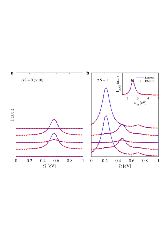
Supplementary Figure 2: A comparison of the RIXS response $I(q,\Omega)$ calculated for a multi-orbital pd model for Sr₂CuO₃ with 4 unit cells at half filling $N=4$. The model parameters are identical to those used in the main text. Results are shown for both the (a) $\Delta S=0$ and (b) $\Delta S=1$ channels, computed at resonance with $\omega_{\mathrm{in}}=2.5$ eV. The spectrum computed with DMRG (red squares) is compared with results obtained from Lanczos ED (solid blue line). The inset of panel (b) shows a comparison of the XAS spectrum computed with DMRG [using Eq. (8)] and Lanczos ED. The open black box indicates the incident energy $\omega_{\mathrm{in}}$ used to compute the RIXS spectra. Note that in this comparison we did not use the center trick for calculating the RIXS spectra. Instead, Eq. (3) of the main text has been used.

Supplementary Note III:   Supplementary Note III: Comparison of the Two Models

In the main text, we compared results for the magnetic RIXS spectra of the $t$-$J$ and multi-orbital $pd$ model, each with 20 unit cells. Here, Supplementary Figure 3 presents a similar comparison but for a different value of the core-hole potential used for the $t$-$J$ model.

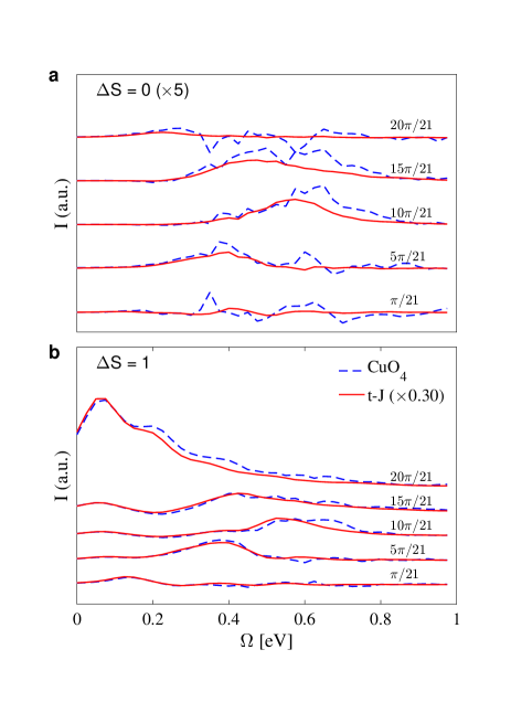
Supplementary Figure 3: A comparison of the magnetic RIXS excitations computed using DMRG for a 20-site $t$-$J$ chain (solid red line) and multi-orbital pd model (dashed blue line) with twenty unit cells at half filling. Results are shown for the (a) $\Delta S=0$ and (b) $\Delta S=1$ channels. The parameters for the $t$-$J$ model are $t=0.5$ eV, $J=0.325$ eV and $\omega_{\mathrm{in}}=0.04$ eV. The parameters for the multi-orbital model are given in the main text. The incident photon energy is $\omega_{\mathrm{in}}=2.5$ eV, the inverse core hole lifetime is $\Gamma=0.2$ eV, and the core hole potential is $V_{C}=2$ eV. The results for the $t$-$J$ model have been scaled by a factor of $0.30$ such that the maximum intensity of the $\Delta S=1$ excitations is the same at the zone boundary.

Supplementary Note IV:   Supplementary Note IV: Removing the Elastic Line From the DMRG Calculations

We first rewrite Eq. (3) of the main text to explicitly indicate the center site $c$

$$I(\textbf{q},\Omega)\propto-\mathrm{Im}\Bigg{[}\sum\limits_{i=0}^{L-1}\sum\limits_{\begin{subarray}{c}\gamma,\gamma^{\prime}\\ \sigma,\sigma^{\prime}\end{subarray}}e^{i\textbf{q}\cdot(\textbf{R}_{i}-\textbf{R}_{c})}\langle\alpha_{i,\gamma}|\hat{D}_{i,\gamma^{\prime}}\frac{1}{\Omega-\hat{H}+E_{g}+\mathrm{i}\eta}\hat{D}^{\dagger}_{c,\sigma^{\prime}}|\alpha_{c,\sigma}\rangle\Bigg{]}.$$ (1)

The $\Delta S=0$ contribution computed with DMRG is then given by the expression

$$I_{\Delta S=0}(\textbf{q},\Omega)\propto-\mathrm{Im}\Bigg{[}\sum\limits_{i=0}^{L-1}\sum\limits_{\sigma=\uparrow,\downarrow}e^{i\textbf{q}\cdot(\textbf{R}_{i}-\textbf{R}_{c})}\langle\alpha_{i,\sigma}|\hat{D}_{i,\sigma}\hat{P}\frac{1}{\Omega-\hat{H}+E_{g}+\mathrm{i}\eta}\hat{P}\hat{D}^{\dagger}_{c,\uparrow}|\alpha_{c,\uparrow}\rangle\Bigg{]},$$ (2)

where $\hat{P}=\mathds{1}-|g\rangle\langle g|$ projects out the ground-state contribution. The expectation values $\langle\alpha_{i,\sigma}|\hat{D}_{i,\sigma}|g\rangle$ (and their hermitian conjugates) are calculated in Step 3 of the algorithm, and used in Step 4. Here, the contribution to the elastic peak of the spectra is removed by the subtraction of $\langle\alpha_{i,\sigma}|\hat{D}_{i,\sigma}|g\rangle$.

The $\Delta S=1$ contribution of the RIXS spectrum is given by

$$I_{\Delta S=1}(\textbf{q},\Omega)\propto-\mathrm{Im}\Bigg{[}\sum\limits_{i=0}^{L-1}e^{i\textbf{q}\cdot(\textbf{R}_{i}-\textbf{R}_{c})}\langle\alpha_{i,\uparrow}|\hat{D}_{i,\downarrow}\times\frac{1}{\Omega-\hat{H}+E_{g}+\mathrm{i}\eta}\hat{D}^{\dagger}_{c,\downarrow}|\alpha_{c,\uparrow}\rangle\Bigg{]}.$$ (3)

In this case, the elastic contribution is absent because $[\hat{H},S^{\text{tot}}_{z}]=0$, thus $\langle\alpha_{i,\sigma}|\hat{D}_{i,\bar{\sigma}}|g\rangle=\langle g|\hat{D}^{{\dagger}}_{i,\sigma}[\omega_{\mathrm{in}}-\hat{H}_{\mathrm{ch},i}+E_{g}+\mathrm{i}\Gamma]^{-1}\hat{D}_{i,\bar{\sigma}}|g\rangle=0$ for $\bar{\sigma}=-\sigma$.

Supplementary Note V:   Supplementary Note V: DMRG++

The DMRG++ computer program was used for the DMRG results. DMRG++ is available at https://github.com/g1257/dmrgpp under a free and open source license, is maintained, and open for community contributions.

References

- Ament et al. (2011) L. J. P. Ament, M. van Veenendaal, T. P. Devereaux, J. P. Hill, and J. van den Brink, Rev. Mod. Phys. 83, 705 (2011), URL https://link.aps.org/doi/10.1103/RevModPhys.83.705.
- Kotani and Shin (2001) A. Kotani and S. Shin, Rev. Mod. Phys. 73, 203 (2001), URL https://link.aps.org/doi/10.1103/RevModPhys.73.203.
- Okada and Kotani (2001) K. Okada and A. Kotani, Phys. Rev. B 63, 045103 (2001), URL https://link.aps.org/doi/10.1103/PhysRevB.63.045103.
- Kourtis et al. (2012) S. Kourtis, J. van den Brink, and M. Daghofer, Phys. Rev. B 85, 064423 (2012), URL https://link.aps.org/doi/10.1103/PhysRevB.85.064423.
- Jia et al. (2014) C. Jia, E. Nowadnick, K. Wohlfeld, Y. Kung, C.-C. Chen, S. Johnston, T. Tohyama, B. Moritz, and T. Devereaux, Nat. Commun. 5 (2014), URL http://dx.doi.org/10.1038/ncomms4314.
- Monney et al. (2013) C. Monney, V. Bisogni, K.-J. Zhou, R. Kraus, V. N. Strocov, G. Behr, J. c. v. Málek, R. Kuzian, S.-L. Drechsler, S. Johnston, et al., Phys. Rev. Lett. 110, 087403 (2013), URL https://link.aps.org/doi/10.1103/PhysRevLett.110.087403.
- Johnston et al. (2016) S. Johnston, C. Monney, V. Bisogni, K.-J. Zhou, R. Kraus, G. Behr, V. N. Strocov, J. Málek, S.-L. Drechsler, J. Geck, et al., Nature Commun. 7, 10563 (2016), URL https://www.nature.com/articles/ncomms10563.
- Vernay et al. (2008) F. Vernay, B. Moritz, I. S. Elfimov, J. Geck, D. Hawthorn, T. P. Devereaux, and G. A. Sawatzky, Phys. Rev. B 77, 104519 (2008), URL https://link.aps.org/doi/10.1103/PhysRevB.77.104519.
- Chen et al. (2010) C.-C. Chen, B. Moritz, F. Vernay, J. N. Hancock, S. Johnston, C. J. Jia, G. Chabot-Couture, M. Greven, I. Elfimov, G. A. Sawatzky, et al., Phys. Rev. Lett. 105, 177401 (2010), URL https://link.aps.org/doi/10.1103/PhysRevLett.105.177401.
- Schlappa et al. (2018) J. Schlappa, U. Kumar, K. J. Zhou, S. Singh, M. Mourigal, V. N. Strocov, A. Revcolevschi, L. Patthey, H. M. Rønnow, S. Johnston, et al., arXiv:1802.09329 (2018), URL http://lanl.arxiv.org/abs/1802.09329.
- Okada and Kotani (2006) K. Okada and A. Kotani, J. Phys. Soc. Jpn. 75, 044702 (2006), URL http://journals.jps.jp/doi/abs/10.1143/JPSJ.75.044702.
- Kuzian et al. (2012) R. O. Kuzian, S. Nishimoto, S.-L. Drechsler, J. Málek, S. Johnston, J. van den Brink, M. Schmitt, H. Rosner, M. Matsuda, K. Oka, et al., Phys. Rev. Lett. 109, 117207 (2012), URL https://journals.aps.org/prl/abstract/10.1103/PhysRevLett.109.117207.
- Tsutsui and Tohyama (2016) K. Tsutsui and T. Tohyama, Phys. Rev. B 94, 085144 (2016), URL https://link.aps.org/doi/10.1103/PhysRevB.94.085144.
- Tohyama et al. (2015) T. Tohyama, K. Tsutsui, M. Mori, S. Sota, and S. Yunoki, Phys. Rev. B 92, 014515 (2015), URL https://link.aps.org/doi/10.1103/PhysRevB.92.014515.
- Ishii et al. (2005) K. Ishii, K. Tsutsui, Y. Endoh, T. Tohyama, S. Maekawa, M. Hoesch, K. Kuzushita, M. Tsubota, T. Inami, J. Mizuki, et al., Phys. Rev. Lett. 94, 207003 (2005), URL https://link.aps.org/doi/10.1103/PhysRevLett.94.207003.
- Tsutsui et al. (2003) K. Tsutsui, T. Tohyama, and S. Maekawa, Phys. Rev. Lett. 91, 117001 (2003), URL https://link.aps.org/doi/10.1103/PhysRevLett.91.117001.
- van Veenendaal and Sawatzky (1994) M. A. van Veenendaal and G. A. Sawatzky, Phys. Rev. B 49, 3473 (1994), URL https://link.aps.org/doi/10.1103/PhysRevB.49.3473.
- Jia et al. (2012) C. Jia, C. Chen, A. Sorini, B. Moritz, and T. Devereaux, New Journal of Physics 14, 113038 (2012), URL http://iopscience.iop.org/article/10.1088/1367-2630/14/11/113038/pdf.
- Forte et al. (2011) F. Forte, M. Cuoco, C. Noce, and J. van den Brink, Phys. Rev. B 83, 245133 (2011), URL https://link.aps.org/doi/10.1103/PhysRevB.83.245133.
- Kumar et al. (2018) U. Kumar, A. Nocera, E. Dagotto, and S. Johnston, arXiv:1803.01955 (2018), URL http://lanl.arxiv.org/abs/1803.01955.
- Wohlfeld et al. (2013) K. Wohlfeld, S. Nishimoto, M. W. Haverkort, and J. van den Brink, Phys. Rev. B 88, 195138 (2013), URL https://link.aps.org/doi/10.1103/PhysRevB.88.195138.
- Lee et al. (2014) J. J. Lee, B. Moritz, W. S. Lee, M. Yi, C. J. Jia, A. P. Sorini, K. Kudo, Y. Koike, K. J. Zhou, C. Monney, et al., Phys. Rev. B 89, 041104 (2014), URL https://link.aps.org/doi/10.1103/PhysRevB.89.041104.
- White (1992) S. R. White, Phys. Rev. Lett. 69, 2863 (1992), URL http://link.aps.org/doi/10.1103/PhysRevLett.69.2863.
- White (1993) S. R. White, Phys. Rev. B 48, 10345 (1993), URL http://link.aps.org/doi/10.1103/PhysRevB.48.10345.
- Schollwöck (2011) U. Schollwöck, Annals of Physics 326, 96 (2011), URL https://doi.org/10.1016/j.aop.2010.09.012.
- White and Feiguin (2004) S. R. White and A. E. Feiguin, Phys. Rev. Lett. 93, 076401 (2004), URL http://link.aps.org/doi/10.1103/PhysRevLett.93.076401.
- Daley et al. (2004) A. J. Daley, C. Kollath, U. Schollwöck, and G. Vidal, Journal of Statistical Mechanics: Theory and Experiment 2004, P04005 (2004), URL http://stacks.iop.org/1742-5468/2004/i=04/a=P04005.
- White and Affleck (2008) S. R. White and I. Affleck, Phys. Rev. B 77, 134437 (2008), URL http://link.aps.org/doi/10.1103/PhysRevB.77.134437.
- Kühner and White (1999) T. D. Kühner and S. R. White, Phys. Rev. B 60, 335 (1999), URL http://link.aps.org/doi/10.1103/PhysRevB.60.335.
- Jeckelmann (2002) E. Jeckelmann, Phys. Rev. B 66, 045114 (2002), URL http://link.aps.org/doi/10.1103/PhysRevB.66.045114.
- Jeckelmann (2008) E. Jeckelmann, Progress of Theoretical Physics Supplement 176, 143 (2008), URL http://ptps.oxfordjournals.org/content/176/143.abstract.
- Nocera and Alvarez (2016) A. Nocera and G. Alvarez, Phys. Rev. E 94, 053308 (2016), URL https://link.aps.org/doi/10.1103/PhysRevE.94.053308.
- Hallberg (1995) K. A. Hallberg, Phys. Rev. B 52, R9827 (1995), URL http://link.aps.org/doi/10.1103/PhysRevB.52.R9827.
- Dargel et al. (2011) P. E. Dargel, A. Honecker, R. Peters, R. M. Noack, and T. Pruschke, Phys. Rev. B 83, 161104 (2011), URL http://link.aps.org/doi/10.1103/PhysRevB.83.161104.
- Dargel et al. (2012) P. E. Dargel, A. Wöllert, A. Honecker, I. P. McCulloch, U. Schollwöck, and T. Pruschke, Phys. Rev. B 85, 205119 (2012), URL http://link.aps.org/doi/10.1103/PhysRevB.85.205119.
- Holzner et al. (2011) A. Holzner, A. Weichselbaum, I. P. McCulloch, U. Schollwöck, and J. von Delft, Phys. Rev. B 83, 195115 (2011), URL http://link.aps.org/doi/10.1103/PhysRevB.83.195115.
- Wolf et al. (2015) F. A. Wolf, J. A. Justiniano, I. P. McCulloch, and U. Schollwöck, Phys. Rev. B 91, 115144 (2015), URL http://link.aps.org/doi/10.1103/PhysRevB.91.115144.
- Krylov (1931) A. Krylov, Izvestija AN SSSR, Otdel. mat. i estest. nauk VII, 491 (1931).
- Suzuura et al. (1996) H. Suzuura, H. Yasuhara, A. Furusaki, N. Nagaosa, and Y. Tokura, Phys. Rev. Lett. 76, 2579 (1996), URL https://link.aps.org/doi/10.1103/PhysRevLett.76.2579.
- Motoyama et al. (1996) N. Motoyama, H. Eisaki, and S. Uchida, Phys. Rev. Lett. 76, 3212 (1996), URL https://link.aps.org/doi/10.1103/PhysRevLett.76.3212.
- Kojima et al. (1997) K. M. Kojima, Y. Fudamoto, M. Larkin, G. M. Luke, J. Merrin, B. Nachumi, Y. J. Uemura, N. Motoyama, H. Eisaki, S. Uchida, et al., Phys. Rev. Lett. 78, 1787 (1997), URL https://link.aps.org/doi/10.1103/PhysRevLett.78.1787.
- Schlappa et al. (2012) J. Schlappa, K. Wohlfeld, K. Zhou, M. Mourigal, M. Haverkort, V. Strocov, L. Hozoi, C. Monney, S. Nishimoto, S. Singh, et al., Nature 485, 82 (2012), URL http://dx.doi.org/10.1038/nature10974.
- Walters et al. (2009) A. C. Walters, T. G. Perring, J.-S. Caux, A. T. Savici, G. D. Gu, C.-C. Lee, W. Ku, and I. A. Zaliznyak, Nature Physics 5, 867 (2009), URL http://dx.doi.org/10.1038/nphys1405.
- Lee et al. (2013) W. S. Lee, S. Johnston, B. Moritz, J. Lee, M. Yi, K. J. Zhou, T. Schmitt, L. Patthey, V. Strocov, K. Kudo, et al., Phys. Rev. Lett. 110, 265502 (2013), URL https://link.aps.org/doi/10.1103/PhysRevLett.110.265502.
- Bisogni et al. (2012) V. Bisogni, L. Simonelli, L. J. P. Ament, F. Forte, M. Moretti Sala, M. Minola, S. Huotari, J. van den Brink, G. Ghiringhelli, N. B. Brookes, et al., Phys. Rev. B 85, 214527 (2012), URL https://link.aps.org/doi/10.1103/PhysRevB.85.214527.
- Tennant et al. (1995) D. A. Tennant, R. A. Cowley, S. E. Nagler, and A. M. Tsvelik, Phys. Rev. B 52, 13368 (1995), URL https://link.aps.org/doi/10.1103/PhysRevB.52.13368.
- Lake et al. (2005) B. Lake, D. A. Tennant, C. D. Frost, and S. E. Nagler, Nature materials 4, 329 (2005), URL http://dx.doi.org/10.1038/nmat1327.
- Mourigal et al. (2013) M. Mourigal, M. Enderle, A. Klöpperpieper, J.-S. Caux, A. Stunault, and H. M. Rønnow, Nature Physics 9, 435 (2013), URL http://dx.doi.org/10.1038/nphys2652.
- Lake et al. (2013) B. Lake, D. A. Tennant, J.-S. Caux, T. Barthel, U. Schollwöck, S. E. Nagler, and C. D. Frost, Phys. Rev. Lett. 111, 137205 (2013), URL https://link.aps.org/doi/10.1103/PhysRevLett.111.137205.
- Emery (1987) V. J. Emery, Phys. Rev. Lett. 58, 2794 (1987), URL https://link.aps.org/doi/10.1103/PhysRevLett.58.2794.
- Zhang and Rice (1988) F. C. Zhang and T. M. Rice, Phys. Rev. B 37, 3759 (1988), URL https://link.aps.org/doi/10.1103/PhysRevB.37.3759.
- Nagler et al. (1991) S. E. Nagler, D. A. Tennant, R. A. Cowley, T. G. Perring, and S. K. Satija, Phys. Rev. B 44, 12361 (1991), URL https://link.aps.org/doi/10.1103/PhysRevB.44.12361.
- Scalapino (2012) D. J. Scalapino, Rev. Mod. Phys. 84, 1383 (2012), URL https://link.aps.org/doi/10.1103/RevModPhys.84.1383.
- Johnston et al. (2009) S. Johnston, F. Vernay, and T. P. Devereaux, EPL (Europhysics Letters) 86, 37007 (2009), URL http://stacks.iop.org/0295-5075/86/i=3/a=37007.