Computationally efficient likelihood inference in exponential families when the maximum likelihood estimator does not exist
Abstract
In a regular full exponential family, the maximum likelihood estimator (MLE) need not exist in the traditional sense. However, the MLE may exist in the completion of the exponential family. Existing algorithms for finding the MLE in the completion solve many linear programs; they are slow in small problems and too slow for large problems. We provide new, fast, and scalable methodology for finding the MLE in the completion of the exponential family. This methodology is based on conventional maximum likelihood computations which come close, in a sense, to finding the MLE in the completion of the exponential family. These conventional computations construct a likelihood maximizing sequence of canonical parameter values which goes uphill on the likelihood function until they meet a convergence criteria. Nonexistence of the MLE in this context results from a degeneracy of the canonical statistic of the exponential family, the canonical statistic is on the boundary of its support. There is a correspondance between this boundary and the null eigenvectors of the Fisher information matrix. Convergence of Fisher information along a likelihood maximizing sequence follows from cumulant generating function (CGF) convergence along a likelihood maximizing sequence, conditions for which are given. This allows for the construction of necessarily one-sided confidence intervals for mean value parameters when the MLE exists in the completion. We demonstrate our methodology on three examples in the main text and three additional examples in the Appendix. We show that when the MLE exists in the completion of the exponential family, our methodology provides statistical inference that is much faster than existing techniques.
Keywords: Completion of exponential families; Convergence of moments; Moment generating function; Complete separation; Logistic regression; Generalized linear models
1 Introduction
In a regular full discrete exponential family, the MLE for the canonical parameter does not exist when the observed value of the canonical statistic lies on the boundary of its convex support (Barndorff-Nielsen, 1978, Theorem 9.13), but the MLE does exist in a completion of the exponential family. Completions for exponential families have been described by Barndorff-Nielsen (1978, pp. 154–156), Brown (1986, pp. 191–201), Csiszár and Matúš (2005, 2008), and Geyer (1990, unpublished PhD thesis, Chapter 4). The completion that we discuss here will consist of the limit of densities under the the topology of pointwise convergence. The properties of this closure are similar to those in Geyer (1990, Chapter 4) with conditions similar to those in Brown (1986). The issue of when the MLE exists in the conventional sense and what to do when it does not is very important because of the wide use of generalized linear models (GLMs) for discrete data and log-linear models for categorical data.
Nonexistence of the MLE in these contexts is a widely studied problem. Advances have been made in establishing necessary and sufficient conditions for existence of the MLE (Haberman, 1974; Aickin, 1979; Albert and Anderson, 1984; Santner and Duffy, 1986; Silvapulle and Burridge, 1986; Eriksson et al., 2006; Fienberg and Rinaldo, 2012), the development of an extended or generalized MLE when the traditional MLE does not exist through convex cores of measures (Csiszár and Matúš, 2001, 2003, 2005, 2008) and through geometric properties of exponential families and log-linear models (Barndorff-Nielsen, 1978; Brown, 1986; Geyer, 1990; Verbeek, 1992; Geyer, 2009; Fienberg and Rinaldo, 2012; Matúš, 2015; Wang et al., 2019). The issue of nonexistence also arises in exponential families for spatial lattice processes (Geyer, 1991; Geyer and Thompson, 1992), spatial point processes (Geyer and Møller, 1994; Geyer, 1999), aster models (Geyer et al., 2007), aster models with dependency groups (Eck et al., 2015), and random graphs (Handcock et al., 2018; Hunter et al., 2008; Rinaldo et al., 2009; Schweinberger, 2011). In every application of these (with the exception of aster models), existing statistical software gives completely invalid results when the MLE does not exist in the traditional sense, and such software either does not check for this problem or does weak checks that can emit both false positives and false negatives. Moreover, even if these checks correctly detect the nonexistence of the MLE, conventional software implements no valid inferential method in this setting. Authoritative textbooks (Agresti, 2013, Section 6.5) discuss the issue but provide no solutions.
Geyer (2009) developed methodology for constructing hypothesis tests and confidence intervals when the MLE in an exponential family does not exist in the traditional sense. The algorithm in Geyer (2009), implemented in the rcdd R package (Geyer et al., 2017), are based on doing many linear programs. This algorithm does at most linear programs, where is the number of cases of a GLM or the number of cells in a contingency table, in order to determine the existence of the MLE in the traditional sense. Each of these linear programs has variables, where is the number of parameters of the model, and up to inequality constraints. Since linear programming can take time exponential in when pivoting algorithms are used, and since such algorithms are necessary in computational geometry to get correct answers despite inaccuracy of computer arithmetic (see the warnings about the need to use rational arithmetic in the documentation for R package rcdd), these algorithms can be very slow. Typically, they take several minutes of computer time for toy problems and can take longer than users are willing to wait for real applications. Previous theoretical discussions (Barndorff-Nielsen, 1978; Brown, 1986; Csiszár and Matúš, 2005, 2008; Fienberg and Rinaldo, 2012; Matúš, 2015; Wang et al., 2019) of these issues do not provide algorithms, use the notions of faces of convex sets or convex core of measure, are specific to particular discrete exponential families, or are all much harder to compute than the algorithm of Geyer (2009). Therefore they provide no explicit direction toward efficient computing. Thus a valid appropriate solution to this issue that is efficiently computable would be very important.
The MLE in the completion is not only a limit of distributions in the original family but also a distribution in the original family conditioned on the affine hull of a face of the effective domain of the log likelihood supremum function (Geyer, 1990, Theorem 4.3). Valid statistical inference when the MLE does not exist in the conventional sense requires knowledge of this affine hull. This affine hull is a support of the canonical statistic under the MLE distribution in the completion. Hence it is a translate of the null space of the Fisher information matrix, which is the variance-covariance matrix of the canonical statistic for an exponential family. This affine hull must contain the mean vector of the canonical statistic under the MLE distribution. Hence knowing the mean vector and variance-covariance matrix of the canonical statistic under the MLE distribution allows us to conduct valid statistical inference, and the MLE will give us good approximations of these quantities. We will estimate the correct affine hull from the null space of the estimated Fisher information matrix.
In this paper, we develop methodology for constructing hypothesis tests and confidence intervals when the MLE is in the completion. The MLE in the completion is not only a limit of distributions in the original family but also a distribution in the original family conditioned on the affine hull of a face of the effective domain of the log likelihood supremum function (Geyer, 1990, Theorem 4.3). Valid statistical inference when the MLE does not exist in the conventional sense requires knowledge of this affine hull. This affine hull is a support of the canonical statistic under the MLE distribution in the completion. Hence it is a translate of the null space of the Fisher information matrix, which is the variance-covariance matrix of the canonical statistic for an exponential family. This affine hull must contain the mean vector of the canonical statistic under the MLE distribution. Hence knowing the mean vector and variance-covariance matrix of the canonical statistic under the MLE distribution allows us to conduct valid statistical inference, and the MLE will give us good approximations of these quantities. We will estimate the correct affine hull from the null space of the estimated Fisher information matrix. In this paper, we make the following contributions:
-
•
We provide a computationally efficient solution that has its origins with conventional maximum likelihood computations and avoids the computationally slow linear programming algorithms in Geyer (2009). Our computations come close, in a sense, to finding the MLE in the completion of the exponential family. Informally our approach is to first consider a likelihood maximizing sequence of canonical parameter estimates that goes uphill on the likelihood function until a convergence criteria is satisfied. At this point, canonical parameter estimates are still infinitely far away from the MLE in the completion, but mean value parameter estimates are close to the MLE in the completion, and the corresponding probability distributions are close in total variation norm to the MLE probability distribution in the completion.
-
•
We show that probability distributions evaluated along a likelihood maximizing sequence of canonical parameter vectors are close in the sense of moment generating function convergence (Theorems 6 and 7 below) and consequently moments of all orders are also close. Specifically, under the conditions needed for the closure in Brown (1986), Theorem 7 restores the convergence of moments that were a consequence of the original Barndorff-Nielsen (1978) theory which was appropriate for logistic and multinomial regression. The conditions of Brown (1986) hold for infinite state space models such as Poisson regression and other interesting exponential family models. Our convergence of moments results follow from a dominated convergence argument for generalized affine functions (limits of affine functions), a convex geometry argument for generalized affine functions, and a Painlevé-Kuratowski set convergence argument which implies that null spaces of the Fisher matrix evaluated along likelihood maximizing sequence of canonical parameter vectors converge.
-
•
We develop the theoretical foundations of generalized affine functions which are the pointwise limits of sequences affine functions. Densities of exponential families are affine functions in the data. Thus, generalized affine functions represent limiting densities along sequences of canonical parameter vectors. This theory is relevant for the closure of exponential family under study and it is essential for the convergence of moments along likelihood maximizing sequences results mentioned in the preceding bullet point.
In a recent paper, Candes and Sur (2019) studied phase transitions for logistic regression models with Gaussian covariates. They showed that one may be able to determine whether or not the MLE is likely to exist before an analysis is conducted. The configuration of and in their setting is such that where . Our methodology has the potential to provide useful and computationally inexpensive statistical inferences in this specific setting, even when phase transition arguments say that the MLE is unlikely to exist apriori. This alleviates the concern made in Section 1.2 of Candes and Sur (2019) that the geometric characterization of exponential families does not tell us when we can expect an MLE to exist and when we cannot.
Our methodology is implemented in the R package glmdr (Geyer and Eck, 2016). We demonstrate the performance of our methodology on several extensive didactic examples. These include complete separation in logistic regression and Poisson regression. Computational efficiency of our methodology is illustrated in Section 5.3. Quasi-complete separation examples in logistic regression and Bradley-Terry models are investigated in the Appendix. Detailed R code corresponding to these examples is also provided throughout the Appendix.
2 Motivating example
Consider the case of complete separation in the logistic regression model as a motivating example. When perfect separation occurs, the canonical statistic is observed to be on the boundary of its convex support. Suppose that we have one predictor vector having values 10, 20, 30, 40, 60, 70, 80, 90, and suppose the components of the response vector are 0, 0, 0, 0, 1, 1, 1, 1. Then the simple logistic regression model that has linear predictor exhibits failure of the MLE to exist in the traditional sense. This example is the same as that of Agresti (2013, Section 6.5.1).

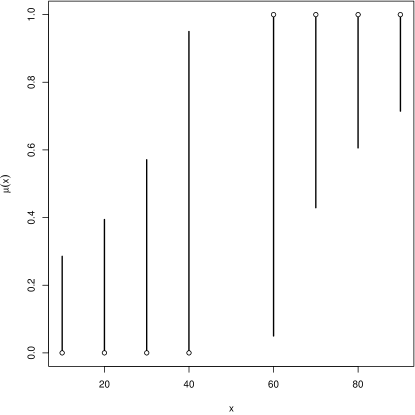
For an exponential family, the submodel canonical statistic is , where is the model matrix. The left panel of Figure 1 shows the observed value of the canonical statistic vector and the support (all possible values) of this vector. As is obvious from the figure, the observed value of the canonical statistic is on the boundary of the convex support, in which case the MLE does not exist in the traditional sense. In this example, the MLE in the completion corresponds to a completely degenerate distribution. This MLE distribution says no data other than what was observed could have been observed. But the sample is not the population and estimates are not parameters. Therefore, this degeneracy is not a problem. To illustrate the uncertainty of estimation, we show confidence intervals (necessarily one-sided) for the saturated model mean value parameters. These one-sided confidence intervals are obtained from functionality in the accompanying glmdr package.
The right panel of Figure 1 shows that, as would be expected from so little data, the confidence intervals are very wide. The MLE in the completion says the probability of observing a response equal to one jumps from zero to one somewhere between 40 and 60. The confidence intervals show that we are fairly sure that this probability goes from near zero at to near one at but we are very unsure where jumps are if there are any. We discuss how these intervals are constructed in Section 4.3. The idea is to first find all canonical parameter values such that the probability of observing the realized degenerate data is greater than some testing level . We then map those canonical parameter values to the mean value parameterization. The degeneracy follows from the estimated Fisher information matrix (for the saturated model canonical parameter vector, also called the linear predictor) at the MLE being singular which it is within the accuracy of computer arithmetic. In this motivating example, the Fisher information matrix is the zero matrix. In this case the MLE of all the saturated model mean value parameters agree with the observed data; they are on the boundary of the set of possible values, either zero or one.
In other examples, such as examples 5.2 and 5.3 below, the MLE distribution is only partially but not completely degenerate. This follows from the estimated Fisher information matrix being singular (to within the accuracy of computer arithmetic) but not the zero matrix. The MLE distribution constrains some components of the response vector to be equal to their observed values, but not all of them. The remaining unconstrained components can be estimated using traditional methods. This is explained in Sections 4.2.
The methodology that we develop is applicable for any discrete regular full exponential family where the MLE does not exist in the traditional sense. We redo Example 2.3 of Geyer (2009) in Section 5.2 using the methodology developed here, and we find that our methodology produces the inferences in that paper in a fraction of the time. We also provide an analysis on a big data set (too large for the methods of Geyer (2009) to run in an acceptable amount of time) to show the (relative) quickness of our implementation.
3 Standard exponential families
Let be a positive Borel measure on a finite-dimensional vector space . The log Laplace transform of is the function defined by
| (1) |
where is the dual space of , where is the canonical bilinear form placing and in duality, and where is the extended real number system, which adds the values and to the real numbers with the obvious extensions to the arithmetic and topology (Rockafellar and Wets, 1998, Section 1.E).
If one prefers, one can take for some , and define
but the coordinate-free view of vector spaces offers more generality and more elegance. Also, as we are about to see, if is the sample space of a standard exponential family, then a subset of is the canonical parameter space, and the distinction between and helps remind us that we should not consider these two spaces to be the same space.
A log Laplace transform is a lower semicontinuous convex function that nowhere takes the value (the value is allowed and occurs where the integral in (1) does not exist) (Geyer, 1990, Theorem 2.1). The effective domain of an extended-real-valued convex function on is
For every , the function defined by
| (2) |
is a probability density with respect to . The set where is any nonempty subset of , is called a standard exponential family of densities with respect to . This family is full if . We also say is the standard exponential family generated by having canonical parameter space , and is the generating measure of . The log likelihood of this family having densities (2) is
| (3) |
A general exponential family (Geyer, 1990, Chapter 1) is a family of probability distributions having a sufficient statistic taking values in a finite-dimensional vector space that induces a family of distributions on that have a standard exponential family of densities with respect to some generating measure. Reduction by sufficiency loses no statistical information, so the theory of standard exponential families tells us everything about general exponential families (Geyer, 1990, Section 1.2).
In the context of general exponential families is called the canonical statistic and the canonical parameter (the terms natural statistic and natural parameter are also used). The set is the canonical parameter space of the family, the set is the canonical parameter space of the full family having the same generating measure. A full exponential family is said to be regular if its canonical parameter space is an open subset of .
4 Calculating the MLE in the completion
We first define the completion of the exponential family.
Definition 1.
Let , , be a sequence of canonical parameter vectors for a standard exponential family having log likelihood (3). Let , and suppose that pointwise as where limits and are allowed. The limiting functions form the closure of the exponential family.
In the above definition is a sequence of affine functions and the limiting function is a generalized affine function. Generalized affine functions and their properties are defined and discussed in Section 6.1.
4.1 Assumptions
So far everything has been for general exponential families. Our implementation requires that the conditions of Brown (1986) hold, and those conditions hold for logistic and log-linear models for categorical data analysis. Now, we restrict our attention to discrete GLMs. This, in effect, includes log-linear models for contingency tables because we can always assume Poisson sampling, which makes them equivalent to multinomial sampling [Agresti, 2013, Section 8.6.7; Geyer, 2009, Section 3.17].
The conditions of Brown that are required for our theory to hold are from Brown (1986, pp. 193–197). These conditions are:
-
(i)
The support of the exponential family is a countable set .
-
(ii)
The exponential family is regular.
-
(iii)
Every is contained in the relative interior of an exposed face of the convex support .
-
(iv)
The convex support of the measure equals , where is the generating measure for the exponential family and is the restriction of to the exposed face .
We let be a likelihood maximizing sequence of canonical parameter vectors, that is,
| (4) |
where the log likelihood is given by (3), is the canonical parameter space of the family, and . Define as in Definition 4. The limiting density corresponds to the MLE distribution in the completion. The mathematical properties of generalized affine functions and this completion construction are studied in Section 6.
4.2 The form of the MLE in the completion
Suppose we know the affine support of the MLE distribution in the completion. This is the smallest affine set (translate of a vector subspace) that contains the canonical statistic with probability one. Denote the affine support by . Since the observed value of the canonical statistic is contained in with probability one, and the canonical statistic for a GLM is , where is the model matrix, is the response vector, and its observed value, we have for some vector space .
Then the limiting conditional model (LCM) in which the MLE in the completion is found is the original model (OM) conditioned on the event
(Geyer, 1990, Theorem 4.3). Suppose we characterize as the subspace where a finite set of linear equalities are satisfied
Then the LCM is the OM conditioned on the event
From this we see that the vectors , span the null space of the Fisher information matrix for the LCM. We collect this in the definition below.
Definition 2.
Let be the -dimensional vector with iid entries from a discrete regular full exponential family. Let be a known model matrix and let be the dimension of the null space of Fisher information. Then the limiting conditional model (LCM) is the original model conditioned on the event
| (5) |
where is the observed value of the response vector and , spans the null space of the Fisher information matrix.
The event (5) fixes some components of the response vector at their observed values and leaves the rest entirely unconstrained. Those components, that are entirely unconstrained are those for which the corresponding components of is zero (or, taking account of the inexactness of computer arithmetic, nearly zero) for all , .
Our theory states that the null space of the Fisher information matrix for the LCM is well approximated by the Fisher information matrix for the OM at parameter values that are close to maximizing the likelihood, see Section 6.4. The vector subspace spanned by the vectors , is called the constancy space of the LCM (Geyer, 2009).
4.3 Calculating one-sided confidence intervals for mean value parameters
We provide a new method for calculating these one-sided confidence intervals that has not been previously published, but whose concept is found in Geyer (2009) in the penultimate paragraph of Section 3.16.2. Let denote the index set of the components of the response vector on which we condition the OM to get the LCM, and let and denote these components considered as a random vector and as an observed value, respectively. Let denote the saturated model canonical parameter (usually called “linear predictor” in GLM theory) with being the submodel canonical parameter vector. Then endpoints for a confidence interval for a scalar parameter are
| (6) |
where is an MLE of the submodel canonical parameter vector in the LCM and is the null space of the Fisher information matrix. At least one of (6) is at the end of the range of this parameter (otherwise we can use conventional two-sided intervals). Steps for obtaining inferences are outlined in Algorithm 1.
For logistic and binomial regression, let denote the mean value parameter vector (here operates componentwise). Then, where the are the binomial sample sizes. In logistic regression we have for all , but in binomial regression we have for all . We could take the confidence interval problem to be
| (7) |
where is taken to be the function of described above, and this can be done for any . The optimization problem in (7) will be more computational stable written as
| (8) |
since can be used to avoid overflow and underflow. More details are included in Section F.3.1 of the Appendix.
For Poisson sampling, let denote the mean value parameter (here operates componentwise like the R function of the same name does), then We take the confidence interval problem to be
| (9) |
where is taken to be the function of described in (6). The optimization in (9) can be done for any . The inference function in the R package glmdr determines one-sided confidence intervals for mean value parameters corresponding to response values for logistic and binomial regression as in (8) and Poisson regression as in (9).
5 Examples
5.1 Complete separation example
We return to the motivating example of Section 2. Here we see that the Fisher information matrix has only null eigenvectors. Thus the LCM is completely degenerate at the one point set containing only the observed value of the canonical statistic of this exponential family. One-sided confidence intervals for mean value parameters (success probability considered as a function of the predictor ) are computed as in Section 4.3. The right panel of Figure 1 in Section 2 displays these one-sided intervals.
This example is reproduced in Section F of the Appendix. The functionality in glmdr was used to calculate the one-sided confidence intervals for mean value parameters (inference function) and determine that the LCM is completely degenerate (glmdr function).
5.2 Example in Section 2.3 of Geyer (2009)
This example consists of a contingency table with seven dimensions hence cells. These data now have a permanent location(Eck and Geyer, ). There is one response variable that gives the cell counts and seven categorical predictors , , that specify the cells of the contingency table. We fit a generalized linear regression model where is taken to be Poisson distributed. We consider a model with all three-way interactions included but no higher-order terms. The software in the glmdr package reproduces the original analysis, as seen throughout the Appendix. The inference function computed the one-sided confidence intervals for mean value parameters that are on the boundary of their support, in this case equal to zero. The results are depicted in Table 1, this table is the same as Table 2 in Geyer (2009) and it is reproduced in Section J of the Appendix.
| lower | upper | |||||||
|---|---|---|---|---|---|---|---|---|
| 0 | 0 | 0 | 0 | 0 | 0 | 0 | 0 | 0.28631 |
| 0 | 0 | 0 | 1 | 0 | 0 | 0 | 0 | 0.14083 |
| 1 | 1 | 0 | 0 | 1 | 0 | 0 | 0 | 0.21997 |
| 1 | 1 | 0 | 1 | 1 | 0 | 0 | 0 | 0.42096 |
| 0 | 0 | 0 | 0 | 0 | 1 | 0 | 0 | 0.08946 |
| 0 | 0 | 0 | 1 | 0 | 1 | 0 | 0 | 0.09377 |
| 1 | 1 | 0 | 0 | 1 | 1 | 0 | 0 | 0.19302 |
| 1 | 1 | 0 | 1 | 1 | 1 | 0 | 0 | 0.28870 |
| 0 | 0 | 0 | 0 | 0 | 0 | 1 | 0 | 0.10631 |
| 0 | 0 | 0 | 1 | 0 | 0 | 1 | 0 | 0.11415 |
| 1 | 1 | 0 | 0 | 1 | 0 | 1 | 0 | 0.09129 |
| 1 | 1 | 0 | 1 | 1 | 0 | 1 | 0 | 0.26461 |
| 0 | 0 | 0 | 0 | 0 | 1 | 1 | 0 | 0.06669 |
| 0 | 0 | 0 | 1 | 0 | 1 | 1 | 0 | 0.15478 |
| 1 | 1 | 0 | 0 | 1 | 1 | 1 | 0 | 0.14097 |
| 1 | 1 | 0 | 1 | 1 | 1 | 1 | 0 | 0.32392 |
The only material difference between our implementation and the linear programming in Geyer (2009) is computational time. Our implementation provided one-sided confidence intervals for those responses that are on the boundary of their support in 1.253 seconds, while the functions in the rcdd package take 4.84 seconds of computer time. This is a big difference for a relatively small amount of data. Inference for the MLE in the LCM are included in Section K of the Appendix.
5.3 Big data example
This example uses the other dataset at (Eck and Geyer, ). It shows our methods are much faster than the linear programming method of Geyer (2009). The functionality in the glmdr determined the LCM and computed one-sided confidence intervals for mean value parameters that are on the boundary of their support in about a minute. The same task using the rcdd package took 3 days, 4 hours, 0 minutes, and 40.937 seconds. (This was on oak.stat.umn.edu, which is an Intel(R) Core(TM) i7-6700 CPU @ 3.40GHz.) Both methods yielded the same conclusions.
This dataset consists of five categorical variables with four levels each and a response variable that is Poisson distributed. A model with all four-way interaction terms is fit to this data. It may seem that the four way interaction model is too large (1024 data points vs 781 parameters) but tests select this model over simpler models, see Table 2.
| null model | alternative model | df | Deviance | Pr() |
|---|---|---|---|---|
| m1 | m4 | 765 | 904.8 | 0.00034 |
| m2 | m4 | 675 | 799.2 | 0.00066 |
| m3 | m4 | 405 | 534.4 | 0.00002 |
One-sided 95% confidence intervals for mean valued parameters whose MLE is equal to zero are displayed in Table 3. The full table is included in Section K.5 of the Appendix. Some of the intervals in Table 3 are relatively wide, this represents non-trivial uncertainty about the observed MLE being zero. This example is completely reproduced in Section K of the Appendix.
| X1 | X2 | X3 | X4 | X5 | lower bound | upper bound |
|---|---|---|---|---|---|---|
| a | a | b | a | a | 0 | 0.1695 |
| a | b | b | a | a | 0 | 0.1354 |
| a | c | b | a | a | 0 | 0.2292 |
| a | d | b | a | a | 0 | 2.4616 |
| d | d | c | a | a | 0 | 0.0002 |
| a | c | d | a | a | 0 | 0.0133 |
6 Mathematical details
In this Section we provide the mathematical justification for our inferential procedure. We develop the theory of generalized affine functions (Geyer, 1990) and then show that this theory, combined with conditions for the exponential family closure of Brown (1986), facilitates the convergence of moments of all orders along a sequence of maximum likelihood iterates. We close this Section by establishing that our mathematical technique can estimate the correct null space of the Fisher information matrix, and this allows for valid statistical inference when the MLE does not exist in the conventional sense.
6.1 Generalized affine functions
6.1.1 Characterization on affine spaces
Exponential families defined on affine spaces instead of vector spaces are in many ways more elegant (Geyer, 1990, Sections 1.4 and 1.5 and Chapter 4). To start, a family of densities with respect to a positive Borel measure on an affine space is a standard exponential family if the log densities are affine functions. We complete the exponential family by taking pointwise limits of densities, allowing and as limits (Geyer, 1990, Chapter 4).
We call these limits generalized affine functions. Real-valued affine functions on an affine space are functions that are are both convex and concave. Generalized affine functions on an affine space are extended-real-valued functions that are are both concave and convex (Geyer, 1990, Chapter 4). (For a definition of extended-real-valued convex functions see Rockafellar (1970, Chapter 4).)
We thus have two characterizations of generalized affine functions: functions that are both convex and concave and functions that are limits of sequences of affine functions. Further characterizations will be given below.
Let denote a sequence of affine functions that are log densities in a standard exponential family with respect to , that is, for all . Since pointwise if and only if pointwise, the idea of completing an exponential family naturally leads to the study of generalized affine functions.
If is a generalized affine function, we use the notation
Theorem 1.
An extended-real-valued function on a finite-dimensional affine space is generalized affine if and only if one of the following cases holds
-
(a)
,
-
(b)
,
-
(c)
and is an affine function, or
-
(d)
there is a hyperplane such that for all points on one side of , for all points on the other side of , and restricted to is a generalized affine function.
All theorems for which a proof does not follow the theorem statement are proved in Sections A-C in the Appendix. The intention is that this theorem is applied recursively. If we are in case (d), then the restriction of to is another generalized affine function to which the theorem applies. Since a nested sequence of hyperplanes can have length at most the dimension of , the recursion always terminates.
6.1.2 Topology
Let denote the space of generalized affine functions on a finite-dimensional affine space with the topology of pointwise convergence.
Theorem 2.
is a compact Hausdorff space.
Theorem 3.
is a first countable topological space.
Corollary 1.
is sequentially compact.
Sequentially compact means every sequence has a (pointwise) convergent subsequence. That this follows from the two preceding theorems is well known (Steen and Seebach, 1978, p. 22, gives a proof). The space is not metrizable, unless is zero-dimensional (Geyer, 1990, penultimate paragraph of Section 3.3). So we cannot use - arguments, but we can use arguments involving sequences, using sequential compactness.
Let be a positive Borel measure on , and let be a nonempty subset of such that
| (10) |
We call a standard generalized exponential family of log densities with respect to . Let denote the closure of in .
Theorem 4.
Maximum likelihood estimates always exist in the closure .
Proof.
Suppose is the observed value of the canonical statistic. Then there exists a sequence in such that
This sequence has a convergent subsequence in . This limit is in and maximizes the likelihood. ∎
For full exponential families or even closed convex exponential families the closure only contains proper log probability densities ( that satisfy the equation in (10)). This is shown by Geyer (1990, Chapter 2) and also by Csiszár and Matúš (2005). We claim that the closure is the right way to think about completion of the exponential families, as it is explicitly constructed to facilitate useful statistical inference for practitioners. For curved exponential families and for general non-full exponential families, applying Fatou’s lemma to pointwise convergence in gives only
| (11) |
When the integral in (11) is strictly less than one we say is an improper log probability density. Examples in Geyer (1990, Chapter 4) show that improper probability densities cannot be avoided in curved exponential families.
Geyer (1990, Theorem 4.3) shows that this closure of an exponential family can be thought of as a union of exponential families, so this generalizes the notion in Brown (1986) of the closure as an aggregate exponential family. Thus our method generalizes all previous methods of completing exponential families. Admittedly, this characterization of the completion of an exponential family is very different from any other in its ignoring of parameters. Only log densities appear. Unless one wants to call them parameters — and that conflicts with the usual definition of parameters as real-valued — parameters just do not appear. So in the next section, we bring parameters back.
6.1.3 Characterization on vector spaces
In this section we take sample space to be vector space (which, of course, is also an affine space, so the results of the preceding section continue to hold). Recall from Section 3 above, that denotes the dual space of , which contains the canonical parameter space of the exponential family.
Theorem 5.
An extended-real-valued function on a finite-dimensional vector space is generalized affine if and only if there exist finite sequences (perhaps of length zero) of vectors , in in and scalars , such that , are linearly independent and has the following form. Define and, inductively, for integers such that
all of these sets (if any) being nonempty. Then whenever for any , whenever for any , and is either affine or constant on , where and are allowed for constant values.
The “if any” refers to the case where the sequences have length zero, in which case the theorem asserts that is affine on or constant on . As we saw in the preceding section, we are interested in likelihood maximizing sequences. Here we represent the likelihood maximizing sequence in the coordinates of the linearly independent vectors that characterize the generalized affine function according to its Theorem 5 representation. Let be a likelihood maximizing sequence of canonical parameter vectors as in (4). To make connection with the preceding section, define Then is a sequence of affine functions, which has a subsequence that converges (in ) to some generalized affine function , which maximizes the likelihood:
| (12) |
The following lemma gives us a better understanding of the convergence .
Lemma 1.
Suppose that a generalized affine function on a finite dimensional vector space is finite at at least one point. Represent as in Theorem 5, and extend , to be a basis , for . Suppose is a sequence of affine functions converging to in . Then there are sequences of scalars and such that
| (13) |
and, as , we have
-
(a)
, for ,
-
(b)
, for ,
-
(c)
converges, for , and
-
(d)
converges.
In (13) the first sum is empty when and the second sum is empty when . Such empty sums are zero by convention. The results given in Lemma 1 are applicable to generalized affine functions in full generality. The case of interest to us, however, is when is the likelihood maximizing sequence constructed above.
Corollary 2.
For data from a regular full exponential family defined on a vector space , suppose is a likelihood maximizing sequence satisfying (4) with log densities defined by (12) converging pointwise to a generalized affine function . Characterize and as in Theorem 5 and Lemma 1. Define . Then conclusions (a) and (b) of Lemma 1 hold in this setting and
where is the MLE of the exponential family conditioned on the event .
In case the conclusion is the trivial zero converges to zero. The original exponential family conditioned on the event is what Geyer (2009) calls the LCM.
Proof.
6.2 Convergence theorems
6.2.1 Cumulant generating function convergence
The CGF of the distribution of the canonical statistic for parameter value is the function defined by
| (14) |
provided this distribution has a CGF, which it does if and only if is finite on a neighborhood of zero, that is, if and only if . Thus every distribution in a full exponential family has a CGF if and only if the family is regular. Derivatives of evaluated at zero are the cumulants of the distribution for . These are the same as derivatives of evaluated at .
We now show CGF convergence along likelihood maximizing sequences (4). This implies convergence in distribution and convergence of moments of all orders. Theorems 6 and 7 in this section say when CGF convergence occurs. Their conditions are somewhat unnatural (especially those of Theorem 6). However, the counterexample in Section D of the Appendix shows not only that some conditions are necessary to obtain CGF convergence (it does not occur for all full discrete exponential families) but also that the conditions of Theorem 6 are sharp, being just what is needed to rule out that example.
The CGF of the distribution having log density that is the generalized affine function is defined by
and similarly
where we assume are the log densities for a likelihood maximizing sequence such that pointwise. The next theorem characterizes when pointwise.
Let denote the log Laplace transform of the restriction of to the set , that is,
where, as usual, the value of the integral is taken to be when the integral does not exist (a convention that will hold for the rest of this section).
Theorem 6.
Let be a finite-dimensional vector space of dimension . For data from a regular full exponential family with natural parameter space and generating measure , assume that every distribution in the family has a cumulant generating function. Suppose that is a likelihood maximizing sequence satisfying (4) with log densities converging pointwise to a generalized affine function . Characterize as in Theorem 5. When , and for , define
| (15) |
and assume that
| (16) |
Then converges to pointwise for all in a neighborhood of 0.
Remarks:
-
1.
The quantities in (15) and (16) are technical in nature and are an artifact of the proof technique. Without these conditions, there exists circumstances in which CGF convergence fails to hold. The next remarks elaborate these quantities. The next Theorem shows that (16) is satisfied under the more intuitive conditions of Brown (1986).
-
2.
The sets , arise from the characterization of a generalized affine function given in Theorem 5 which is a pointwise limit of the densities of log densities . The assumption that the exponential family is discrete and full implies that (Geyer, 1990, Theorem 2.7) which in turn implies that for all ,,. We now focus on sets of points such that . The first iteration of the recursive structure in the Theorem 5 characterization of a generalized affine function gives . Now consider a point , it is possible in a full regular discrete exponential family for , where the pair form the hyperplane . Such points form the set , and the sets , , are similarly motivated. Our proof technique requires bounding of the CGF restricted to evaluated along by the quantities in (16), see (26) in the proof of Theorem 6.
-
3.
The conditions in (16) rule out pathological examples for which CGF convergence does not hold. In Section D of the Appendix we provide an example for which (16) does not hold and a lack of CGF convergence follows. Moreover, this example demonstrates a lack of convergence of second moments and our approach for statistical inference fails as a result. More general closures of exponential families in Csiszár and Matúš (2005, 2008) and Geyer (1990, unpublished PhD thesis, Chapter 4) do not assume condition (16) and therefore rule out CGF convergence in full generality.
-
4.
Discrete exponential families automatically satisfy (16) when the generating measure satisfies
In this setting, corresponds to the probability mass function for the random variable conditional on the occurrence of . Thus,Therefore, Theorem 6 is applicable for the non-existence of the maximum likelihood estimator that may arise in logistic and multinomial regression or any exponential family with finite support. The same is not necessarily so for Poisson regression. The next Theorem provides CGF convergence for Poisson sampling under the regularity conditions of Brown (1986).
We show in the next theorem that discrete families with convex polyhedral support also satisfy (16) under additional regularity conditions that hold in practical applications. When is convex polyhedron, we can write as in (Rockafellar and Wets, 1998, Theorem 6.46). When the MLE does not exist, the data is on the boundary of . Denote the active set of indices corresponding to the boundary containing by In preparation for Theorem 7 we define the normal cone , the tangent cone , and faces of convex sets and then state conditions required on .
Definition 3.
The normal cone of a convex set in the finite dimensional vector space at a point is
Definition 4.
The tangent cone of a convex set in the finite dimensional vector space at a point is
where denotes the set closure operation.
When is a convex polyhedron, and are both convex polyhedron with formulas given in (Rockafellar and Wets, 1998, Theorem 6.46). These formulas are
Definition 5.
A face of a convex set is a convex subset of such that every (closed) line segment in with a relative interior point in has both endpoints in . An exposed face of is a face where a certain linear function achieves its maximum over (Rockafellar, 1970, p. 162).
The four conditions of Brown, stated in Section 4.1 are required for the Theorem to hold. Conditions (i) and (ii) are already assumed in Theorem 6. It is now shown that discrete exponential families satisfy (16) under the above conditions.
Theorem 7.
Assume the conditions of Theorem 6 with the omission of (16) when . Let denote the convex support of the exponential family. Assume that the exponential family satisfies the conditions of Brown:
-
(i)
The support of the exponential family is a countable set .
-
(ii)
The exponential family is regular.
-
(iii)
Every is contained in the relative interior of an exposed face of the convex support .
-
(iv)
The convex support of the measure equals , where is the generating measure for the exponential family.
Then (16) holds and we have that converges to pointwise for all in a neighborhood of zero.
6.3 Extensions of CGF convergence
Theorems 6 and 7 both verify CGF convergence along likelihood maximizing sequences (4) on neighborhoods of zero. The next theorems show that CGF convergence on neighborhoods of zero is enough to imply convergence in distribution and of moments of all orders. Therefore moments of distributions with log densities that are affine functions converge along likelihood maximizing sequences (4) to those of a limiting distributions whose log density is a generalized affine function.
Suppose that is a random vector in a finite-dimensional vector space having a moment generating function (MGF) , then for , regardless of whether the MGF exist or not. It follows that the MGF of for all determine the MGF of and vice versa, when these MGF exist. More generally,
| (17) |
This observation applied to characteristic functions rather than MGF is called the Cramér-Wold theorem. In that context it is more trivial because characteristic functions always exist.
If , is a basis for a vector space , then Halmos (1974, Theorem 2 of Section 15) states that there exists a unique dual basis , for that satisfies
| (18) |
Theorem 8.
If is a random vector in having an MGF, then the random scalar has an MGF for all . Conversely, if has an MGF for all , then has an MGF.
Theorem 9.
Suppose , , , is a sequence of random vectors, and suppose their moment generating functions converge pointwise on a neighborhood of zero. Then
| (19) |
and has an MGF , and , for .
Theorem 10.
Under the assumptions of Theorem 9, suppose , , are vectors defined on , the dual space of . Then is uniformly integrable so
The combination of Theorems 6-10 provide a methodology for statistical inference along likelihood maximizing sequences when the MLE is in the completion of the exponential family. In particular, we have convergence in distribution and convergence of moments of all orders along likelihood maximizing sequence. The limiting distribution in this context is a generalized exponential family with density where is a generalized affine function.
6.4 Convergence of null spaces of Fisher information
Our implementation for finding the MLE in the completion relies on finding the null space of Fisher information matrix. We first define an appropriate notion of convergence of vector subspaces, and then prove that the null spaces corresponding to a sequence of semidefinite matrices converge.
Definition 6.
Painlevé-Kuratowski set convergence (Rockafellar and Wets, 1998, Section 4.A) can be defined as follows (Rockafellar and Wets (1998) give many equivalent characterizations). If is a sequence of sets in and is another set in , then we say if
-
(i)
For every there exists a subsequence of the natural numbers and there exist such that .
-
(ii)
For every sequence in such that there exists a natural number such that whenever , we have .
Theorem 11.
Suppose that is a sequence of positive semidefinite matrices and componentwise. Fix less than half of the least nonzero eigenvalue of unless is the zero matrix in which case may be chosen arbitrarily. Let denote the subspace spanned by the eigenvectors of corresponding to eigenvalues that are less than . Let denote the null space of . Then (Painlevé-Kuratowski).
In our context, the sequence of matrices in Theorem 11 correspond to the Fisher information matrices obtained from a discrete exponential family whose canonical parameters are substituted for those in a likelihood maximizing sequence.
Supplementary Materials
The R package glmdr accompanies this submission (Geyer and Eck, 2016).
7 Discussion
TThe theory of generalized affine functions and the geometry of exponential families allow GLM software to provide fast and scalable maximum likelihood estimation when the observed value of the canonical statistic is on the boundary of its support. The limiting probability distribution evaluated along the iterates of a likelihood maximizing sequence has log density that is a generalized affine function with structure given by Theorem 5. Cumulant generating functions converge along this sequence of iterates (Theorems 6 and 7), as do estimates of moments of all orders (Theorem 10), and so do the null spaces of Fisher information matrices (Theorem 11). These results allow one to obtain the MLE in the completion of the exponential family and to construct one-sided confidence intervals for mean value parameters that are on the boundary of their support.
The glmdr package computes one-sided confidence intervals for mean value parameters that are on the boundary of their support. Parameter estimation in the LCM is conducted in the traditional manner. The costs of computing the support of a LCM using the glmdr package are minimal compared to the repeated linear programming in the rcdd package. It is much faster to let optimization software, such as glm in R, simply go uphill on the log likelihood of the exponential family until a convergence tolerance is reached, determine null eigenvectors of the limiting Fisher information matrix, and then compute one-sided confidence intervals than it is to compute the necessary repeated linear programming to achieve the same inferences. Our examples demonstrate that massive time savings are possible using our methodology.
The chance of observing a canonical statistic on the boundary of its support increases when the dimension of the model increases. Researchers naturally want to include all possibly relevant covariates in an analysis, and this will often result in the MLE not existing in the conventional sense. Our methods provide a computationally inexpensive solution to this problem.
Acknowledgements
We would like to thank Forrest W. Crawford, his comments led to an improved and more interesting version of this paper.
Appendix
Appendix A Proofs of main results
Proof of Theorem 6.
First consider the case when , the sequences of vectors and scalars are both of length zero. There are no sets and in this setting and is affine on . From Lemma 1 we have . From Corollary 2, as . We observe that from continuity of the cumulant function. The existence of the MLE in this setting implies that there is a neighborhood about 0 denoted by such that . Pick and observe that . Therefore when .
Now consider the case when . Define for all . In this scenario we have
From (Geyer, 1990, Theorem 2.2), we know that
| (20) |
as since for all . The left hand side of both convergence arrows in (20) are convex functions of and the right hand side is a proper convex function. If is nonempty, which holds whenever is nonempty, then the convergence in (20) is uniform on compact subsets of (Rockafellar and Wets, 1998, Theorem 7.17). Also (Rockafellar and Wets, 1998, Theorem 7.14), uniform convergence on compact sets is the same as continuous convergence. Using continuous convergence, we have that both
where as by Lemma 1. Thus
This concludes the proof when .
For the rest of the proof we will assume that where dim() = . Represent the sequence in coordinate form as with scalars , . For , we know that as from Corollary 2. The existence of the MLE in this setting implies that there is a neighborhood about 0, denoted by , such that . Pick , fix , and construct -boxes about and , denoted by and respectively, such that both . Let be the set of vertices of . For all define
| (21) |
From the conclusions of Lemma 1 and Corollary 2, we can pick an integer such that and for all and . For all , we have
| (22) |
for all . The integrability of and follows from
Therefore,
which implies that
| (23) |
by dominated convergence. To complete the proof, we need to verify that
| (24) |
We know that (24) holds when in (16) because of (23). Now suppose that . We have,
| (25) |
and
| (26) |
for all by the assumption given by (16). The assumption that the exponential family is discrete and full implies that (Geyer, 1990, Theorem 2.7). This in turn implies that for all which then implies that Putting (22), (25), and (26) together we can conclude that (24) holds as by dominated convergence and
| (27) |
for all , where the last equality is . This verifies CGF convergence on neighborhoods of 0. ∎
Proof of Theorem 7.
Represent as in Theorem 5. Denote the normal cone of the convex polyhedron support at the data by . We show that a sequence of scalars and a linearly independent set of vectors can be chosen so that , and
| (28) |
for where so that (16) holds. We will prove this by induction with the hypothesis , , that (28) holds for where the vectors .
We first verify the basis of the induction. The assumption that the exponential family is discrete and full implies that (Geyer, 1990, Theorem 2.7). This in turn implies that for all . This then implies that Thus and the base of the induction holds with and .
We now show that follows from for . We first establish that is an exposed face of . This is needed so that (28) holds for . Let be the collection of closed line segments with endpoints in . Arbitrarily choose such that an interior point and . We can write , , where and are the endpoints of . Since by construction, we have that and because by . Now,
and
Therefore and this verifies that is a face of since was chosen arbitrarily. The function defined on , is maximized over . Therefore is an exposed face of by definition. The exposed face since and the convex support of the measure is by assumption. Thus, .
The sets and are both convex and are therefore regular at every point (Rockafellar and Wets, 1998, Theorem 6.20). We can write since and are convex sets that cannot be separated where + denotes Minkowski addition in this case (Rockafellar and Wets, 1998, Theorem 6.42). The normal cone has the form
Therefore, we can write
| (29) |
where and , . For , we have that
Let . We can therefore write
and
| (30) |
A similar argument to that of (30) verifies that
This confirms that (28) holds for and this establishes that follows from .
Proof of Theorem 11.
We first consider the case that is positive definite and . We can write where is a perturbation of for large . From Weyl’s inequality (Weyl, 1912), we have that all eigenvalues of are bounded above zero for large and as a result. Therefore, as when is positive definite.
Now consider the case that is not strictly positive definite. Without loss of generality, let be a unit vector. For all , let denote the subspace spanned by the eigenvectors of corresponding to eigenvalues that are less than . By construction, .
From (Rockafellar and Wets, 1998, Example 10.28), if has zero eigenvalues, then for sufficiently large there are exactly eigenvalues of are less than and eigenvalues of greater than for all . The same is true with respect to for all greater than . Thus which implies that for all .
We now verify part (i) of Painlevé-Kuratowski set convergence with respect to . Let be such that for all . Let and be the eigenvalues and eigenvectors of , with the eigenvalues listed in decreasing orders. Without loss of generality, we assume that the eigenvectors are orthonormal. Then, , , and . There have to be eigenvectors such that with corresponding eigenvalues that are very small since . But conversely, any eigenvalues such that must have
Define and where by construction. Now,
for all . Therefore, for every , there exists a sequence such that since this argument holds for all . This establishes part (i) of Painlevé-Kuratowski set convergence.
We now show part (ii) of Painlevé-Kuratowski set convergence. Suppose that and there exists a natural number such that whenever , and we will establish that . From hypothesis, we have that . Without loss of generality, we assume that is a unit vector and that for all . From the assumption that we have
| (31) |
for all . The reverse triangle inequality gives
and (31) implies for all . Since this argument holds for all , we have that . This establishes part (ii) of Painlevé-Kuratowski convergence with respect to . Thus . ∎
Appendix B Proofs of the properties of generalized affine functions
We first prove Theorem 2.
Proof.
Let denote the space of all functions with the topology of pointwise convergence. This makes , an infinite product. Then is compact by Tychonoff’s theorem. We now show that is closed in hence compact.
Let be any point in the closure of . Then there is a net in that converges to . For any and in such that and and any , write .
Then
whenever the right hand side makes sense (is not ), which happens eventually, since and both converge to limits that are not . Hence
and is convex. By symmetry it is also concave and hence is generalized affine. Thus contains its closure and is closed.
is Hausdorff because the product of Hausdorff spaces is Hausdorff. is Hausdorff because subspaces of Hausdorff spaces are Hausdorff. ∎
In order to prove Theorem 1, an intermediate Theorem is first stated and its proof is provided.
Theorem 12.
An extended-real-valued function on a finite-dimensional affine space is generalized affine if and only if and are convex sets, is an affine set, and is affine on .
Proof.
To simplify notation, define
| (32a) | ||||
| (32b) | ||||
| (32c) | ||||
First assume is generalized affine. Then is convex because is convex, and is convex because is concave. For any two distinct points and any , The points , , and lie on a straight line. The convexity and concavity inequalities together imply
It follows that is an affine set and restricted to is an affine function.
Conversely, assume and are convex sets, is an affine set, and is affine on . We must show that is convex and concave. We just prove convexity because the other proof just the same proof applied to . So consider two distinct points and (the convexity inequality is vacuous when either of or is in ). Write .
If and are both in , then being an affine set implies and the convexity inequality involving , , and follows from being affine on . If and are both in , then being a convex set implies and the convexity inequality involving , , and follows from .
The only case remaining is and . In this case, there can be no other point on the line determined by and that is in , because is an affine set. Hence all the points in this line on one side of must be in and all the points on the other side must be in . Thus , and the convexity inequality involving , , and follows from . ∎
We now provide the proof of Theorem 1.
Proof.
Again we use the notation in (32a), (32b), and (32c). First we show that all four cases define generalized affine functions. The first three cases obviously satisfy the conditions of Theorem 12.
In case (d), we just prove convexity because the other proof just the same proof applied to .
If and are both in , then being generalized affine on implies the convexity inequality for and and any point between them. If and are both in and not both in , say , then any point between and is also not in , and hence is in because it is on the same side of as is. So implies the convexity inequality involving , , and . That completes the proof that all four cases define generalized affine functions.
So we now show that every generalized affine function falls in one of these four cases. Suppose is generalized affine, and assume that we are not in case (a), (b), or (c). Then at least one of and is nonempty. This implies , hence, being an affine set, is dense in . If , then is dense in , hence being a convex set, and we are in case (c) contrary to assumption. Hence . The same proof with and swapped implies .
Hence and are disjoint nonempty convex sets, so by the separating hyperplane theorem (Rockafellar, 1970, Theorem 11.3), there is an affine function on such that
| when | (33a) | |||||
| when | (33b) | |||||
and the hyperplane in question is
Again we know is dense in , hence is dense in the half space on one side of , and is dense in the half space on the other side of . Now convexity of and imply
| when | (34a) | |||||
| when | (34b) | |||||
That is generalized affine on follows from being generalized affine on . Thus we are in case (d). ∎
We now want to show that is first countable. In aid of that we first prove a lemma.
Lemma 2.
Every finite-dimensional affine space is second countable and metrizable. If is a countable dense set in , then every point of is contained in the interior of the convex hull of some finite subset of . The same is true of any open convex subset of : every point of is contained in the interior of the convex hull of some finite subset of .
Proof.
The first assertion is trivial. If the dimension of is , then the topology of is defined to make any invertible affine function a homeomorphism.
The second assertion is just the case of the third assertion.
Assume to get a contradiction that the third assertion is false. Then there is a point that is disjoint from the convex hull of . It follows that there is a strongly separating hyperplane (Rockafellar, 1970, Corollary 11.4.2), hence an affine function such that
But this violates being in . ∎
We can now prove Theorem 3.
Proof.
We need to show there is a countable local base at for any . A set is a neighborhood of if it has the form
| (35) |
where is a finite subset of and each is a neighborhood of in .
We prove first countability by induction on the dimension of using Theorem 1. For the basis of the induction, if , then is homeomorphic to , hence actually second countable.
We now show that there is a countable local base at in each of the four cases of Theorem 1. Fix a countable dense set in (there is one by Lemma 2).
There is only one satisfying case (a), the constant function having the value everywhere. In this case, a general neighborhood (35) contains a neighborhood of the form
where can be an integer. Also by Lemma 2 there exists a finite subset of that contains in the interior of its convex hull. Then, by concavity of elements of , the neighborhood
is contained in . Hence the collection
| (36) |
is a countable local base at .
The proof for case (b) is similar. In case (c) we are considering an affine function on . In this case, a general neighborhood (35) contains a neighborhood of the form
where is a finite subset of and is a positive integer.
Again use Lemma 2 to choose a finite set containing in the interior of its convex hull. Then, by convexity and concavity of elements of , the neighborhood
is contained in because any can be written as a convex combination of the elements of
where the are nonnegative and sum to one, so implies
by the convexity inequality, and the same with the inequalities reversed and replaced by by the concavity inequality. Hence the collection (36) with as defined in this part is a countable local base at .
In case (d) we are considering a generalized affine function that is neither affine nor constant. Then, as the proof of Theorem 1 shows, there is a hyperplane that is the boundary of and . The induction hypothesis is that is first countable, that is, there is a countable family of neighborhoods of in such that
is a countable local base for at the restriction of to .
Again consider a general neighborhood of (35); call it . Let denote the restriction of to . For any subset of let be defined by
Then the induction hypothesis is that there exists a such that is contained in .
Also adopt the notation (32a), (32b), and (32c) used in the proofs of Theorems 12 and 1. By Lemma 2 choose a set in that contains in the interior of its convex hull, and choose a set in that contains in the interior of its convex hull,
Then, by convexity and concavity of elements of , the neighborhood
| (37) |
is contained in . To see this, first consider (if there are any). Any in (37) has because of . Next consider (if there are any). Any in (37) has because of concavity of assures , and we chose so that . Last consider (if there are any). Any in (37) has because of convexity of assures , and we chose so that .
Hence the collection
is a countable local base at .
We forgot the case where is empty. Then is a one-point space whose only element is the empty function (that has no argument-value pairs). It is trivially first countable. ∎
We now prove Theorem 5.
Proof.
First, assume satisfies the conditions of Theorem 1 on . We then show that satisfies the conditions of Theorem 5 by induction on the dimension of . The induction hypothesis, , is that the conclusions of Theorem 1 imply that the conclusions of Theorem 5 hold when dim() = . We now show that holds. In this setting, . Therefore our result holds with and is constant on . The basis of the induction holds.
Let dim() = . We now show that implies that holds. In the event that is characterized by case (a) or (b) of Theorem 1 then our result holds with . If case (c) of Theorem 1 characterizes then there is an affine function defined by , such that for such that , for such that , and is generalized affine on the hyperplane . The hyperplane is -dimensional affine subspace of . Now, for some arbitrary , define
where the last equality follows from . The space is a -dimensional vector subspace of since every affine space containing the origin is a vector subspace (Rockafellar, 1970, Theorem 1.1) and because every translate of an affine space is another affine space (Rockafellar, 1970, pp. 4). Let
| (38) |
The function is convex since the composition of a convex function with an affine function is convex. To see this, let , pick and observe that
A similar argument shows that is concave. Therefore is generalized affine. From our induction hypothesis, the conclusions of Theorem 1 imply that our result holds for the generalized affine function . These conditions are that there exist finite sequences of vectors , , being a linearly independent subset of , the dual space of , and scalars , , such that has the following form. Define and, inductively, for integers such that
| (39) |
all of these sets (if any) being nonempty. Then whenever for any , whenever for any , and is either affine or constant on , where and are allowed for constant values.
It remains to show that the conditions of Theorem 5 hold with respect to . The vectors , can be extended to form a set of vectors , in by the Hahn-Banach Theorem (Rudin, 1991, Theorem 3.6). The vectors , , form a linearly independent subset of . To see this, let on for scalars , . Then on which implies that for by the definition of linearly independent. Let , and, for , define
| (40) |
where for and as a result. We see that whenever . Therefore for all for any . The same derivation shows that whenever for any . The generalized affine function is either affine or constant on , where and are allowed for constant values since the composition of an affine function with an affine function is affine.
We now show that the vectors are linearly independent. Assume that on for scalars , . This assumption implies that on where is the restriction of to . Thus is an element of and on since on . Therefore where for from what has already been shown. In the event that , we can conclude that are linearly independent. Now consider . In this case, implies that where . This states that on . Therefore, for all which implies that is the zero vector, which is a contradiction. Thus and we can conclude that are linearly independent. This completes one direction of the proof.
Now assume that satisfies the conclusions of Theorem 5 and show that these conclusions imply that Theorem 1 holds by induction on . The induction hypothesis, , is that the conclusions of Theorem 5 imply that the conclusions of Theorem 1 hold for sequences of length . For the basis of the induction let . We now show that holds. The generalized affine function is either affine or constant on where and are allowed for constant values. This characterization of is the same as cases (a) of (b) of Theorem 1. The basis of the induction holds.
We now show that implies that holds. When the length of sequences is , there exist vectors and scalars such that has the following form. Define and, inductively, for integers , , such that the sets in (40) are all nonempty. Then whenever for any , whenever for any , and is either affine or constant on , where and are allowed for constant values. From the definition of the sets , , and , there is an affine function defined by , such that for all such that and for all such that . This is equivalent to the case (c) characterization of in Theorem 1, provided we show that the restriction of to is a generalized affine function.
Define for some arbitrary . Let dim() = . The space is a ()-dimensional vector subspace of . Define as in (38). Let be the restriction of to so that is an element of for . Now let and, for , we can define the sets as in (39) where . We see that whenever . Therefore for all for any . The same derivation shows that whenever for any . The generalized affine function is either affine or constant on , where and are allowed for constant values. Therefore meets the conditions of Theorem 5 with sequences of length . From , we know that the conclusions of Theorem 1 hold with respect to . This completes the proof. ∎
We now prove Lemma 1 using the characterization of generalized affine functions on finite-dimensional vector spaces given by Theorem 5.
Proof.
First suppose that converges to . The assumption that is finite at at least one point guarantees that is affine on from Theorem 5. For all we can write where and . The convergence implies that , where the set of s is empty when and that as . Thus conclusions (c) and (d) hold. To show that conclusions (a) and (b) hold we will suppose that , because these conclusions are vacuous when . Both cases (a) and (b) will be shown by induction with the hypothesis that and as for . We now show that the basis of this induction holds. Pick and observe that
since and pointwise. From this, we see that as and as from part (c). Therefore holds. It is now shown that implies that holds. There exists a basis in , the dual space of , such that when and when . The set of vectors is a basis of since . Arbitrarily choose a such that where . At this choice of we see that and
as . Therefore as . Now arbitrarily choose where is defined as before and . At this choice of we see that and
| (41) |
as . It follows from (41) that
for sufficiently large . This implies that
for sufficiently large . From the arbitrariness of the constants and and (41), we can conclude that as . Therefore holds and this completes one direction of the proof.
Appendix C Proofs of MGF and moment convergence results
We first prove Theorem 8.
Proof.
Suppose is an MGF, hence finite on a neighborhood of zero.Fix . Then by (17) is finite whenever . Continuity of scalar multiplication means there exists an such that whenever . That proves one direction.
Conversely, suppose is an MGF for each . Suppose , is a basis for and , is the dual basis for that satisfies (18). Then there exists such that is finite on for each .
We can write each as a linear combination of basis vectors
where the are scalars that are unique (Halmos, 1974, Theorem 1 of Section 15). Applying (18) we get
so
and
Suppose
(the set of all such is a neighborhood of in ). Let denote the sign function, which takes values , , and as its argument is negative, zero, or positive, and write
Then we can write as a convex combination
So, by convexity of the exponential function,
That proves the other direction. ∎
We now prove Theorem 9.
Proof.
The one-dimensional case of this theorem is proved in Billingsley (2012). We only need to show the general case follows by Cramér-Wold. It follows from the assumption that converges on a neighborhood of zero for each . Then (19) follows from the one-dimensional case of this theorem and the Cramér-Wold theorem. And this implies
By the one-dimensional case of this theorem, this implies has an MGF for each , and then Theorem 8 implies has an MGF . By the one-dimensional case of this theorem, converges pointwise to . So by (17), converges pointwise to . ∎
We now prove Theorem 10.
Proof.
From Theorem 9, we have that . Continuity of the exponential function implies that . Now, pick an such that both and where and for all . This construction gives
| (43) |
and
| (44) |
Equations (43) and (44) imply that is uniformly integrable by (Billingsley, 1999, Theorem 3.6). A similar argument shows that is uniformly integrable. We now bound to show uniform integrability of . Define
and let be the indicator function. We have,
and
Therefore
The sum of uniformly integrable is uniformly integrable. This implies that is uniformly integrable. Scaling of uniformly integrable is also uniformly integrable, which implies is uniformly integrable. Our result follows from (Billingsley, 1999, Theorem 3.5) and this completes the proof. ∎
Appendix D Counterexample
This section provides a counterexample to the non-theorem which is Theorem 6 with its conditions removed (that is, the assertion that cumulant generating function convergence always occurs). It shows that some conditions like those the theorem requires are needed.
D.1 Model
Suppose we have a two-dimensional exponential family with generating measure concentrated on the set
where is the set of natural numbers 0, 1, 2, And suppose takes values
The Laplace transform of is the function of given by
and the cumulant function (log Laplace transform) is
| (45) |
D.2 Maximum Likelihood
Suppose the observed value of the canonical statistic is .
From Chapter 2 of Geyer (1990) we know that we can find the MLE in the completion of the family by taking limits first in the direction (which is a direction of recession) and second in the direction (which is a direction of recession for the limiting conditional model resulting from the first limit). Thus the MLE in the completion is the completely degenerate distribution concentrated at the observed data. The Theorem 5 (in the main article) characterization of the corresponding generalized affine function evaluated at data , , yields set and thus . Clearly , and we have
Therefore the bound condition of Theorem 6 in the main article is violated. We now show that CGF convergence along a likelihood maximizing sequence fails for in a neighborhood of 0.
D.3 Log Likelihood
The log likelihood is
D.4 Likelihood Maximizing Sequences
Because the MLE in the completion is completely degenerate and because , the log likelihood must go to along any likelihood maximizing sequence.
We know from Lemma 1 in the main article that any likelihood maximizing sequence must have
-
(i)
,
-
(ii)
,
-
(iii)
,
but now we see that, in this example, it must also have
-
(iv)
.
Thus we see that Lemma 1 doesn’t tell us everything about likelihood maximizing sequences (it may do under the conditions of Brown).
D.5 Cumulant Generating Function Convergence
The cumulant generating function for canonical parameter value is
Thus along a likelihood maximizing sequence we have
We know the denominator of the fraction converges to one along any likelihood maximizing sequence. The cumulant generating function of the distribution concentrated at is the log of
so
Thus we see that to get the correct limit we need a different condition
-
(v)
.
Since (i) through (iv) do not imply (v) unless , we cannot guarantee cumulant generating function convergence on a neighborhood of zero.
Suppose, for concreteness
| (46) |
so the sequence in (v) becomes
Hence condition (v) is not satisfied unless , but conditions (i) through (iv) are satisfied.
D.6 Nonconvergence of First Moments
First moments (of the canonical statistic) are given by differentiating the cumulant function (45)
The first moment of the LCM, which is concentrated at is just . So the necessary and sufficient condition for convergence of first moments to the first moments of the LCM is
For the specific likelihood maximizing sequence (46) we have
The first converges to 0 as it must for CGF convergence. The second converges to 2, but it must converge to 1 for CGF convergence. So we do not get convergence of first moments for this model and this likelihood maximizing sequence, hence cannot have CGF convergence.
D.7 Nonconvergence of Second Moments
Non-convergence of first moments already makes CGF convergence impossible, but since our main interest in CGF convergence is convergence of second moments, which are components of the Fisher information matrix, we compute them too.
Appendix E R
-
•
The version of R used to make this document is 3.6.1.
-
•
The version of the knitr package used to make this document is 1.24.
-
•
The version of the glmdr package used to make this document is 0.1.
-
•
The version of the rcdd package used to make this document is 1.2.2.
-
•
The version of the numDeriv package used to make this document is 2016.8.1.1.
-
•
The version of the alabama package used to make this document is 2015.3.1.
-
•
The version of the Matrix package used to make this document is 1.2.17.
Load these packages.
\MakeFramed
library(glmdr)
library(rcdd)
## If you want correct answers, use rational arithmetic.
## See the Warnings sections added to help pages for
## functions that do computational geometry.
library(numDeriv)
library(alabama)
library(Matrix)
Set random number generator seeds. We only use randomness in tests.
This assures the tests always come out the same.
\MakeFramed
set.seed(42)
Figure out some stuff about the machine (only works on Linux).
\MakeFramed
if (Sys.info()["sysname"] == "Linux") {
    foo <- scan("/proc/cpuinfo", what = character(0), sep = "\n")
    bar <- grep("^model name", foo, value = TRUE)
    bar <- unique(bar)
    baz <- sub("^model name\\t: ", "", bar)
    cat("computer name:", system("hostname", intern = TRUE), "\n")
    cat("computer model:", baz, "\n")
}
Clean R global environment.
\MakeFramed
rm(list = ls())
Appendix F Complete separation example of Agresti
F.1 Data
Agresti (2013, Section 6.5.1) introduces the notion of complete separation
with the following simple logistic regression example.
\MakeFramed
x <- seq(10, 90, 10)
x <- x[x != 50]
x
## [1] 10 20 30 40 60 70 80 90
y <- as.numeric(x > 50)
y
## [1] 0 0 0 0 1 1 1 1
These data are included in the glmdr package.
data(complete)
all.equal(complete, as.data.frame(cbind(x,y)))
## [1] TRUE
F.2 The MLE in the LCM
We fit these data using R function glmdr in the glmdr R package (Geyer and Eck, 2016).
gout <- glmdr(y ~ x, family = "binomial", data = complete)
summary(gout)
##
## MLE exists in Barndorff-Nielsen completion
## it is completely degenerate
## the MLE says the response actually observed is the only
## possible value that could ever be observed
In this example the LCM is completely degenerate and has no identifiable parameters.
F.2.1 Linearity
The function glmdr determines which data points belong to the support of the LCM. We already know that the support of the LCM is empty.
gout$linearity
## [1] FALSE FALSE FALSE FALSE FALSE FALSE FALSE FALSE
The support of the LCM (the linearity) are the data points with responses that are not conditioned to be their observed value.
F.3 One-sided confidence intervals for mean value parameters
We now provide one-sided confidence intervals for mean value parameters whose MLE is on the boundary. We calculate these intervals using a new method not previously published, but whose concept is found in Geyer (2009) in the penultimate paragraph of Section 3.16.2 and further discussed in Sections 3.6.1–3.6.3 of Geyer (2016). Sections F.3.1 contains a description of our method in the context of this example. The R function inference in R package glmdr computes these one-sided confidence intervals for mean value parameters.
system.time(mus.CI <- inference(gout))
##    user  system elapsed
##   3.589   0.006   3.642
mus.CI
##   intercept  x y     lower     upper
## 1         1 10 0 0.0000000 0.2852500
## 2         1 20 0 0.0000000 0.3940359
## 3         1 30 0 0.0000000 0.5708292
## 4         1 40 0 0.0000000 0.9499881
## 5         1 60 1 0.0500257 1.0000000
## 6         1 70 1 0.4291708 1.0000000
## 7         1 80 1 0.6059641 1.0000000
## 8         1 90 1 0.7147500 1.0000000
Note that for some components of the mean value parameter vector the lower or upper bound of our confidence interval is close to the quick and dirty limit (Section F.3.2 below). In particular, for the upper bound is close to and for the lower bound is close to . But for other components of the response vector there are much more restrictive bounds. We now make a plot of these intervals, the following code produces the right panel of Figure 1.
bounds.lower.p <- mus.CI$lower
bounds.upper.p <- mus.CI$upper
par(mar = c(4, 4, 0, 0) + 0.1)
plot(x, y, axes = FALSE, type = "n",
    xlab = expression(x), ylab = expression(mu(x)))
segments(x, bounds.lower.p, x, bounds.upper.p, lwd = 2)
box()
axis(side = 1)
axis(side = 2)
points(x, y, pch = 21, bg = "white")
F.3.1 Theory for logistic regression
The math of logistic regression is very tricky for the computer. Unless arranged very carefully, the computer may overflow or underflow causing loss of all significant figures. First there is the map from canonical to mean value parameters where this inverse logit function operates componentwise
for all . We should always choose one of these formulas for which we know we can have neither overflow, nor catastrophic cancellation. We always calculate using the second line, we never calculate and subtract from one because this results in catastrophic cancellation when is near one. If is large positive, we choose a formula that has in it, as that cannot overflow. If is large negative, we choose a formula that has in it, as that cannot overflow. If is not large, it doesn’t matter which we choose.
We also never use the function to take logarithms as this can cause horrible inaccuracy when the argument is near one. R has a function log1p that calculates accurately for small values of . Note that the map from canonical to mean value parameters gives
so we calculate
With this care, we have a hope of getting approximately correct answers out of the computer. Thus the optimization problem in (7) will be more computational stable written as (8).
Because optimizers expect to optimize over for some , let be a matrix whose columns are a basis for . In this example is the whole parameter space so can be the identity matrix. In other problems we take it to be a matrix whose columns are null eigenvectors of the Fisher information matrix. Then every can be written as for some , where is the column dimension of and the dimension of .
To an optimizer (the inference function in the glmdr package will use the R function auglag in CRAN package alabama) problem (8) has the abstract form
| (47) |
and the optimization works better if derivatives of and are provided. Because R function auglag only does minimization, the objective function must be the negation of what we have in (8). That is
where are the components of .
F.3.2 Quick and dirty intervals
As a sanity check and as a quick and dirty conservative (perhaps very conservative) confidence interval, we note that since all the are between zero and one we must have
or
For and we have
In this example, no upper bound for a one-sided 95% confidence interval for the mean value parameter for a cell for which the MLE in the LCM is zero can be larger than than 0.95 and no lower bound for the analogous confidence interval for which the MLE in the LCM is one can be smaller than .
F.4 Support of the submodel canonical statistic
In this section we duplicate Figure 2 of (Geyer, 2016), which is Figure 1 in the main text. The methods of this section take computer time proportional to the size of the sample space. Hence they can only be used on toy problems and are useless for practical applications. They do help in understanding the Barndorff-Nielsen completion.
For GLM the (submodel) canonical statistic is , where is the model matrix and is the response vector (Geyer, 2009, Section 3.9). There are possible values where is the dimension of the response vector because each component of can be either zero or one. The following code makes all of those vectors.
yy <- NULL
n <- length(y)
for (i in 1:n) {
    j <- 2^(i - 1)
    k <- 2^n / j / 2
    yy <- cbind(rep(rep(0:1, each = j), times = k), yy)
}
But there are not so many distinct values of the submodel canonical statistic.
\MakeFramed
m <- cbind(1, x)
mtyy <- t(m) %*% t(yy)
t1 <- mtyy[1, ]
t2 <- mtyy[2, ]
t1.obs <- sum(y)
t2.obs <- sum(x * y)
The left panel of Figure 1 shows these possible values of the submodel canonical statistic.
F.5 Linearity by computational geometry
For comparison of computer times and to see that our new methods give correct results, we redo some of our analysis above using the methods of (Geyer, 2009). In this section we find the linearity of the tangent cone (Geyer, 2009, Sections 3.6 through 3.12).
The computer code in this section can be found in a technical report (Geyer, 2008, Section 3.12) cited in (Geyer, 2009) and also in the lecture notes (Geyer, 2016).
## calling glm to:
## 1) get model matrix and
## 2) illustrate that it outputs a warning message when fit to this data
out <- glm(y ~ x, family = "binomial", data = complete, x = TRUE)
## Warning: glm.fit: fitted probabilities numerically 0 or 1 occurred
tanv <- modmat <- out$x
tanv[y == 1, ] <- (-tanv[y == 1, ])
vrep <- makeV(rays = tanv)
system.time(lout <- linearity(d2q(vrep), rep = "V"))
##    user  system elapsed
##   0.012   0.000   0.012
lout
## integer(0)
R object lout is the set of indices of components of the response vector that do not have a degenerate distribution in the LCM. In this example it has length zero indicating that the LCM is completely degenerate. This agrees with our analysis in Section F.2 above.
Unlike the analysis using our new methods in Section F.2 above, the analysis in this section using R package rcdd is guaranteed to be correct — as valid as any mathematical proof — because the functions in that package can use infinite precision rational arithmetic (R function linearity is doing so in the code chunk above).
Although the analysis in this section takes a trivial amount of computer time on this toy problem, it does not scale. It takes days of computer time on the example in Section K below. Our new methods do scale.
F.6 Generic direction of recession
The main theoretical tool of Geyer (2009) is the notion of a generic direction of recession (GDOR) (Geyer, 2009, Sections 3.3 through 3.13). But our new methods of calculation do not need to refer to it. (We only need to get the correct linearity using eigenvalues and eigenvectors of the Fisher information matrix.)
The code chunk below comes from the technical report
(Geyer, 2008, Section 4.1) and also from the lecture notes
(Geyer, 2016).
\MakeFramed
p <- ncol(tanv)
hrep <- cbind(0, 0, -tanv, -1)
hrep <- rbind(hrep, c(0, 1, rep(0, p), -1))
objv <- c(rep(0, p), 1)
pout <- lpcdd(d2q(hrep), d2q(objv), minimize = FALSE)
names(pout)
## [1] "solution.type"   "primal.solution" "dual.solution"
## [4] "optimal.value"
pout$solution.type
## [1] "Optimal"
gdor <- pout$primal.solution[1:p]
gdor
## [1] "-5" "1/10"
pout$optimal.value
## [1] "1"
The code chunk above is not general. It assumes the linearity is trivial, as in the particular example we are working on. Other examples below will have more general code. This agrees with the calculation in (Geyer, 2016, Section 3.3).
The fact that a GDOR exists shows that our calculation of the linearity
was correct (no matter how it was done). That a GDOR exists is shown
by pout$solution.type being "Optimal"
by pout$optimal.value being strictly positive.
Clean R global environment.
\MakeFramed
rm(list = ls())
Appendix G Complete separation example of Geyer
This is the example in Section 2.2 of (Geyer, 2009). Its behavior is very similar to that of the preceding example. The only difference is that this does quadratic logistic regression instead of linear logistic regression.
G.1 Data
Data
\MakeFramed
x <- 1:30
y <- c(rep(0, 12), rep(1, 11), rep(0, 7))
These data are included in the glmdr package.
data(quadratic)
all.equal(quadratic, as.data.frame(cbind(x,y)))
## [1] TRUE
G.2 The MLE in the LCM
The LCM is completely degenerate and has no identifiable parameters. We fit these data using R function glmdr.
gout <- glmdr(y ~ x + I(x^2), family = "binomial", data = quadratic)
summary(gout)
##
## MLE exists in Barndorff-Nielsen completion
## it is completely degenerate
## the MLE says the response actually observed is the only
## possible value that could ever be observed
G.3 One-sided confidence intervals for mean value parameters
We now provide one-sided confidence intervals for mean value parameters whose MLE is on the boundary.
mus.CI <- inference(gout)
mus.CI
##    intercept  x I.x.2. y      lower        upper
## 1          1  1      1 0 0.00000000 6.563500e-12
## 2          1  2      4 0 0.00000000 1.915859e-10
## 3          1  3      9 0 0.00000000 4.570606e-09
## 4          1  4     16 0 0.00000000 8.919127e-08
## 5          1  5     25 0 0.00000000 1.425473e-06
## 6          1  6     36 0 0.00000000 1.869697e-05
## 7          1  7     49 0 0.00000000 2.019500e-04
## 8          1  8     64 0 0.00000000 1.806200e-03
## 9          1  9     81 0 0.00000000 1.345421e-02
## 10         1 10    100 0 0.00000000 8.242264e-02
## 11         1 11    121 0 0.00000000 3.741233e-01
## 12         1 12    144 0 0.00000000 9.481161e-01
## 13         1 13    169 1 0.05330860 1.000000e+00
## 14         1 14    196 1 0.65501216 1.000000e+00
## 15         1 15    225 1 0.86723176 1.000000e+00
## 16         1 16    256 1 0.92920573 1.000000e+00
## 17         1 17    289 1 0.95066373 1.000000e+00
## 18         1 18    324 1 0.95616871 1.000000e+00
## 19         1 19    361 1 0.95066368 1.000000e+00
## 20         1 20    400 1 0.92920575 1.000000e+00
## 21         1 21    441 1 0.86723190 1.000000e+00
## 22         1 22    484 1 0.65501207 1.000000e+00
## 23         1 23    529 1 0.05350799 1.000000e+00
## 24         1 24    576 0 0.00000000 9.479931e-01
## 25         1 25    625 0 0.00000000 3.741229e-01
## 26         1 26    676 0 0.00000000 8.242262e-02
## 27         1 27    729 0 0.00000000 1.345423e-02
## 28         1 28    784 0 0.00000000 1.806203e-03
## 29         1 29    841 0 0.00000000 2.019507e-04
## 30         1 30    900 0 0.00000000 1.869705e-05
Note that for some cells of the mean value parameter vector the lower or upper bound of
our confidence interval is close to the quick and dirty limit. (Section F.3.2 above). In particular, for and the upper bound is close to 0.95 and for and the lower bound is close to . But for other components of the response vector there are much more restrictive bounds. We now make a plot of these intervals.
\MakeFramed
bounds.lower.p <- mus.CI$lower
bounds.upper.p <- mus.CI$upper
par(mar = c(4, 4, 0, 0) + 0.1)
plot(x, y, axes = FALSE, type = "n",
    xlab = expression(x), ylab = expression(mu(x)))
segments(x, bounds.lower.p, x, bounds.upper.p, lwd = 2)
box()
axis(side = 1)
axis(side = 2)
points(x, y, pch = 21, bg = "white")
Our Figure 2 agrees with Figure 2 in (Geyer, 2009), which was done by methods that are much more messy and made obsolete by the methods presented here.
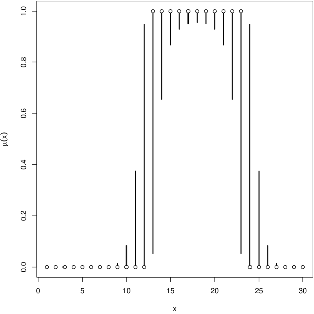
G.4 Linearity by computational geometry
Calculate linearity using R package rcdd like
in Section F.5 above.
\MakeFramed
## calling glm to:
## 1) get model matrix and
## 2) illustrate that it outputs a warning message when fit to this data
out <- glm(y ~ x + I(x^2), family = "binomial",
  data = quadratic, x = TRUE)
## Warning: glm.fit: algorithm did not converge
## Warning: glm.fit: fitted probabilities numerically 0 or 1 occurred
tanv <- modmat <- out$x
tanv[y == 1, ] <- (-tanv[y == 1, ])
vrep <- makeV(rays = tanv)
lout <- linearity(d2q(vrep), rep = "V")
lout
## integer(0)
So this agrees with our analysis in Section G.2 above.
G.5 Generic direction of recession
Calculate a GDOR using R package rcdd like
in Section F.6 above.
\MakeFramed
p <- ncol(tanv)
hrep <- cbind(0, 0, -tanv, -1)
hrep <- rbind(hrep, c(0, 1, rep(0, p), -1))
objv <- c(rep(0, p), 1)
pout <- lpcdd(d2q(hrep), d2q(objv), minimize = FALSE)
names(pout)
## [1] "solution.type"   "primal.solution" "dual.solution"
## [4] "optimal.value"
pout$solution.type
## [1] "Optimal"
gdor <- pout$primal.solution[1:p]
gdor
## [1] "-587/11" "72/11" "-2/11"
pout$optimal.value
## [1] "1"
This agrees with the GDOR found in the technical report (Geyer, 2008, Section 4.1) that is supplementary material for (Geyer, 2009). We clean R global environment.
\MakeFramed
rm(list = ls())
Appendix H Sports standings example of Geyer
This is the example in Section 2.4 of Geyer (2009). Its behavior is different from any of the preceding examples, because the LCM is not completely degenerate and also because the binomial sample size is two for all components of the response vector.
H.1 Data
Data
\MakeFramed
team.names <- c("ants", "beetles", "cows", "dogs",
    "egrets", "foxes", "gerbils", "hogs")
data <- matrix(c(NA, 2, 2, 2, 2, 2, 2, 2, 0, NA,
    1, 2, 2, 2, 2, 2, 0, 1, NA, 2, 1, 2, 2, 2, 0,
    0, 0, NA, 1, 1, 2, 2, 0, 0, 1, 1, NA, 1, 2, 2,
    0, 0, 0, 1, 1, NA, 2, 2, 0, 0, 0, 0, 0, 0, NA,
    1, 0, 0, 0, 0, 0, 0, 1, NA), byrow = TRUE, nrow = 8)
dimnames(data) <- list(team.names, team.names)
print(data)
##         ants beetles cows dogs egrets foxes gerbils hogs
## ants      NA       2    2    2      2     2       2    2
## beetles    0      NA    1    2      2     2       2    2
## cows       0       1   NA    2      1     2       2    2
## dogs       0       0    0   NA      1     1       2    2
## egrets     0       0    1    1     NA     1       2    2
## foxes      0       0    0    1      1    NA       2    2
## gerbils    0       0    0    0      0     0      NA    1
## hogs       0       0    0    0      0     0       1   NA
We model these data with Bradley-Terry model. We code this differently from the technical report (Geyer, 2008) accompanying Geyer (2009).
First we format the data the way R function glm likes
(in a data.frame).
\MakeFramed
wins <- data[upper.tri(data)]
team.plus <- row(data)[upper.tri(data)]
team.minus <- col(data)[upper.tri(data)]
modmat <- matrix(0, length(wins), nrow(data))
for (i in 1:ncol(modmat)) {
    modmat[team.plus == i, i] <- 1
    modmat[team.minus == i, i] <- (-1)
}
losses <- 2 - wins
resp <- cbind(wins, losses)

colnames(modmat) <- team.names
sportsdata <- cbind(modmat, wins, losses)
sportsdata <- as.data.frame(sportsdata)
These data are included in the glmdr package.
data(sports)
all.equal(sports, sportsdata)
## [1] TRUE
H.2 Fitting the Model
We first fit the model using the R function glmdr.
gout <- glmdr(cbind(wins, losses) ~ 0 + .,
  family = "binomial", data = sports)
summary(gout)
##
## MLE exists in Barndorff-Nielsen completion
## it is conditional on components of the response
## corresponding to object$linearity == FALSE being
## conditioned on their observed values
##
## GLM summary for limiting conditional model
##
##
## Call:
## stats::glm(formula = cbind(wins, losses) ~ 0 + ., family = "binomial",
##     data = sports, subset = c("3", "5", "6", "8", "9", "10",
##     "12", "13", "14", "15", "28"), x = TRUE, y = TRUE)
##
## Deviance Residuals:
##     Min       1Q   Median       3Q      Max
## -1.1692  -0.1970   0.3941   0.5038   0.6153
##
## Coefficients: (3 not defined because of singularities)
##           Estimate Std. Error z value Pr(>|z|)
## ants            NA         NA      NA       NA
## beetles  3.024e+00  1.487e+00   2.034   0.0419 *
## cows     2.310e+00  1.328e+00   1.740   0.0819 .
## dogs    -5.189e-17  1.080e+00   0.000   1.0000
## egrets   5.609e-01  1.078e+00   0.520   0.6029
## foxes           NA         NA      NA       NA
## gerbils  0.000e+00  1.414e+00   0.000   1.0000
## hogs            NA         NA      NA       NA
## ---
## Signif. codes:
## 0 ’***’ 0.001 ’**’ 0.01 ’*’ 0.05 ’.’ 0.1 ’ ’ 1
##
## (Dispersion parameter for binomial family taken to be 1)
##
##     Null deviance: 13.863  on 11  degrees of freedom
## Residual deviance:  3.391  on  6  degrees of freedom
## AIC: 21.709
##
## Number of Fisher Scoring iterations: 5
H.3 Linearity
As explained in Section 6.3 of the main text, the components of the response vector that are random in the LCM are those for which the null space projected to canonical parameter space of the saturated model have corresponding zeros. These components are those for which the linearity of the object returned by R function glmdr is true
\MakeFramed
gout$linearity
##     1     2     3     4     5     6     7     8     9    10
## FALSE FALSE  TRUE FALSE  TRUE  TRUE FALSE  TRUE  TRUE  TRUE
##    11    12    13    14    15    16    17    18    19    20
## FALSE  TRUE  TRUE  TRUE  TRUE FALSE FALSE FALSE FALSE FALSE
##    21    22    23    24    25    26    27    28
## FALSE FALSE FALSE FALSE FALSE FALSE FALSE  TRUE
H.4 Labels
We now want to make some confidence intervals, but first we make some
short labels for components of the response vector.
\MakeFramed
foo <- sports[ , ! (colnames(sports) %in% c("wins", "losses"))]
teams <- colnames(foo)
winner <- apply(foo == 1, 1, function(x) teams[x])
loser <- apply(foo == -1, 1, function(x) teams[x])
label <- paste(winner, "beat", loser)
head(label)
## [1] "ants beat beetles" "ants beat cows"
## [3] "beetles beat cows" "ants beat dogs"
## [5] "beetles beat dogs" "cows beat dogs"
H.5 Confidence Intervals
We now want to fit confidence intervals. These come in two kinds. First, there are confidence intervals for means of components of the response vector that are in the linearity. These are the usual sort of confidence intervals for GLM, based on asymptotics, and produced by the glm method of the R generic function predict. Second, there are confidence intervals for means of components of the response vector that are not in the linearity. These are non-asymptotic intervals, described in Section 4.3, and produced by R function inference in R package glmdr. These latter intervals are necessarily one-sided because the MLE mean value parameter estimates for these components of the response vector are on the boundary of the range of possible values.
H.5.1 Two-Sided Intervals
We get estimated means and standard errors as follows.
\MakeFramed
preds <- predict(gout$lcm, type = "response", se.fit = TRUE)
preds.tab <- cbind(preds$fit, preds$se.fit)
colnames(preds.tab) <- c("fit", "se")
rownames(preds.tab) <- label[gout$linearity]
round(preds.tab, 3)
##                       fit    se
## beetles beat cows   0.671 0.274
## beetles beat dogs   0.954 0.066
## cows beat dogs      0.910 0.109
## beetles beat egrets 0.921 0.103
## cows beat egrets    0.852 0.159
## dogs beat egrets    0.363 0.249
## beetles beat foxes  0.954 0.066
## cows beat foxes     0.910 0.109
## dogs beat foxes     0.500 0.270
## egrets beat foxes   0.637 0.249
## gerbils beat hogs   0.500 0.354
And turn this into 95% confidence intervals as follows.
\MakeFramed
ci.tab <- apply(preds.tab, 1, function(x) x[1] + c(-1,1) * qnorm(0.975) * x[2])
ci.tab <- t(ci.tab)
colnames(ci.tab) <- c("lwr", "upr")
round(ci.tab, 3)
##                        lwr   upr
## beetles beat cows    0.134 1.208
## beetles beat dogs    0.825 1.082
## cows beat dogs       0.696 1.123
## beetles beat egrets  0.720 1.123
## cows beat egrets     0.541 1.163
## dogs beat egrets    -0.126 0.852
## beetles beat foxes   0.825 1.082
## cows beat foxes      0.696 1.123
## dogs beat foxes     -0.029 1.029
## egrets beat foxes    0.148 1.126
## gerbils beat hogs   -0.193 1.193
As always, there is no reason why Wald confidence intervals cannot go outside the boundaries of the parameter space, as some of these intervals do. As noted in the discussion of (Geyer, 2009), the sample sizes here are by no means “large”. The last confidence interval (gerbils versus hogs) is based on exactly two games (these teams played two games and each won one, no other games are relevant to this inference). So for these data, the confidence intervals produced in this section are of questionable validity.
H.5.2 One-Sided Intervals
We get one-sided intervals as follows. These numbers agree with
Table 5 in (Geyer, 2009),
which was done by methods that are much more messy and made obsolete
by the methods presented here.
\MakeFramed
ci.tab.too <- inference(gout)
rownames(ci.tab.too) <- label[! gout$linearity]
round(ci.tab.too, 3)
##                      lower upper
## ants beat beetles    0.893     2
## ants beat cows       1.245     2
## ants beat dogs       1.886     2
## ants beat egrets     1.809     2
## ants beat foxes      1.886     2
## ants beat gerbils    1.993     2
## beetles beat gerbils 1.970     2
## cows beat gerbils    1.940     2
## dogs beat gerbils    1.526     2
## egrets beat gerbils  1.699     2
## foxes beat gerbils   1.526     2
## ants beat hogs       1.993     2
## beetles beat hogs    1.970     2
## cows beat hogs       1.940     2
## dogs beat hogs       1.526     2
## egrets beat hogs     1.699     2
## foxes beat hogs      1.526     2
With (each team plays each other team twice), quick and dirty confidence intervals go from zero to
(when ) or from
to one (again when ). None of the careful intervals calculated above are anywhere near as wide as the quick and dirty intervals.
H.6 Linearity by computational geometry
Calculate linearity using R package rcdd like
in Section F.5 above.
We follow Section 5 of J. (2009), except that seems to
have some errors, which we correct here.
\MakeFramed
tanv <- modmat
tanv[losses == 0, ] <- (- tanv[losses == 0, ])
vrep <- cbind(0, 0, tanv)
vrep[wins > 0 & losses > 0, 1] <- 1
lout <- linearity(d2q(vrep), rep = "V")
This result only includes the additional components found to be in the
linearity (in addition to the ones already known). So we have to add
the others to get the correct linearity.
\MakeFramed
linearity.too <- seq(along = wins) %in% lout
linearity.too[wins > 0 & losses > 0] <- TRUE
identical(as.vector(gout$linearity), linearity.too)
## [1] TRUE
So this agrees with our analysis in Section H.3 above.
H.7 Generic direction of recession
Calculate a GDOR using R package rcdd like
in Section F.6 above.
More specifically, we follow Section 6 of (Geyer, 2008),
so we necessarily agree with the GDOR given in Table 4 of (Geyer, 2009).
\MakeFramed
p <- ncol(tanv)
hrep <- cbind(0, 0, -tanv, 0)
hrep[! gout$linearity, ncol(hrep)] <- (-1)
hrep[gout$linearity, 1] <- 1
hrep <- rbind(hrep, c(0, 1, rep(0, p), -1))
objv <- c(rep(0, p), 1)
pout <- lpcdd(hrep, objv, minimize = FALSE)
gdor <- pout$primal.solution[1:p]
names(gdor) <- team.names
print(gdor)
##    ants beetles    cows    dogs  egrets   foxes gerbils
##       2       1       1       1       1       1       0
##    hogs
##       0
Clean R global environment.
rm(list = ls())
Appendix I Quasi-complete separation example of Agresti
I.1 Data
Agresti (2013, Section 6.5.1) introduces the notion of quasi-complete
separation
with the following example, which adds two data points to the data for
his other example (Section F above).
\MakeFramed
x <- seq(10, 90, 10)
x <- x[x != 50]
y <- as.numeric(x > 50)
x <- c(x, 50, 50)
y <- c(y, 0, 1)
These data are included in the glmdr package.
data(quasi)
all.equal(quasi, data.frame(x, y))
## [1] TRUE
I.2 Maximizing the OM likelihood
Again, we fit these data using R function glmdr.
gout <- glmdr(y ~ x, family = "binomial", data = quasi)
summary(gout)
##
## MLE exists in Barndorff-Nielsen completion
## it is conditional on components of the response
## corresponding to object$linearity == FALSE being
## conditioned on their observed values
##
## GLM summary for limiting conditional model
##
##
## Call:
## stats::glm(formula = y ~ x, family = "binomial", data = quasi,
##     subset = c("9", "10"), x = TRUE, y = TRUE)
##
## Deviance Residuals:
##      9      10
## -1.177   1.177
##
## Coefficients: (1 not defined because of singularities)
##              Estimate Std. Error z value Pr(>|z|)
## (Intercept) 4.710e-16  1.414e+00       0        1
## x                  NA         NA      NA       NA
##
## (Dispersion parameter for binomial family taken to be 1)
##
##     Null deviance: 2.7726  on 1  degrees of freedom
## Residual deviance: 2.7726  on 1  degrees of freedom
## AIC: 4.7726
##
## Number of Fisher Scoring iterations: 2
I.3 Linearity
We extract the linearity from the glmdr function call.
gout$linearity
##     1     2     3     4     5     6     7     8     9    10
## FALSE FALSE FALSE FALSE FALSE FALSE FALSE FALSE  TRUE  TRUE
I.4 One-sided confidence intervals for mean value parameters
We now provide one-sided confidence intervals for mean value parameters whose MLE is on the boundary.
inference(gout)
##       lower      upper
## 1 0.0000000 0.07082447
## 2 0.0000000 0.14043775
## 3 0.0000000 0.27199887
## 4 0.0000000 0.51720648
## 5 0.4827935 1.00000000
## 6 0.7280012 1.00000000
## 7 0.8595623 1.00000000
## 8 0.9291755 1.00000000
Note that for some components of the mean value parameter vector the lower or upper bound of our confidence interval is not close to the quick and dirty limit (Section F.3.2 above) like they were in the case of complete separation.
I.5 Two-sided confidence intervals for mean value parameters
As in the preceding example, confidence intervals for means of components
of the response vector in the linearity are given by R generic function
predict.
\MakeFramed
preds <- predict(gout$lcm, type = "response", se.fit = TRUE)
preds.tab <- cbind(preds$fit - qnorm(0.975) * preds$se.fit,
    preds$fit + qnorm(0.975) * preds$se.fit)
colnames(preds.tab) <- c("lower", "upper")
round(preds.tab, 3)
##     lower upper
## 9  -0.193 1.193
## 10 -0.193 1.193
As we saw with the sports data, these asymptotic confidence intervals are not good for toy data. Again we effectively have for these intervals, so they are exactly the same as the one for gerbils versus hogs in the sports data.
Clean R global environment.
\MakeFramed
rm(list = ls())
Appendix J Categorical data analysis example of Geyer
J.1 Data
This is the example in Section 2.3 of Geyer (2009). Its behavior
is very similar to the quasi-complete separation example
of Agresti in Section I above.
\MakeFramed
foo <- "https://conservancy.umn.edu/bitstream/handle/11299/197369/catrec.txt"
bar <- sub("^.*/", "", foo)
if (! file.exists(bar))
    download.file(foo, bar)
dat <- read.table(bar, header = TRUE)
dim(dat)
## [1] 128 8
names(dat)
## [1] "v1" "v2" "v3" "v4" "v5" "v6" "v7" "y"
These data are included in the glmdr package.
data(catrec)
all.equal(catrec, dat)
## [1] TRUE
J.2 Fitting the Model
Following Geyer (2009) we assume Poisson rather than multinomial
sampling. These two sampling schemes have the same MLE, even when the MLE
is in the Barndorff-Nielsen completion
[Agresti, 2013, Section 8.6.7; Geyer, 2009, Section 3.17]
but Poisson sampling is the easiest to fit.
We can use R function glm if the MLE exists in the conventional
sense, and R function glmdr otherwise.
\MakeFramed
gout <- glmdr(y ~ (v1 + v2 + v3 + v4 + v5 + v6 + v7)^3,
    family = "poisson", data = dat)
summary(gout)
##
## MLE exists in Barndorff-Nielsen completion
## it is conditional on components of the response
## corresponding to object$linearity == FALSE being
## conditioned on their observed values
##
## GLM summary for limiting conditional model
##
##
## Call:
## stats::glm(formula = y ~ (v1 + v2 + v3 + v4 + v5 + v6 + v7)^3,
##     family = "poisson", data = dat, subset = c("2", "3", "4",
##     "5", "6", "7", "8", "10", "11", "12", "13", "14", "15", "16",
##     "17", "18", "19", "21", "22", "23", "24", "25", "26", "27",
##     "29", "30", "31", "32", "34", "35", "36", "37", "38", "39",
##     "40", "42", "43", "44", "45", "46", "47", "48", "49", "50",
##     "51", "53", "54", "55", "56", "57", "58", "59", "61", "62",
##     "63", "64", "66", "67", "68", "69", "70", "71", "72", "74",
##     "75", "76", "77", "78", "79", "80", "81", "82", "83", "85",
##     "86", "87", "88", "89", "90", "91", "93", "94", "95", "96",
##     "98", "99", "100", "101", "102", "103", "104", "106", "107",
##     "108", "109", "110", "111", "112", "113", "114", "115", "117",
##     "118", "119", "120", "121", "122", "123", "125", "126", "127",
##     "128"), x = TRUE, y = TRUE)
##
## Deviance Residuals:
##      Min        1Q    Median        3Q       Max
## -1.63571  -0.30009  -0.02353   0.27258   1.42540
##
## Coefficients: (1 not defined because of singularities)
##              Estimate Std. Error z value Pr(>|z|)
## (Intercept)  2.150481   0.585423   3.673 0.000239 ***
## v1           0.069795   0.587067   0.119 0.905364
## v2          -0.524215   0.513583  -1.021 0.307396
## v3           0.052966   0.551965   0.096 0.923552
## v4          -0.709525   0.580147  -1.223 0.221326
## v5           0.243002   0.548686   0.443 0.657853
## v6          -1.163256   0.563668  -2.064 0.039044 *
## v7          -0.990704   0.597335  -1.659 0.097208 .
## v1:v2        0.384345   0.543024   0.708 0.479079
## v1:v3       -0.630375   0.570151  -1.106 0.268888
## v1:v4        0.008801   0.511458   0.017 0.986271
## v1:v5       -1.022805   0.570440  -1.793 0.072971 .
## v1:v6        0.540164   0.493879   1.094 0.274079
## v1:v7        0.097178   0.536628   0.181 0.856297
## v2:v3        0.602411   0.437371   1.377 0.168405
## v2:v4        0.748226   0.486811   1.537 0.124295
## v2:v5       -0.068926   0.428100  -0.161 0.872090
## v2:v6        0.297165   0.487409   0.610 0.542071
## v2:v7        0.274198   0.508369   0.539 0.589634
## v3:v4       -0.124465   0.541056  -0.230 0.818060
## v3:v5       -0.439354   0.468418  -0.938 0.348268
## v3:v6        0.024399   0.530220   0.046 0.963296
## v3:v7       -0.104400   0.556960  -0.187 0.851310
## v4:v5       -0.169421   0.521323  -0.325 0.745194
## v4:v6        0.756513   0.474213   1.595 0.110644
## v4:v7        0.780671   0.500911   1.559 0.119114
## v5:v6        1.245629   0.510770   2.439 0.014739 *
## v5:v7       -0.262620   0.523125  -0.502 0.615652
## v6:v7        0.697014   0.489957   1.423 0.154852
## v1:v2:v3    -0.349902   0.483330  -0.724 0.469102
## v1:v2:v4     0.101569   0.389778   0.261 0.794416
## v1:v2:v5     0.655208   0.493737   1.327 0.184496
## v1:v2:v6    -0.329286   0.390979  -0.842 0.399670
## v1:v2:v7    -0.520368   0.393042  -1.324 0.185520
## v1:v3:v4     0.353292   0.406623   0.869 0.384932
## v1:v3:v5     0.638711   0.484979   1.317 0.187843
## v1:v3:v6     0.352694   0.402715   0.876 0.381143
## v1:v3:v7    -0.001586   0.413554  -0.004 0.996941
## v1:v4:v5     0.664745   0.400212   1.661 0.096717 .
## v1:v4:v6    -0.463885   0.368214  -1.260 0.207732
## v1:v4:v7    -0.342583   0.372009  -0.921 0.357103
## v1:v5:v6     0.044968   0.399958   0.112 0.910481
## v1:v5:v7     0.447641   0.404364   1.107 0.268283
## v1:v6:v7     0.218868   0.371499   0.589 0.555763
## v2:v3:v4    -0.325914   0.404392  -0.806 0.420280
## v2:v3:v5           NA         NA      NA       NA
## v2:v3:v6    -0.247853   0.405621  -0.611 0.541168
## v2:v3:v7     0.028322   0.414520   0.068 0.945527
## v2:v4:v5     0.004655   0.394418   0.012 0.990583
## v2:v4:v6    -0.111152   0.373713  -0.297 0.766141
## v2:v4:v7    -0.148061   0.376692  -0.393 0.694279
## v2:v5:v6    -0.766051   0.394925  -1.940 0.052412 .
## v2:v5:v7     0.075213   0.399004   0.189 0.850482
## v2:v6:v7     0.460826   0.381109   1.209 0.226597
## v3:v4:v5    -0.063494   0.423318  -0.150 0.880771
## v3:v4:v6     0.357746   0.366298   0.977 0.328741
## v3:v4:v7    -0.106368   0.371567  -0.286 0.774672
## v3:v5:v6    -0.234816   0.422424  -0.556 0.578295
## v3:v5:v7     0.804923   0.423843   1.899 0.057550 .
## v3:v6:v7    -0.659090   0.371085  -1.776 0.075714 .
## v4:v5:v6    -0.427957   0.375755  -1.139 0.254734
## v4:v5:v7     0.125167   0.377356   0.332 0.740119
## v4:v6:v7     0.014192   0.370131   0.038 0.969413
## v5:v6:v7    -0.811516   0.377098  -2.152 0.031397 *
## ---
## Signif. codes:
## 0 ’***’ 0.001 ’**’ 0.01 ’*’ 0.05 ’.’ 0.1 ’ ’ 1
##
## (Dispersion parameter for poisson family taken to be 1)
##
##     Null deviance: 156.215  on 111  degrees of freedom
## Residual deviance:  31.291  on  49  degrees of freedom
## AIC: 526.46
##
## Number of Fisher Scoring iterations: 5
J.3 Linearity
We then find the linearity as in preceding sections.
\MakeFramed
linearity <- gout$linearity
catrec[!linearity, ]
##     v1 v2 v3 v4 v5 v6 v7 y
## 1    0  0  0  0  0  0  0 0
## 9    0  0  0  1  0  0  0 0
## 20   1  1  0  0  1  0  0 0
## 28   1  1  0  1  1  0  0 0
## 33   0  0  0  0  0  1  0 0
## 41   0  0  0  1  0  1  0 0
## 52   1  1  0  0  1  1  0 0
## 60   1  1  0  1  1  1  0 0
## 65   0  0  0  0  0  0  1 0
## 73   0  0  0  1  0  0  1 0
## 84   1  1  0  0  1  0  1 0
## 92   1  1  0  1  1  0  1 0
## 97   0  0  0  0  0  1  1 0
## 105  0  0  0  1  0  1  1 0
## 116  1  1  0  0  1  1  1 0
## 124  1  1  0  1  1  1  1 0
This agrees with (part of) Table 2 in (Geyer, 2009).
J.4 One-sided confidence intervals: Poisson sampling
We now provide one-sided confidence intervals for mean value parameters whose MLE is on the boundary as done before.
system.time(tab <- inference(gout))
##    user  system elapsed
##   0.564   0.012   0.578
upper <- tab$upper
cbind(catrec[!linearity, ], upper)
##     v1 v2 v3 v4 v5 v6 v7 y      upper
## 1    0  0  0  0  0  0  0 0 0.28630976
## 9    0  0  0  1  0  0  0 0 0.14082947
## 20   1  1  0  0  1  0  0 0 0.21996699
## 28   1  1  0  1  1  0  0 0 0.42095570
## 33   0  0  0  0  0  1  0 0 0.08946242
## 41   0  0  0  1  0  1  0 0 0.09376644
## 52   1  1  0  0  1  1  0 0 0.19302341
## 60   1  1  0  1  1  1  0 0 0.28869770
## 65   0  0  0  0  0  0  1 0 0.10631113
## 73   0  0  0  1  0  0  1 0 0.11415034
## 84   1  1  0  0  1  0  1 0 0.09128766
## 92   1  1  0  1  1  0  1 0 0.26461098
## 97   0  0  0  0  0  1  1 0 0.06669488
## 105  0  0  0  1  0  1  1 0 0.15477613
## 116  1  1  0  0  1  1  1 0 0.14096916
## 124  1  1  0  1  1  1  1 0 0.32392016
This agrees with Table 2 in (Geyer, 2009).
J.4.1 Theory
Here we modify Section F.3.1 above, changing what needs to be changed for Poisson regression rather than logistic regression.
As in Section F.3.1 above,
let denote the vector of submodel canonical parameters,
let denote the log likelihood,
and let denote an MLE in the LCM.
We will use
the vector gout$lcm$coefficients with NA values
replaced by zeros.
Let denote the index set of the components of the response vector
on which we condition the OM to get the LCM (the indices of components of
linearity that are FALSE), and let and
denote the corresponding components of the response vector considered
as a random vector and as an observed
value, respectively. Then endpoints for a confidence
interval for a scalar parameter are given
by (6), when it does give a one-sided interval.
Since the only boundary of the mean value parameter space of the Poisson distribution is zero, in this section, we will be doing confidence intervals for mean value parameters for cells of the contingency table where the MLE in the LCM is zero. And we know the min is zero, so we only have to calculate the max.
In (6) denotes probability with respect to the OM not the LCM. As always in categorical data analysis, we have different possible sampling models: Poisson, multinomial, and product multinomial. So we get different intervals depending on which sampling model we use. In this section we are assuming Poisson.
Let denote the model matrix. Let denote the saturated model canonical parameter (usually called “linear predictor” in GLM theory).
Let denote the mean value parameter (here operates componentwise like the R function of the same name does), then
We could take the confidence interval problem to be
| (48) |
where is taken to be the function of described above. And this can be done for any .
But the problem will be more computationally stable if we state it as
| (49) |
Since is a monotone transformation and log is a monotone transformation, the two problems are equivalent (a solution for one is also a solution for the other).
We maximize canonical rather than mean value parameters to avoid extreme inexactness of computer arithmetic in calculating mean value parameters near zero. We take logs in the constraint for the same reasons we take logs of likelihoods.
Because optimizers expect to optimize over for some , let be a matrix whose columns are a basis for (the R matrix nulls calculated above, for example). Then every can be written as for some , where is the column dimension of and the dimension of .
To an optimizer (we will use R function auglag in CRAN package alabama) problem (49) has the abstract form (47) and the optimization works better if derivatives of and are provided. Because R function auglag only does minimization, the objective function must be the negation of what we have in (49). That is
where are the components of .
J.4.2 Quick and dirty intervals
As a sanity check and as a quick and dirty conservative (perhaps very conservative) confidence interval, we note that since all the are nonnegative, the only way the constraint in (48) can be satisfied is if . For this upper bound is -. No upper bound for a one-sided 95% confidence interval for the mean value parameter for a cell for which the MLE in the LCM is zero can be larger than that.
J.5 One-sided confidence intervals: Multinomial sampling
J.5.1 Theory
We use the same notation as in Section J.4.1 above, except where modified here.
Since the only boundary of the mean value parameter space of the multinomial distribution is where one or more components of the state vector are zero, we will be doing confidence intervals for mean value parameters for cells of the contingency table where the MLE in the LCM is zero. And we know the min is zero, so we only have to calculate the max. (If the MLE in the LCM for mean value parameter vector had all but one component equal to zero, so the other was equal to one, then we could make one-sided intervals for all components. But that is not a situation we see in any of our examples, and we will leave that as an exercise for the reader.)
For multinomial sampling, contingency table cell probabilities are defined by
| (50) |
where is the index set for the whole table.
Now
where
is the multinomial sample size, where is the index set of the cells that have mean value zero for the MLE in the LCM.
So we could take the confidence interval problem to be
| (51) |
where is taken to be the function of described above. And this can be done for any .
Unlike preceding theory for this problem, we cannot take to be the objective function because is not a function of only (much less a monotone function of it). Consequently, to obtain computational stability, we will take logs of both equations obtaining
| (52) |
The parameterization (50) introduces a direction of constancy (DOC) (Geyer, 2009, Theorem 1 and the following discussion) that is the same as the DOC we had in the Bradley-Terry model (Section H above), the vector all of whose components are the same.
So perhaps we should redo our null space of the Fisher information matrix calculation using the multinomial distribution. But this is not necessary. Movement along the DOC does not change any of the so does not change any of the equations in either of our optimization problems. We do not need to add it to the null space we obtained from the Poisson analysis. (Section 3.17 in (Geyer, 2009) shows that every DOR for the Poisson model is also a DOR for the multinomial model.)
Thus our problem has the abstract form (47) with
| (53) | ||||
| (54) |
where are the components of , and
| (55) | ||||
| (56) | ||||
where
( is the vector of probabilities in the OM, is the vector of probabilities in the LCM).
J.5.2 Quick and dirty intervals
If for some , then
Introducing we get
for large . Thus this agrees with our analysis in Section J.4.2 when is large.
We get the exact inequality
or
or
when , which is what it is in this example, and . And this too agrees approximately with our analysis in Section J.4.2 above.
J.5.3 Careful coding
We can modify (53) above as
where is any real number. We avoid overflow and catastrophic cancellation if we choose
in which case we have
in which overflow cannot occur and we avoid catastrophic cancellation in for small .
We can modify (55) above as
where and are any real numbers. We avoid overflow and catastrophic cancellation if we choose as above and
in which case we have
in which overflow cannot occur and we avoid catastrophic cancellation in for small .
J.6 Linearity by computational geometry
Calculate linearity using R package rcdd like in Section F.5 above. We follow Section 4.2 of (Geyer, 2008).
tanv <- gout$modmat
vrep <- cbind(0, 0, tanv)
vrep[dat$y > 0, 1] <- 1
system.time(lout <- linearity(d2q(vrep), rep = "V"))
##    user  system elapsed
##   4.334   0.003   4.337
linearity.too <- dat$y > 0
linearity.too[lout] <- TRUE
identical(as.vector(linearity), linearity.too)
## [1] TRUE
So this agrees with our analysis in Section J.3 above, except that the repeated linear programming implementation is slower than the implementation developed here.
J.7 Generic direction of recession
We calculate a GDOR using R package rcdd as in Section F.6 above. More specifically, we follow Section 4.2 of (Geyer, 2008), so we necessarily agree with the GDOR given in Table 1 of (Geyer, 2009).
modmat <- gout$modmat
hrep <- cbind(0, 0, -tanv, 0)
hrep[! linearity, ncol(hrep)] <- (-1)
hrep[linearity, 1] <- 1
hrep <- rbind(hrep, c(0, 1, rep(0, ncol(gout$modmat)), -1))
objv <- c(rep(0, ncol(gout$modmat)), 1)
pout <- lpcdd(d2q(hrep), d2q(objv), minimize = FALSE)
gdor <- pout$primal.solution[-length(pout$primal.solution)]

foo <- gdor
names(foo) <- colnames(modmat)
cbind(foo[foo != "0"])
##             [,1]
## (Intercept) "-1"
## v1          "1"
## v2          "1"
## v3          "1"
## v5          "1"
## v1:v2       "-1"
## v1:v3       "-1"
## v1:v5       "-1"
## v2:v3       "-1"
## v2:v5       "-1"
## v3:v5       "-1"
## v1:v2:v3    "1"
## v1:v3:v5    "1"
## v2:v3:v5    "1"
This agrees with Table 1 in (Geyer, 2009). Clean R global environment.
rm(list = ls())
Appendix K A big data example
K.1 Data
Load the data.
\MakeFramed
foo <- "https://conservancy.umn.edu/bitstream/handle/11299/197369/bigcategorical.txt"
bar <- sub("^.*/", "", foo)
if (! file.exists(bar))
    download.file(foo, bar)
dat <- read.table(bar, header = TRUE, stringsAsFactors = TRUE)
dim(dat)
## [1] 1024 6
names(dat)
## [1] "x1" "x2" "x3" "x4" "x5" "y"
The response vector is y, the predictors x1 through x5 are all categorical. The components of y are all counts, so this is a categorical data analysis. This contingency table has 1024 cells and the multinomial sample size (sum of cell counts) is 1055. These data are included in the glmdr package.
data(bigcategorical)
all.equal(dat, bigcategorical)
## [1] TRUE
K.2 Hypothesis Tests
As in Section J above, we assume a Poisson sampling model rather than a multinomial sampling model for the reasons stated in that section. Actually, as is well known (Agresti, 2013, Section 8.6.7), the MLE for the mean value parameter vector and the asymptotic chi-square distribution of test statistics is the same for Poisson, multinomial, and product multinomial sampling. So nothing in this section depends on the sampling model.
out1 <- glm(y ~ 0 + .,
    family = poisson, data = dat, x = TRUE,
    control = list(maxit = 1e3, epsilon = 1e-12))
out2 <- glm(y ~ 0 + (.)^2,
    family = poisson, data = dat, x = TRUE,
    control = list(maxit = 1e3, epsilon = 1e-12))
out3 <- glm(y ~ 0 + (.)^3,
    family = poisson, data = dat, x = TRUE,
    control = list(maxit = 1e3, epsilon = 1e-12))
out4 <- glm(y ~ 0 + (.)^4,
    family = poisson, data = dat, x = TRUE,
    control = list(maxit = 1e3, epsilon = 1e-12))
## Warning: glm.fit: fitted rates numerically 0 occurred
anova(out1, out2, out3, out4, test = "Chisq")
## Analysis of Deviance Table
##
## Model 1: y ~ 0 + (x1 + x2 + x3 + x4 + x5)
## Model 2: y ~ 0 + (x1 + x2 + x3 + x4 + x5)^2
## Model 3: y ~ 0 + (x1 + x2 + x3 + x4 + x5)^3
## Model 4: y ~ 0 + (x1 + x2 + x3 + x4 + x5)^4
##   Resid. Df Resid. Dev  Df Deviance  Pr(>Chi)
## 1      1008    1182.17
## 2       918    1076.55  90   105.62    0.1247
## 3       648     811.73 270   264.83    0.5774
## 4       243     277.37 405   534.36 1.605e-05 ***
## ---
## Signif. codes:
## 0 ’***’ 0.001 ’**’ 0.01 ’*’ 0.05 ’.’ 0.1 ’ ’ 1
Despite the warning from R function glm, all of these hypothesis tests are valid because in none of them is gout4 the null hypothesis. Tests done as in Table 2 in the main text.
anova(out1, out4, test = "Chisq")
## Analysis of Deviance Table
##
## Model 1: y ~ 0 + (x1 + x2 + x3 + x4 + x5)
## Model 2: y ~ 0 + (x1 + x2 + x3 + x4 + x5)^4
##   Resid. Df Resid. Dev  Df Deviance  Pr(>Chi)
## 1      1008    1182.17
## 2       243     277.37 765    904.8 0.0003447 ***
## ---
## Signif. codes:
## 0 ’***’ 0.001 ’**’ 0.01 ’*’ 0.05 ’.’ 0.1 ’ ’ 1
anova(out2, out4, test = "Chisq")
## Analysis of Deviance Table
##
## Model 1: y ~ 0 + (x1 + x2 + x3 + x4 + x5)^2
## Model 2: y ~ 0 + (x1 + x2 + x3 + x4 + x5)^4
##   Resid. Df Resid. Dev  Df Deviance  Pr(>Chi)
## 1       918    1076.55
## 2       243     277.37 675   799.18 0.0006633 ***
## ---
## Signif. codes:
## 0 ’***’ 0.001 ’**’ 0.01 ’*’ 0.05 ’.’ 0.1 ’ ’ 1
anova(out3, out4, test = "Chisq")
## Analysis of Deviance Table
##
## Model 1: y ~ 0 + (x1 + x2 + x3 + x4 + x5)^3
## Model 2: y ~ 0 + (x1 + x2 + x3 + x4 + x5)^4
##   Resid. Df Resid. Dev  Df Deviance  Pr(>Chi)
## 1       648     811.73
## 2       243     277.37 405   534.36 1.605e-05 ***
## ---
## Signif. codes:
## 0 ’***’ 0.001 ’**’ 0.01 ’*’ 0.05 ’.’ 0.1 ’ ’ 1
These agree with Table 2 in the main text.
K.3 Maximizing the likelihood
We fit these data using R function glmdr.
gout <- glmdr(y ~ 0 + (.)^4, family = "poisson",
  data = bigcategorical)
K.4 Linearity
We then find the linearity as in preceding sections.
linearity <- gout$linearity
sum(linearity)
## [1] 942
sum(! linearity)
## [1] 82
K.5 One-sided confidence intervals: Poisson sampling
We now provide one-sided confidence intervals for mean value parameters whose MLE is on the boundary as done before. This is the full table referenced in the main text.
system.time(mus.CI <- inference(gout))
##    user  system elapsed
##  57.416 161.807  60.102
upper <- round(mus.CI[, ncol(mus.CI)], 4)
tab <- cbind(dat[!linearity, ], upper)
tab
##      x1 x2 x3 x4 x5 y  upper
## 17    a  a  b  a  a 0 0.1695
## 21    a  b  b  a  a 0 0.1354
## 25    a  c  b  a  a 0 0.2292
## 29    a  d  b  a  a 0 2.4616
## 48    d  d  c  a  a 0 0.0002
## 57    a  c  d  a  a 0 0.0133
## 58    b  c  d  a  a 0 0.5647
## 59    c  c  d  a  a 0 0.2790
## 60    d  c  d  a  a 0 2.1519
## 105   a  c  c  b  a 0 0.1060
## 106   b  c  c  b  a 0 0.6088
## 107   c  c  c  b  a 0 2.2809
## 108   d  c  c  b  a 0 1.4718
## 112   d  d  c  b  a 0 2.9921
## 121   a  c  d  b  a 0 0.0167
## 176   d  d  c  c  a 0 0.0008
## 183   c  b  d  c  a 0 0.0103
## 185   a  c  d  c  a 0 2.9448
## 222   b  d  b  d  a 0 0.0607
## 240   d  d  c  d  a 0 0.0027
## 249   a  c  d  d  a 0 0.0509
## 285   a  d  b  a  b 0 1.8519
## 286   b  d  b  a  b 0 0.0995
## 287   c  d  b  a  b 0 0.0027
## 288   d  d  b  a  b 0 1.1411
## 297   a  c  c  a  b 0 2.8903
## 301   a  d  c  a  b 0 2.2144
## 350   b  d  b  b  b 0 2.9408
## 361   a  c  c  b  b 0 0.0850
## 364   d  c  c  b  b 0 0.0154
## 365   a  d  c  b  b 0 0.6450
## 377   a  c  d  b  b 0 2.8350
## 397   a  d  a  c  b 0 2.9956
## 413   a  d  b  c  b 0 0.0001
## 414   b  d  b  c  b 0 0.0549
## 417   a  a  c  c  b 0 0.5509
## 421   a  b  c  c  b 0 2.4449
## 425   a  c  c  c  b 0 0.0860
## 429   a  d  c  c  b 0 0.0004
## 439   c  b  d  c  b 0 2.0680
## 445   a  d  d  c  b 0 0.0000
## 478   b  d  b  d  b 0 0.2229
## 489   a  c  c  d  b 0 0.0204
## 493   a  d  c  d  b 0 0.1364
## 505   a  c  d  d  b 0 1.2175
## 506   b  c  d  d  b 0 0.2057
## 507   c  c  d  d  b 0 1.5164
## 508   d  c  d  d  b 0 0.0560
## 517   a  b  a  a  c 0 1.1298
## 518   b  b  a  a  c 0 1.0333
## 519   c  b  a  a  c 0 0.1836
## 520   d  b  a  a  c 0 0.6489
## 525   a  d  a  a  c 0 0.0570
## 541   a  d  b  a  c 0 2.8136
## 557   a  d  c  a  c 0 0.0098
## 573   a  d  d  a  c 0 0.1153
## 588   d  c  a  b  c 0 2.4637
## 604   d  c  b  b  c 0 0.2193
## 620   d  c  c  b  c 0 0.0064
## 633   a  c  d  b  c 0 0.1588
## 636   d  c  d  b  c 0 0.3127
## 695   c  b  d  c  c 0 0.4586
## 734   b  d  b  d  c 0 0.0004
## 793   a  c  b  a  d 0 2.6538
## 834   b  a  a  b  d 0 0.0049
## 850   b  a  b  b  d 0 0.0008
## 857   a  c  b  b  d 0 0.0392
## 866   b  a  c  b  d 0 0.0019
## 876   d  c  c  b  d 0 2.9803
## 882   b  a  d  b  d 0 2.9881
## 889   a  c  d  b  d 0 0.0018
## 921   a  c  b  c  d 0 0.0484
## 951   c  b  d  c  d 0 0.4589
## 965   a  b  a  d  d 0 0.2902
## 981   a  b  b  d  d 0 1.9221
## 985   a  c  b  d  d 0 0.2544
## 990   b  d  b  d  d 0 2.9346
## 997   a  b  c  d  d 0 0.7834
## 1009  a  a  d  d  d 0 2.9673
## 1013  a  b  d  d  d 0 0.0169
## 1017  a  c  d  d  d 0 0.0211
## 1021  a  d  d  d  d 0 0.0073
Table 3 in the main text is provided below
head(tab)
##    x1 x2 x3 x4 x5 y  upper
## 17  a  a  b  a  a 0 0.1695
## 21  a  b  b  a  a 0 0.1354
## 25  a  c  b  a  a 0 0.2292
## 29  a  d  b  a  a 0 2.4616
## 48  d  d  c  a  a 0 0.0002
## 57  a  c  d  a  a 0 0.0133
This also agrees with the first version of this document, which took several hours to do this job (and we are taking only a few seconds).
K.6 Linearity by computational geometry
Calculate linearity using R package rcdd like
in Section J.6 above.
Except that we are going to cache the result and the time it takes
to compute it. Rather than using the cache feature of R package
knitr, which should not be committed under version control,
we cache it ourselves.
\MakeFramed
tanv <- modmat <- out4$x
vrep <- cbind(0, 0, tanv)
vrep[dat$y > 0, 1] <- 1
suppressWarnings(foo <- try(load("foo-linearity.rda"), silent = TRUE))
if (inherits(foo, "try-error")) {
    time.linearity.big.data <- system.time(
        lout <- linearity(d2q(vrep), rep = "V")
    )
    hostname.linearity.big.data <- NULL
    cpuinfo.linearity.big.data <- NULL
    if (Sys.info()["sysname"] == "Linux") {
        foo <- scan("/proc/cpuinfo", what = character(0), sep = "\n")
        bar <- grep("^model name", foo, value = TRUE)
        bar <- unique(bar)
        baz <- sub("^model name\\t: ", "", bar)
        qux <- system("nslookup ‘hostname‘", intern = TRUE)
        quux <- grep("^Name:", qux, value = TRUE)
        quuux <- sub("^Name:\\t", "", quux)
        quacks <- unique(quuux)
        hostname.linearity.big.data <- quacks[1]
        cpuinfo.linearity.big.data <- baz
    }
    save(lout, time.linearity.big.data,
        hostname.linearity.big.data, cpuinfo.linearity.big.data,
        file = "foo-linearity.rda")
}
linearity.too <- dat$y > 0
linearity.too[lout] <- TRUE
identical(as.vector(linearity), linearity.too)
## [1] TRUE
References
- Agresti [2013] A. Agresti. Categorical Data Analysis. John Wiley & Sons, Hoboken, NJ, third edition, 2013.
- Aickin [1979] M. Aickin. Existence of mles for discrete linear exponential models. Annals of the Institute of Statistical Mathematics, 31(1):103–113, 1979.
- Albert and Anderson [1984] A. Albert and J. A. Anderson. On the existence of maximum likelihood estimates in logistic regression models. Biometrika, 71:1–10, 1984.
- Barndorff-Nielsen [1978] O. Barndorff-Nielsen. Information and Exponential Families In Statistical Theory. John Wiley & Sons, Chichester, 1978.
- Billingsley [1999] P. Billingsley. Convergence of Probability Measures. John Wiley & Sons, New York, second edition, 1999. doi: 10.1002/9780470316962.
- Billingsley [2012] P. Billingsley. Probability and Measure. John Wiley & Sons, Hoboken, NJ, anniversary edition, 2012.
- Brown [1986] L. D. Brown. Fundamentals of Statistical Exponential Families with Applications in Statistical Decision Theory. Institute of Mathematical Statistics, Hayward, CA, 1986.
- Candes and Sur [2019] E. Candes and P. Sur. The phase transition for the existence of the maximum likelihood estimate in high-dimensional logistic regression. Annals of Statistics, 2019. To appear.
- Csiszár and Matúš [2001] I. Csiszár and F. Matúš. Convex cores of measures on r d. Studia Scientiarum Mathematicarum Hungarica, 38(1-4):177–190, 2001.
- Csiszár and Matúš [2003] I. Csiszár and F. Matúš. Information projections revisited. IEEE Transactions on Information Theory, 49(6):1474–1490, 2003.
- Csiszár and Matúš [2005] I. Csiszár and F. Matúš. Closures of exponential families. Ann. Probab., 33:582–600, 2005. doi: 10.1214/009117904000000766.
- Csiszár and Matúš [2008] I. Csiszár and F. Matúš. Generalized maximum likelihood estimates for exponential families. Probab. Theory Relat. Fields, 141:213–246, 2008. doi: 10.1007/s00440-007-0084-z.
- [13] D. J. Eck and C. J. Geyer. Two data sets that are examples for an article titled “computationally efficient likelihood inference in exponential families when the maximum likelihood estimator does not exist”. http://hdl.handle.net/11299/197369.
- Eck et al. [2015] Daniel J Eck, Ruth G Shaw, Charles J Geyer, and Joel G Kingsolver. An integrated analysis of phenotypic selection on insect body size and development time. Evolution, 69(9):2525–2532, 2015.
- Eriksson et al. [2006] N. Eriksson, S. E. Fienberg, A. Rinaldo, and S. Sullivant. Polyhedral conditions for the nonexistence of the mle for hierarchical log-linear models. Journal of Symbolic Computation, 41(2):222–233, 2006.
- Fienberg and Rinaldo [2012] S. E. Fienberg and A. Rinaldo. Maximum likelihood estimation in log-linear models. Annals of Statistics, 40(2):996–1023, 2012.
- Geyer [1990] C. J. Geyer. Likelihood and Exponential Families. PhD thesis, University of Washington, 1990. http://hdl.handle.net/11299/56330.
- Geyer [1991] C. J. Geyer. Markov chain Monte Carlo maximum likelihood. In Computing Science and Statistics: Proc. 23rd Symp. Interface, pages 156–163, 1991. http://purl.umn.edu/58440.
- Geyer [1999] C. J. Geyer. Likelihood inference for spatial point processes. In Stochastic Geometry (Toulouse, 1996), pages 79–140. Chapman & Hall/CRC, Boca Raton, FL, 1999.
- Geyer [2008] C. J. Geyer. Supporting theory and data analysis for “likelihood inference in exponential families and directions of recession”. Technical Report 672, School of Statistics, University of Minnesota, 2008. http:www.stat.umn.edu/geyer/gdor/phaseTR.pdf.
- Geyer [2009] C. J. Geyer. Likelihood inference in exponential families and directions of recession. Electron. J. Stat., 3:259–289, 2009. doi: 10.1214/08-EJS349.
- Geyer [2016] C. J. Geyer. Two examples of agresti, 2016. http://www.stat.umn.edu/geyer/8931expfam/infinity.pdf, knitr source http://www.stat.umn.edu/geyer/8931expfam/infinity.Rnw.
- Geyer and Eck [2016] C. J. Geyer and D. J. Eck. R package glmdr: Exponential Family Generalized Linear Models Done Right, version 0.1, 2016. https://github.com/cjgeyer/glmdr/tree/master/package.
- Geyer and Møller [1994] C. J. Geyer and J. Møller. Simulation procedures and likelihood inference for spatial point processes. Scand. J. Statist., 21(4):359–373, 1994.
- Geyer and Thompson [1992] C. J. Geyer and E. A. Thompson. Constrained Monte Carlo maximum likelihood for dependent data (with discussion). J. Roy. Statist. Soc. Ser. B, 54(3):657–699, 1992.
- Geyer et al. [2007] C. J. Geyer, S. Wagenius, and R. G. Shaw. Aster models for life history analysis. Biometrika, 94(2):415–426, 2007.
- Geyer et al. [2017] C. J. Geyer, G. D. Meeden, and K. Fukuda. R package rcdd: Computational Geometry, version 1.2, 2017. https://CRAN.R-project.org/package=rcdd.
- Haberman [1974] S. J. Haberman. The Analysis of Frequency Data. Chicago Press, 1974.
- Halmos [1974] P. R. Halmos. Finite-Dimensional Vector Spaces. Springer-Verlag, New York, second edition, 1974. Reprint of 1958 edition published by Van Nostrand.
- Handcock et al. [2018] M. S. Handcock, D. R. Hunter, C. T. Butts, S. M. Goodreau, P. N. Krivitsky, and M. Morris. R package ergm: Fit, Simulate and Diagnose Exponential-Family Models for Networks, version 3.9.4, 2018. https://CRAN.R-project.org/package=ergm.
- Hunter et al. [2008] D. R. Hunter, M. S. Handcock, C. T. Butts, S. M. Goodreau, and M. Morris. ergm: A package to fit, simulate and diagnose exponential-family models for networks. Journal of Statistical Software, 24(3):1–29, 2008.
- J. [2009] Geyer. C. J. More supporting data analysis for “likelihood inference in exponential families and directions of recession”. Technical Report 673, School of Statistics, University of Minnesota, 2009. http:www.stat.umn.edu/geyer/gdor/phase2TR.pdf.
- Matúš [2015] F. Matúš. On limiting towards the boundaries of exponential families. Kybernetika, 51(5):725–738, 2015.
- Rinaldo et al. [2009] A. Rinaldo, S. E. Fienberg, and Y. Zhou. On the geometry of discrete exponential families with application to exponential random graph models. Electron. J. Stat., 3:446–484, 2009.
- Rockafellar [1970] R. T. Rockafellar. Convex Analysis. Princeton University Press, Princeton, NJ, 1970.
- Rockafellar and Wets [1998] R. T. Rockafellar and R. J.-B. Wets. Variational Analysis. Springer-Verlag, Berlin, 1998. doi: 10.1007/978-3-642-02431-3. Corrected printings contain extensive changes. We used the third corrected printing, 2010.
- Rudin [1991] W. Rudin. Functional Analysis. McGraw-Hill, New York, second edition, 1991.
- Santner and Duffy [1986] T. J. Santner and D. E. Duffy. A note on a. albert and ja anderson’s conditions for the existence of maximum likelihood estimates in logistic regression models. Biometrika, 73(3):755–758, 1986.
- Schweinberger [2011] M. Schweinberger. Instability, sensitivity, and degeneracy of discrete exponential families. J. Amer. Statist. Assoc., 106(496):1361–1370, 2011.
- Silvapulle and Burridge [1986] M. J. Silvapulle and J. Burridge. Existence of maximum likelihood estimates in regression models for grouped and ungrouped data. Journal of the Royal Statistical Society: Series B (Methodological), 48(1):100–106, 1986.
- Steen and Seebach [1978] L. A. Steen and J. A. Seebach, Jr. Counterexamples in Topology. Springer-Verlag, New York, second edition, 1978.
- Verbeek [1992] A. Verbeek. The compactification of generalized linear models. Statistica neerlandica, 46(2-3):107–142, 1992.
- Wang et al. [2019] N. Wang, J. Rauh, and H. Massam. Approximating faces of marginal polytopes in discrete hierarchical models. The Annals of Statistics, 47(3):1203–1233, 2019.
- Weyl [1912] H. Weyl. Das asymptotische Verteilungsgesetz der Eigenwerte linearer partieller Differentialgleichungen (mit einer Anwendung auf die Theorie der Hohlraumstrahlung). Mathematische Annalen, 71:441–479, 1912.