Convexity of Solvability Set of
Power Distribution Networks

Abstract

The solvability set of a power network – the set of all power injection vectors for which the corresponding Power Flow equations admit a solution – is central to power systems stability and security, as well as to the tightness of Optimal Power Flow relaxations. Whenever the solvability set is convex, this allows for substantial simplifications of various optimization and risk assessment algorithms. In this paper we focus on the solvability set of power distribution networks and prove convexity of the full solvability set (real and reactive powers) for tree homogeneous networks with the same $r/x$ ratio for all elements. We also show this result can not be improved: once the network is not homogeneous, the convexity is immediately lost. It is nevertheless the case that if the network is almost homogeneous, a substantial practically-important part of the solvability set is still convex. Finally, we prove convexity of real solvability set (only real powers) for any tree network as well as for purely resistive networks with arbitrary topology.

I Introduction

The solvability set of power networks, the set of all physically possible power injections, is the central object for power system voltage stability and security analysis. Whenever the operational point approaches the boundary of solvability, the power system may become unstable causing a blackout. In practice, physical constraints which follow directly from the Power Flow equations are often amended by various additional constraints, e.g. on maximal nodal injection or limitations on line transmission. The set of all powers satisfying both physical and the additional constraints is usually denoted as feasibility set. In this paper we primarily focus on the solvability set $F$, which we will define as the set of all power injections for which the corresponding Power Flow equations admit a solution.

The problem of the geometry of the power flow feasibility set has a long history with first discussions appearing as early as 1975 [1, 2]. The non-convexity of the general solvability sets have been explicitly demonstrated and discussed for example in [3, 4, 5]. Remarkably, optimization algorithms for OPF relying on convex relaxation often yield an exact result [6, 7]. This observation lead to a host of activities focusing on understanding applicability of convex optimization methods toward OPF. In particular it was established that different formulations of convex optimization algorithms for OPF with constraints are exact for certain types of networks, e.g. acyclic networks satisfying a set of realistic constraints [6, 7, 8, 9, 10, 11, 12, 13, 14]. In a related development certain geometrical properties of the feasibility sets for such networks were scrutinized in [15, 16, 17, 18]. These latter works provide a geometric explanation for the exactness of convex relaxation by showing that although the feasibility set is not convex, the Pareto front in such cases coincides with the Pareto front of the convex hull of the feasibility set. Accordingly, when the utility function is non-decreasing, the optimal point would belong to the Pareto front and hence would be the same for the original problem and the convex relaxed one.

In this paper we focus on establishing convexity of solvability set for several types of distribution networks. Whenever convexity is present this clearly simplifies associated OPF problems, allowing for an efficient solution for any convex utility function. This makes our work closely related to the previous studies on the subject. At the same time there is a substantial methodological difference between establishing convexity of the full feasibility set in our case and e.g. establishing exactness of convex relaxation discussed in [15, 16, 13, 14]. Speaking geometrically, latter works considered non-convex feasibility set and focused on a particular area of the boundary, the so-called Pareto front. This approach provides additional flexibility to incorporate various constraints, but it is not informative about the internal points of $F$ and can only explore the geometry of $F$ locally. Our approach surveys the whole boundary of the solvability set to detect potential boundary non-convexity. Crucially, it also involves a topological argument of [19, 20] which connects geometry of the boundary and convexity of the interior by ensuring that $F$ has no “holes” inside. Thus our approach is complementary to the convex optimization-based techniques and can establish global geometric properties of $F$, beyond the scope of the traditional convex analysis.

This paper is organized as follows. In the next section we introduce the notations and formulate the sufficient condition for convexity of [20]. We also explain its geometric interpretation. In section III we prove convexity of the full solvability set for homogeneous distribution networks with the tree topology. In section IV we discuss convexity of the real solvability set and prove its convexity for several different types of networks: arbitrary distribution networks with the tree topology and purely resistive networks with arbitrary topology. We conclude in section V.

II Notations and methodology

II-A Model and Notations

Throughout this paper we consider an AC model of power system consisting of $n$ PQ-buses $i=1,\dots,n$ and a slack bus $i=0$. The network is parametrized by a symmetric complex-valued admittance matrix $Y_{ik}$, $i,k=0,\dots,n$,

$$Y_{ik} = \left\{\begin{array}[]{c r}\sum_{l\sim i}y_{il}&{\rm\ if\ }i=k\\ -y_{ik}&{\rm\ if\ }i\sim k\\ 0&{\rm\ if\ }i\not\sim k\\ \end{array}\right.$$ (4)

By $i\sim k$ we denote that nodes $i$ and $k$ are connected. We further assume that in that case $y_{ik}\neq 0$. The power injection at node $i$ is given by (for $i=1,\dots,n$),

$$S_{i}=P_{i}+jQ_{i}=V_{i}\sum_{k\sim i}y^{*}_{ik}(V_{i}-V_{k})^{*}\ .$$ (5)

In our notations negative $P_{i}$ corresponds to power consumption and positive $P_{i}$ to power injection at node $i$. It is convenient to combine real and reactive powers into a vector $p=(P_{1},\dots,Q_{1},\dots)^{T}\in{\mathbb{R}}^{2n}$. The complex voltages $V_{i}$ for $i=1,\dots,n$ can be combined into a complex vector ${\bf V}=(V_{1},\dots)^{T}\in{\mathbb{C}}^{n}$ while slack voltage is taken to be $V_{0}\equiv 1$. The full solvability set $F\subset{\mathbb{R}}^{2n}$ is a set of all points $p\in{\mathbb{R}}^{2n}$ such that the system of Power Flow equations (5) is feasible (have a solution). Similarly we introduce the solvability set of real powers, or real solvability set, as the combination of all points $(P_{1},\dots,P_{n})^{T}\in{\mathbb{R}}^{n}$ such that the system of equations (5) is feasible at least for some $Q_{i}$.

One of the central objects in our approach is a linear combination of real and reactive powers

$$c\cdot p=\sum_{i=1}^{n}c_{i}P_{i}+\sum_{i=1}^{n}{c}_{n+i}Q_{i} = \sum_{i=1}^{n}\Re({\mathcal{C}}^{*}_{i}S_{i})\ ,$$ (6)

$$\mathcal{C}_{i} = {c}_{i}+j{c}_{n+i}\ .$$ (7)

Here we introduced $n$ complex variables ${\mathcal{C}}_{i}$ which encode a vector $c\in{\mathbb{R}}^{2n}$. For each $c\neq 0$, minimization problem

$$\arg\min_{p\in F}c\cdot p\ ,$$ (8)

gives the intersection points of the solvability set $F\subset{\mathbb{R}}^{2n}$ and the supporting hyperplane orthogonal to $c$. The same linear combination can be rewritten in matrix notations as

$$c\cdot p = {\bf V}^{\dagger}H_{c}{\bf V}-{\bf V}^{\dagger}J_{c}-J_{c}^{\dagger}{\bf V}\ ,$$ (9)

$$(H_{c})_{ik} = \left\{\begin{array}[]{l r}\Re({\mathcal{C}}_{i}\sum_{l\sim i}y_{il})&{\rm\ if\ }i=k\\ -(\mathcal{C}_{i}y_{ik}+\mathcal{C}_{k}^{*}y_{ik}^{*})/2&{\rm\ if\ }i\sim k\\ 0&{\rm\ if\ }i\not\sim k\\ \end{array}\right.$$ (13)

$$(J_{c})_{i} = \left\{\begin{array}[]{l r}\mathcal{C}_{i}y_{i0}/2&\qquad\qquad\ \ \quad{\rm if\ }i\sim 0\\ 0&{\rm if\ }i\not\sim 0\end{array}\right.\$$ (16)

II-B Sufficient Condition for Convexity

Real and reactive powers are the quadratic functions of voltages, $p=p(V)$. Hence the solvability set is an image of a particular quadratic map defined by (5). To establish convexity of solvability set we will rely on the result (Proposition 2’) of [20], which proves the sufficient condition for an image of a quadratic map to be convex. Below we formulate that sufficient condition and explain the geometric intuition behind it.

First of all, the sufficient condition requires the corresponding quadratic map to be definite, i.e. there must exist a vector $c_{+}\neq 0$ such that the quadratic function $c_{+}\cdot p(V)$ is bounded from below. Geometrically, it means that the corresponding solvability set is confined to a half-space defined by an appropriate hyperplane. With help of (9) this can be reformulated as positive definiteness of $H_{+}\equiv H_{c}$ (13) for some $c=c_{+}$. If all lines have non-vanishing resistance, $\Re(y_{ik})>0$, the corresponding vector $c_{+}$ is readily given by

$$(c_{+})_{i}=\left\{\begin{array}[]{l r}1,&1\leq i\leq n\\ 0,&i>n\end{array}\right.$$ (19)

This is simply the observation that in a network with resistive links the total power consumption $-(P_{1}+\dots+P_{n})$ is limited from above. To see that we write

$${\bf V}^{\dagger}H_{+}{\bf V}=\sum_{i\sim k,i>k>0}\Re(y_{ik})|V_{i}-V_{k}|^{2}+\sum_{i\sim 0}\Re(y_{i0})|V_{i}|^{2},$$ (20)

which is manifestly positive unless all $V_{i}=0$. We emphasize that (20) establishes definiteness of quadratic maps associated with both full solvability set and the solvability set of only real powers.

The main idea of the geometric approach of [20] is to focus on definite maps and to study boundary points lying at an intersection of the solvability set with a supporting hyperplane defined by some vector $c\neq 0$. These points are given by (8). Minimization problem (8) has a solution provided $H_{c}\succeq 0$ and the following equation is feasible

$$H_{c}{\bf V}_{\rm b}=J_{c}\ .$$ (21)

When $H_{c}\succ 0$ the solution alway exists and unique, but when $H_{c}$ is singular we have Fredholm alternative: the solution either does not exist or it is not unique because there are non-zero vectors ${\bf V}_{\rm null}$ such that

$$H_{c}{\bf V}_{\rm null} = 0\ ,$$ (22)

$$J_{c}^{\dagger}{\bf V}_{\rm null} = 0\ .$$ (23)

In the latter case linear combination of voltages ${\bf V}={\bf V}_{\rm b}+{\bf V}_{\rm null}$ with any ${\bf V}_{\rm null}$ satisfying (22,23) gives boundary points $p(V)$ which minimize (8) and hence belong to a “flat edge” on the boundary of $F$. This boundary region is typically non-convex [20]. On the contrary, if for any $H_{c}\succeq 0$ the system of equations (21,22,23) admits no solutions, the full solvability set is convex [20].

Sufficient condition for convexity (I). To summarize, Proposition 2’ of [20] ensures convexity of solvability set provided that: (i) there exist vector $c_{+}$ such that $H_{+}\succ 0$ and (ii) for any $c\neq 0$ such that $H_{c}\succeq 0$ and singular equation (21) has no solutions.

The same condition can be conveniently reformulated in the following way. We introduce a $(n+1)\times(n+1)$ Hermitian matrix

$$A(a,c)=\left(\begin{array}[]{c|c}a&-J_{c}^{\dagger}\\ \hline\cr\\[-8.0pt] -J_{c}&H_{c}\end{array}\right)$$ (27)

and notice that (21) together with $H_{c}\succeq 0$ is equivalent to matrix $A$ with $a={\bf V}_{\rm b}^{\dagger}H_{c}{\bf V}_{\rm b}\geq 0$ being positive semi-definite and singular with the eigenvector associated with zero eigenvalue given by $(V_{0},{\bf V}^{T}_{\rm b})^{T}$. Furthermore the feasibility of (22,23) means that zero eigenvalue of $A$ is at least double degenerate.
Sufficient condition for convexity (II). The convexity condition of [20] can be reformulated as follows. If the corresponding quadratic map is definite and for any $c\neq 0$ and $a$ such that $A\succeq 0$, matrix $A$ can have at most one zero eigenvalue, the associated solvability set is convex.

Convex subset. Whenever for some vector $c\neq 0$ matrix $H_{c}\succeq 0$ and the set of equations (21,22,23) admit a non-trivial solution with ${\bf V}_{\rm null}\neq 0$, the full solvability set is likely not to be convex. Let us denote a set of all such vectors $c\neq 0$ as $C_{-}$. For a given $c\in C_{-}$ the potentially non-convex boundary region can not stretch beyond a particular hyperplane defined by an equation $c_{+}\cdot p=P(c)$, where

$$P(c) = \min_{{\bf V}_{\rm null}}{\bf V}^{\dagger}\,H_{+}{\bf V}-J^{\dagger}_{+}{\bf V}-{\bf V}^{\dagger}J_{+}\ ,$$

$${\rm where\ \ \ }{\bf V}={\bf V}_{\rm b}+{\bf V}_{\rm null}\ .$$

Here minimization goes over all vectors ${\bf V}_{\rm null}$ satisfying (22,23). Now, if by $P_{\rm max}$ we denote minimum of $P(c)$ for all possible vectors $c\in C_{-}$, then the subset of $F$ defined by an inequality $c_{+}\cdot p\leq P_{\rm max}$ will be convex (Proposition 2’ of [20]). The geometrical intuition here is that as soon as one can make sure all non-convex boundary regions do not stretch beyond i.e. do not intersect a particular hyperplane, the compact subset of $F$ constrained by that hyperplane is convex. We can also introduce $P_{\rm min}$ as the global minimum of $c_{+}\cdot p$, such that for any point $p$ from the solvability set $c_{+}\cdot p\geq P_{\rm min}$. The the convex subset can be conveniently define by the inequalities $P_{\rm min}\leq c_{+}\cdot p\leq P_{\rm max}$. This is illustrated in Fig. 1.

Figure 1: The idea behind identifying convex subset within the solvability set: to identify maximal $P_{\rm max}$ such that all boundary non-convenvexities satisfy $c_{+}\cdot p\geq P_{\rm max}$. Then the subset of the solvability set defined by $P_{\rm min}\leq c_{+}\cdot p\leq P_{\rm max}$ is convex.

III Convexity of Full Solvability Set for Homogeneous Distribution Networks

In this section we prove convexity of the full solvability set for homogeneous distribution networks. We would say the network is homogeneous if all $y_{ik}$ for any pair of connected nodes $i\sim k$ have the same argument $\arg y_{ik}=\phi$. General linear transformation does not affect convexity. It is therefore convenient to perform the following linear change of variables $P_{i},Q_{i}$, and $c_{i}$

$$S_{i}\rightarrow e^{i\phi}S_{i},\quad\mathcal{C}_{i}\rightarrow e^{i\phi}\mathcal{C}_{i}\ ,$$ (29)

amended by the redefinition $y_{ik}\rightarrow e^{-i\phi}y_{ik}$. This change leaves the Power Flow equations (5) as well as the equations (6,9) invariant. In the new variables the network is purely resistive with $y_{ik}$ for any two connected nodes $i\sim k$ being positive real numbers. We furthermore assume that the network is connected, i.e. any two nodes can be connected through a combination of links.

Lemma 1. For a purely resistive connected network and vector $c\neq 0$ such that $H_{c}\succeq 0$, either $\Re(\mathcal{C}_{i})>0$ for all $i=1,\dots,n$ or $\mathcal{C}_{i}=j\alpha$ where $\alpha$ is the same real number for all $i=1,\dots,n$ and $H_{c}=0$.
Proof. The condition $H_{c}\succeq 0$ requires all diagonal elements of $H_{c}$ to be non-negative. Since all $y_{ik}$ are positive, from (13) it follows that $\Re(\mathcal{C}_{i})\geq 0$ for all $i=1,\dots,n$. Now let us assume that $\Re(\mathcal{C}_{i})=0$ for a particular $i$. For $H_{c}$ to be positive semi-definite all elements $(H_{c})_{ik}$ must be zero, $(\mathcal{C}_{i}+\mathcal{C}_{k}^{*})y_{ik}=0$. From here it follows that $\Re(\mathcal{C}_{k})=0$ and $\Im(\mathcal{C}_{k})=\Im(\mathcal{C}_{i})\equiv\alpha$ for all $k\sim i$. And since the network is connected, repeating this consideration enough times, we find $\Re(\mathcal{C}_{k})=0$ and $\Im(\mathcal{C}_{k})=\alpha$ for all $k=1,\dots,n$.

III-A Convexity of homogeneous acyclic networks

First we prove convexity of the full solvability set for homogeneous networks with tree topology. The idea of the proof is to use Theorem 3.4 of [21] to show that a positive semi-definite matrix $A$ (27) can have at most one zero eigenvalue. To that end it is enough to show that $A$, when positive semi-definite, has the topology of the network graph. This is almost apparent from the form of $H_{c}$ and $J_{c}$ but one needs to prove that $(H_{c})_{ik}$ and $(J_{c})_{i}$ do not vanish when $i\sim k$ and $i\sim 0$ correspondingly.

Theorem 1. The full solvability set of a homogeneous connected acyclic (with tree topology) network is convex.
Proof. By applying the linear transformation (29) a homogeneous network can be brought to the form of a purely resistive one. As follows from the explicit form of (20) matrix $H_{c}$ with $c=c_{+}$ given by (19) is positive-definite, which establishes that the associated quadratic map is definite. Next, we consider vector $c\neq 0$ and real number $a$ such that matrix $A$ given by (27) is positive semi-definite. This in particular implies that any sub-matrix of $A$ is also positive semi-definite. Hence $H_{c}\succeq 0$ and from Lemma 1 it follows that either $H_{c}=0$ or $\Re(\mathcal{C}_{i})>0$ for all $i=1,\dots,n$. First we consider the former possibility. For $A$ to be positive semi-definite while $H_{c}=0$, it requires $J_{c}=0$. Hence for all $i\sim 0$, $\mathcal{C}_{i}y_{i0}=0$. Since all $\mathcal{C}_{i}=j\alpha$ this immediately implies all $\mathcal{C}_{i}=0$, which contradicts the assumption that $c\neq 0$. Hence, from $A\succeq 0$ and $c\neq 0$ it follows that $\Re(\mathcal{C}_{i})>0$ for all $i=1,\dots,n$. Consequently $\Re((H_{c})_{ik})=-\Re(\mathcal{C}_{i}+\mathcal{C}_{k})y_{ik}>0$ is non-zero for $i\sim k$, and $\Re((J_{c})_{i})=-\Re(c_{i})y_{i0}>0$ is non-zero for $i\sim 0$. This is sufficient to use Theorem 3.4 of [21] to establish that $A$ has at most one zero eigenvalue. Now the sufficient condition for convexity (II) applies, which completes the proof.

III-B Radial 3-bus model

As a next step we demonstrate that Theorem 1 can not be strengthen. Namely, introducing non-zero relative phases in the admittance coefficients may immediately render the solvability set non-convex. To show that we consider a simple radial 3-bus model with two PQ-buses connected in series to a slack bus, resulting in the following admittance matrix

$$Y=\left(\begin{array}[]{ccc}y&-y&0\\ -y&(y+1)&-1\\ 0&-1&1\end{array}\right)\ .$$ (33)

Here without loss of generality we chose one admittance to be a complex parameter $y_{01}=y$, while the other is $y_{12}=1$. We will see below that unless $\Im(y)=0$ there is a non-empty set $C_{-}$ and vector(s) $c\in C_{-}$ such that $H_{c}\succeq 0$ and (21) is feasible together with (22,23) and a non-zero ${\bf V}_{\rm null}$. Let us assume $c\in C_{-}$ and also $\mathcal{C}_{1}=c_{1}+jc_{3}$ is non-zero. Using $J_{c}=(\mathcal{C}_{1}y/2,0)^{T}$ and (23) we find vector ${\bf V}_{\rm null}$ up to an overall multiplier, ${\bf V}^{\dagger}_{\rm null}=(0,1)$. For this vector to be annihilated by the matrix

$$H_{c}=\left(\begin{array}[]{cc}\Re(\mathcal{C}_{1}y+\mathcal{C}_{1})&-(\mathcal{C}_{1}+\mathcal{C}_{2}^{*})/2\\ -(\mathcal{C}^{*}_{1}+\mathcal{C}_{2})/2&\Re(\mathcal{C}_{2})\end{array}\right)$$ (36)

we must require $\Re(\mathcal{C}_{2})=0$ and $(\mathcal{C}_{1}+\mathcal{C}_{2}^{*})=0$. This readily gives that $\mathcal{C}=i(1,1)^{T}$ up to an overall real coefficient and ${\bf V}_{\rm b}=(-iy/(2\Im y),0)^{T}$. That $C_{-}$ is non-empty indicates solvability set may have a non-convex boundary spanned by the points

$$S_{i}(z)=S_{i}({\bf V}_{\rm b}+z{\bf V}_{\rm null})$$ (37)

for arbitrary complex $z$. A straightforward check confirms that. Indeed all points (37) lie on a hyperplane

$$\Im(S_{1}(z)+S_{2}(z))=-{|y|^{2}\over 4\Im(y)}\ ,$$ (38)

and these are the only points of the solvability set that belong to this hyperplane. Equation (37) defines a parabolic surface inside (38), which is obviously non-convex. That establishes non-convexity of the full solvability set.

It is important to note that $C_{-}$ is non-empty and boundary non-convexity exist whenever $\Im y\neq 0$ no matter how small it is. This result shows that even in a simplest network with tree topology full solvability set ceases to be convex unless all admittance coefficients $y_{ik}$ have the same complex phase.

This result might seem surprising at first. It can be shown that the sufficient condition of [20] establishes strong convexity of the full solvability set when the network is homogeneous. Naively strong convexity is stable i.e. it can not be destroyed by an infinitesimal change of parameters. The caveat here is that the full solvability set is non-compact. Hence the non-convexity appearing whenever the network is non-homogeneous is located very far from the origin. This can be readily seen in the 3-bus example: when $\Im(y)\neq 0$ but very small the non-convexity is located very far away from the operationally important region. Since $C_{-}$ only includes vectors collinear to $\mathcal{C}=i(1,1)^{T}$ it is easy to calculate (II-B)

$$P(c) = \min_{z}\Re(S_{1}(z)+S_{2}(z))=$$

$$\min_{z}\Re(y)\left|z+{iy\over 2\Im y}\right|^{2}+{(\Re y)|y|^{2}\over 4(\Im y)^{2}}\ ,$$

and

$$P_{\rm max}={(\Re y)|y|^{2}\over 4(\Im y)^{2}}\ .$$ (40)

Thus we find that the subset of the full solvability set constrained by a linear inequality $P_{1}+P_{2}\leq P_{\rm max}$ is convex. When $\Im y$ is small (40) guarantees that a very large subset of the full solvability set is convex.

Finally, we note that the total power consumption $-(P_{1}+P_{2})$ is bounded from above by $-P_{\rm min}={|y|^{2}\over 4\Re(y)}$, hence the feasible regimes confined to the convex subset of the full solvability set are

$$-{|y|^{2}\over 4\Re(y)}=P_{\rm min}\leq P_{1}+P_{2}\leq P_{\rm max}={(\Re y)|y|^{2}\over 4(\Im y)^{2}}\ .$$ (41)

We show the projections of the full solvability set on different hyperplanes $P_{1}+P_{2}={\rm const}$ for $y=1+j$ in Fig. 2. In this case $P_{\rm min}=-1/2$ and $P_{\rm max}=1/2$. For $P_{1}+P_{2}=0<P_{\rm max}$ the projection is strongly convex, Fig. 2 (a). The value $P_{1}+P_{2}=1/2=P_{\rm max}$ is critical as in this case the projection of the solvability set develops a flat edge, Fig. 2 (b). Finally, for $P_{1}+P_{2}=1>P_{\rm max}$, it is non-convex, Fig. 2 (c).

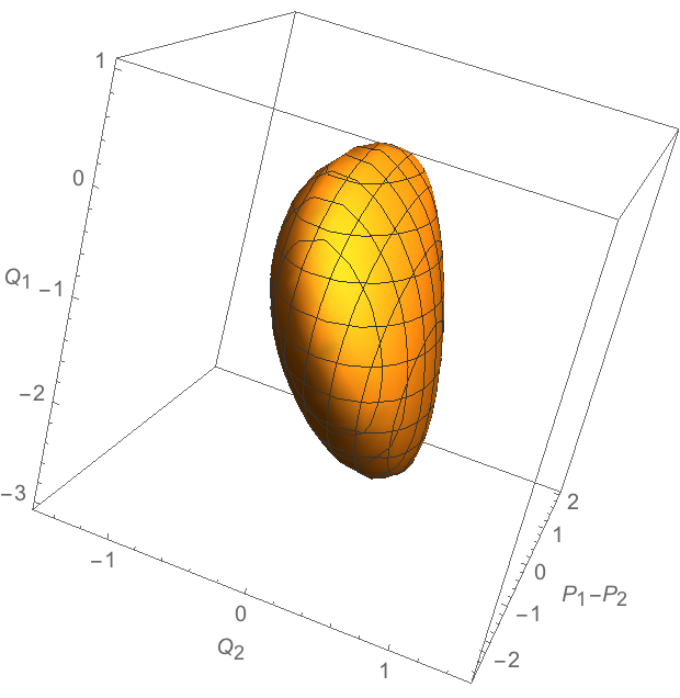
(a)

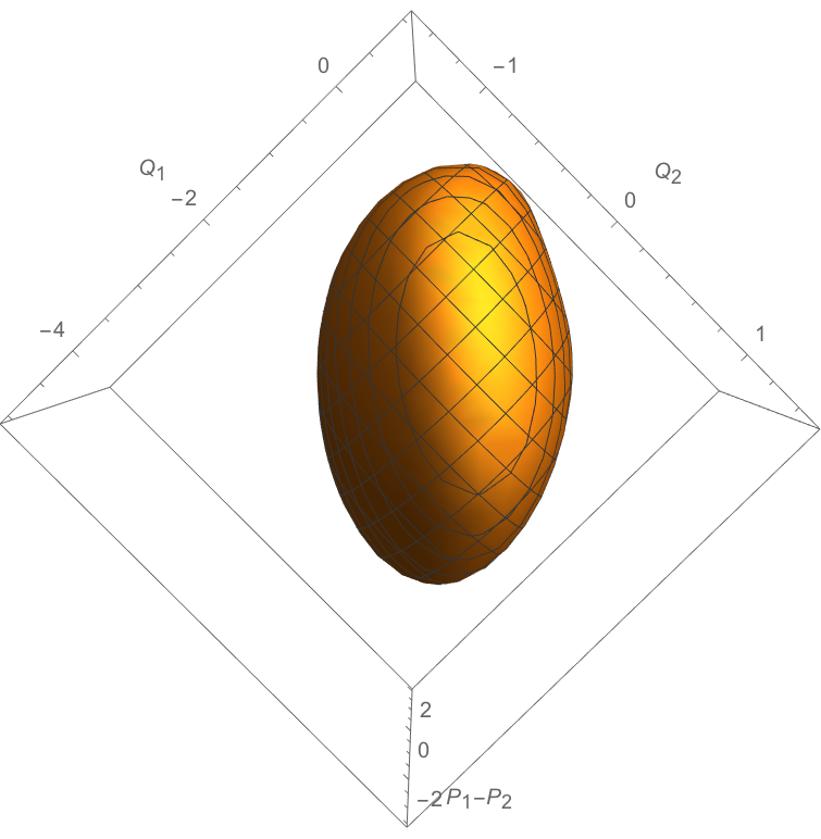
(b)

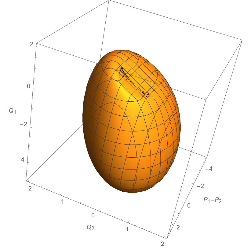
(c)

Figure 2: Projections of the full solvability set for the 3-bus model discussed in section III-B on the hyperplanes $P_{1}+P_{2}={\rm const}$. (a) $P_{1}+P_{2}=0$ and the projection is strongly convex. (b) $P_{1}+P_{2}=1/2$ and the projection develops a flat boundary i.e. it is convex but not strongly convex. (c) $P_{1}+P_{2}=1$ and the projection is visibly non-convex.

IV Convexity of Real Solvability Set

As we saw above the full solvability set of the unhomogeneous networks is generally non-convex. Nevertheless convexity often can be preserved if instead of the full solvability set one considers only the real solvability set – the solvability set of real powers. From the point of view of the underlying quadratic map, we restrict our consideration to $n$ real-valued quadratic functions, $P_{i}=\Re(S_{i})$, (5) of $n$ complex variables $V_{i}$. Hence in (8) we should take $m=n$ with $p,c\in{\mathbb{R}}^{n}$. In practice it is convenient to work with the full vectors $p=(P_{1},\dots,Q_{1},\dots)^{T}\in{\mathbb{R}}^{2n}$ and $c\in{\mathbb{R}}^{2n}$ but restrict $c_{i}=0$ for $i>n$. The same condition can be written as $\Im(\mathcal{C}_{i})=0$. Notice, that (19) satisfies this condition and therefore if all lines have non-zero resistance the associated quadratic map is definite. In what follows we will assume the latter, i.e. $\Re(y_{ik})>0$ for all $i\sim k$. In case some lines are purely reactive with $\Re(y_{ik})=0$, it is possible to add a small positive number $\epsilon$ to each such $y_{ik}$, establish convexity in that case and then take $\epsilon$ to zero. Since the convexity is stable property, this would grantee convexity for $\epsilon=0$ as well.

IV-A Convexity of acyclic networks

If the consideration is restricted to real powers, real solvability set of any radial (acyclic) network is convex. As in the case of full solvability set for homogeneous acyclic networks, section III-A, the idea of the proof would be to use Theorem 3.4 of [21].
Lemma 2. For a connected network with non-zero resistances $\Re(y_{ik})>0$ for all $i\sim k$, and vector $c\neq 0$, $\Im(\mathcal{C}_{i})=0$, such that $H_{c}\succeq 0$ all $\mathcal{C}_{i}>0$.
Proof. The proof is very similar to the proof of Lemma 1. The condition $H_{c}\succeq 0$ requires all diagonal elements of $H_{c}$ to be non-negative. Since all $\Re(y_{ik})$ are positive and $\mathcal{C}_{i}$ are real and can be brought outside of $\Re$, from (13) it follows that $\mathcal{C}_{i}\geq 0$ for all $i=1,\dots,n$. Now let us assume that $\mathcal{C}_{i}=0$ for a particular $i$. For $H_{c}$ to be positive semi-definite all elements $(H_{c})_{ik}$ must be zero, $(\mathcal{C}_{i}+\mathcal{C}_{k})y_{ik}=0$. This is only possible if $\mathcal{C}_{k}=0$ for all $k\sim i$. And since the network is connected, repeating this consideration enough times, we find $\mathcal{C}_{k}=0$ for all $k=1,\dots,n$. This contradicts the assumption $c\neq 0$, and therefore all $\mathcal{C}_{i}>0$.

Theorem 2. The real solvability set of any connected acyclic (with tree topology) network is convex.
Proof. As was explained in the beginning of this section, without loss of generality we can assume that $\Re(y_{ik})>0$ for any two connected nodes $i\sim k$. Then (19) and (20) establish that the corresponding quadratic map is convex. To apply the sufficient condition for convexity (I) we assume that number $a$ and $c\neq 0$, $\Im(\mathcal{C}_{i})=0$ are such that matrix $A$ of (27) is positive semi-definite. Using Lemma 2 for the submatrix $H_{c}$ of $A$ we readily find that all $\mathcal{C}_{i}$ are positive. From here it follows that matrix elements $(H_{c})_{ik}$ for any two connected nodes $i\sim k$ are non-zero,

$$\Re(H_{c})_{ik}=-(\mathcal{C}_{i}+\mathcal{C}_{j})\Re(y_{ik})<0\ .$$ (42)

Similarly for $i\sim 0$ vector element $(J_{c})_{i}$ also does not vanish,

$$\Re((J_{c})_{i})=\mathcal{C}_{i}\Re(y_{i0})>0\ .$$ (43)

Hence, matrix $A$ (27) has the topology of the network. For acyclic networks we can immediately apply Theorem 3.4 of [21] which finishes the proof.

IV-B Convexity of purely resistive networks

When the network is purely resistive $\Im(y_{ik})=0$ and $\Re(y_{ik})>0$ for $i\sim k$ the real solvability set is also convex for any network topology. The approach we take here to prove it is similar to the proof in the subsection 5.1 of [20] that the power solvability region for purely resistive DC model is convex. Notice however that in this paper we do not restrict voltages to be real, i.e. we consider an AC model of power flow with purely resistive connected network of arbitrary topology.
Theorem 3. The real solvability set of any connected purely resistive network is convex.
Proof. The idea of the proof is to use the sufficient condition for convexity (I). We start by using (19) and (20) to show that the associated quadratic map is definite. Next, we consider $c\neq 0$ with all $\mathcal{C}_{i}$ being real $\mathcal{C}_{i}$ such that $H_{c}\succeq 0$ and singular. Using Lemma 2 we find that all $\mathcal{C}_{i}$ are strictly positive. Let us consider a normalized vector $|{\bf V}_{\rm null}|=1$, ${\bf V}_{\rm null}\in{\mathbb{C}}^{n}$ which satisfies (22). This vector minimizes the following quadratic form

$${\bf V}^{\dagger}H_{c}{\bf V}=\sum_{i=1}^{n}(H_{c})_{ii}|V_{i}|^{2}-2\sum_{i\sim k}(\mathcal{C}_{i}+\mathcal{C}_{j})y_{ik}\Re(V_{i}^{*}V_{k})\ ,$$ (44)

subject to ${\bf V}^{\dagger}{\bf V}=1$. Taking into account that for any $i\sim k$ the combination $(\mathcal{C}_{i}+\mathcal{C}_{j})y_{ik}>0$, for the given values of $|V_{i}|$, the quadratic form (44) will be minimal if $\Re(V_{i}^{*}V_{k})=|V_{i}||V_{k}|$. Hence all components of ${\bf V}_{\rm null}$ minimizing (44) must have the same phase. Thus, without loss of generality we can assume that all components of ${\bf V}_{\rm null}$ are real and non-negative. Therefore

$$J_{c}^{\dagger}{\bf V}_{\rm null}=\sum_{i\sim 0}\mathcal{C}_{i}y_{i0}V_{i}\ ,$$ (45)

is a sum of non-negative terms. For the condition (23) to be satisfied, it would require $V_{i}=0$ for each node connected with the slack $i\sim 0$. Next, we write $i$-th component of the vector $H_{c}{\bf V}_{\rm null}=0$,

$$\mathcal{C}_{i}\sum_{k\sim i}y_{ik}V_{i}-\sum_{k\sim i}(\mathcal{C}_{i}+\mathcal{C}_{k})y_{ik}V_{k}/2=0\ .$$ (46)

Assuming $V_{i}=0$, since all $V_{k}$ are non-negative, the condition (22) can be only satisfied if $V_{k}=0$ at all nosed $k$ adjacent to $i$. Since the network is connected, by repeating this logic we find that all components of vector ${\bf V}_{\rm null}$ are zero, which contradicts the assumption that ${\bf V}_{\rm null}$ is normalized. Finally, we conclude that whenever $H_{c}\succeq 0$ and $c\neq 0$, the system of equations(22,23) is not feasible, the sufficient condition for convexity (I) applies and the real solvability set is convex.

V Conclusion

In this paper we have employed a novel geometric approach of [20] to establish convexity of power flow solvability sets for various typos of networks. For the distribution network with a radial topology, we established that the full solvability set consisting of real and reactive powers is convex whenever the network is homogeneous (Theorem 1). By considering a simple example of a radial 3-bus network we have demonstrated that the condition of the network to be homogeneous is crucial, once it is relaxed the full solvability set immediately ceases to be convex. Next, we considered the real solvability set, i.e. the solvability set consisting only of real powers, and established its convexity for an arbitrary distribution network with tree topology (Theorem 2). We have also shown that real solvability set is convex for a purely resistive network with arbitrary topology (Theorem 3).

Our results open a few new directions for research. First, it remains an open question to identify other network classes with convex solvability sets. For example, our preliminary studies suggest that a homogeneous distribution network with a ring topology ($n$ PQ-buses connected in a series with the first and the last connected to the slack) might have a convex full solvability set. Second, the approach of [20] allows to establish rigorous analytic bounds on the convex subset within the solvability set. Realistic networks may not satisfy all necessary conditions for the solvability set to be convex. Thus, transmission networks are often close to be homogeneous, but variations of the impedance to resistance ratio are always present. As was illustrated in section III-B this is still likely to be sufficient for the practically-relevant part of the solvability set to be convex. We leave it as an interesting problem for the future to derive analytic bounds similar to (40) for various types of networks.

Certification of solvability set convexity for realistic power grid would allow for application of many powerful algorithms available for convex domains. For example, for the purposes of robust power flow analysis, construction of inner approximations of secure operation regions could be accomplished by taking a convex hull of points on the solvability set boundary. While it is unlikely that global convexity can be established for realistic power cases, even semi-local convexity covering the realistic operating regions may be extremely helpful in development of next generation of power system decision-support tools.

References

- [1] F. D. Galiana. Power-voltage limitations imposed by the network structure of a power system. IEEE Conference on Power Industry Computer Applications (PICA), 1975, pp. 356-–363.
- [2] E. Hnyilicza, S.T. Lee, F.C. Schweppe. Steady-state security regions: The set theoretic approach. IEEE Conference on Power Industry Computer Applications (PICA), 1975, pp. 347-–355.
- [3] Hiskens I.A., Davy R.J. Exploring the power flow solution space boundary. IEEE transactions on power systems. 2001 Aug;16(3):389-95.
- [4] B. Lesieutre, I. Hiskens. Convexity of the set of feasible injections and revenue adequacy in FTR markets. IEEE Transactions on Power Systems, 20 (5), 2005, pp. 1790–1798
- [5] Y. Makarov, Z. Dong, D. Hill. On convexity of power flow feasibility boundary. IEEE Transactions on Power Systems, 23 (2), 2008 pp. 811–813
- [6] Lavaei J, Low SH. Zero duality gap in optimal power flow problem. IEEE Transactions on Power Systems. 2012 Feb;27(1):92–107.
- [7] Lesieutre, B. C., Molzahn, D. K., Borden, A. R., and DeMarco, C. L. (2011, September). Examining the limits of the application of semidefinite programming to power flow problems. In Communication, Control, and Computing (Allerton), 2011 49th Annual Allerton Conference on (pp. 1492-1499). IEEE.
- [8] Lavaei J, Low SH. Convexification of optimal power flow problem. In Communication, Control, and Computing (Allerton), 2010 48th Annual Allerton Conference on 2010 Sep 29 (pp. 223–232). IEEE.
- [9] Gan L, Li N, Topcu U, Low SH. Optimal power flow in tree networks. InDecision and Control (CDC), 2013 IEEE 52nd Annual Conference on 2013 Dec 10 (pp. 2313–2318). IEEE.
- [10] Gan L, Li N, Topcu U, Low SH. Exact convex relaxation of optimal power flow in radial networks. IEEE Transactions on Automatic Control. 2015 Jan;60(1):72–87.
- [11] Low SH. Convex relaxation of optimal power flow, Part I: Formulations and equivalence. IEEE Transactions on Control of Network Systems. 2014 Mar;1(1):15–27.
- [12] Low SH. Convex relaxation of optimal power flow, Part II: Exactness. IEEE Transactions on Control of Network Systems. 2014 Jun;1(2):177–89.
- [13] Low SH. Convex relaxation of optimal power flow: A tutorial. InBulk Power System Dynamics and Control-IX Optimization, Security and Control of the Emerging Power Grid (IREP), 2013 IREP Symposium 2013 Aug 25 (pp. 1–15). IEEE.
- [14] Bose S, Gayme DF, Chandy KM, Low SH. Quadratically constrained quadratic programs on acyclic graphs with application to power flow. IEEE Transactions on Control of Network Systems. 2015 Sep;2(3):278–87.
- [15] Zhang B, Tse D. Geometry of feasible injection region of power networks. InCommunication, Control, and Computing (Allerton), 2011 49th Annual Allerton Conference on 2011 Sep 28 (pp. 1508-1515). IEEE.
- [16] Zhang B, Tse D. Geometry of injection regions of power networks. IEEE Transactions on Power Systems. 2013 May;28(2):788–97.
- [17] Lavaei J, Tse D, Zhang B. Geometry of power flows in tree networks. InPower and Energy Society General Meeting, 2012 IEEE 2012 Jul 22 (pp. 1–8). IEEE.
- [18] Lavaei J, Tse D, Zhang B. Geometry of power flows and optimization in distribution networks. IEEE Transactions on Power Systems. 2014 Mar;29(2):572–83.
- [19] Dymarsky A. Convexity of a small ball under quadratic map. Linear Algebra and its Applications. 2016 Jan 1;488:109–23.
- [20] Dymarsky A. On the convexity of image of a multidimensional quadratic map. arXiv:1410.2254.
- [21] van der Holst H. Graphs whose positive semi-definite matrices have nullity at most two. Linear Algebra and its Applications. 2003 Dec 1;375:1–1.