Electrical Impedance Tomography with Restricted Dirichlet-to-Neumann Map Data

Abstract

We propose a new numerical method to reconstruct the isotropic electrical conductivity from measured restricted Dirichlet-to-Neumann map data in electrical impedance tomography (EIT) model. ”Restricted Dirichlet-to-Neumann (DtN) map data” means that the Dirichlet and Neumann boundary data for EIT are generated by a point source running either along an interval of a straight line or along a curve located outside of the domain of interest. We “convexify” the problem via constructing a globally strictly convex Tikhonov-like functional using a Carleman Weight Function. In particular, two new Carleman estimates are established. Global convergenceto the correct solution of the gradient projection method for this functional is proven. Numerical examples demonstrate a good performance of this numerical procedure.

2010 Mathematics Subject Classification: 35R30.

1 Introduction

We develop in this paper a new globally convergent numerical method of the reconstruction of the internal electrical conductivity in the inverse problem of Electrical Impedance Tomography (EIT). The main part of the paper is devoted to the theory of this method. Next, numerical examples are presented. A general analytical concept of this method was originally proposed in the work [31] of the first author. However, it was not sufficiently specified in [31] for the EIT case. Unlike the conventional case of the Dirichlet-to-Neumann map (DtN) boundary data, it was proposed in [31] to use the so-called “restricted DtN map data” on the boundary. In the case of restricted DtN data, the number $d=2,3$ of free variables in the data equals the number of free variables in the unknown conductivity coefficient in the $\mathbb{R}^{d}$ case. We achieve this via truncation of a Fourier-like series. Note that the conventional DtN requires $m=4$ of free variables in the data in the 3D case.

Any Coefficient Inverse Problem (CIP) is highly nonlinear and ill-posed. As a result, a conventional least squares Tikhonov functional for a CIP is non-convex. The latter means that, as a rule, that functional has many local minima and ravines, see, e.g. [37] for a good numerical example. Hence, to obtain a good approximation for the exact solution of a CIP, one should start iterations of the minimization method for this functional in a small neighborhood of the exact solution. We call this local convergence. However, it is often unclear how to practically obtain such a good first guess.

Unlike the conventional case, we “convexify” the problem. More precisely, we construct a weighted Tikhonov-like functional with the Carleman Weight Function (CWF) in it. The CWF is the function which is involved in the Carleman estimate for the Laplace operator. The presence of the CWF ensures the strict convexity of this functional on any a priori chosen ball of an arbitrary radius $R>0$ in an appropriate Hilbert space. The latter guarantees the global convergence of the gradient projection method of the optimization of this functional to the exact solution of the original inverse EIT problem. We call a numerical method for a CIP globally convergent if there is a theorem, which guarantees that this method delivers at least one point in a sufficiently small neighborhood of the exact solution of that CIP without any advanced knowledge of this neighborhood. The size of this neighborhood should depend on measurement and approximation errors. The numerical method of this paper converges globally.

Electrical impedance tomography (EIT) is a non invasive and diffusive imaging method to recover the electrical conductivity distribution inside an object of interest by using the DtN map on the boundary. This modality is safe, portable and also has many clinical imaging applications [18]. There is a vast number of research papers discussing EIT. It has been analytically proven that the interior electrical conducting is uniquely determined by the Dirichlet-to-Neumann map on the boundary [12, 36, 40]. However, the EIT inverse problem is essentially ill-posed compared with other imaging modalities in practice [11], since the DtN data on the boundary is not that sensitive to the conductivity change inside the domain of interest.

In the past three decades, there were numerous studies on the EIT imaging method with quite many publications. Since this paper is not a survey of EIT, we now provide a far incomplete list of references on this topic. The recovery of small inclusions from boundary measurements is discussed in [3, 32]. Hybrid conductivity imaging methods are presented in [4, 39, 42]. The multi-frequency EIT imaging methods are discussed in [2, 38]. In particular, [2] also shows that the frequency difference method can eliminate the modeling errors. Both the finite element method and the adaptive finite element method are also applied to recover the internal conductivity [21, 35]. The imaging algorithms based on the sparsity reconstruction are considered in [2, 20]. In [17] a globally convergent method for shape reconstruction in EIT is proposed. Siltanen and Mueller have done a lot work on the EIT inverse problem, including d-bar method, diction reconstruction method, recovering boundary shape and imaging the anisotropic electrical conductivity [1, 13, 16, 15]. Hyvonen, P$\ddot{a}$iv$\ddot{a}$rinta and Tamminen also offer in their recent paper a new way to solve EIT problem [19].

In a typical EIT experiment, constant electrical currents are applied to the electrodes on the boundary of the object to image. Then the electrical potentials are measured on the boundary. This gives the DtN map data. The EIT problem is to recover the internal electric conductivity from these DtN measurements. This problem is essentially ill-posed.

Unlike the DtN, by our definition, restricted DtN data means that the Dirichlet and Neumann boundary data for the EIT problem are generated by a point source running either along an interval of a straight line or along a curve located outside of the domain to be imaged. Moreover, the restricted DtN data can be given either on the whole or on a part of the boundary.

The key element of our method consists in the construction of a weighted Tikhonov-like functional which is strictly convex on any a priori chosen ball of an arbitrary radius $R>0$ in an appropriate Hilbert space. In other words, we “convexify” the problem. The main ingredient of that Tikhonov-like functional is the presence of the CWF in it. If the exact solution belongs to that ball (as it should be assumed in the framework of the regularization theory [41]), then convergence of the gradient projection method to the exact solution is guaranteed if starting from an arbitrary point of this ball. Hence, this is global convergence. On the other hand, recall that convergence of a gradient-like method to the exact solution for a non-convex functional might be guaranteed only if its starting point is located in a small neighborhood of this solution.

Carleman estimates were introduced in the field of Coefficient Inverse Problems (CIPs) in the work [10]. There are many works devoted to the method of [10], see, e.g. the survey [23], the most recent book [9] and the references cited therein. The goal of the authors of [10] was to prove global uniqueness and stability results for CIPs. Later, however, it became clear that Carleman estimates can also be applied to numerical methods for some ill-posed problems for PDEs. First, CWFs can be applied to convexify CIPs, see [8, 22, 27] for the theory and [6, 26, 29, 30] for both the theory and numerical results. Second, CWFs can be applied to prove convergence of the so-called quasi-reversibility method for ill-posed Cauchy problems for linear PDEs [24]. Third, CWFs are applicable for the convexification of some ill-posed Cauchy problems for quasilinear PDEs, see [25] for the theory and [5, 28] for both the theory and numerical results.

However, in the above cited works on the convexification for CIPs only the case of a single location of the source was considered for either time dependent or frequency dependent data. Unlike the above cited publications, in [31] a significantly new convexification method was proposed. This was done for the case when the boundary data for a CIP are generated by a point source which is running along an interval of a straight line. The resulting boundary data form the above mentioned restricted DtN. In this work we specify the idea of [31] for the case of an inverse problem for EIT with the restricted DtN data.

To minimize the above mentioned weighted Tikhonov-like functional, we propose a multi-level method, which is somewhat similar with the adaptivity method, see, e.g. [7] for a detailed theory of the adaptivity. However, we do not extend to our case the theory of the adaptivity presented in [7], i.e. we restrict our attention only to the numerical aspect of the adaptivity. Thus, we minimize that functional on a coarse mesh first and use the solution achieved on the coarse mesh (first level) as the starting point for a finer mesh (second level). We repeat this process until we get a solution on $K_{th}$ level. We have found that we get a rough image on the coarse mesh (e.g. support, shape) of the internal conductivity much faster than on a finer mesh, while on the finer mesh with the starting point from the solution on the coarse mesh, the solution is corrected in details (e.g., amplitude and shape).

2 EIT with restricted Dirichlet-to-Neumann (DtN) data

All functions below are real valued ones. The same is about functional spaces, including Hilbert spaces.

2.1 Model

In this section, we formulate the restricted DtN for the inverse EIT problem. First, we recall the traditional DtN for EIT. Let $\Omega$ be an open bounded domain in $\mathbb{R}^{d}$ ($d=2,3$) to be imaged with a smooth boundary $\partial\Omega$. The EIT forward problem is formulated as: For any given input current

$$g_{1}\in L_{0}^{2}(\partial\Omega):=\{g\in L^{2}(\Omega):\int_{\partial\Omega}g\,ds=0\}$$

and the conductivity distribution $\sigma(x)$, find the function $u(x)\in H^{1}(\Omega)$ such that

(1) $$\left\{\begin{aligned} -\nabla\cdot(\sigma(x)\nabla u(x))&=0\quad\mbox{ in }\Omega,\\ \sigma(x)\frac{\partial u}{\partial\nu}&=g_{1}(x)\quad\mbox{on }\partial\Omega,\\ \int_{\partial\Omega}u(x)\,ds&=0,\end{aligned}\right.$$

where $\nu$ is the outward unit normal vector on $\partial\Omega$. Denote $g_{0}(x)=u|_{\partial\Omega}$. Then the inverse EIT problem is to recover the internal conductivity function $\sigma(x)$ from the DtN map $\Lambda:g_{0}\rightarrow g_{1}$.

In this paper, we consider the EIT problem with the source outside the domain of interest and the restricted DtN data measured on the boundary of the domain of interest, as described below.

To avoid working with singularities and also to simplify the presentation, we model the point source here by a $\delta-$like function instead of the $\delta-$function. Let $\varepsilon>0$ be a sufficiently small number. Let the source function $f(x)$ be such that

(2) $$f(x)\in C^{\infty}(\mathbb{R}^{n}),f(0)\neq 0,f(x)\geq 0,\forall x\in\mathbb{R}^{d},\text{ }f(x)=0\text{ for }|x|>\varepsilon.$$

Let $G\subset\mathbb{R}^{n}$ be a bounded domain with its boundary $\partial G\in C^{1}$, $\Omega\subset G$ and $\partial\Omega\cap\partial G=\varnothing$. Let $\overline{x}\in\mathbb{R}^{d-1}$ be a fixed point. For $s\in[0,1]$ denote $x_{s}=\left(x_{1s},\overline{x}\right)$ the position of the point source. Let $I=\{x_{s}=\left(x_{1s},\overline{x}\right):s\in[0,1]\}$ be the interval of the straight line $\left\{x=\left(x_{1},\overline{x}\right),x_{1}\in\mathbb{R}\right\}.$ Let $I_{\varepsilon}=\{x\in\mathbb{R}^{d}:dist(x,I)<\varepsilon\}$, where $dist(x,I)$ is the Hausdorff distance between the point $x$ and the set $I$. We also assume that $I_{\varepsilon}\subset(G\setminus\overline{\Omega}),$ which means that the support of the source function is outside of the domain $\Omega$.

Let the function

(3) $$\sigma\left(x\right)\in C^{2+\alpha}(\overline{G}),\sigma\left(x\right)=1\text{ for }x\in G\setminus{\Omega}\text{ and }\sigma\left(x\right)\geq\sigma_{0}=const.>0.$$

Here $\alpha=const.\in\left(0,1\right)$ and $C^{k+\alpha}(\overline{G})$ be the Hölder space, where $k\geq 0$ is an integer. Assume first that $\sigma(x)$ is known. For each source position $x_{s}\in I$ we define the forward boundary value problem for EIT as the problem of finding the function $u(x,s)$ such that

(4) $$\left\{\begin{array}[]{lll}\nabla\cdot(\sigma(x)\nabla u(x,s))&=-f(x-x_{s}),&\qquad x\in G,\forall x_{s}\in\overline{I}\\ u(x,s)|_{x\in\partial G}&=0,&\qquad\forall x_{s}\in\overline{I}.\end{array}\right.$$

It is well known that for each $x_{s}\in I$ the problem (4) has unique solution

(5) $$u(x,s)\in C^{3+\alpha}(\overline{G}),\forall x_{s}\in\overline{I},$$

see, e.g. [14]. We measure both Dirichlet and Neumann boundary conditions of the function $u$ on a part $\Gamma\subseteq\partial\Omega$ of the boundary $\partial\Omega$,

(6) $$u(x,s)|_{x\in\Gamma,x_{s}\in\overline{I}}=g_{0}(x,s)\text{ and }\partial_{\nu}u(x,s)|_{x\in\Gamma,x_{s}\in\overline{I}}=g_{1}(x,s).$$

We call the Dirichlet and Neumann boundary data (6)  “restricted DtN data”.

If the coefficient $\sigma(x)$ is known, then, having the solution of the forward problem (4), one can easily compute functions $g_{0}(x,s)$ and $g_{1}(x,s).$  Suppose now that the function $\sigma(x)$ is unknown. Then we arrive at the following inverse problem:

Coefficient Inverse Problem (CIP). Assume that the function $\sigma\left(x\right)$ is unknown for $x\in\Omega$ and also that conditions (2), (3) hold. Also, assume that functions $g_{0}(x,s)$ and $g_{1}(x,s)$ in (6) are known for all $x\in\Gamma,x_{s}\in\overline{I}.$ Determine the function $\sigma\left(x\right).$

Note that in this CIP the number $d$ of free variables in the data equals the number of free variables in the unknown coefficient.

2.2 An equivalent problem

In this subsection, we transform the above CIP to an inverse problem for a quasilinear PDE. First, introduce the well known change of variables

(7) $$u_{1}=\sqrt{\sigma}u,$$

where $u(x,s)$ is the solution of problem (4). Then

(8) $$\left\{\begin{array}[]{lll}\Delta u_{1}(x,s)+a_{0}(x)u_{1}(x,s)&=-f(x-x_{s}),&\qquad\forall x_{s}\in\overline{I},\\ u_{1}(x,s)|_{x\in\partial G}&=0,&\qquad\forall x_{s}\in\overline{I},\end{array}\right.$$

where

(9) $${a_{0}(x)=-\frac{\Delta\left(\sqrt{\sigma(x)}\right)}{\sqrt{\sigma(x)}}}.$$

Recalling that $\sigma=1$ on $\partial\Omega,$ we obtain from (6)

(10) $$u_{1}(x,s)|_{x\in\Gamma,s\in[0,1]}=g_{0}(x,s)\text{ and }\partial_{n}u_{1}(x,s)|_{x\in\Gamma,s\in[0,1]}=g_{1}(x,s).$$

If we would recover the function $a_{0}(x)$ for $x\in\Omega$ from conditions (8), (10), then, assuming that $0$ is not an eigenvalue of the elliptic operator $\Delta+a_{0}\left(x\right)$ with the Dirichlet boundary condition either on $\partial\Omega$ or on $\partial G,$ we would recover the function $\sigma\left(x\right)$ via solving elliptic equation (9) either in the domain $\Omega$ with the Dirichlet boundary condition $\sigma\mid_{\partial\Omega}=1,$ or in the domain $G$ with the Dirichlet boundary condition $\sigma\mid_{\partial G}=1.$ Hence, we focus below on the recovery of the function $a_{0}(x)$ for $x\in\Omega$ from conditions (8), (10).

It follows from (2), (4), (7) and the maximum principle for elliptic equations [14] that $u_{1}(x,s)>0$ for all $x\in\overline{\Omega}$ and all $s\in\left[0,1\right].$ Hence, we can consider the function $v(x,s),$

(11) $$v(x,s)=\ln u_{1}(x,s).$$

Then $u_{1}(x,s)=e^{v(x,s)}$ and (8) implies that

(12) $$\Delta v(x,s)+\left(\nabla v(x,s)\right)^{2}=-a_{0}(x),\qquad x\in\Omega,\forall s\in[0,1].$$

Here we use (2) and the fact that $I_{\varepsilon}\subset(G\setminus\overline{\Omega})$. In addition, using (10), we obtain

(13) $$v(x,s)|_{x\in\Gamma,s\in[0,1]}=\tilde{g}_{0}(x,s)\text{ and }\partial_{\nu}v(x,s)|_{x\in\Gamma,s\in[0,1]}=\tilde{g}_{1}(x,s),$$

where

$$\tilde{g}_{0}(x,s)=\ln g_{0}(x,s)\text{ and }\tilde{g}_{1}(x,s)=\frac{g_{1}(x,s)}{g_{0}(x,s)}.$$

Differentiating equation (12) with respect to $s$ and noting that the function $a_{0}(x)$ is independent on $s$, we obtain

(14) $$\Delta v_{s}+2\nabla v_{s}\cdot\nabla v=0,\qquad x\in\Omega,\forall s\in[0,1].$$

Now the above CIP is reduced to the following problem:

Reduced Problem. Recover the function $v\left(x,s\right)$ from equations (14), given the boundary measurements $\tilde{g}_{0}(x,s)$ and $\tilde{g}_{1}(x,s)$ in (13).

If the function $v\left(x,s\right)$ is approximated, then the approximate coefficient $a_{0}(x)$ can be found via (12). Thus, our focus below is on the solution of Reduced Problem.

3 Cauchy problem for a system of coupled quasilinear elliptic equations

To solve Reduced Problem, we obtain in this section a system of coupled quasilinear elliptic equations.

3.1 A special orthonormal basis in $L^{2}\left(0,1\right)$

Let $\left(,\right)$ denotes the scalar product in $L^{2}\left(0,1\right).$ We need to construct such an orthonormal basis in the space $L^{2}\left(0,1\right)$ of real valued functions $\left\{\psi_{n}\left(s\right)\right\}_{n=0}^{\infty}$ that the following two conditions are met:

1. $\psi_{n}\in C^{1}\left[0,1\right],$ $\forall n=0,1,...$

2. Let $a_{mn}=\left(\psi_{n}^{\prime},\psi_{m}\right).$ Then the matrix $M_{k}=\left(a_{mn}\right)_{m,n=0}^{k-1}$ should be invertible for any $k=1,2,...$

Neither the basis of any type of classical orthonormal polynomials nor the basis of trigonometric functions $\left\{\sin\left(2\pi ns\right),\cos\left(2\pi ns\right)\right\}_{n=0}^{\infty}$ do not satisfy the second condition. Indeed, in either of these cases all elements of the first raw of the matrix $M_{k}$ would be equal to zero. The required basis was constructed in [31]. We now briefly describe this construction for the convenience of the reader.

Consider the set of functions $\left\{s^{n}e^{s}\right\}_{n=0}^{\infty}.$ This set is complete in $L^{2}\left(0,1\right).$ We orthonormalize it using the classical Gram-Schmidt orthonormalization procedure. We start from $n=0$, then take $n=1$, etc. Then we obtain the orthonormal basis $\left\{\psi_{n}\left(s\right)\right\}_{n=0}^{\infty}$ in $L^{2}\left(0,1\right).$ Each function $\psi_{n}\left(s\right)$ has the form

(15) $$\psi_{n}\left(s\right)=P_{n}\left(s\right)e^{s},$$

where $P_{n}\left(s\right)$ is the polynomial of the degree $n$. Hence, one can say that these polynomials are orthogonal to each other in the weighted $L^{2}\left(0,1\right)$ space with the weight function $e^{2s}.$ Lemma 3.1 ensures that the above property number 2 holds for functions $\psi_{n}\left(s\right)$.

Lemma 3.1 [31]. We have

(16) $$a_{mn}=\left[\psi_{n}^{\prime},\psi_{m}\right]=\left\{\begin{array}[]{c}1\text{ if }n=m,\\ 0\text{ if }n<m.\end{array}\right.$$

For an integer $k\geq 1$ consider the $k\times k$ matrix $M_{k}=\left(a_{mn}\right)_{\left(m,n\right)=\left(0,0\right)}^{\left(k-1,k-1\right)}.$ Then (16) implies that $M_{k}$ is an upper diagonal matrix and $\det\left(M_{k}\right)=1.$ Thus, the inverse matrix $M_{k}^{-1}$ exists.

3.2 Cauchy problem for a system of coupled quasilinear elliptic equations

Fix an integer $N\geq 1.$ Denote $\Psi\left(N\right)=\left\{\psi_{n}\left(s\right)\right\}_{n=0}^{N-1}.$ We assume that the function $v\left(x,s\right)$ in (11) can be represented via the truncated Fourier-like series with respect to the orthonormal basis of functions $\psi_{n}\left(s\right)$ in (15),

(17) $$v\left(x,s\right)=\mathop{\displaystyle\sum}\limits_{n=0}^{N-1}v_{n}\left(x\right)\psi_{n}\left(s\right),\text{ }x\in\Omega,\forall s\in[0,1].$$

Then the derivative $v_{s}\left(x,s\right)$ is

(18) $$v_{s}\left(x,s\right)=\mathop{\displaystyle\sum}\limits_{n=0}^{N\_1}v_{n}\left(x\right)\psi_{n}^{\prime}\left(s\right),\text{ }x\in\Omega,\forall s\in[0,1].$$

Note that functions $v_{n}\left(x\right)$ are unknown and should be determined. By (5) and (7) it is reasonable to assume that functions $v_{n}\left(x\right)$ are such that

(19) $$v_{n}\in C^{3}\left(\overline{\Omega}\right),n=0,...,N-1.$$

It is likely that (19) can be proven using the classical theory of elliptic PDEs  [14]. However, we are not doing this here for brevity.

Substituting (17) and (18) in (14), we obtain

(20) $$\mathop{\displaystyle\sum}\limits_{n=0}^{N-1}\Delta v_{n}\left(x\right)\psi_{n}^{\prime}\left(s\right)+\mathop{\displaystyle\sum}\limits_{n,k=0}^{N-1}\nabla v_{n}\left(x\right)\nabla v_{k}\left(x\right)\psi_{n}^{\prime}\left(s\right)\psi_{k}\left(s\right)=0,\text{ }x\in\Omega,\forall s\in[0,1].$$

Consider the vector function of unknown coefficient $v_{n}\left(x\right)$ in the expansion (17),

(21) $$V\left(x\right)=\left(v_{0}\left(x\right),...,v_{N-1}\left(x\right)\right)^{T}.$$

For $m=0,...,N-1$ multiply both sides of (20) by the function $\psi_{m}\left(s\right)$ and then integrate with respect to $s\in\left(0,1\right).$ Using (19) and (21), we obtain

(22) $$M_{N}\Delta V-\widetilde{F}\left(\nabla V\right)=0,\text{ }x\in\Omega,V\in C^{3}\left(\overline{\Omega}\right),$$

where the $N-$dimensional vector function $\widetilde{F}$ is quadratic with respect to the first derivatives $\partial_{x_{j}}v_{k}\left(x\right),j=1,..,d;k=0,...,N-1.$ Multiplying both sides of (22) by the inverse matrix $M_{N}^{-1}$ (Lemma 3.1), we obtain a system of coupled quasilinear elliptic equations,

(23) $$\Delta V-F\left(\nabla V\right)=0,x\in\Omega,V\in C^{3}\left(\overline{\Omega}\right),$$

(24) $$F\left(\nabla V\right)=M_{N}^{-1}\widetilde{F}\left(\nabla V\right).$$

Since the vector function $\widetilde{F}$ is quadratic with respect to the first derivatives $\partial_{x_{j}}v_{k}\left(x\right),$ then (24) implies that the vector function $F$ is also quadratic. In addition, using (13), we obtain Cauchy data for the vector function $V\left(x\right)$ on $\Gamma,$

(25) $$V\left(x\right)\mid_{\Gamma}=p_{0}\left(x\right),\partial_{\nu}V\left(x\right)\mid_{\Gamma}=p_{1}\left(x\right).$$

If we would solve the Cauchy problem (23), (25), then we would find coefficients $v_{n}\left(x\right)$ in (17). Next, we would substitute (17) in (12) and obtain the following approximate formula for the function $a_{0}\left(x\right):$

(26) $$a_{0}\left(x\right)=-\mathop{\displaystyle\sum}\limits_{n=0}^{N-1}\Delta v_{n}\left(x\right)\psi_{n}\left(s\right)+\left(\mathop{\displaystyle\sum}\limits_{n=0}^{N-1}\nabla v_{n}\left(x\right)\psi_{n}\left(s\right)\right)^{2},\text{ }x\in\Omega,s\in\left(0,1\right).$$

As to the value of the parameter $s$ for which the function $a_{0}\left(x\right)$ should be calculated in (26), it should be chosen numerically, similarly with [26, 29, 30]. Hence, we develop below a numerical method for solving problem (23), (25).

3.3 Two new Carleman estimates

Since in our numerical examples the domain $\Omega\subset\mathbb{R}^{2}$ is a disk, we prove in this subsection a new Carleman estimate for the Laplace operator, which is specifically used for the disk in the 2D case and for the ball in the 3D case. We work with the case when $\Gamma=\partial\Omega$ since this is done in our numerical experiments. In principle, Carleman estimates are known for this kind of domains, see, e.g. [22]. However, the CWF in [22] has a rather complicated form and changes too rapidly. On the other hand, the previous numerical experience of the first author with the convexification for CIPs [26, 29, 30] tells us that one should use a CWF of the simplest possible form, also, see, e.g. [6] for a similar statement. This is the reason of presenting here the Carleman estimate with a simple CWF which was not used before.

3.3.1 The 3D case

We derive in this section a new Carleman estimate for the 3D case when the domain $\Omega$ is a ball of the radius $\rho$,

(27) $$\Omega=\left\{x\in\mathbb{R}^{3}:\left|x\right|<\rho\right\}.$$

Let $\mu\in\left(0,\rho\right)$ be a number. Define the domain $\Omega_{\mu}$ as

(28) $$\Omega_{\mu}=\left\{x\in\mathbb{R}^{3}:\mu<\left|x\right|<\rho\right\}\subset\Omega.$$

Consider spherical coordinates

$$r=\left|x\right|\in\left(\mu,\rho\right),\varphi\in\left(0,2\pi\right),\theta\in\left(0,\pi\right),$$

$$x_{1}=r\cos\varphi\sin\theta,x_{2}=r\sin\varphi\sin\theta,x_{3}=r\cos\theta.$$

Also, denote

$$S_{\rho}=\left\{r=\rho\right\},S_{\mu}=\left\{r=\mu\right\}.$$

The Laplace operator in the spherical coordinates is

(29) $$\Delta_{\text{sp}}w=w_{rr}+\frac{1}{r^{2}\sin^{2}\theta}w_{\varphi\varphi}+\frac{1}{\sin\theta}\frac{\partial}{\partial\theta}\left(\sin\theta w_{\theta}\right)+\frac{2}{r}w_{r}=\widehat{\Delta}_{\text{sp}}w+\frac{2}{r}w_{r},$$

(30) $$\widehat{\Delta}_{\text{sp}}w=w_{rr}+\frac{1}{r^{2}\sin^{2}\theta}w_{\varphi\varphi}+\frac{1}{r^{2}\sin\theta}\frac{\partial}{\partial\theta}\left(\sin\theta w_{\theta}\right),$$

for an arbitrary function $w\in C^{2}\left(\overline{\Omega}_{\mu}\right)$. We single out the operator $\widehat{\Delta}_{\text{sp}}$ in (29), (30) since any Carleman estimate is independent on the low order derivatives of an operator, and also since we work in $\Omega_{\mu}$ where $r>\mu>0.$ Everywhere below $C=C\left(\Omega_{\mu}\right)>0$ denotes different constants depending only on the domain $\Omega_{\mu}.$ Let

$$\nabla w=\left(w_{x_{1}},w_{x_{2}},w_{x_{3}}\right)^{T}\text{ and }\nabla_{\text{sp}}w=\left(w_{r},\frac{w_{\varphi}}{r\sin\theta},\frac{w_{\theta}}{r}\right)^{T}.$$

Note that since $w_{\varphi}=-w_{x_{1}}\sin\varphi\sin\theta+w_{x_{2}}\cos\varphi\sin\theta,$ then the function $w_{\varphi}/\sin\theta$ does not have a singularity. It is well known that

(31) $$\left|\nabla w\right|\leq C\left|\nabla_{\text{sp}}w\right|\text{ in }\overline{\Omega}_{\mu},$$

(32) $$\left|\nabla_{\text{sp}}w\right|\leq C\left|\nabla w\right|\text{ in }\overline{\Omega}_{\mu}.$$

Introduce the subspace $H_{0}^{m}\left(\Omega_{\mu}\right)$ of the Hilbert space $H^{m}\left(\Omega_{\mu}\right)$ as

$$H_{0}^{m}\left(\Omega_{\mu}\right)=\left\{u\in H^{m}\left(\Omega_{\mu}\right):u\mid_{S_{\rho}}=u_{r}\mid_{S_{\rho}}=0\right\},\text{ }m=2,3.$$

We include the term with $\left(\Delta w\right)^{2}$ in the right hand side of the Carleman estimate (33) since we will need to estimate not only convergence for the vector function $W\left(x\right)$ (Theorem 5.4), but also to estimate convergence for the target coefficient $a_{0}(x)$ (Theorem 5.5). To do the latter, we will need to use equation (12) in which the Laplace operator is involved.

Theorem 3.1 (Carleman estimate). There exists a number $\lambda_{0}=\lambda_{0}\left(\Omega_{\mu}\right)\geq 1$ and a number $C=C\left(\Omega_{\mu}\right)>0,$ both depending only on the domain $\Omega_{\mu},$ such that for any function $w\in H^{2}\left(\Omega_{\mu}\right)$ and for all $\lambda\geq\lambda_{0}$ the following Carleman estimate with the CWF $e^{2\lambda r}$ holds:

(33) $$\mathop{\displaystyle\int}\limits_{\Omega_{\mu}}\left(\Delta w\right)^{2}e^{2\lambda r}dx\geq\frac{1}{2}\mathop{\displaystyle\int}\limits_{\Omega_{\mu}}\left(\Delta w\right)^{2}e^{2\lambda r}dx+C\lambda\mathop{\displaystyle\int}\limits_{\Omega_{\mu}}\left(\nabla w\right)^{2}e^{2\lambda r}dx+C\lambda^{3}\mathop{\displaystyle\int}\limits_{\Omega_{\mu}}w^{2}e^{2\lambda r}dx$$

$$-C\lambda e^{2\lambda\rho}\mathop{\displaystyle\int}\limits_{S_{\rho}}w_{r}^{2}dS-C\lambda^{3}e^{2\lambda\rho}\mathop{\displaystyle\int}\limits_{S_{\rho}}w^{2}dS-C\lambda^{3}e^{2\lambda\mu}\left\|w\right\|_{H^{2}\left(\Omega_{\mu}\right)}^{2}.$$

In particular, if $w\in H_{0}^{2}\left(\Omega_{\mu}\right),$ then

(34) $$\mathop{\displaystyle\int}\limits_{\Omega_{\mu}}\left(\Delta w\right)^{2}e^{2\lambda r}dx\geq\frac{1}{2}\mathop{\displaystyle\int}\limits_{\Omega_{\mu}}\left(\Delta w\right)^{2}e^{2\lambda r}dx+C\lambda\mathop{\displaystyle\int}\limits_{\Omega_{\mu}}\left(\nabla w\right)^{2}e^{2\lambda r}dx+C\lambda^{3}\mathop{\displaystyle\int}\limits_{\Omega_{\mu}}w^{2}e^{2\lambda r}dx$$

$$-C\lambda^{3}e^{2\lambda\mu}\left\|w\right\|_{H^{2}\left(\Omega_{\mu}\right)}^{2}.$$

Proof. We assume that $w\in C^{2}\left(\overline{\Omega}_{\mu}\right)$ since the case $w\in H^{2}\left(\Omega_{\mu}\right)$ can be handled automatically later via density arguments. Introduce the new function $q=we^{\lambda r}.$ Then

$$w=qe^{-\lambda r},w_{rr}=\left(q_{rr}-2\lambda q_{r}+\lambda^{2}q\right)e^{-\lambda r}.$$

By (30)

$$\left(\widehat{\Delta}_{\text{sp}}w\right)^{2}e^{2\lambda r}r\sin\theta=\left[\left(\widehat{\Delta}_{\text{sp}}q+\lambda^{2}q\right)-2\lambda q_{r}\right]^{2}r\sin\theta$$

$$\geq-4\lambda q_{r}\left(r\sin\theta q_{rr}+\frac{1}{r\sin\theta}q_{\varphi\varphi}+\frac{1}{r}\frac{\partial}{\partial\theta}\left(\sin\theta q_{\theta}\right)+\lambda^{2}r\sin\theta q\right)$$

$$=\partial_{r}\left(-2\lambda r\sin\theta q_{r}^{2}\right)+2\lambda\sin\theta q_{r}^{2}+\partial_{\varphi}\left(-4\lambda\frac{q_{r}q_{\varphi}}{r\sin\theta}\right)+4\lambda\frac{1}{r\sin\theta}q_{r\varphi}q_{\varphi}$$

$$+\partial_{\theta}\left(-4\lambda\sin\theta\frac{q_{r}q_{\theta}}{r}\right)+4\lambda\sin\theta\frac{q_{r\theta}q_{\theta}}{r}+\partial_{r}\left(-2\lambda^{3}r\sin\theta q^{2}\right)+2\lambda^{3}r\sin\theta q^{2}$$

$$=\partial_{r}\left(-2\lambda r\sin\theta q_{r}^{2}-2\lambda^{3}r\sin\theta q^{2}+2\lambda\frac{1}{r\sin\theta}q_{\varphi}^{2}+2\lambda\frac{\sin\theta}{r}q_{\theta}^{2}\right)$$

$$+\partial_{\varphi}\left(-4\lambda\frac{q_{r}q_{\varphi}}{r\sin\theta}\right)+\partial_{\theta}\left(-4\lambda\sin\theta\frac{q_{r}q_{\theta}}{r}\right)$$

$$+2\lambda\left(\sin\theta q_{r}^{2}+\frac{q_{\varphi}^{2}}{\sin\theta r^{2}}+\sin\theta\frac{q_{\theta}^{2}}{r^{2}}\right)+\lambda^{3}r\sin\theta q^{2}.$$

Hence, we have proven that

$$\left(\widehat{\Delta}_{\text{sp}}w\right)^{2}e^{2\lambda r}r\sin\theta$$

$$\geq 2\lambda\left(\sin\theta q_{r}^{2}+\frac{q_{\varphi}^{2}}{\sin\theta r^{2}}+\sin\theta\frac{q_{\theta}^{2}}{r^{2}}\right)+2\lambda^{3}r\sin\theta q^{2}$$

$$+\partial_{r}\left(-2\lambda r\sin\theta q_{r}^{2}-2\lambda^{3}r\sin\theta q^{2}+2\lambda\frac{1}{r\sin\theta}q_{\varphi}^{2}+2\lambda\frac{\sin\theta}{r}q_{\theta}^{2}\right)$$

$$+\partial_{\varphi}\left(-4\lambda\frac{q_{r}q_{\varphi}}{r\sin\theta}\right)+\partial_{\theta}\left(-4\lambda\sin\theta\frac{q_{r}q_{\theta}}{r}\right).$$

Integrate this inequality over $\Omega_{\mu}$ while keeping in mind that the function $q\left(r,\varphi,\theta\right)$ is periodic with respect to $\varphi$ with the period $2\pi$ and that $\sin 0=\sin\pi=0$ and also that $dx=r^{2}\sin\theta drd\varphi d\theta.$ We obtain

$$\mathop{\displaystyle\int}\limits_{\Omega_{\mu}}\left(\widehat{\Delta}_{\text{sp}}w\right)^{2}e^{2\lambda r}dx\geq C\mathop{\displaystyle\int}\limits_{\Omega_{\mu}}\left(\widehat{\Delta}_{\text{sp}}w\right)^{2}\frac{e^{2\lambda r}}{r}dx=\mathop{\displaystyle\int}\limits_{\Omega_{\mu}}\left(\widehat{\Delta}_{\text{sp}}w\right)^{2}e^{2\lambda r}r\sin\theta drd\varphi d\theta$$

(35) $$\geq 2\lambda\mathop{\displaystyle\int}\limits_{\Omega_{\mu}}\left(q_{r}^{2}+\frac{q_{\varphi}^{2}}{\sin^{2}\theta r^{2}}+\frac{q_{\theta}^{2}}{r^{2}}\right)\sin\theta drd\varphi d\theta+2\lambda^{3}\mathop{\displaystyle\int}\limits_{\Omega_{\mu}}q^{2}r\sin\theta drd\varphi d\theta$$

$$-\mathop{\displaystyle\int}\limits_{S_{\rho}}\left(2\lambda q_{r}^{2}+2\lambda^{3}q^{2}\right)dS-C\lambda e^{2\lambda\mu}\mathop{\displaystyle\int}\limits_{S_{\mu}}\left(\nabla w\right)^{2}dS.$$

Change variables back from $q$ to $w$. Since $q=we^{\lambda r},$ then

$$q_{r}^{2}=\left(w_{r}+\lambda w\right)^{2}e^{2\lambda r}=w_{r}^{2}e^{2\lambda r}+2\lambda w_{r}we^{2\lambda r}+\lambda^{2}w^{2}e^{2\lambda r}$$

$$=w_{r}^{2}e^{2\lambda r}+\partial_{r}\left(\lambda w^{2}e^{2\lambda r}\right)-2\lambda^{2}w^{2}e^{2\lambda r}+\lambda^{2}w^{2}e^{2\lambda r}$$

$$=w_{r}^{2}e^{2\lambda r}-\lambda^{2}w^{2}e^{2\lambda r}+\partial_{r}\left(\lambda w^{2}e^{2\lambda r}\right).$$

Let the number $a=\min\left(\mu/2,1\right).$ Then in the first line of (35)

$$2\lambda q_{r}^{2}+2\lambda^{3}q^{2}r\geq 2\lambda aq_{r}^{2}+2\lambda^{3}q^{2}\mu$$

(36) $$\geq 2\lambda aw_{r}^{2}e^{2\lambda r}+2\lambda^{3}\left(\mu-\frac{\mu}{2}\right)w^{2}e^{2\lambda r}+\partial_{r}\left(2\lambda^{2}aw^{2}e^{2\lambda r}\right)$$

$$\geq C\lambda w_{r}^{2}e^{2\lambda r}+C\lambda^{3}w^{2}e^{2\lambda r}+\partial_{r}\left(2\lambda^{2}aw^{2}e^{2\lambda r}\right).$$

Hence, using (31), (35) and (36), we obtain

(37) $$\mathop{\displaystyle\int}\limits_{\Omega_{\mu}}\left(\widehat{\Delta}_{\text{sp}}w\right)^{2}e^{2\lambda r}dx\geq C\lambda\mathop{\displaystyle\int}\limits_{\Omega_{\mu}}\left(\nabla w\right)^{2}e^{2\lambda r}dx+C\lambda^{3}\mathop{\displaystyle\int}\limits_{\Omega_{\mu}}w^{2}e^{2\lambda r}dx$$

$$-C\lambda e^{2\lambda\rho}\mathop{\displaystyle\int}\limits_{S_{\rho}}w_{r}^{2}dS-C\lambda^{3}e^{2\lambda\rho}\mathop{\displaystyle\int}\limits_{S_{\rho}}w^{2}dS-C\lambda^{3}e^{2\lambda\mu}\mathop{\displaystyle\int}\limits_{S_{\mu}}\left(\left(\nabla w\right)^{2}+w^{2}\right)dS.$$

Noticing that by (29)

$$\left(\Delta w\right)^{2}=\left(\widehat{\Delta}_{\text{sp}}w\right)^{2}+4\left(\widehat{\Delta}_{\text{sp}}w\right)\frac{w_{r}}{r}+4\left(\frac{w_{r}}{r}\right)^{2}\geq\frac{1}{2}\left(\widehat{\Delta}_{\text{sp}}w\right)^{2}-Cw_{r}^{2},$$

and also that

$$\mathop{\displaystyle\int}\limits_{S_{\mu}}\left(\left(\nabla w\right)^{2}+w^{2}\right)dS\leq C\left\|w\right\|_{H^{2}\left(\Omega_{\mu}\right)}^{2},$$

and then using (37), we obtain

(38) $$\mathop{\displaystyle\int}\limits_{\Omega_{\mu}}\left(\Delta w\right)^{2}e^{2\lambda r}dx\geq C\lambda\mathop{\displaystyle\int}\limits_{\Omega_{\mu}}\left(\nabla w\right)^{2}e^{2\lambda r}dx+C\lambda^{3}\mathop{\displaystyle\int}\limits_{\Omega_{\mu}}w^{2}e^{2\lambda r}dx$$

$$-C\lambda e^{2\lambda\rho}\mathop{\displaystyle\int}\limits_{S_{\rho}}w_{r}^{2}dS-C\lambda^{3}e^{2\lambda\rho}\mathop{\displaystyle\int}\limits_{S_{\rho}}w^{2}dS-C\lambda^{3}e^{2\lambda\mu}\left\|w\right\|_{H^{2}\left(\Omega_{\mu}\right)}^{2}.$$

Obviously,

(39) $$\mathop{\displaystyle\int}\limits_{\Omega_{\mu}}\left(\Delta w\right)^{2}e^{2\lambda r}dx=\mathop{\displaystyle\int}\limits_{\Omega_{\mu}}\left(\Delta w\right)^{2}e^{2\lambda r}dx.$$

Summing up (38) with (39) and then dividing the resulting estimate by 2, we obtain (33). $\square$

3.3.2 The 2D case

In this case we keep the same notations for domains $\Omega,\Omega_{\mu}$ as ones in subsection 3.3.1, meaning, however, that now these are domains in $\mathbb{R}^{2}.$ Polar coordinates are

$$r=\left|x\right|\in\left(\mu,\rho\right),\varphi\in\left(0,2\pi\right),$$

$$x_{1}=r\cos\varphi,x_{2}=r\sin\varphi.$$

The Laplace operator in polar coordinates is

$$\Delta_{p}w=w_{rr}+\frac{1}{r^{2}}w_{\varphi\varphi}+\frac{1}{r}w_{r}=\widehat{\Delta}_{\text{p}}w+\frac{1}{r}w_{r}.$$

Theorem 3.2 (Carleman estimate). There exists a number $\lambda_{0}=\lambda_{0}\left(\Omega_{\mu}\right)\geq 1$ depending only on the domain $\Omega_{\mu}$ such that for any function $w\in H^{2}\left(\Omega_{\mu}\right)$ and for all $\lambda\geq\lambda_{0}$ the following Carleman estimate holds:

$$\mathop{\displaystyle\int}\limits_{\Omega_{\mu}}\left(\Delta w\right)^{2}e^{2\lambda r}dx\geq\frac{1}{2}\mathop{\displaystyle\int}\limits_{\Omega_{\mu}}\left(\Delta w\right)^{2}e^{2\lambda r}dx+C\lambda\mathop{\displaystyle\int}\limits_{\Omega_{\mu}}\left(\nabla w\right)^{2}e^{2\lambda r}dx+C\lambda^{3}\mathop{\displaystyle\int}\limits_{\Omega_{\mu}}w^{2}e^{2\lambda r}dx$$

$$-C\lambda e^{2\lambda\rho}\mathop{\displaystyle\int}\limits_{S_{\rho}}w_{r}^{2}dS-C\lambda^{3}e^{2\lambda\rho}\mathop{\displaystyle\int}\limits_{S_{\rho}}w^{2}dS-C\lambda e^{2\lambda\mu}\left\|w\right\|_{H^{2}\left(\Omega_{\mu}\right)}^{2}.$$

In particular, if $w\in H_{0}^{2}\left(\Omega_{\mu}\right),$ then

$$\mathop{\displaystyle\int}\limits_{\Omega_{\mu}}\left(\Delta w\right)^{2}e^{2\lambda r}dx\geq\frac{1}{2}\mathop{\displaystyle\int}\limits_{\Omega_{\mu}}\left(\Delta w\right)^{2}e^{2\lambda r}dx+C\lambda\mathop{\displaystyle\int}\limits_{\Omega_{\mu}}\left(\nabla w\right)^{2}e^{2\lambda r}dx+C\lambda^{3}\mathop{\displaystyle\int}\limits_{\Omega_{\mu}}w^{2}e^{2\lambda r}dx$$

$$-C\lambda^{3}e^{2\lambda\mu}\left\|w\right\|_{H^{2}\left(\Omega_{\mu}\right)}^{2}.$$

The proof of this theorem is omitted since it is very similar with the proof of Theorem 3.1.

3.4 Hölder stability and uniqueness of the Cauchy problem (23), (25)

We establish in this subsection the Hölder stability estimate for problem (23), (25). Uniqueness follows immediately from this estimate. We work here only with the 3D case. Theorem 3.2 implies that the 2D case can be handled almost exactly the same way. Thus, in this subsection the domain $\Omega$ is as in (27), and in (25) $\Gamma=\partial\Omega=\left\{r=\rho\right\}.$ Everywhere below we often work with $N-$dimensional vector functions, like, e.g. $V\left(x\right).$ Norms in standard functional spaces of such vector functions are defined in the natural well known way via corresponding norms of their components. The same about scalar products. It is always clear from the context whether we work with regular functions or with those $N-$dimensional vector functions.

Suppose that there exist two solutions of problem (23), (25), $V_{1},V_{2}\in H^{2}\left(\Omega\right)\cap C^{1}\left(\overline{\Omega}\right)$ such that

(40) $$V_{1}\mid_{S_{\rho}}=p_{0},V_{2}\mid_{S_{\rho}}=p_{0,\delta},V_{1,r}\mid_{S_{\rho}}=p_{1},V_{2,r}\mid_{S_{\rho}}=p_{1,\delta},$$

where

(41) $$\left\|p_{0,\delta}-p_{0}\right\|_{L^{2}\left(S_{\rho}\right)}\leq\delta,\left\|p_{1,\delta}-p_{1}\right\|_{L^{2}\left(S_{\rho}\right)}\leq\delta,$$

where $\delta\in\left(0,1\right)$ is a sufficiently small number which is interpreted as the level of the noise in the data. Denote

(42) $$\widetilde{V}=V_{1}-V_{2},\widetilde{p}=p_{0}-p_{0,\delta},\widetilde{p}_{1}=p_{1}-p_{1,\delta}.$$

Recalling that the function $F$ in (23) is quadratic with respect to the derivatives $\partial_{x_{j}}v_{k}\left(x\right),$ we obtain from (23) and (25)

(43) $$\Delta\widetilde{V}=Q\left(\nabla V_{1},\nabla V_{2}\right)\nabla\widetilde{V},\text{ }x\in\Omega,\widetilde{V}\in H^{2}\left(\Omega\right)\cap C^{1}\left(\overline{\Omega}\right),$$

(44) $$\widetilde{V}\mid_{S_{\rho}}=\widetilde{p}_{0},\widetilde{V}_{r}\mid_{S_{\rho}}=\widetilde{p}_{1},$$

where the vector function $Q\left(\nabla V_{1},\nabla V_{2}\right)$ is linear with respect to components of vector functions $\nabla V_{1},\nabla V_{2}.$

Theorem 3.3 (Hölder stability estimate). For two vector functions $V_{1},V_{2}\in H^{2}\left(\Omega\right)\cap C^{1}\left(\overline{\Omega}\right)$ introduced above in this section, let $\left\|V_{1}\right\|_{C^{1}\left(\overline{\Omega}\right)},\left\|V_{2}\right\|_{C^{1}\left(\overline{\Omega}\right)}\leq A,$ where $A=const.>0.$ Let (40)-(42) hold. Choose a number $\eta\in\left(0,\rho-\mu\right).$ Let $\Omega_{\mu+\eta}=\left\{x:\mu+\eta<\left|x\right|<\rho\right\}\subset\Omega_{\mu}.$ Then there exists a number $C_{1}=C_{1}\left(\Omega_{\mu},\eta,F,\Psi\left(N\right),A\right)>0$ and a sufficiently small number $\delta_{0}=\delta_{0}\left(\Omega_{\mu},\eta,F,\Psi\left(N\right),A\right)\in\left(0,1\right)$ such that for all $\delta\in\left(0,\delta_{0}\right)$ the following Hölder stability estimate holds:

(45) $$\left\|\widetilde{V}\right\|_{H^{1}\left(\Omega_{\mu+\eta}\right)}\leq C_{1}\delta^{\gamma},\text{ where }\gamma=\eta/\left(4\rho\right).$$

Proof. In this proof $C_{1}=C_{1}\left(\Omega_{\mu},\eta,F,\Psi\left(N\right),A\right)>0$ denotes different positive constants depending only on listed parameters. Note that $\left|Q\left(\nabla V_{1},\nabla V_{2}\right)\right|\leq C_{1}.$ A careful analysis of the proof of Theorem 3.1, more precisely of the last term in the third line of (37), shows that the term $\left\|w\right\|_{H^{2}\left(\Omega_{\mu}\right)}^{2}$ in (33) can be replaced with the term $\left\|w\right\|_{C^{1}\left(\overline{\Omega}_{\mu}\right)}^{2}.$ Squaring both sides of (43), replacing the equality with the inequality and using (43), we obtain

(46) $$\left(\Delta\widetilde{V}\right)^{2}\leq C_{1}\left(\nabla\widetilde{V}\right)^{2},\text{ }x\in\Omega_{\mu}.$$

Multiplying both sides of (46) by $e^{2\lambda r}$ and integrating over the domain $\Omega_{\mu},$ we obtain

(47) $$C_{1}\mathop{\displaystyle\int}\limits_{\Omega_{\mu}}\left(\nabla\widetilde{V}\right)^{2}e^{2\lambda r}dx\geq\mathop{\displaystyle\int}\limits_{\Omega_{\mu}}\left(\Delta\widetilde{V}\right)^{2}e^{2\lambda r}dx.$$

Next, by (33) )

$$\mathop{\displaystyle\int}\limits_{\Omega_{\mu}}\left(\Delta\widetilde{V}\right)^{2}e^{2\lambda r}dx\geq C\lambda\mathop{\displaystyle\int}\limits_{\Omega_{\mu}}\left(\nabla\widetilde{V}\right)^{2}e^{2\lambda r}dx+C\lambda^{3}\mathop{\displaystyle\int}\limits_{\Omega_{\mu}}\widetilde{V}^{2}e^{2\lambda r}dx$$

$$-C\lambda e^{2\lambda\rho}\mathop{\displaystyle\int}\limits_{S_{\rho}}\widetilde{p}_{1}^{2}dS-C\lambda^{3}e^{2\lambda\rho}\mathop{\displaystyle\int}\limits_{S_{\rho}}\widetilde{p}_{0}^{2}dS-C\lambda^{3}e^{2\lambda\mu}\left\|\widetilde{V}\right\|_{C^{1}\left(\overline{\Omega}_{\mu}\right)}^{2}$$

$$\geq C\lambda\mathop{\displaystyle\int}\limits_{\Omega_{\mu}}\left(\nabla\widetilde{V}\right)^{2}e^{2\lambda r}dx+C\lambda^{3}\mathop{\displaystyle\int}\limits_{\Omega_{\mu}}\widetilde{V}^{2}e^{2\lambda r}dx$$

$$-Ce^{2\lambda\rho}\delta^{2}-Ce^{2\lambda\mu}\left\|\widetilde{V}\right\|_{C^{1}\left(\overline{\Omega}_{\mu}\right)}^{2}.$$

Hence, taking into account (47), we obtain for sufficiently large $\lambda_{1}=\lambda_{1}\left(C,C_{1}\right)\geq\lambda_{0}>0$

(48) $$C_{1}e^{2\lambda\rho}\delta^{2}+C_{1}\lambda^{3}e^{2\lambda\mu}\left\|\widetilde{V}\right\|_{C^{1}\left(\overline{\Omega}_{\mu}\right)}^{2}\geq\lambda\mathop{\displaystyle\int}\limits_{\Omega_{\mu}}\left(\nabla\widetilde{V}\right)^{2}e^{2\lambda r}dx+\lambda^{3}\mathop{\displaystyle\int}\limits_{\Omega_{\mu}}\widetilde{V}^{2}e^{2\lambda r}dx.$$

Since $\Omega_{\mu+\eta}\subset\Omega_{\mu}$ and $e^{2\lambda r}>e^{2\lambda\left(\mu+\eta\right)}$ in $\Omega_{\mu+\eta},$ then

$$\lambda\mathop{\displaystyle\int}\limits_{\Omega_{\mu}}\left(\nabla\widetilde{V}\right)^{2}e^{2\lambda r}dx+\lambda^{3}\mathop{\displaystyle\int}\limits_{\Omega_{\mu}}\widetilde{V}^{2}e^{2\lambda r}dx\geq e^{2\lambda\left(\mu+\eta\right)}\mathop{\displaystyle\int}\limits_{\Omega_{\mu+\eta}}\left(\left(\nabla\widetilde{V}\right)^{2}+\widetilde{V}^{2}\right)dx.$$

Comparing this with (48), we obtain

(49) $$\left\|\widetilde{V}\right\|_{H^{1}\left(\Omega_{\mu+\eta}\right)}^{2}\leq C_{1}e^{2\lambda\rho}\delta^{2}+C_{1}\lambda^{3}e^{-2\lambda\eta}\left\|\widetilde{V}\right\|_{C^{1}\left(\overline{\Omega}_{\mu}\right)}^{2}.$$

Since $\lambda^{3}e^{-2\lambda\eta}\leq e^{-\lambda\eta}$ for sufficiently large $\lambda\geq\lambda\left(C,C_{1}\right)>1,$ then (49) implies that

(50) $$\left\|\widetilde{V}\right\|_{H^{1}\left(\Omega_{\mu+\eta}\right)}^{2}\leq C_{1}e^{2\lambda\rho}\delta^{2}+C_{1}e^{-\lambda\eta}\left\|\widetilde{V}\right\|_{C^{1}\left(\overline{\Omega}_{\mu}\right)}^{2}.$$

Choose $\lambda=\lambda\left(\delta\right)$ such that $e^{2\lambda\rho}\delta^{2}=\delta.$ Hence, $\lambda=\ln\left(\delta^{-1/\left(2\rho\right)}\right).$ Since we must have $\lambda\geq\lambda_{1}=\lambda_{1}\left(C,C_{1}\right)\geq\lambda_{0}>0,$ then we must have $\delta<\delta_{0}=\exp\left(-2\rho\lambda_{1}\right).$ Next, $e^{-\lambda\eta}=\delta^{\eta/\left(2\rho\right)}.$ Since $\eta/\left(2\rho\right)<1/2,$ then $\delta^{\eta/\left(2\rho\right)}>\delta.$ Set $2\kappa=\eta/\left(2\rho\right)\in\left(0,1/2\right).$ Noticing that $\left\|\widetilde{V}\right\|_{C^{1}\left(\overline{\Omega}_{\mu}\right)}^{2}\leq 2\left(\left\|V_{1}\right\|_{C^{1}\left(\overline{\Omega}_{\mu}\right)}^{2}+\left\|V_{2}\right\|_{C^{1}\left(\overline{\Omega}_{\mu}\right)}^{2}\right)\leq 2A^{2},$ we obtain from (50) the target estimate (45).  $\square$

4 Convexification

To solve the Cauchy problem (23), (25) numerically, we construct in this section a weighted Tikhonov-like functional with the CWF $e^{2\lambda r}$ in it and prove necessary theorems. For brevity, we construct the Tikhonov-like functional only for the 3D case. So, in sections 4 and 5 we work only with the 3D case. The 2D case is completely similar and direct analogs of Theorems 5.1-5.4 (below) are valid in 2D.

4.1 Weighted Tikhonov-like functional

We assume that in (25)

(51) $$\Gamma=\partial\Omega=S_{\rho};\text{ }p_{0},p_{1}\in C^{3}\left(S_{\rho}\right).$$

We now arrange zero Dirichlet and Neumann boundary conditions for a new vector function $W$, which is associated with the vector function $V$. We are doing so since we use below some theorems of [5], which are applicable only in the case of zero boundary conditions.

Denote

(52) $$P\left(r,\varphi,\theta\right)=p_{0}\left(r,\varphi,\theta\right)+\left(r-\rho\right)p_{1}\left(r,\varphi,\theta\right),$$

(53) $$W\left(r,\varphi,\theta\right)=V\left(r,\varphi,\theta\right)-P\left(r,\varphi,\theta\right);\text{ }W\left(r,\varphi,\theta\right)=\left(W_{0},...,W_{N-1}\right)^{T}\left(r,\varphi,\theta\right).$$

Then by (51) $P\in C^{3}\left(\overline{\Omega}_{\mu}\right)$. Hence, (23), (25), (52) and (53) imply that

(54) $$\Delta W+\Delta P-F\left(\nabla W+\nabla P\right)=0,\text{ }$$

(55) $$W\in H_{0}^{3}\left(\Omega_{\mu}\right).$$

Note that by the embedding theorem

(56) $$H^{3}\left(\Omega_{\mu}\right)\subset C^{1}\left(\overline{\Omega}_{\mu}\right),\left\|f\right\|_{C^{1}\left(\overline{\Omega}_{\mu}\right)}\leq C\left\|f\right\|_{H^{3}\left(\Omega_{\mu}\right)}.$$

Let $\eta\in\left(0,\rho-\mu\right)$ be the number which was chosen in Theorem 3.3. Our weighted Tikhonov-like functional is:

(57) $$J_{\lambda,\beta}\left(W\right)=$$

$$=e^{-2\lambda\left(\mu+\eta\right)}\mathop{\displaystyle\int}\limits_{\Omega_{\mu}}\left[\Delta W+\Delta P-F\left(\nabla W+\nabla P\right)\right]^{2}e^{2\lambda r}dx+\beta\left\|W+P\right\|_{H^{3}\left(\Omega_{\mu}\right)}^{2}.$$

Here $\beta\in\left(0,1\right)$ is the regularization parameter and the multiplier $e^{-2\lambda\left(\mu+\eta\right)}$ is introduced to balance two terms in the right hand side of (57). Let $R>0$ be an arbitrary number. Let $B\left(R\right)\subset H_{0}^{3}\left(\Omega_{\mu}\right)$ be the ball of the radius $R$ with the center at $\left\{0\right\},$

(58) $$B\left(R\right)=\left\{W\in H_{0}^{3}\left(\Omega_{\mu}\right):\left\|W\right\|_{H^{3}\left(\Omega_{\mu}\right)}<R\right\}.$$

We consider the following minimization problem:

Minimization Problem. Minimize the functional $J_{\lambda,\beta}\left(W\right)$ on the closed ball $\overline{B\left(R\right)}.$

5 Theorems

In this section we formulate and prove some theorems about the above minimization problem.

5.1 Formulations of theorems

The central analytical result of this paper is Theorem 5.1.

Theorem 5.1. The functional $J_{\lambda,\beta}\left(W\right)$ has the Frechét derivative $J_{\lambda,\beta}^{\prime}\left(W\right)$ at every point $W\in H_{0}^{3}\left(\Omega_{\mu}\right).$ Furthermore, there exists numbers

$\lambda_{2}=\lambda_{2}\left(\mu,\eta,F,\Psi\left(N\right),P,R\right)\geq\lambda_{0}>0$ and $C_{2}=C_{2}\left(\mu,\eta,F,\Psi\left(N\right),P,R\right)>0$ depending only on listed parameters such that $2e^{-\lambda_{2}\eta}<1$ and for all $\lambda\geq\lambda_{2}$ the functional $J_{\lambda,\beta}\left(W\right)$ is strictly convex on $\overline{B\left(R\right)}$ for the choice of $\beta$ as

(59) $$\beta\in\left(2e^{-\lambda\eta},1\right).$$

 More precisely, the following inequality holds:

$$J_{\lambda,\beta}\left(W_{2}\right)-J_{\lambda,\beta}\left(W_{1}\right)-J_{\lambda,\beta}^{\prime}\left(W_{1}\right)\left(W_{2}-W_{1}\right)$$

(60) $$\geq C_{2}\left\|\Delta\left(W_{2}-W_{1}\right)\right\|_{L^{2}\left(\Omega_{\mu+\eta}\right)}+C_{2}\left\|W_{2}-W_{1}\right\|_{H^{1}\left(\Omega_{\mu+\eta}\right)}^{2}+\frac{\beta}{2}\left\|W_{2}-W_{1}\right\|_{H^{3}\left(\Omega_{\mu}\right)}^{2},$$

$$\text{ }\forall W_{1},W_{2}\in\overline{B\left(R\right)}.$$

Note that, allowing the regularization parameter $\beta\in\left(2e^{-\lambda\eta},1\right),$ we actually allow $\beta$ to be sufficiently small. We now formulate the theorem about the Lipschitz continuity condition of the Frechét derivative $J_{\lambda,\beta}^{\prime}\left(W\right).$

Theorem 5.2. For any numbers $\widetilde{R},\lambda>0,\beta\in\left(0,1\right)$ the Frechét derivative $J_{\lambda,\beta}^{\prime}\left(W\right)$ of the functional $J_{\lambda,\beta}\left(W\right)$ satisfies the Lipschitz continuity condition in the ball $B\left(\widetilde{R}\right).$ In other words, there exists a number $Z=Z\left(\Omega_{\mu},F,\Psi\left(N\right),\widetilde{R},\lambda\right)>0$ depending only on listed parameters such that

$$\left|J_{\lambda,\beta}^{\prime}\left(W_{2}\right)-J_{\lambda,\beta}^{\prime}\left(W_{1}\right)\right|\leq Z\left\|W_{2}-W_{1}\right\|_{H^{3}\left(\Omega_{\mu}\right)},\text{ }\forall W_{1},W_{2}\in B\left(\widetilde{R}\right).$$

Consider now the gradient projection method of the minimization of the functional $J_{\lambda,\beta}$ on the closed ball $\overline{B\left(R\right)}.$ Let $P_{B}:H_{0}^{3}\left(\Omega_{\mu}\right)\rightarrow\overline{B\left(R\right)}$ be the projection operator of the space $H_{0}^{3}\left(\Omega_{\mu}\right)$ on the closed ball $W_{\min,\lambda}\subset H_{0}^{3}\left(\Omega_{\mu}\right).$ Let $W_{0}\in B\left(R\right)$ be an arbitrary point. The sequence $\left\{W_{n}\right\}_{n=1}^{\infty}$ of the gradient projection method is defined as

(61) $$W_{n}=P_{B}\left(W_{n-1}-\zeta J_{\lambda,\beta}^{\prime}\left(W_{n-1}\right)\right),\text{ }n=1,2,...,$$

where $\zeta\in\left(0,1\right)$ is a sufficiently small number.  Below $\left[,\right]$ denotes the scalar product in the space of real valued $N-$D vector functions $H^{3}\left(\Omega_{\mu}\right).$

Theorem 5.3. Let $\lambda_{2}=\lambda_{2}\left(\mu,\eta,F,N,P,R\right)\geq\lambda_{0}>0$ be the number of Theorem 5.1 and let the regularization parameter $\beta\in\left(2e^{-\lambda\eta},1\right)$. Then for every $\lambda\geq\lambda_{2}$ there exists unique minimizer $W_{\min,\lambda,\beta}\in\overline{B\left(R\right)}$ of the functional $J_{\lambda,\beta}\left(W\right)$ on the closed ball $\overline{B\left(R\right)}.$ Furthermore, the following inequality holds

(62) $$\left[J_{\lambda,\beta}^{\prime}\left(W_{\min,\lambda,\beta}\right),W-W_{\min,\lambda,\beta}\right]\geq 0,\text{ }\forall W\in\overline{B\left(R\right)}.$$

In addition, there exists a sufficiently small number $\zeta_{0}=\zeta_{0}\left(\mu,\eta,F,\Psi\left(N\right),P,R,\lambda,\beta\right)\in\left(0,1\right)$ depending only on listed parameters such that for every $\zeta\in\left(0,\zeta_{0}\right)$ the sequence (61) converges to the minimizer $W_{\min,\lambda,\beta}$ and the following estimate of the convergence rate holds:

(63) $$\left\|W_{n}-W_{\min,\lambda,\beta}\right\|_{H^{3}\left(\Omega\right)}\leq\omega^{n}\left\|W_{0}-W_{\min,\lambda,\beta}\right\|_{H^{3}\left(\Omega\right)},\text{ }n=1,2,...,$$

where the number $\omega=\omega\left(\zeta\right)\in\left(0,1\right)$ depends only on the parameter $\zeta.$

Even though Theorem 5.3 guarantees the convergence of the gradient projection method to the unique minimizer of the functional (57), it is not yet clear how far this minimizer is from the exact solution. To address this question, we assume, as it is commonly accepted in the theory of ill-posed problems [41], that there exists an exact solution $W^{\ast}\in B\left(R\right)$ of the problem (54), (55), i.e. solution with the noiseless data.

Let $\delta\in\left(0,1\right)$ be a sufficiently small number characterizing the level of the noise in the data. Let $W^{\ast}$ be the exact solution of problem (54), (55) with the noiseless data $P^{\ast}\in C^{3}\left(\overline{\Omega}_{\mu}\right),$

(64) $$\Delta W^{\ast}+\Delta P^{\ast}-F\left(\nabla W^{\ast}+\nabla P^{\ast}\right)=0,\text{ }$$

(65) $$W^{\ast}\in H_{0}^{3}\left(\Omega_{\mu}\right).$$

Let $P\in C^{3}\left(\overline{\Omega}_{\mu}\right)$ be the noisy data. Denote $\widetilde{P}=P-P^{\ast}.$ We assume that

(66) $$\left\|\widetilde{P}\right\|_{H^{3}\left(\overline{\Omega}_{\mu}\right)}\leq\delta.$$

Theorem 5.4. Let $\lambda_{2}\geq\lambda_{0}>0$ and $C_{2}>0$ be numbers of Theorem 5.1. Choose the number $\delta_{1}>0$ so small that $\delta_{1}<\min\left(e^{-4\rho\lambda_{2}},3^{-4\rho/\eta}\right)$ and let $\delta\in\left(0,\delta_{1}\right).$ Set $\lambda=\lambda\left(\delta\right)=\ln\delta^{-1/\left(4\rho\right)},\beta=\beta\left(\delta\right)=3\delta^{\eta/\left(4\rho\right)}.$ Let (66) be true. Also, assume that the vector function $W^{\ast}\in B\left(R\right)$. Let $W_{\min,\lambda\left(\delta\right),\beta\left(\delta\right)}\in\overline{B\left(R\right)}$ be the minimizer of the functional (57), which is guaranteed by Theorem 5.3. Also, let the number $\zeta\in\left(0,\zeta_{0}\right)$ in (61) be the same as in Theorem 5.3, so as the number $\omega\in\left(0,1\right)$. Then the following estimates hold:

(67) $$\left\|W^{\ast}-W_{\min,\lambda\left(\delta\right),\beta\left(\delta\right)}\right\|_{H^{1}\left(\Omega_{\mu+\eta}\right)}\leq C_{2}\delta^{\eta/\left(8\rho\right)},$$

(68) $$\left\|\Delta W^{\ast}-\Delta W_{n}\right\|_{L^{2}\left(\Omega_{\mu+\eta}\right)}\leq C_{2}\delta^{\eta/\left(8\rho\right)},$$

(69) $$\left\|W^{\ast}-W_{n}\right\|_{H^{1}\left(\Omega_{\mu+\eta}\right)}\leq C_{2}\delta^{\eta/\left(8\rho\right)}+\omega^{n}\left\|W_{0}-W_{\min,\lambda\left(\delta\right),\beta\left(\delta\right)}\right\|_{H^{3}\left(\Omega\right)},\text{ }n=1,2,...,$$

(70) $$\left\|\Delta W^{\ast}-\Delta W_{n}\right\|_{L^{2}\left(\Omega_{\mu+\eta}\right)}\leq C_{2}\delta^{\eta/\left(8\rho\right)}+\omega^{n}\left\|W_{0}-W_{\min,\lambda\left(\delta\right),\beta\left(\delta\right)}\right\|_{H^{3}\left(\Omega\right)},\text{ }n=1,2,...$$

In the case of noiseless data with $\delta=0$ one should replace in (67), (69) $\delta^{\eta/\left(8\rho\right)}$ with $\sqrt{\beta},$ where $\beta=3e^{-\lambda\eta}$ and $\lambda\geq\lambda_{2}.$

While (67)-(70) are convergence estimates for the vector function $W^{\ast}\left(x\right),$ we still need to obtain a convergence estimate for our target coefficient $a_{0}\left(x\right)$ in equation (12). This is done in Theorem 5.5. Let $V^{\ast}\left(x\right)=W^{\ast}\left(x\right)+P^{\ast}\left(x\right).$ Then $V^{\ast}\left(x\right)=\left(v_{0}^{\ast}\left(x\right),...,v_{N-1}^{\ast}\left(x\right)\right)^{T}.$ Let $a_{0}^{\ast}\left(x\right)$ be the exact coefficient $a_{0}\left(x\right)$ which corresponds to $V^{\ast}\left(x\right)$ via (26), i.e.

(71) $$a_{0}^{\ast}\left(x\right)=-\mathop{\displaystyle\sum}\limits_{k=0}^{N-1}\Delta v_{k}^{\ast}\left(x\right)\psi_{k}\left(s\right)+\left(\mathop{\displaystyle\sum}\limits_{k=0}^{N-1}\nabla v_{k}^{\ast}\left(x\right)\psi_{k}\left(s\right)\right)^{2},\text{ }x\in\Omega,s\in\left(0,1\right).$$

Next, let $V_{\min,\lambda\left(\delta\right),\beta\left(\delta\right)}\left(x\right)=W_{\min,\lambda\left(\delta\right),\beta\left(\delta\right)}\left(x\right)+P\left(x\right)=\left(v_{0,\min,\lambda\left(\delta\right),\beta\left(\delta\right)}\left(x\right),...,v_{N-1,\min,\lambda\left(\delta\right),\beta\left(\delta\right)}\left(x\right)\right)^{T}$ and let

(72) $$a_{0,\min,\lambda\left(\delta\right),\beta\left(\delta\right)}\left(x\right)=-\mathop{\displaystyle\sum}\limits_{k=0}^{N-1}\Delta v_{k,\min,\lambda\left(\delta\right),\beta\left(\delta\right)}\left(x\right)\psi_{k}\left(\overline{s}\right)$$

$$+\left(\mathop{\displaystyle\sum}\limits_{k=0}^{N-1}\nabla v_{k,\min,\lambda\left(\delta\right),\beta\left(\delta\right)}\left(x\right)\psi_{k}\left(\overline{s}\right)\right)^{2},\text{ }x\in\Omega,\overline{s}\in\left(0,1\right).$$

Let $V_{n}\left(x\right)=W_{n}\left(x\right)+P\left(x\right),$ where the sequence $\left\{W_{n}\right\}_{n=0}^{\infty}$ is defined in (61). Then $V_{n}\left(x\right)=\left(v_{0}^{\left(n\right)}\left(x\right),...,v_{N-1}^{\left(n\right)}\left(x\right)\right)^{T}.$ Define the function $a_{0,n}\left(x\right)$ as

(73) $$a_{0,n}\left(x\right)=-\mathop{\displaystyle\sum}\limits_{k=0}^{N-1}\Delta v_{k}^{\left(n\right)}\left(x\right)\psi_{k}\left(\overline{s}\right)+\left(\mathop{\displaystyle\sum}\limits_{k=0}^{N-1}\nabla v_{k}^{\left(n\right)}\left(x\right)\psi_{k}\left(\overline{s}\right)\right)^{2},\text{ }x\in\Omega,\overline{s}\in\left(0,1\right),$$

where $\overline{s}$ is a certain fixed number.

Theorem 5.5. Assume that conditions of Theorem 5.4 hold. Then the following analogs of estimates (67)-(70) are in place:

(74) $$\left\|a_{0}^{\ast}-a_{0,\min,\lambda\left(\delta\right),\beta\left(\delta\right)}\right\|_{L^{2}\left(\Omega_{\mu+\eta}\right)}\leq C_{2}\delta^{\eta/\left(8\rho\right)},$$

(75) $$\left\|a_{0}^{\ast}-a_{0,n}\right\|_{L^{2}\left(\Omega_{\mu+\eta}\right)}\leq C_{2}\delta^{\eta/\left(8\rho\right)}+\omega^{n}\left\|W_{0}-W_{\min,\lambda\left(\delta\right),\beta\left(\delta\right)}\right\|_{H^{3}\left(\Omega\right)},\text{ }n=1,2,...,$$

where functions $a_{0}^{\ast},a_{0,\min,\lambda\left(\delta\right),\beta\left(\delta\right)},a_{0,n}$ are defined in (71)-(73).

Remarks 5.1:

1. Theorems 5.4 and 5.5 guarantee that a small neighborhood of the exact solution is reached if the gradient projection method starts from an arbitrary point of the ball $B\left(R\right)$. Since the radius $R$ of this ball is an arbitrary one, then this is global convergence, see section 1 for our definition of the global convergence.

2. The proof of Theorem 5.2 is quite similar with the proof of theorem 3.1 of [5]. Theorem 5.3 follows immediately from a combination of Theorems 5.1 and 5.2 with lemma 2.1 and theorem 2.1 of [5]. Thus, we omit proofs of Theorems 5.2 and 5.3 and focus only on Theorems 5.1, 5.4 and 5.5. In proofs below $C_{2}=C_{2}\left(\mu,\eta,F,\Psi\left(N\right),P,R\right)>0$ denotes different constants depending only on listed parameters.

5.2 Proof of Theorem 5.1

Let $W_{1},W_{2}\in\overline{B\left(R\right)}$ be two arbitrary points. Denote $h=W_{2}-W_{1}.$ Hence, $W_{2}=W_{1}+h.$ By the triangle inequality and (58)

(76) $$\left\|h\right\|_{H^{3}\left(\Omega_{\mu}\right)}\leq 2R.$$

We have

$$\left[\Delta W_{1}+\Delta h-F\left(\nabla W_{1}+\nabla P+\nabla h\right)+\Delta P\right]^{2}-\left[\Delta W_{1}-F\left(\nabla W_{1}+\nabla P\right)+\Delta P\right]^{2}$$

(77) $$=\left[\Delta h-\left(F\left(\nabla W_{1}+\nabla P+\nabla h\right)-F\left(\nabla W_{1}+\nabla P\right)\right)\right]$$

$$\times\left[\Delta h+2\Delta W_{1}-F\left(\nabla W_{1}+\nabla P+\nabla h\right)-F\left(\nabla W_{1}+\nabla P\right)+2\Delta P\right].$$

Recall that the vector function $F\left(\nabla W+\nabla P\right)$ is quadratic with respect to the derivatives $\partial_{x_{j}}W_{k}\left(x\right),j=1,2,3;k=0,...,N-1.$ Hence, (77) implies that

$$\left[\Delta W_{2}-F\left(\nabla W_{2}+\nabla P\right)+\Delta P\right]^{2}-\left[\Delta W_{1}-F\left(\nabla W_{1}+\nabla P\right)+\Delta P\right]^{2}$$

(78) $$=\Delta h\left[Q_{1}\left(\nabla W_{1}+\nabla P\right)+2\left(\Delta W_{1}+\Delta P\right)\right]+\nabla h\left[Q_{2}\left(\nabla W_{1}+\nabla P,\Delta W_{1}+\Delta P\right)\right]$$

$$+\left(\Delta h\right)^{2}+\Delta hD_{1}\left(\nabla W_{1}+\nabla P,\nabla h\right)+D_{2}\left(\nabla W_{1}+\nabla P,\nabla h\right).$$

In (78) vector functions $Q_{1},Q_{2},D_{1},D_{2}$ are continuous with respect to their indicated variables. In addition, (56) and (76) imply that the following estimates are valid for vector functions $D_{1}\left(\nabla W_{1}+\nabla P,\nabla h\right),D_{2}\left(\nabla W_{1}+\nabla P,\nabla h\right)$:

(79) $$\left|D_{1}\left(\nabla W_{1}+\nabla P,\nabla h\right)\right|\leq C_{2}\left(\left|\nabla h\right|+\left|\nabla h\right|^{2}\right),$$

(80) $$\left|D_{2}\left(\nabla W_{1}+\nabla P,\nabla h\right)\right|\leq C_{2}\left|\nabla h\right|^{2},\text{ }j=1,2.$$

In the second line of (78), we single out the part which is linear with respect to $h$. On the other hand, using (56), (79), (80) and Cauchy-Schwarz inequality, we obtain the following estimate from the below for the expression in the third line of (78):

(81) $$\left(\Delta h\right)^{2}+\Delta hD_{1}\left(\nabla W_{1}+\nabla P,\nabla h\right)+D_{2}\left(\nabla W_{1}+\nabla P,\nabla h\right)\geq\frac{1}{2}\left(\Delta h\right)^{2}-C_{2}\left(\nabla h\right)^{2}.$$

In addition, the following estimate from the above follows from (56), (78), (79) and (80):

(82) $$\left|\left(\Delta h\right)^{2}+\Delta hD_{1}\left(\nabla W_{1}+\nabla P,\nabla h\right)+D_{2}\left(\nabla W_{1}+\nabla P,\nabla h\right)\right|$$

$$\leq C_{2}\left[\left(\Delta h\right)^{2}+\left(\nabla h\right)^{2}\right].$$

Thus, (57) and (78) imply that

$$J_{\lambda,\beta}\left(W_{1}+h\right)-J_{\lambda,\beta}\left(W_{1}\right)$$

$$=e^{-2\lambda\left(\mu+\eta\right)}\mathop{\displaystyle\int}\limits_{\Omega_{\mu}}\left\{\Delta h\left[Q_{1}\left(\nabla W_{1}+\nabla P\right)+2\Delta P\right]+\nabla h\left[Q_{2}\left(\nabla W_{1}+\nabla P,\Delta P\right)\right]\right\}e^{2\lambda r}dx$$

(83) $$+2\beta\left[h,W_{1}\right]$$

$$+e^{-2\lambda\left(\mu+\eta\right)}\mathop{\displaystyle\int}\limits_{\Omega_{\mu}}\left[\left(\Delta h\right)^{2}+\Delta hD_{1}\left(\nabla W_{1}+\nabla P,\nabla h\right)+D_{2}\left(\nabla W_{1}+\nabla P,\nabla h\right)\right]e^{2\lambda r}dx$$

$$+\beta\left\|h\right\|_{H^{3}\left(\Omega_{\mu}\right)}^{2}.$$

The expression in the second line of (83) is generated by the second line of (78), and it is linear with respect to $h$. Actually, the sum of the second and third lines of (83) is a linear functional with respect to $h,$ and we denote it $Lin\left(W_{1}\right)\left(h\right).$In addition, the following estimate holds

$$\left|Lin\left(W_{1}\right)\left(h\right)\right|\leq C_{2}\exp\left(2\lambda\left(\rho-\mu-\eta\right)\right)\left\|h\right\|_{H^{3}\left(\Omega_{\mu}\right)}.$$

Hence, $Lin\left(W_{1}\right)\left(h\right):H_{0}^{3}\left(\Omega_{\mu}\right)\rightarrow\mathbb{R}$ is a bounded linear functional with respect to $h$. Hence, by Riesz theorem there exists a vector function $Y\left(x\right)\in H_{0}^{3}\left(\Omega_{\mu}\right)$ such that

(84) $$Lin\left(W_{1}\right)\left(h\right)=\left[Y,h\right].$$

Also, it follows from (79) and (83) that if $\left\|h\right\|_{H^{3}\left(\Omega_{\mu}\right)}<1,$ then the following estimate holds

(85) $$\left|J_{\lambda,\beta}\left(W_{1}+h\right)-J_{\lambda,\beta}\left(W_{1}\right)-Lin\left(W_{1}\right)\left(h\right)\right|\leq C_{2}\exp\left(2\lambda\left(\rho-\mu-\eta\right)\right)\left\|h\right\|_{H^{3}\left(\Omega_{\mu}\right)}^{2}.$$

Thus, using (84) and (85), we obtain that the Frechét derivative $J_{\lambda,\beta}^{\prime}\left(W_{1}\right)$ of the functional $J_{\lambda,\beta}\left(W\right)$ exists at the point $W_{1}$ and $J_{\lambda,\beta}^{\prime}\left(W_{1}\right)=Y\left(x\right).$ Even though the existence of the Frechét derivative $J_{\lambda,\beta}^{\prime}\left(W_{1}\right)$ is proved here only for the case when $W_{1}$ is an interior point of the ball $B\left(R\right),$ still since $R>0$ is an arbitrary number, then actually this existence is proved for an arbitrary point $W_{1}\in H_{0}^{3}\left(\Omega_{\mu}\right).$

We now need to prove the strict convexity estimate (60). To do this, we will use the Carleman estimate of Theorem 3.1. Using (81) and (83), we obtain

(86) $$J_{\lambda,\beta}\left(W_{1}+h\right)-J_{\lambda,\beta}\left(W_{1}\right)-J_{\lambda,\beta}^{\prime}\left(W_{1}\right)\left(h\right)$$

$$\geq\frac{1}{2}e^{-2\lambda\left(\mu+\eta\right)}\mathop{\displaystyle\int}\limits_{\Omega_{\mu}}\left(\Delta h\right)^{2}e^{2\lambda r}dx-C_{2}e^{-2\lambda\left(\mu+\eta\right)}\mathop{\displaystyle\int}\limits_{\Omega_{\mu}}\left(\nabla h\right)^{2}e^{2\lambda r}dx+\beta\left\|h\right\|_{H^{3}\left(\Omega_{\mu}\right)}^{2}.$$

Next, using (34), we obtain from (86)

$$J_{\lambda,\beta}\left(W_{1}+h\right)-J_{\lambda,\beta}\left(W_{1}\right)-J_{\lambda,\beta}^{\prime}\left(W_{1}\right)\left(h\right)$$

(87) $$\geq\frac{1}{4}e^{-2\lambda\left(\mu+\eta\right)}\mathop{\displaystyle\int}\limits_{\Omega_{\mu}}\left(\Delta h\right)^{2}e^{2\lambda r}dx+C\lambda e^{-2\lambda\left(\mu+\eta\right)}\mathop{\displaystyle\int}\limits_{\Omega_{\mu}}\left(\nabla h\right)^{2}e^{2\lambda r}dx$$

$$-C_{2}e^{-2\lambda\left(\mu+\eta\right)}\mathop{\displaystyle\int}\limits_{\Omega_{\mu}}\left(\nabla h\right)^{2}e^{2\lambda r}dx+C\lambda^{3}e^{-2\lambda\left(\mu+\eta\right)}\mathop{\displaystyle\int}\limits_{\Omega_{\mu}}h^{2}e^{2\lambda r}dx$$

$$-C\lambda^{3}e^{-2\lambda\eta}\left\|h\right\|_{H^{2}\left(\Omega_{\mu}\right)}^{2}+\beta\left\|h\right\|_{H^{3}\left(\Omega_{\mu}\right)}^{2}.$$

Choose $\lambda_{2}=\lambda_{2}\left(\mu,\eta,F,N,P,R\right)\geq\lambda_{0}>0$ so large that $C\lambda_{2}>2C_{2}$ and also that $C\lambda^{3}e^{-2\lambda\eta}<e^{-\lambda\eta},\forall\lambda\geq\lambda_{2}.$ Recalling (59) and using $\Omega_{\mu+\eta}\subset\Omega_{\mu},$ we obtain from (87)

$$J_{\lambda,\beta}\left(W_{1}+h\right)-J_{\lambda,\beta}\left(W_{1}\right)-J_{\lambda,\beta}^{\prime}\left(W_{1}\right)\left(h\right)\geq\frac{1}{4}e^{-2\lambda\left(\mu+\eta\right)}\mathop{\displaystyle\int}\limits_{\Omega_{\mu}}\left(\Delta h\right)^{2}e^{2\lambda r}dx$$

(88) $$+C_{2}e^{-2\lambda\left(\mu+\eta\right)}\mathop{\displaystyle\int}\limits_{\Omega_{\mu}}\left(\nabla h\right)^{2}e^{2\lambda r}dx+C\lambda^{3}e^{-2\lambda\left(\mu+\eta\right)}\mathop{\displaystyle\int}\limits_{\Omega_{\mu}}h^{2}e^{2\lambda r}dx+\frac{\beta}{2}\left\|h\right\|_{H^{3}\left(\Omega_{\mu}\right)}^{2}$$

$$\geq\frac{1}{4}e^{-2\lambda\left(\mu+\eta\right)}\mathop{\displaystyle\int}\limits_{\Omega_{\mu}}\left(\Delta h\right)^{2}e^{2\lambda r}dx+C_{2}e^{-2\lambda\left(\mu+\eta\right)}\mathop{\displaystyle\int}\limits_{\Omega_{\mu+\eta}}\left[\left(\nabla h\right)^{2}+h^{2}\right]e^{2\lambda r}dx+\frac{\beta}{2}\left\|h\right\|_{H^{3}\left(\Omega_{\mu}\right)}^{2}.$$

Next, $e^{2\lambda r}\geq e^{2\lambda\left(\mu+\eta\right)}$ for $x\in\Omega_{\mu+\eta}.$ Hence,

(89) $$\frac{1}{4}e^{-2\lambda\left(\mu+\eta\right)}\mathop{\displaystyle\int}\limits_{\Omega_{\mu}}\left(\Delta h\right)^{2}e^{2\lambda r}dx+e^{-2\lambda\left(\mu+\eta\right)}\mathop{\displaystyle\int}\limits_{\Omega_{\mu+\eta}}\left[\left(\nabla h\right)^{2}+h^{2}\right]e^{2\lambda r}dx\geq$$

$$\frac{1}{4}\mathop{\displaystyle\int}\limits_{\Omega_{\mu+\eta}}\left(\Delta h\right)^{2}dx+\mathop{\displaystyle\int}\limits_{\Omega_{\mu+\eta}}\left[\left(\nabla h\right)^{2}+h^{2}\right]dx.$$

Thus, (88) and (89) imply that

(90) $$J_{\lambda,\beta}\left(W_{1}+h\right)-J_{\lambda,\beta}\left(W_{1}\right)-J_{\lambda,\beta}^{\prime}\left(W_{1}\right)\left(h\right)\geq$$

$$\frac{1}{4}\mathop{\displaystyle\int}\limits_{\Omega_{\mu+\eta}}\left(\Delta h\right)^{2}dx+C_{2}\mathop{\displaystyle\int}\limits_{\Omega_{\mu+\eta}}\left[\left(\nabla h\right)^{2}+h^{2}\right]dx+\frac{\beta}{2}\left\|h\right\|_{H^{3}\left(\Omega_{\mu}\right)}^{2}.$$

$\square$

5.3 Proof of Theorem 5.4

Temporary change notation for the functional (57) as

(91) $$J_{\lambda\left(\delta\right),\beta\left(\delta\right)}\left(W+P\right)=e^{-2\lambda\left(\mu+\eta\right)}\mathop{\displaystyle\int}\limits_{\Omega_{\mu}}\left[\Delta W+\Delta P-F\left(\nabla W+\nabla P\right)\right]^{2}e^{2\lambda r}dx$$

$$+\beta\left\|W+P\right\|_{H^{3}\left(\Omega_{\mu}\right)}^{2}.$$

Obviously

$$e^{-2\lambda\left(\mu+\eta\right)}\mathop{\displaystyle\int}\limits_{\Omega_{\mu}}\left[\Delta W^{\ast}+\Delta P^{\ast}-F\left(\nabla W^{\ast}+\nabla P^{\ast}\right)\right]^{2}e^{2\lambda r}dx=0.$$

Hence, by (66) and (91)

(92) $$J_{\lambda\left(\delta\right),\beta\left(\delta\right)}\left(W^{\ast}+P^{\ast}\right)=\beta\left(\delta\right)\left\|W^{\ast}+P^{\ast}\right\|_{H^{3}\left(\Omega_{\mu}\right)}^{2}\leq C_{2}\beta\left(\delta\right).$$

By (91)

$$J_{\lambda\left(\delta\right),\beta\left(\delta\right)}\left(W^{\ast}+P\right)-J_{\lambda\left(\delta\right),\beta\left(\delta\right)}\left(W^{\ast}+P^{\ast}\right)=$$

(93) $$e^{-2\lambda\left(\mu+\eta\right)}\mathop{\displaystyle\int}\limits_{\Omega_{\mu}}\left[\Delta W^{\ast}+\Delta P^{\ast}+\Delta\widetilde{P}-F\left(\nabla W^{\ast}+\nabla P^{\ast}+\nabla\widetilde{P}\right)\right]^{2}e^{2\lambda r}dx$$

$$-e^{-2\lambda\left(\mu+\eta\right)}\mathop{\displaystyle\int}\limits_{\Omega_{\mu}}\left[\Delta W^{\ast}+\Delta P^{\ast}-F\left(\nabla W^{\ast}+\nabla P^{\ast}\right)\right]^{2}e^{2\lambda r}dx$$

$$+\beta\left[\widetilde{P},2W^{\ast}+P+P^{\ast}\right].$$

Recall that $F\left(\nabla V\right)$ is a quadratic vector function with respect to the derivatives $\partial_{x_{j}}v_{k}\left(x\right).$ Hence, (66) and (93) imply that

(94) $$\left|J_{\lambda\left(\delta\right),\beta\left(\delta\right)}\left(W^{\ast}+P\right)-J_{\lambda\left(\delta\right),\beta\left(\delta\right)}\left(W^{\ast}+P^{\ast}\right)\right|\leq C_{2}\delta e^{2\lambda\rho}+C_{2}\delta\beta.$$

Next,

$$\left|J_{\lambda\left(\delta\right),\beta\left(\delta\right)}\left(W^{\ast}+P\right)-J_{\lambda\left(\delta\right),\beta\left(\delta\right)}\left(W^{\ast}+P^{\ast}\right)\right|\geq J_{\lambda\left(\delta\right),\beta\left(\delta\right)}\left(W^{\ast}+P\right)-J_{\lambda\left(\delta\right),\beta\left(\delta\right)}\left(W^{\ast},P^{\ast}\right).$$

Hence, using (92) and (94) and keeping in mind that $C_{2}\delta\beta<C_{2}\beta,$ we obtain

(95) $$J_{\lambda\left(\delta\right),\beta\left(\delta\right)}\left(W^{\ast}+P\right)\leq C_{2}\delta e^{2\lambda\rho}+C_{2}\beta.$$

Since $\lambda\left(\delta\right)=\ln\delta^{-1/\left(4\rho\right)}$ and $\delta<\delta_{1}<\min\left(e^{-4\rho\lambda_{2}},3^{-4\rho/\eta}\right),$ then $\lambda\left(\delta\right)>\lambda_{2}$ and also $\delta e^{2\lambda\rho}=\sqrt{\delta}.$ Next, since $\beta=3\delta^{\eta/\left(4\rho\right)},$ then condition (59) is fulfilled. Also, since $3\delta^{\eta/\left(4\rho\right)}>\sqrt{\delta},$ then  $\delta e^{2\lambda\rho}+\beta\leq 2\delta^{\eta/\left(4\rho\right)}.$

Hence, using (95), we obtain

(96) $$J_{\lambda,\beta}\left(W^{\ast}+P\right)\leq C_{2}\delta^{\eta/\left(4\rho\right)}.$$

Since by (62) $\left[J_{\lambda\left(\delta\right),\beta\left(\delta\right)}^{\prime}\left(W_{\min,\lambda\left(\delta\right),\beta\left(\delta\right)}\right),W^{\ast}-W_{\min,\lambda\left(\delta\right),\beta\left(\delta\right)}\right]\geq 0,$ then, using (96), we obtain

$$J_{\lambda\left(\delta\right),\beta\left(\delta\right)}\left(W^{\ast}\right)-J_{\lambda\left(\delta\right),\beta\left(\delta\right)}\left(W_{\min,\lambda\left(\delta\right),\beta\left(\delta\right)}\right)-J_{\lambda\left(\delta\right),\beta\left(\delta\right)}^{\prime}\left(W_{\min,\lambda\left(\delta\right),\beta\left(\delta\right)}\right)\left(W^{\ast}-W_{\min,\lambda}\right)\leq C_{2}\delta^{\eta/\left(4\rho\right)}.$$

Hence, by (60)

$$\left\|\Delta W^{\ast}-\Delta W_{\min,\lambda\left(\delta\right),\beta\left(\delta\right)}\right\|_{L^{2}\left(\Omega_{\mu+\eta}\right)}^{2}+\left\|W^{\ast}-W_{\min,\lambda\left(\delta\right),\beta\left(\delta\right)}\right\|_{H^{1}\left(\Omega_{\mu+\eta}\right)}^{2}\leq C_{2}\delta^{\eta/\left(4\rho\right)},$$

from which (67) and (68) follow.

We now prove (69). Using triangle inequality (63) and (67), we obtain for $n\geq 1$

$$\left\|W^{\ast}-W_{n}\right\|_{H^{1}\left(\Omega_{\mu+\eta}\right)}\leq\left\|W^{\ast}-W_{\min,\lambda\left(\delta\right),\beta\left(\delta\right)}\right\|_{H^{1}\left(\Omega_{\mu+\eta}\right)}+\left\|W_{\min,\lambda\left(\delta\right),\beta\left(\delta\right)}-W_{n}\right\|_{H^{1}\left(\Omega_{\mu+\eta}\right)}$$

$$\leq C_{2}\delta^{\eta/\left(8\rho\right)}+\omega^{n}\left\|W_{0}-W_{\min,\lambda\left(\delta\right),\beta\left(\delta\right)}\right\|_{H^{3}\left(\Omega\right)},$$

which proves (69). The proof of (70) is completely similar. $\square$

5.4 Proof of Theorem 5.5

Subtracting (72) from (71), we obtain

(97) $$\left|a_{0}^{\ast}\left(x\right)-a_{0,\min,\lambda\left(\delta\right),\beta\left(\delta\right)}\left(x\right)\right|\leq C_{2}\mathop{\displaystyle\sum}\limits_{k=0}^{N-1}\left|\Delta v_{k}^{\ast}\left(x\right)-\Delta v_{k,\min,\lambda\left(\delta\right),\beta\left(\delta\right)}\left(x\right)\right|$$

$$+C_{2}\mathop{\displaystyle\sum}\limits_{k=0}^{N-1}\left|\nabla v_{k}^{\ast}\left(x\right)-\nabla v_{k,\min,\lambda\left(\delta\right),\beta\left(\delta\right)}\left(x\right)\right|\left|\nabla v_{k}^{\ast}\left(x\right)+\nabla v_{k,\min,\lambda\left(\delta\right),\beta\left(\delta\right)}\left(x\right)\right|.$$

Since vector functions $W_{\min,\lambda\left(\delta\right),\beta\left(\delta\right)},W^{\ast}\in\overline{B\left(R\right)}$, then (58) implies that $\left|\nabla v_{k}^{\ast}\left(x\right)+\nabla v_{k,\min,\lambda\left(\delta\right),\beta\left(\delta\right)}\left(x\right)\right|\leq C_{2}.$ Hence, (74) follows from (67), (68) and (97). The proof of (75) is completely similar. $\square$

6 Numerical studies

We have applied the above technique to numerical studies of the inverse EIT problem in the 2D case. Recall that even though theorems 5.1-5.4 are formulated only in the 3D case, their direct analogs are also valid in the 2D case due to the Carleman estimate of Theorem 3.2, see beginning of section 4. In this section we describe our numerical results. Hence, in this section

$$\Omega=\left\{r\in\left(0,\rho\right)\right\}\subset\mathbb{R}^{2},\Omega_{\mu}=\left\{r\in\left(\mu,\rho\right)\right\}\subset\Omega.$$

We have found in our computations that the influence of the regularization parameter $\beta$ in (57) is not essential. Hence, we set $\beta:=0$ in our computational examples.

6.1 Some details of the numerical implementation

In all our numerical examples

$$G=\{x_{1}^{2}+x_{2}^{2}<5\},\Omega=\{x_{1}^{2}+x_{2}^{2}\leq 1\}\text{ and }\Omega_{\mu}=\left\{r\in\left(0.01,1\right)\right\}\subset\Omega.$$

We measure the data on the whole boundary $\partial\Omega=S_{1}$. The source runs over the circle $C^{\left(s\right)}=\{x_{1}^{2}+x_{2}^{2}=4\}$. In other words, in polar coordinates

(98) $$x_{s}=\left(r,s\right)=\left(2,s\right),s=\varphi\in\left(0,2\pi\right),x_{s}\in C^{\left(s\right)}.$$

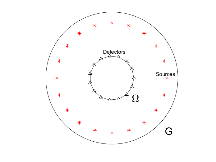
Figure 1: A schematic diagram of domains $G,\Omega,$ sources and detectors.

However, when constructing the required orthonormal basis $\left\{\psi_{n}\left(s\right)\right\}_{n=0}^{\infty},$ we still have used functions $\left\{s^{n}e^{s}\right\}_{n=0}^{\infty},$ i.e. we did not impose the periodicity condition on this basis. The source function $f\left(x\right)$ in our case is the bump function below:

$$f\left(x-x^{\left(s\right)}\right)=\left\{\begin{array}[]{l}\frac{1}{\varepsilon}\exp\left(-\frac{1}{1-\left|x-x_{s}\right|^{2}/\varepsilon}\right),\text{ }if\text{ }\left(x-x_{s}\right)^{2}<\varepsilon,\\ 0,\text{ otherwise.}\end{array}\right.$$

We have chosen $\varepsilon=0.01$.

We use 32 sources and 32 detectors. In examples 1-5 both sources and detectors are uniformly distributed over the whole circle $\{x_{1}^{2}+x_{2}^{2}=4\}$ and the whole circle $S_{1}=\{x_{1}^{2}+x_{2}^{2}=1\}$ respectively. However, this changes in Example 6 (see below).

To solve the forward problem (4), we have used the standard FEM. However, to minimize functional (57), we have written the differential operators in it via finite differences. Thus, we have not committed “inverse crime”. To use the finite differences, we have discretized the domain $\Omega_{\mu}$ in polar coordinates using the uniform finite difference mesh. Next, we have used the gradient descent method to minimize functional (57) with respect to the values of the vector function $W\left(r,\varphi\right)$ at grid points. As the basis $\psi_{k}$ is not periodic over $[0,2\pi]$, we treat numerically $s=0$ and $s=2\pi$ as two different discrete points.

As to the choice of the parameter $\lambda,$even though the above theory works only for sufficiently large values of $\lambda$, we have established in our computational experiments that the choice

(99) $$\lambda=1$$

is sufficient for all six tests we have performed. We have also tested three different values of the number $N$ terms in the series (17):

(100) $$N=4,6,8.$$

Our computational results indicate that $N=8$ is the best choice out of these three.

Remark 6.1. The choice (99) of the parameter $\lambda$ corresponds well with the observations of previous publications on numerical studies of the convexification method, both for coefficient inverse problems with the single location of the source [26, 29, 30] and for ill-posed problems for quasilinear parabolic equations [5, 28]. This observation is that not large values of $\lambda$ can be chosen in computations.

6.2 A multi-level method of the minimization of functional (57)

We have found in our computational experiments that the gradient descent method for our weighted Tikhonov-like functional (57) converges rapidly on a coarse mesh. This provides us with a rough image. Hence, we have implemented a multi-level method [33]. Let $M_{h_{1}}\subset M_{h_{2}}...\subset M_{h_{K}}$ be nested finite difference meshes, i.e. $M_{h_{k}}$ is a refinement of $M_{h_{k-1}}$ for $k\leq K$. Let $P_{h_{k}}$ be the corresponding finite difference functional space. One the first level $M_{h_{1}}$, we solve the discrete optimization problem. In other words, let $V_{h_{1},\min}$ be the minimizer of the following functional which is found via the gradient descent method

(101) $$J_{\lambda}^{\left(h_{1}\right)}\left(W_{h_{1}}\right)=e^{-2\lambda\left(\mu+\eta\right)}\mathop{\displaystyle\int}\limits_{\Omega_{\mu}}\left[\Delta W_{h_{1}}+\Delta P-F\left(\nabla W_{h_{1}}+\nabla P\right)\right]^{2}e^{2\lambda r}dx,$$

where the integral is understood in the discrete sense. Then we interpolate the minimizer $W_{h_{1},\min,\lambda}$ on the finer mesh $M_{h_{2}}$ and take the resulting vector function $W_{h_{2},\text{int}}$ as the starting point of the gradient descent method of the optimization of the direct analog of functional (101) in which $h_{1}$ is replaced with $h_{2}$ and $W_{h_{1}}$ is replaced with $W_{h_{2}}.$This process was repeated until we got the minimizer $W_{h_{K},\min}$ on the $K_{th}$ level on the mesh $M_{h_{K}}$.

Since $(r,\varphi)\in(0,1)\times(0,2\pi)$, then our first level $M_{h_{1}}$ is set to be the uniform mesh with the mesh size in the $r$ direction to be $1/4$ and the mesh size in the $\varphi$ direction to be $2\pi/8$. For each mesh refinement, we will refine the mesh in both $r$ direction and $\varphi$ direction in a way that we set the mesh size of the refined mesh in both direction to be 1/2 of the previous mesh sizes. On each level $M_{h_{k}}$, as soon as we see that $\|\nabla J_{\lambda}^{(h_{k})}(W_{h_{k}})\|<2\times 10^{-2}$, we refine the mesh and compute the solution on the next level $M_{h_{k+1}}$. In the end, we compute $a_{0}(x)$ using the relation (26) with $s=0$.

Our starting point $W^{\left(0\right)}\left(r,\varphi\right)$ for the vector function $W\left(r,\varphi\right)$ for the gradient descent method on the coarse mesh $M_{h_{1}}$ is set to be the background solution $W^{\left(0\right)}(r,\varphi,1)$ which corresponds to the solution of the problem (4) with $\sigma\left(x\right)\equiv 1$. Hence, our starting point is not located in a small neighborhood of the exact solution.

6.3 Numerical testing

In the tests of this section, we demonstrate the efficiency of our numerical method for imaging of small inclusions as well as for imaging of a smoothly varying function $\sigma\left(x\right),$ i.e. a “stretched” inclusion with a wide range of change of the conductivity inside of it. In particular, we test the case of a rather high contrast 5:1 of the inclusion. In all tests the background value of the conductivity is $\sigma_{bkgr}=1.$ In addition, we test the influence of the number $N$ in (100). We also test the effects of both: the data given only on a part of the boundary and the source running only along a part of the circle $\left\{r=2\right\}.$ In Tests 1-6 we have stopped on the 3rd mesh refinement for all three values of $N$ listed in (100) (except for test 4 where $N=8$). The reason of stopping on the 3rd mesh refinement is that images were changing very insignificantly when on the 3rd mesh refinement, as compared with the second.

All necessary derivatives of the data were calculated using finite differences, just as in previous above cited publications of the first author with coauthors about the convexification [26, 30] with numerical results in them, including the one with noisy experimental data [29]. Just as in those works, we have not observed instabilities due to the differentiation, most likely because the step sizes of finite differences were not too small.

Test 1. First, we test the reconstruction by our method of a single inclusion depicted on Figure 2 a). $\sigma=2$ inside of this inclusion and $\sigma=1$ outside. Hence, the inclusion/background contrast is 2:1. The best result is achieved at $N=8$, see Figures 2.

Test 2. We test now the performance of our method for imaging of two inclusions depicted on Figure 3 a). $\sigma=2$ inside of each inclusion and $\sigma=1$ outside of these inclusions. See Figures 3 for results.

Test 3: In this example, we test the reconstruction method for a single inclusion with a rather high inclusion/background contrast 5:1. The results are shown on Figure 4.

Test 4. We now test our method for the case when the function $\sigma\left(x\right)$ is smoothly varying within an abnormality and with a wide range of variations between 0.4 and 1.6. The results are shown in Figure 5. Again $N=8$ is the best value out of three listed in (100). Thus, our method can accurately image not only “sharp” inclusions as in Tests 1-3, but smoothly varying functions as well.

Test 5. In this example we test the stability of the algorithm with respect to the random noise in the data. We test the most challenging case among ones above: the case of the function $\sigma\left(x\right)$ of Test 4. We set $N=8$. The noise is added for $x\in S_{1}$ and for the source $s$ as in (98), $s\in[0,2\pi]$:

$$g_{0,\text{noise}}(x,s)=g_{0}(x,s)(1+\epsilon\xi_{s})\text{ and }g_{1,\text{noise}}(x,s)=g_{1}(x,s)(1+\epsilon\xi_{s}),$$

where $\varepsilon$ is the noise level and $\xi_{s}$ is the independent random variable depending only on the source position $s$ and uniformly distributed on $[-1,1]$. The computational results are displayed on Figure 6 for the levels of noise of 1% and 10%.

This example indicates that our method is quite stable with respect to the noise in the measured data.

Test 6. In all above tests 1-5 we have used the Dirichlet and Neumann data on the entire boundary $S_{1}$ of our disk $\Omega.$ Also, the source was running along the entire circle $C^{\left(s\right)}$ as in (98). In this test, however, we study the case of incomplete data. First, we work with the case when the source runs over the entire circle (98) while the data $g_{0}\left(x,s\right)$ and $g_{0}\left(x,s\right)$ are measured only on a part of the circle $S_{1}.$ Next, we study the case when the source runs only along a part of the circle $C^{\left(s\right)}$ in (98) while the data are measured on the entire circle $S_{1}.$ We again use $N=8$ and the same function $\sigma\left(x\right)$ as in Test 4.

Figures 7 display results of Test 6. Comparing with the correct image of Figure 5, one can observe that, using 50% of the measured boundary data, one looses about 50% of the internal information. On the other hand, using 50% of the positions of the source, one can still recover the internal conductivity with a rather good accuracy. Hence, it seems to be more important to measure at the entire boundary than to use the entire circle $C^{\left(s\right)}$ for the positions of the source.

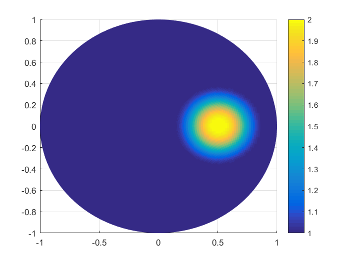
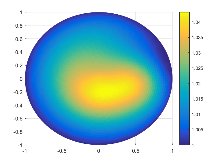
(a) True $\sigma$	(b) $N=4$
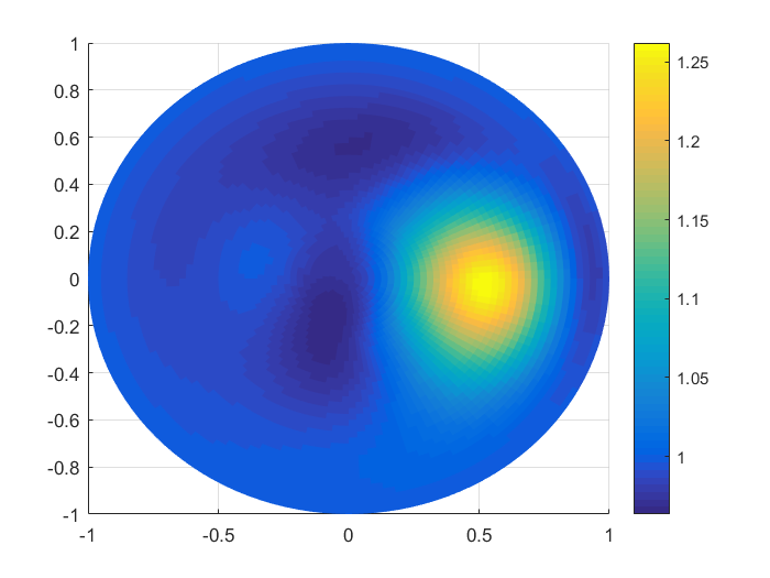
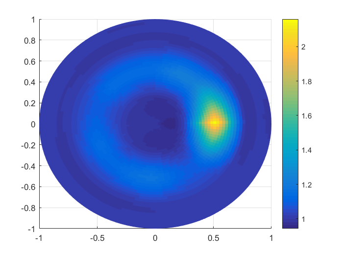
(c) $N=6$	(d) $N=8$

Figure 2: Results of Test 1. Imaging of one inclusion with $\sigma=2$ in it and $\sigma=1$ outside. Hence, the inclusion/background contrast is 2:1. We have stopped at the 3rd mesh refinement for all three values of $N$ listed in (100). a) Correct image. b) Computed image for $N=4$. c) Computed image for $N=6$. d) Computed image for $N=8$. Both the correct contrast and correct location are achieved at $N=8$.

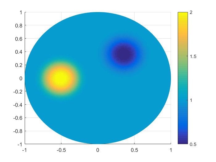
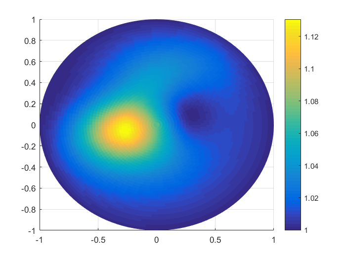
(a) True $\sigma$	(b) $N=4$
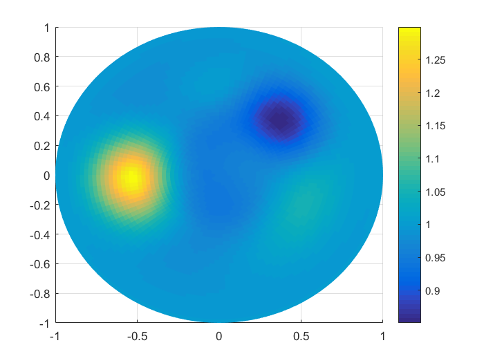
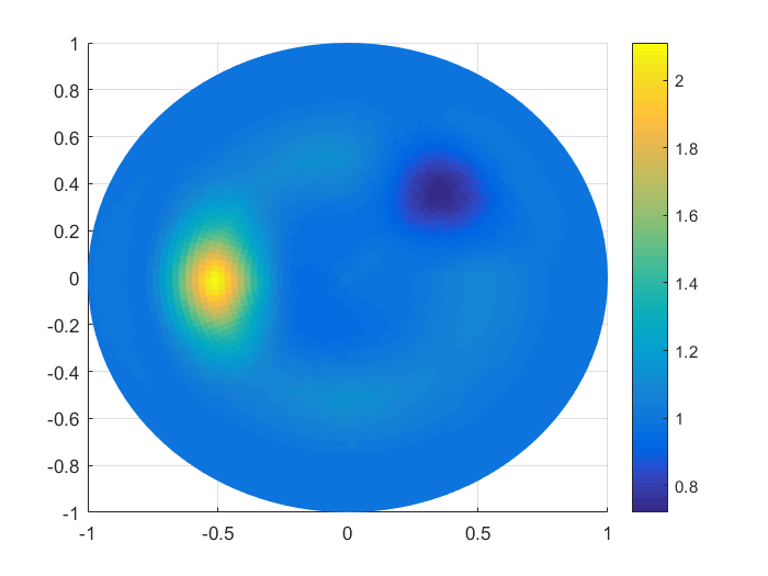
(c) $N=6$	(d) $N=8$

Figure 3: Results of Test 2. Imaging of two inclusions. Here, $\sigma=2$ in the left inclusion, $\sigma=0.5$ in the right inclusion and $\sigma=1$ otherwise. Hence, the inclusion/background contrast is 2:1 in the left inclusion and is 0.5:1 in the right inclusion. This means that the electric conductivity of the left inclusion is higher than the one of the background and it is lower of the right inclusion. We have stopped on the 3rd mesh refinement for all three values of $N$ listed in (100). a) Correct image. b) Computed image for $N=4$. c) Computed image for $N=6$. d) Computed image for $N=8$, which is the best one out of three.

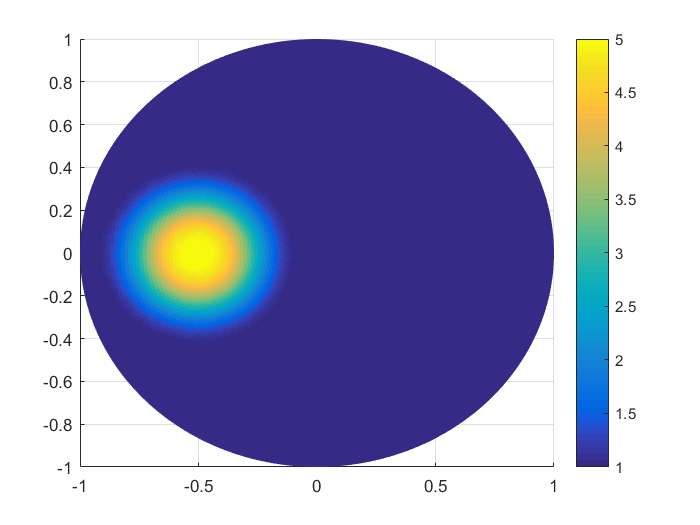
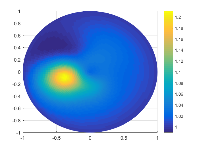
(a) True $\sigma$	(b) $N=4$
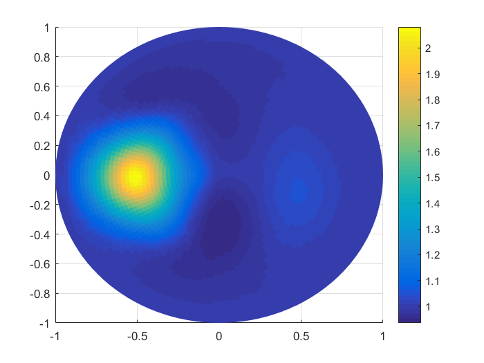
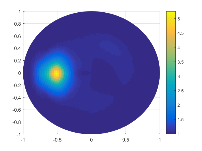
(c) $N=6$	(d) $N=8$

Figure 4: Results of Test 4. Imaging of a single inclusion with a high inclusion/background contrast 5:1. Here, $\sigma=5$ inside the inclusion and $\sigma=1$ outside. a) Correct image. b) Computed image for $N=4$. c) Computed image for $N=6$. d) Computed image for $N=8$, the best one out of three.

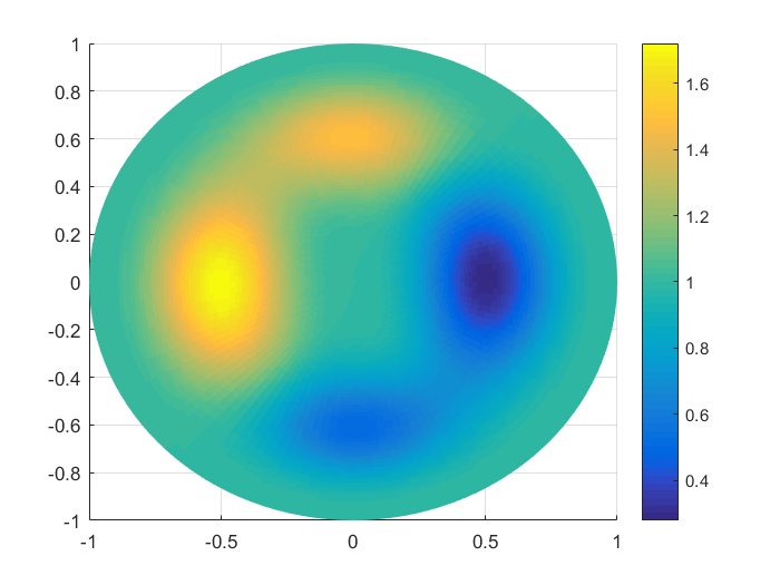
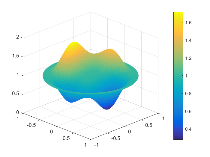
(a) True $\sigma$	(b) 3D view of true $\sigma$
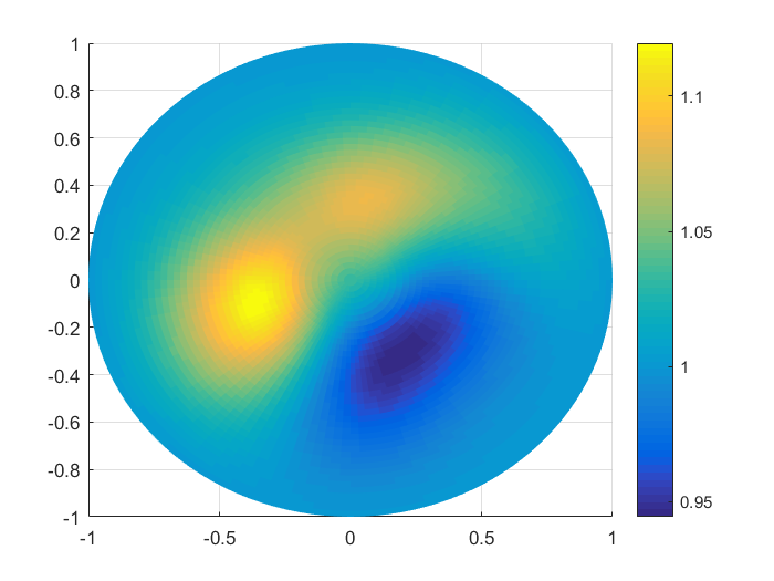
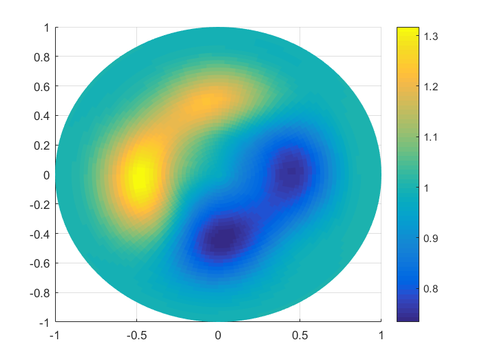
(c) $N=4$	(d) $N=6$
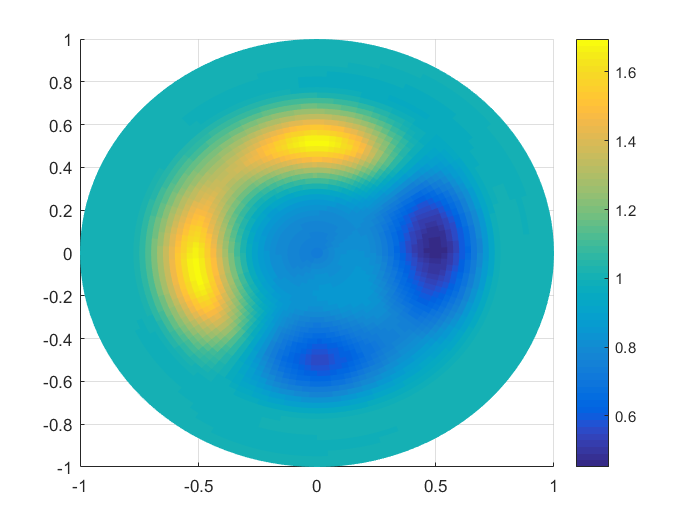
(e) $N=8$	(f) 3D view of the result $N=8$

Figure 5: Results of Test 4. We now test imaging of a smoothly varying conductivity rather than of inclusions above. The values of $\sigma\left(x\right)$ inside of the inhomogenuity vary in a wide range $\sigma_{\min}\approx 0.3$ and $\sigma_{\max}\approx 1.7.$ And $\sigma=1$ in the homogeneous part of this disk. Here, we have stopped on the 3rd mesh refinement. a) Correct 2D image. b) 3D presentation of a). c) Computed image for $N=4$. d) Computed image for $N=6$. e) Computed 2D image for $N=8$. f) 3D presentation of e). Thus, we can accurately image not only “sharp” inclusions but smoothly varying functions as well.

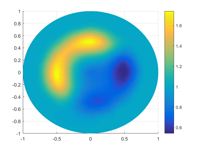
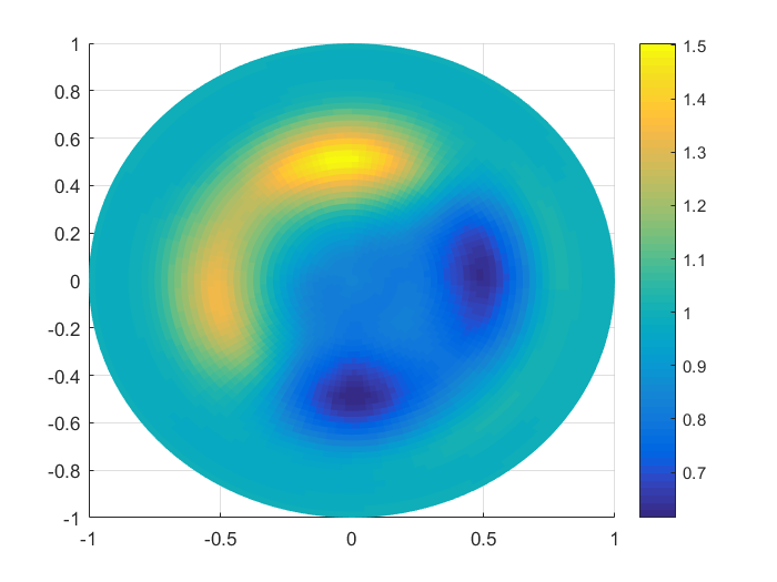
(a) Noise level $1\%$	(b) Noise level $10\%$.

Figure 6: Results of Test 5. In this test we have introduced random noise in the data of test 4. Here, $N=8$. a) Computed image with 1% noise. b) Computed image with 10% noise.

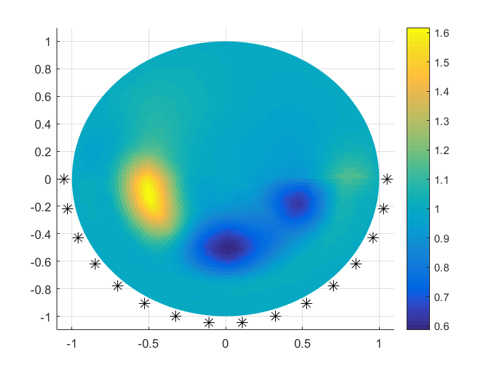
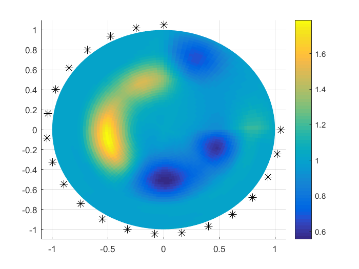
(a) $50\%$ of the boundary data	(b) $75\%$ of the boundary data
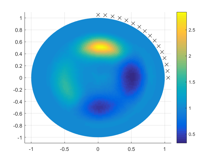
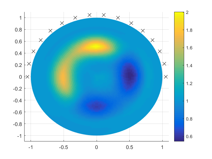
(c) $25\%$ of the position of the source	(d) $50\%$ of the position of the source

Figure 7: Results of Test 6. While the structure to be imaged is the same as the one of Figure 4a), a lesser amount of data is used here. In a) and b) we use incomplete boundary data on the circle $S_{1}=\left\{r=1\right\}$, while the source is still running as in (98): $s\in\left(0,2\pi\right),$ i.e. over the entire circle $C^{\left(s\right)}=\left\{r=4\right\}.$ On the other hand, in c) and d) the boundary data are measured at the entire circle $S_{1}=\left\{r=1\right\},$ while the source is running over only a part of the circle $C^{\left(s\right)}=\left\{r=4\right\}.$ In a) and b) $\ast$ indicates the part of the circle $S_{1}=\left\{r=1\right\}$ where the data are measured. In c) and d) $\times$ indicates the part of the circle $\left\{r=4\right\}$ where the source runs. The part with $\times$ is depicted on $\left\{r=1\right\}$ rather than on $\left\{r=4\right\}$ only for the convenience of the presentation.

7 Concluding remarks

Using a new concept, which was proposed in [31], we have developed here the convexification numerical method for the inverse problem of Electrical Impedance Tomography. While in all past publications on the convexification [8, 22, 27, 26, 29, 30] only a single location of the source was used for either time dependent or frequency dependent data, in the current paper the Dirichlet and Neumann data are generated by a point source running along an interval of a straight line and these data are independent on neither time nor frequency. We have proved theorems, assuring the global convergence of our method. The key analytical tool here is the tool of Carleman estimates. In particular, we have proven two new Carleman estimates.

We have conducted extensive numerical testing of our method. Our computational results demonstrate that this technique can accurately image both sharp inclusions and smoothly varying abnormalities. In addition, our method is quite stable with respect to the noise in the data (Test 5). We have also studied numerically the performance of our method for the case when either boundary data are measured only on a part of the boundary or the source is running only on a part of the circle surrounding our domain of interest.

References

- [1] M. Alsaker and J. L. Mueller. A d-bar algorithm with a priori information for 2-dimensional electrical impedance tomography, SIAM Journal on Imaging Sciences, 9 (2016), pp. 1619-1654.
- [2] H. Ammari, G. S. Alberti, B. Jin, J. K. Seo, and W. Zhang. The linearized inverse problem in multifrequency electrical impedance tomography, SIAM Journal on Imaging Sciences, 9 (2016), pp. 1525-1551.
- [3] H. Ammari and H. Kang. Reconstruction of small inhomogeneities from boundary measurements, Springer-Verlag, Berlin, 2004.
- [4] H. Ammari, L. Qiu, F. Santosa, and W. Zhang. Determining anisotropic conductivity using diffusion tensor imaging data in magneto-acoustic tomography with magnetic induction, Inverse Problems, 33 (2017), pp. 125006.
- [5] A. B. Bakushinskii, M. V. Klibanov and N. A. Koshev, Carleman weight functions for a globally convergent numerical method for ill-posed Cauchy problems for some quasilinear PDEs, Nonlinear Analysis: Real World Applications, 34 (2017), pp. 201–224.
- [6] L. Baudouin, M. de Buhan and S. Ervedoza, Convergent algorithm based on Carleman estimates for the recovert of a potential in the wave equation, SIAM J. on Numerical Analysis, 55 (2017), pp. 1578-1613.
- [7] L. Beilina and M. V. Klibanov, Approximate Global Convergence and Adaptivity for Coefficient Inverse Problems, Springer, New York, 2012.
- [8] L. Beilina and M. V. Klibanov, Globally strongly convex cost functional for a coefficient inverse problem, Nonlinear Analysis: Real World Applications, 22 (2015), pp. 272–288.
- [9] M. Bellassoued and M. Yamamoto, Carleman Estimates and Applications to Inverse Problems for Hyperbolic Systems, Springer Japan KK, 2017.
- [10] A. Bukhgeim and M. Klibanov, Uniqueness in the large of a class of multidimensional inverse problems, Soviet Math. Doklady, 17 (1981), pp. 244–247.
- [11] L. Borcea. Electrical impedance tomography, Inverse Problems, 18 (2002), pp. R99-R136.
- [12] A. P. Calderon. On an inverse boundary value problem, Seminar on Numerical Analysis and its Applications to Continuum Physics (Rio de Janeiro, 1980), Soc. Brasil. Mat., Rio de Janeiro, pp. 65–73.
- [13] M. Dodd and J. Mueller. A real-time d-bar algorithm for 2-d electrical impedance tomography data, Inverse Probl Imaging (Springfield). 8 (2014), pp. 1013-1031.
- [14] D. Gilbarg and N.S. Trudinger, Elliptic Partial Differential Equations of Second Order, Springer, New York, 1984.
- [15] S. J. Hamilton, M. Lassas, and S. Siltanen. A direct reconstruction method for anisotropic electrical impedance tomography, Inverse Problems, 30 (2014), pp. 075007.
- [16] S. J. Hamilton, J. M. Reyes, S. Siltanen, and X. Zhang. A hybrid segmentation and d-bar method for electrical impedance tomography, SIAM Journal on Imaging Sciences, 9 (2016), pp. 770–793.
- [17] B. Harrah and M.N. Minh, Enhancing residual-based techniques with shape reconstruction features in Electrical Impedance Tomography, Inverse Problems, 32 (2016), pp. 125002.
- [18] D. Holder. Electrical Impedance Tomography: Methods, History and Applications, Institute of Physics, Bristol, 2005.
- [19] N. Hyvnen , L. Pivrinta and J. P. Tamminen Enhancing D-bar reconstructions for electrical impedance tomography with conformal maps. Enhancing D-bar reconstructions for electrical impedance tomography with conformal maps, Inverse Problems and Imaging, 12 (2018), pp. 373-400.
- [20] B. Jin, T. Khan, and P. Maass. A reconstruction algorithm for electrical impedance tomography based on sparsity regularization, International Journal for Numerical Methods in Engineering, 89 (2012), pp. 337–353.
- [21] B. Jin, Y. Xu, and J. Zou. A convergent adaptive finite element method for electrical impedance tomography, IMA Journal of Numerical Analysis, 37 (2017), pp. 1520–1550.
- [22] M. V. Klibanov, Global Convexity in a Three-Dimensional Inverse Acoustic Problem, SIAM Journal on Mathematical Analysis, 28 (1997), pp. 1371–1388.
- [23] M. V. Klibanov, Carleman estimates for global uniqueness, stability and numerical methods for coefficient inverse problems, Journal of Inverse and Ill-Posed Problems, 21 (2013), pp. 477–560.
- [24] M. V. Klibanov, Carleman estimates for the regularization of ill-posed Cauchy problems, Applied Numerical Mathematics, 94 (2015), pp. 46–74.
- [25] M. V. Klibanov, Carleman weight functions for solving ill-posed Cauchy problems for quasilinear PDEs, Inverse Problems, 31 (2015), pp. 125007.
- [26] M. V. Klibanov and N. T. Thành, Recovering Dielectric Constants of Explosives via a Globally Strictly Convex Cost Functional, SIAM Journal on Applied Mathematics, 75 (2015), pp. 518–537.
- [27] M. V. Klibanov and V. G. Kamburg, Globally strictly convex cost functional for an inverse parabolic problem, Mathematical Methods in the Applied Sciences, 39 (2016), pp. 930–940.
- [28] M. V. Klibanov, N.A. Koshev, J. Li and A.G. Yagola, Numerical solution of an ill-posed Cauchy problem for a quasilinear parabolic equation using a Carleman weight function, J. Inverse and Ill-Posed Problems, 24 (2016), pp. 761-776.
- [29] M. V. Klibanov, A. E. Kolesov, L. Nguyen and A. Sullivan, Globally strictly convex cost functional for a 1-D inverse medium scattering problem with experimental data, SIAM J. Applied Mathematics, 77 (2017), pp. 1733-1755.
- [30] M. V. Klibanov and A. E. Kolesov, Convexification of a 3-D coefficient inverse scattering problem, accepted in Computers and Mathematics with Applications, 2018, also see arxiv: 1801.04404.
- [31] M.V. Klibanov, Convexification of restricted Dirichlet-to-Neumann map, J. Inverse and Ill-Posed Problems, 25 (2017), pp. 669-685.
- [32] O. Kwon, J.-K. Seo, and J.-R. Yoon. A real-time algorithm for the location search of discontinuous conductivities with one measurement, Comm. Pure Appl. Math., 55 (2002), pp. 1–29.
- [33] J. Li and J. Zou. A multilevel model correction method for parameter identification, Inverse Problems, 23 (2007), pp. 1759.
- [34] M.M. Lavrentiev, V.G. Romanov and S.P. Shishatskii, Ill-Posed Problems of Mathematical Physics and Analysis, AMS, Providence, R.I., 1986.
- [35] G. Matthias, J. Bangti, and L. Xiliang. An analysis of finite element approximation in electrical impedance tomography, Inverse Problems, 30 (2014), pp. 045013.
- [36] A. Nachman, Global uniqueness for a two-dimensional inverse boundary value problem, Annals of Mathematics, 143 (1996), pp. 71-96.
- [37] J. A. Scales, M. L. Smith, and T. L. Fischer, Global optimization methods for multimodal inverse problems, Journal of Computational Physics, 103 (1992), pp. 258–268.
- [38] J. K. Seo, J. Lee, S. W. Kim, H. Zribi, and E. J. Woo. Frequency-difference electrical impedance tomography (fdEIT): algorithm development and feasibility study, Phys. Meas., 29 (2008), pp. 929–944.
- [39] J.-K. Seo and E.-J. Woo. Magnetic resonance electrical impedance tomography (MREIT). SIAM Rev., 53 (2011), pp. 40–68.
- [40] J. Sylvester and G. Uhlmann, Global uniqueness theorem for an inverse boundary problem, Annals of Mathematics, 39 (1987), pp. 91-112.
- [41] A.N. Tikhonov, A.V. Goncharsky, V.V. Stepanov and A.G. Yagola, Numerical Methods for the Solution of Ill-Posed Problems, Kluwer, London, 1995.
- [42] T. Widlak and O. Scherzer. Hybrid tomography for conductivity imaging, Inverse Problems, 28(2012), pp. 084008.