Lindblad-Floquet description of finite-time quantum heat engines

Abstract

The operation of autonomous finite-time quantum heat engines rely on the existence of a stable limit cycle in which the dynamics becomes periodic. The two main questions that naturally arise are therefore whether such a limit cycle will eventually be reached and, once it has, what is the state of the system within the limit cycle. In this paper we show that the application of Floquet’s theory to Lindblad dynamics offers clear answers to both questions. By moving to a generalized rotating frame, we show that it is possible to identify a single object, the Floquet Liouvillian, which encompasses all operating properties of the engine. First, its spectrum dictates the convergence to a limit cycle. And second, the state within the limit cycle is precisely its zero eigenstate, therefore reducing the problem to that of determining the steady-state of a time-independent master equation. To illustrate the usefulness of this theory, we apply it to a harmonic oscillator subject to a time-periodic work protocol and time-periodic dissipation, an open-system generalization of the Ermakov-Lewis theory. The use of this theory to implement a finite-time Carnot engine subject to continuous frequency modulations is also discussed.

I Introduction

The last decades have witnessed remarkable progress in the experimental manipulation of a variety of quantum platforms, enabling for the first time the coherent control over genuinely quantum mechanical resources. This progress has in turn motivated substantial research in addressing which types of applications may be drawn up using such platforms. One promising such avenue concerns the use of quantum effects in the operation of heat engines and refrigerators Alicki1979; Rezek2006; Kosloff2014; Abah2012; Alicki2015. This would allow, for instance, to extend the efficiency above classical bounds using non-equilibrium reservoirs Abah2014; Klaers2017a; Ronagel2014; Correa2014; Jaramillo2016; Samuelsson2017, operate adiabatic cycles at finite times using shortcuts to adiabaticity DelCampo2014; Abah2016; Abah2017, implement informationally driven engines Camati2016; Elouard2017; Cottet2017; Masuyama2017; Manzano2017b and even substitute work and heat by quantum resources, such as entanglement Micadei2017 and coherence Manzano2017.

Despite the surge in interest, several scenarios still remain unexplored, with most studies so far having focused on either continually operated engines, such as absorption refrigerators Kosloff2014; Kilgour2018; Latune2018; Schilling; Holubec2018; Hofer2018 or stroke-based engines, with a particular focus on the Otto cycle Alicki1979; Rezek2006; Kosloff2014; Abah2012; Alicki2015; Abah2014; Klaers2017a; Ronagel2014; Correa2014; Jaramillo2016; Samuelsson2017; DelCampo2014; Abah2016; Abah2017; Insinga2018; Insinga2016; Feldmann1996; Feldmann2004; Rezek2006a; Watanabe2017; Kieu2004; Song2016; Altintas2015. Carnot or Stirling cycles have also been studied, but to a lesser extent He2002; Quan2009; Gardas2015; Brandner2016. The same is true for continually operated work protocols Alicki2006; Alicki2012; Kosloff2013; Szczygielski2013.

The main reason behind the focus on the Otto cycle is due to its convenient separation of the work and heat strokes, which facilitates the theoretical modeling since it allows one to use unitary dynamics for the former and time-independent dissipative dynamics for the later. Moreover, it is usually assumed that the heat strokes act for a sufficiently long time so as to allow for a full thermalization. Studies dealing with finite-time operations over all strokes remain scarce. In this case a subtle question arises concerning the convergence or not to a limit-cycle, in which the operation of the engine becomes periodic. As shown in Insinga2018; Insinga2016; Feldmann1996; Feldmann2004; Watanabe2017, depending on the work protocol and its corresponding injection of energy, unusually large values of dissipation may be necessary in order to obtain a stable cycle. Consequently, these considerations may have an important impact in translating optimization protocols, such as shortcuts to adiabaticity, to the finite-time regime.

In the context of finite-time engines, the problem may therefore be divided in two parts. The first is the convergence towards a limit cycle and the second concerns the behavior of the system within this cycle. A more thorough understanding of these two features is therefore essential for advancing our theoretical understanding of quantum heat engines. However, such advances are hampered by the lack of a consistent theoretical framework to address the properties of the cycle as a whole, instead of each individual stroke.

In this paper we attempt to fulfill this gap by showing how the operation of a heat engine may be neatly formulated in terms of Floquet’s theory applied to Lindblad dynamics. Instead of analyzing each stroke separately, we consider the full cycle as modeled by a time-dependent periodic Liouvillian $\mathcal{L}_{t}$. Then, applying Floquet’s theory and moving to a generalized rotating frame, we show how all relevant aspects of the heat engine are completely dictated by a super-operator $\mathcal{L}_{F}(t)$, which we refer to as Floquet Liouvillian. First, the convergence to a limit cycle is directly associated to the eigenvalues of $\mathcal{L}_{F}(t)$ (which are independent of $t$). Second, the state of the system after the limit-cycle has been reached is precisely the zero-eigenstate of $\mathcal{L}_{F}(t)$, with $t$ as a parameter. This therefore reduces the problem of finding the limit cycle to that of finding the steady-state of a time-independent master equation.

Floquet theory has seen a boom of interest in the last decades, specially due to its potential use in quantum simulation. Important advances in its extension to open quantum systems have also appeared recently Haddadfarshi2015; Wu2015a; Restrepo2016; Hartmann2016b; Dai2016; Alicki2006; Alicki2012. In particular, we call attention to Refs. Alicki2006; Alicki2012 where the authors describe a method to derive quantum master equations for systems subject to a periodically driven Hamiltonian and in contact with a heat bath. Such a framework has direct applications in the context of quantum heat engines (c.f. Szczygielski2013; Kosloff2014). However, it cannot be used to describe stroke-based engines containing unitary (isentropic) branches, such as the Carnot cycle, since it assumes that the system-bath coupling remains on at all times. To do so, one must be able to couple and uncouple the system from the bath periodically. Although there are ways of bypassing this, such as using sufficiently fast drives or implementing protocols which ensure that the heat flow is zero on average Martinez2015a; Martinez2015, in order to describe Carnot and related cycles in all generality, one must eventually make use of some uncoupling mechanism. This is the main advantage behind our approach. We shall take as a starting point an arbitrary master equation, but whose parameters are assumed to vary periodically following some protocol (while ensuring complete positivity at all times). Even though this has the disadvantage of loosing the microscopic interpretation of a system-environment coupling, it has the advantage of being able to deal with arbitrary coupling protocols. Moreover, it also works for engineered reservoirs and phenomenological equations.

To illustrate the usefulness of this theory, we apply it to the exactly soluble model of a harmonic oscillator under the influence of an arbitrary time-periodic work protocol and arbitrary time-periodic and Gaussian-preserving environments. This corresponds to an open-system generalization of the Ermakov-Lewis theory Lewis1967; Lewis1968; Jeremie2010; Scopa2018 describing a harmonic oscillator subject to a frequency modulation. In our theory all parameters may be time-dependent, including the frequency, mass, damping rate, temperature and squeezing (magnitude and angle), provided they all share the common period of the cycle. This therefore allows one to implement any type of single-oscillator engine, including protocols for shortcuts to adiabaticity or the use of (possibly time-dependent) squeezing effects to maximize efficiency. Given the widespread use of harmonic systems as working fluids, we believe that these results should prove valuable in the design and optimization of more efficient engines. As an example, we briefly discuss their application to the study of a finite-time Carnot engine.

II Lindblad-Floquet theory

We consider here an arbitrary quantum heat engine operating periodically with period $\mathcal{T}$. The different strokes of the engine may contain both unitary and dissipative contributions. Instead of describing these effects separately, we combine them into a single master equation for the working fluid’s density matrix $\rho(t)$, subject to a certain time-dependent periodic Liouvillian operator $\mathcal{L}_{t}$ satisfying $\mathcal{L}_{t+\mathcal{T}}=\mathcal{L}_{t}$. For convenience we write the master equation in super-operator space as

$$\frac{\,\mathrm{d}|\rho_{t}\rangle}{\,\mathrm{d}t}=\mathcal{L}_{t}|\rho_{t}\rangle,$$ (1)

where $|\rho_{t}\rangle$ is the density matrix written in vectorized form.

To clarify our notation, let us consider the implementation of an Otto cycle. Let $\Omega(t)$ denote a generic work parameter, $\gamma(t)$ the bath-coupling constant and $T(t)$ the temperature. An Otto cycle would then be described by the following protocol (see Fig. 1(b)): rCl Ω: &   (Ω_1, Ω_2(t), Ω_3, Ω_4(t)),
γ:   (γ_1,0,γ_3,0),
T:   (T_H, -, T_C, -). The first and third strokes are the thermalization (isochoric) heat strokes for which the work parameter is fixed and the system is allowed to partially relax in contact with heat baths at temperatures $T_{H}$ and $T_{C}$. The second and fourth strokes, on the other hand, are the unitary (isentropic) work strokes for which the system is detached from the bath ($\gamma=0$). Each stroke may have different durations but we denote by $\mathcal{T}$ the total period of the cycle. It is clear from this example that any type of cycle may be constructed by appropriately choosing the parameters in the master equation. For instance, the protocol for constructing a Carnot cycle is illustrated in Fig. 1(c).

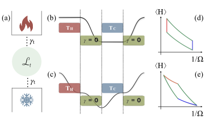
Figure 1: Modeling of quantum heat engines using Lindblad-Floquet theory. (a) A thermodynamic cycle, for instance with a harmonic oscillator as working fluid, may be described by means of a time-periodic Liouvillian $\mathcal{L}_{t}$ which encompasses the evolution of the work parameter $\Omega(t)$, the different bath temperatures $T_{H}$ and $T_{C}$, and the on-off protocol for the bath couplings, modeled by $\gamma_{t}$. (b,c) Diagrams for the Otto and Carnot cycles respectively. The green regions correspond to the unitary expansion and compression strokes, whereas the red and blue regions denote the interactions with the two reservoirs. The black curves illustrate typical work protocols $\Omega(t)$ for the two cycles. In the Otto cycle $\Omega$ is constant in the red and blue regions, whereas in the Carnot cycle the hot isothermal is an expansion and the cold isothermal a compression. (d,e) The corresponding quasi-static cycles in a $\langle H\rangle$ vs. $1/\Omega$ diagram.

We now cast the master Eq. (1) within the framework of Floquet’s theory. We begin by moving to a generalized rotating frame by defining a new state $|\tilde{\rho}_{t}\rangle=W(t)|\rho_{t}\rangle$, where $W(t)$ is a time-periodic super-operator. In this rotating frame $|\tilde{\rho}_{t}\rangle$ will satisfy an equation analogous to (1), but subject to the effective Liouvillian

$$\tilde{\mathcal{L}}=W(t)\mathcal{L}_{t}W^{-1}(t)+\frac{\,\mathrm{d}W(t)}{\,\mathrm{d}t}W^{-1}(t).$$ (2)

If we can now choose $W(t)$ such that $\tilde{\mathcal{L}}$ is time-independent, then the evolution in this rotating frame, between times $t_{0}$ and $t$, will be given simply by $|\tilde{\rho}_{t}\rangle=e^{(t-t_{0})\tilde{\mathcal{L}}}|\tilde{\rho}_{t_{0}}\rangle$. Moving back to the original frame then allows us to write the evolution of $|\rho_{t}\rangle$ as

$$|\rho_{t}\rangle=K(t,t_{0})e^{(t-t_{0})\mathcal{L}_{F}(t_{0})}|\rho_{t_{0}}\rangle,$$ (3)

where we have defined the Floquet Liouvillian

$$\mathcal{L}_{F}(t_{0})=W^{-1}(t_{0})\tilde{\mathcal{L}}W(t_{0}),$$ (4)

and the micromotion super-operator

$$K(t,t_{0})=W^{-1}(t)W(t_{0}).$$ (5)

Since $W(t)$ is periodic, it follows that $\mathcal{L}_{F}(t_{0}+\mathcal{T})=\mathcal{L}_{F}(t_{0})$. The same is true for both arguments of $K(t,t_{0})$.

From Eq. (5) one also has that $K(t_{0},t_{0})=1$. Hence, the stroboscopic evolution of the system will be governed solely by the Floquet Liouvillian

$$|\rho_{t_{0}+n\mathcal{T}}\rangle=e^{n\mathcal{T}\mathcal{L}_{F}(t_{0})}|\rho_{t_{0}}\rangle.$$ (6)

This leads us to our first main result: A sufficient condition for the system to converge to a limit cycle is that all eigenvalues of $\mathcal{L}_{F}(t_{0})$ have a non-positive real part. Instead of looking at $\mathcal{L}_{F}(t_{0})$, one may also look directly at $\tilde{\mathcal{L}}$ since the two are connected by a similarity transformation [Eq. (4)]. As will be illustrated below, this will in general be much simpler and also serves to show that the spectrum of $\mathcal{L}_{F}(t_{0})$ is independent of $t_{0}$.

Next let $|\rho_{F}(t_{0})\rangle$ denote the steady-state of $\mathcal{L}_{F}(t_{0})$; that is, $\mathcal{L}_{F}(t_{0})|\rho_{F}(t_{0})\rangle=0$. For simplicity, we will henceforth assume that this steady-state is unique. Then, after a sufficiently long time, the engine will eventually converge to a limit cycle for which the density matrix becomes periodic, being given by:

$$|\rho_{t}\rangle=K(t,t_{0})|\rho_{F}(t_{0})\rangle.$$ (7)

However, since the micromotion is periodic, we may now set $t_{0}=t$, which then finally gives

$$|\rho_{t}\rangle=|\rho_{F}(t)\rangle.$$ (8)

This is our second main result: within the limit-cycle the state of the system will be simply the zero eigenstate of $\mathcal{L}_{F}(t)$, provided this eigenstate is unique. This result is a consequence of the convergence towards a steady-state. It is therefore a feature unique of open systems and allows for a remarkable simplification in the description of the problem.

It is also useful to compare these results with the method developed in Refs. Alicki2006; Alicki2012, which consists in generalizing the microscopic derivations to include a periodic drive in the system Hamiltonian. Our approach can therefore be viewed as complementary. We assume no information about the environment or the processes which led to the master equation. Instead, we take the Liouvillian as given and then cast it in terms of Floquet’s theory to extract its main properties. This has the advantage of allowing for the coupling constant and the bath temperature to be turned on and off at will. One should note, however, that even if the bath parameters are constant, both models may not necessarily give the same result. The reason is that in the method of Refs. Alicki2006; Alicki2012 one takes into account the effects that the driving on the system have on the exchange of excitations between system and bath. However, it is expected that these effects will become important only if the time-scales of the drive become comparable with the bath correlation times. If that is not the case, then from physical grounds one expects that the master equation will be such that it instantaneously thermalize the system at each instant of time.

We also would like to call attention to some known difficulties of dealing with Floquet Liouvillians. Even though the computation of the stroboscopic map (6) is always well defined, the calculation of the Floquet Liouvillian $\mathcal{L}_{F}$ may be problematic, leading to generators that do not preserve complete positivity. A numerically exact illustration of this was given recently in Fig. 4 of Ref. Hartmann2016b. This can turn out to be a serious issue when one is interested in finding $\mathcal{L}_{F}$ by means of high-frequency Magnus expansions, which is often the case since the problem is usually analytically intractable. In this sense, another important development to call attention to is Ref. Haddadfarshi2015, where the authors have developed a method to build high-frequency Magnus expansions that preserve complete positivity at all orders. Interestingly, the seeming inconsistency between this and the results in Ref. Hartmann2016b, seem to point to a limited radius of convergence of the Magnus expansion. Here we shall avoid this issue by looking at an exactly soluble model for which the dynamics is always completely positive.

III Application to a harmonic oscillator

We now consider the exactly soluble model of a bosonic mode, described by an annihilation operator $a$, subject to an arbitrary time-dependent and Gaussian-preserving open system dynamics. Here we provide only the main ideas and results, leaving some of the technical details to the appendices. The Hamiltonian of the system is chosen to be

$$H_{t}=\omega_{t}(a^{\dagger}a+\nicefrac{{1}}{{2}})+\frac{\lambda_{t}}{2}aa+\frac{\lambda_{t}^{*}}{2}a^{\dagger}a^{\dagger}.$$ (9)

where $\omega_{t}$ and $\lambda_{t}$ are arbitrary periodic functions satisfying $\omega_{t}^{2}>|\lambda_{t}|^{2}$. In a mechanical picture, the Hamiltonian (9) describes a situation where both the mass and the spring constant may be time-dependent. The situation where the mass is constant corresponds to $\eta:=\omega_{t}-\lambda_{t}$ being time-independent, in which case the mechanical frequency $\Omega_{t}$ is given by $\Omega_{t}^{2}=\omega_{t}^{2}-\lambda_{t}^{2}$ (see Appendix LABEL:sec:relation).

The Hamiltonian (9) adds to $\mathcal{L}_{t}$ three super-operators: rCl H_0 &= - i [a^†a, ∙],
H_1 = - i [a a, ∙],
H_2 = - i [a^†a^†, ∙]. In addition, we consider the general effects of Gaussian preserving dissipation generated by rCl D_1 = a ∙a^†- 12 {a^†a, ∙}, &   D_2 = a^†∙a - 12 { a a^†, ∙},
D_3 = a^†∙a^†- 12 { a^†a^†, ∙},    D_4 = a ∙a - 12 { a a, ∙}. With these ingredients, we then parametrize our time-dependent Liouvillian as

$$\mathcal{L}_{t}=\mathcal{H}_{t}+\mathcal{D}_{t},$$ (10)

where rCl H_t &= ω_t H_0 + λt2 H_1 + λt*2 H_2,
D_t = γ_t (N_t +1) D_1 + γ_t N_t D_2 - γ_t M_t D_3 - γ_t M_t^* D_4. where $\gamma_{t}$, $N_{t}$ and $M_{t}$ are periodic parameters satisfying $\gamma_{t}>0$ and $N_{t}(N_{t}+1)>|M_{t}|^{2}$. Here $\gamma_{t}$ represents the coupling strength to the bath, whereas $N_{t}$ and $M_{t}$ may represent both thermal and squeezing effects, depending on the choice of basis. For instance, if $\lambda_{t}=0$ then a thermal bath at a temperature $T$ correspond to $M_{t}=0$ and $N_{t}=(e^{\omega_{t}/T}-1)^{-1}$. For the general Hamiltonian (9), on the other hand, the thermal bath is modeled by

$$N_{t}+\nicefrac{{1}}{{2}}=\frac{\omega_{t}}{2\Omega_{t}}\coth\bigg{(}\frac{\Omega_{t}}{2T}\bigg{)},\quad M_{t}=-\frac{\lambda_{t}}{2\Omega_{t}}\coth\bigg{(}\frac{\Omega_{t}}{2T}\bigg{)},$$ (11)

where $\Omega_{t}^{2}=\omega_{t}^{2}-\lambda_{t}^{2}$.

Next we apply the rotating frame transformation (2). The key property making this problem analytically tractable and free of the aforementioned positivity issues is that the 7 super-operators $\{\mathcal{H}_{i},\mathcal{D}_{i}\}$ form a closed algebra PeixotoDeFaria2007 (see also Ryabov2013). In particular, the sets $\{\mathcal{H}_{i}\}$ and $\{\mathcal{D}_{i}\}$, when taken separately, satisfy independent algebras: rCl [H_0, H_1,2] &= ±2 i H_1,2,   [H_1, H_2] = -4 i H_0, and rCl [D_1, D_2] &= -(D_1 + D_2),   [D_3, D_4] = 0,

[D_1, D_3,4] = -D_3,4,   [D_2, D_3,4] = D_3,4, Mixtures of the two sets, on the other hand, only produce elements of the latter: rCLccrl [H_0, D_1,2] &= 0,    [H_0, D_3,4] = ∓2 i D_3,4,
[H_1, D_1,2] = -2 i D_4,    [H_2, D_1,2] = 2 i D_3,
[H_1, D_3] = -2 i (D_1+D_2),    [H_1, D_4] = 0,
[H_2, D_4] = 2 i (D_1+D_2) ,    [H_2, D_3] = 0. This algebraic structure suggests that the operator $W(t)$ in Eq. (2) may be taken as

$$W(t)=V(t)U(t),$$ (12)

where

$$V(t)=e^{g_{1}\mathcal{D}_{1}}e^{g_{2}\mathcal{D}_{2}}e^{g_{3}\mathcal{D}_{3}}e^{g_{4}\mathcal{D}_{4}},$$ (13)

and

$$U(t)=e^{r_{0}\mathcal{H}_{0}}e^{r_{1}\mathcal{H}_{1}}e^{r_{2}\mathcal{H}_{2}}.$$ (14)

Here $r_{i}(t)$ and $g_{i}(t)$ are time-periodic c-number functions which are to be suitably adjusted so as to make $\tilde{\mathcal{L}}$ time-independent. The problem is then solved sequentially. First one applies $U(t)$ and adjusts the $r_{i}(t)$ to make the unitary part time-independent. Then $V(t)$ is applied and the $g_{i}(t)$ are adjusted to deal with the dissipative part. In this section, we shall illustrate the procedure in the simpler case when $\omega=\lambda=0$. That is, when only the dissipative terms are present. The general formulation is presented in Appendices LABEL:sec:gen_uni and LABEL:sec:gen_diss and the main results will be summarized in Sec. LABEL:ssec:app_gen below.

III.1 Purely dissipative case

In the case $\omega=\lambda=0$ the situation simplifies dramatically since only the dissipative part remains in the Liouvillian (10). Consequently, it suffices to choose $U(t)=1$ in Eq. (12). To carry out the rotating frame transformation in Eq. (2) it is necessary to evaluate products such as

$$e^{g_{1}\mathcal{D}_{1}}\mathcal{D}_{2}e^{-g_{1}\mathcal{D}_{1}}=e^{-g_{1}}\mathcal{D}_{2}+(e^{-g_{1}}-1)\mathcal{D}_{1},$$ (15)

which can be found as usual, with the Baker-Campbell-Haussdorff formula. One also requires the identity

$$\frac{\,\mathrm{d}(e^{g_{i}\mathcal{D}_{i}})}{\,\mathrm{d}t}(e^{-g_{i}\mathcal{D}_{i}})=\frac{\,\mathrm{d}g_{i}}{\,\mathrm{d}t}\mathcal{D}_{i}.$$ (16)

Carrying out all computations we then find

$$\tilde{\mathcal{L}}=C_{1}(t)\mathcal{D}_{1}+C_{2}(t)\mathcal{D}_{2}+C_{3}(t)\mathcal{D}_{3}+C_{4}(t)\mathcal{D}_{4},$$ (17)

where rCl C_2(t) &= e^-g_1 [ ˙g