Novel Fourier Quadrature Transforms and Analytic Signal Representations for Nonlinear and Non-stationary Time Series Analysis

Abstract

The Hilbert transform (HT) and associated Gabor analytic signal (GAS) representation are well-known and widely used mathematical formulations for modeling and analysis of signals in various applications. In this study, like the HT, to obtain quadrature component of a signal, we propose the novel discrete Fourier cosine quadrature transforms (FCQTs) and discrete Fourier sine quadrature transforms (FSQTs), designated as Fourier quadrature transforms (FQTs). Using these FQTs, we propose sixteen Fourier-Singh analytic signal (FSAS) representations with following properties: (1) real part of eight FSAS representations is the original signal and imaginary part is the FCQT of the real part, (2) imaginary part of eight FSAS representations is the original signal and real part is the FSQT of the real part, (3) like the GAS, Fourier spectrum of the all FSAS representations has only positive frequencies, however unlike the GAS, the real and imaginary parts of the proposed FSAS representations are not orthogonal to each other. The Fourier decomposition method (FDM) is an adaptive data analysis approach to decompose a signal into a set of small number of Fourier intrinsic band functions which are AM-FM components. This study also proposes a new formulation of the FDM using the discrete cosine transform (DCT) with the GAS and FSAS representations, and demonstrate its efficacy for improved time-frequency-energy representation and analysis of nonlinear and non-stationary time series.

Keywords: Hilbert transform (HT); Gabor analytic signal (GAS) representation; Instantaneous frequency (IF); Fourier Quadrature Transform (FQT); Fourier-Singh analytic signal (FSAS) representations; Zero-phase filtering (ZPF)

1 INTRODUCTION

The Fourier theory is the most important mathematical tool for analysis and modeling physical phenomena and engineering systems. It has been used to obtain solutions in almost all fields of science and engineering problems. It is the fundamentals of a signal analysis, processing, and interpretation of information. There are many variants of the Fourier methods such as continuous time Fourier series (FS) and Fourier transfrom (FT), discrete time Fourier transform (DTFT), discrete time Fourier series (DTFS), discrete Fourier transform (DFT), discrete cosine transform (DCT), and discrete sine transform (DST). All these are orthogonal transforms which can be computed by the fast Fourier transform (FFT) algorithms.

The instantaneous frequency (IF) was introduced by the Carson and Fry [1] in 1937 with application to the frequency modulation (FM), and it was defined as derivative of phase of a complex FM signal. Gabor [2] in 1946 introduced a quadrature method based on the Fourier theory as a practical approach for obtaining the Hilbert Transform (HT) of a signal. Ville [3] in 1948 defined the IF of a real signal by using Gabor complex extension. Shekel [4] in 1953 pointed out ambiguity issue in the IF defined by Ville that there are an infinite number of pairs of instantaneous amplitude (IA) and IF for a complex extension of a given signal. Gabor analytic signal (GAS) representation, that has only positive frequencies in the Fourier spectrum which are identical to that of the real signal, is the fundamental principle of time-frequency analysis. In order to constrain the ambiguity issue, Vakman [5] in 1972 had shown that the GAS is the only physically-justifiable complex extension for IA and IF estimation, and proposed the following three conditions to physical reality: (1) amplitude continuity, (2) phase independence of scaling and homogeneity, and (3) harmonic correspondence. Vakman also showed that the HT is the only operator that satisfies these conditions, thus, the unique complex extension can be obtained by the GAS representation. Therefore, almost universally, the HT has been used to construct the GAS representation and time-frequency analysis of a nonstationary signal. Several other authors contributed to representation and understanding of IF, Hilbert spectrum analysis, and have shown that there are problems and paradoxes related to the definition of IF [8, 45, 6, 7, 10, 9, 11, 12, 39]. In this study, using the DCTs and DSTs which are based on the Fourier theory, we propose the Fourier-Singh analytic signal (FSAS) representations. The proposed FSAS satisfies all the above three conditions of Vakman.

The DCT was proposed in the seminal paper [15] with application to image processing for pattern recognition and Wiener filtering. The modified DCT (MDCT), proposed in [17], is based on the DCT of overlapping data and uses the concept of time-domain aliasing cancellation [18]. Due to energy compaction and decorrelation property of the DCT and MDCT, they are extensively used in many audio (e.g. MP3, WMA, AC-3, AAC, Vorbis, ATRAC), image (e.g. JPEG) and video (e.g. Motion JPEG, MPEG, Daala, digital video, Theora) compression, electrocardiogram (EEG) data analysis [19], and for numerical solution of partial differential equations by spectral methods. Depending upon the boundary conditions and symmetry about a data point, there are 8 types of DCTs and 8 types of DSTs.

Many real-life signals such as speech and animal sounds, mechanical vibrations, seismic wave, radar signals, biomedical ECG and electroencephalogram (EEG) signals are nonstationary and generated by nonlinear systems. These data can be characterized and modeled as superposition of amplitude-modulated-frequency-modulated (AM-FM) signals. Thus, signal decomposition, mode and source separation are important for in many applications where received signal is a superposition of various nonstationary signals and noise, and the objective is to recover the original AM-FM constituents. There are many adaptive signal decomposition and analysis methods such as empirical mode decomposition (EMD) algorithms [10, 21, 22, 23, 24, 25, 29, 35], variational mode decomposition (VMD) [31], synchrosqueezed wavelet transforms (SSWT) [30], eigenvalue decomposition (EVD) [32], sparse time-frequency representation (STFR) [36], empirical wavelet transform (EWT) [33], resonance-based signal decomposition (RSD) [38], and time-varying vibration decomposition (TVVD) [37]. These methods are developed based on the perception which has been for many decades in the literature that Fourier method is not suitable for nonlinear and nonstationary data analysis. However, the Fourier decomposition method (FDM) proposed in [39, 34] is an adaptive, nonlinear and nonstationary data analysis method based on the Fourier theory and zero-phase filtering (ZPF) approach. The FDM has demonstrated its efficacy for a nonlinear and nonstationary data analysis in many applications [39, 34, 42, 43, 44]. In this work, we consider the type-2 DCT [15], which is the most common variant of DCT, to formulate the FDM. In principle, we can use any variant of DCT or DST to formulate the FDM.

All these methods decompose the time-domain signal into a set of small number of band-limited components and map them into the time-frequency representation (TFR). The TFR provides localized signal information in both time and frequency domain that reveal the complex structure of a signal consisting of several components. The IF is the basis of the TFR or time-frequency-energy (TFE) representation and analysis of a signal. The IF is a generalization of the definition of the traditional constant frequency, which is required for the analysis of nonstationary signals and nonlinear systems. It is a important parameter of a signal that can reveal the underlying process and provides explanations for physical phenomenon in many applications such as atmospheric and meteorological applications [10], imaging processing for pattern recognition and classification [27, 28], mechanical systems analysis [26], acoustic, vibration, and speech signal analysis [39], communications, radar, sonar, solar and seismic data analysis [39, 40], medical and biomedical applications [41], time-frequency representation of cosmological gravity wave [47].

The main contributions [14] of this study are summarized as follows:

1. Introduction of the eight discrete Fourier cosine quadrature transform (FCQTs) and eight discrete Fourier sine quadrature transforms (FSQTs) using the eight DCTs and eight DSTs, respectively. These FCQTs and FSQTs are designated as the Fourier Quadrature Transforms (FQTs) and thus sixteen FQTs are obtained.

2. Introduction of the sixteen FSAS representations using sixteen FQTs: (a) eight FSAS representations are obtained using the eight DCTs and corresponding FCQTs, where Fourier spectrum of the FSAS has only positive frequencies, real part of FSAS is the original signal, imaginary part is the FCQT of the real part, real and imaginary parts are not orthogonal to each other, (b) other eight FSAS representations are obtained using the eight DSTs and corresponding FSQTs, where Fourier spectrum of the FSAS has only positive frequencies, imaginary part of FSAS is the original signal, real part is the FSQT of the imaginary part, real and imaginary parts are not orthogonal to each other.

3. Introduction of the two continuous time FQTs, i.e. FCQT and FSQT, using the Fourier cosine transform (FCT) and Fourier sine transform (FST), respectively. Using these two FQTs corresponding FSAS representations are derived.

4. The new formulations of the FDM are proposed using DCT and DST with GAS and FSAS representations.

Thus, in this study, we present FQTs as effective alternatives to the HT, and FSAS representations as alternatives to the GAS representation for nonlinear and nonstationary time-series analysis. This study is organized as follows: A brief overview of the analytic signal representation and the FDM are presented in Section 2. FQTs, FSAS representations and new formulations of the FDM are presented in Section 3. Simulation results and discussions are presented in Section 4. Section 5 presents conclusion of the work.

2 A brief overview of the GAS representation, IF and FDM

The GAS representation [2] is a complex-valued function, $z[n]$, that has only positive frequency components in the Fourier spectrum, and it is defined as

$$z[n]=x[n]+j\hat{x}[n],$$ (1)

where the real part of GAS is the original signal and the imaginary part is the Hilbert transform (HT) of the real part, real and imaginary part are orthogonal to each other (i.e. inner product $\left<x[n],\hat{x}[n]\right>=0$). The HT of a signal is defined as

$$\hat{x}[n]=H\{x[n]\}=x[n]*h[n]=\sum_{m=-\infty}^{\infty}x[m]h[n-m],\quad h[n]=\frac{1-\cos(\pi n)}{\pi n},$$ (2)

where $*$ is the convolution operation, $H$ is Hilbert operator and impulse response $h[n]$ is the Hilbert kernel. From (2), one can observe that the HT is an ideal operator which cannot be implemented in real applications, because, its impulse response is unstable (i.e. absolutely not summable as $\sum_{n=-\infty}^{\infty}|h[n]|=\infty$), non-causal, and has infinite time support. Practically, the GAS $z[n]$, from a real signal $x[n]$ of length $N$, is obtained by the discrete Fourier transform (DFT) as [16, 39]

$$z[n] =X[0]+\sum_{k=1}^{N/2-1}2X[k]\exp(j2\pi kn/N)+X[N/2]\exp(j\pi n),\qquad\text{if }N\text{ is even},$$ (3)

$$z[n] =X[0]+\sum_{k=1}^{{(N-1)}/{2}}2X[k]\exp(j2\pi kn/N),\qquad\text{if }N\text{ is odd},$$

where $X[k]=(1/N)\sum_{n=1}^{N-1}x[n]\exp(-j2\pi kn/N)$ is the DFT of a signal $x[n]$, $0\leq n,k\leq N-1$, $\exp(j\pi n)=(-1)^{n}$, and $X[N/2]$ is the highest frequency component of the Fourier spectrum. This is the only practical approach, based on the Fourier theory and being used by MATLAB as well, which is available in the literature to obtain the GAS representation that satisfies the following properties: (P1) only positive frequencies are present in the Fourier spectrum, (P2) real part is the original signal $x[n]$, (P3) imaginary part is the HT of real part (i.e. $\hat{x}[n]=H\{x[n]\}$), (P4) real and imaginary parts are orthogonal to each other (i.e. $\left<x[n],\hat{x}[n]\right>=0$), and (P5) real part is the HT of imaginary part with minus sign (i.e. $x[n]=-H\{\hat{x}[n]\}=-H^{2}\{x[n]\}$ or $x[n]=H^{4}\{x[n]\}$).

The GAS (1) can be written in polar representation as

$$z[n] =x[n]+j\hat{x}[n]=a[n]\exp(j\phi[n]),$$ (4a)

$$a[n] =\sqrt{x^{2}[n]+\hat{x}^{2}[n]},$$ (4b)

$$\phi[n] =\arctan(\hat{x}[n]/{x}[n]),$$ (4c)

$$f[n] =\frac{\omega[n]}{2\pi}=\frac{\phi_{d}[n]}{2\pi},$$ (4d)

where $a[n]$, $\phi[n]$, and $f[n]$ are the instantaneous amplitude (IA), instantaneous phase (IP) and the IF, respectively. The IF using differentiation of phase in discrete-time, $\phi_{d}[n]$, can be approximated by [7] forward finite difference (FFD) or backward finite difference (BFD) or central finite difference (CFD) as

$$\phi_{d}[n] =\big{(}\phi[n+1]-\phi[n]\big{)},\text{ (FFD)}$$ (5a)

$$\phi_{d}[n] =\big{(}\phi[n]-\phi[n-1]\big{)},\text{ (BFD)}$$ (5b)

$$\phi_{d}[n] =\big{(}\phi[n+1]-\phi[n-1]\big{)}/2,\text{ (CFD)}.$$ (5c)

The phase in (4c) is computed by the function, $\textup{atan2}(\hat{x}[n],x[n])$, which produces the result in the range $(-\pi,\pi]$ and also avoids the problems of division by zero. It is pertinent to notice that the IF defined by (4d) is valid only for monocomponent signals because the so-defined IF becomes negative in some time instants for multicomponent signals which does not provide any physical meaning [6, 7, 10]. In order to eliminate this issue and obtain IF positive for all the time, by considering the phase unwrapping fact and multivalued nature of the inverse tangent function (i.e. $\tan(\phi[n])=\tan(\phi[n]+kn\pi),\forall k,n\in\mathbb{Z}$), the IF $\omega[n]$ is defined as [13]

$$\omega[n]=\begin{cases}\phi_{d}[n],\text{ if }\phi_{d}[n]\geq 0,\\ \phi_{d}[n]+\pi,\text{ otherwise.}\end{cases}$$ (6)

This definition (6) makes the IF positive (i.e. $0\leq\omega[n]\leq\pi$ in radians/sample which corresponds to $[0,{F_{s}}/{2}]$ in Hz) for all time ‘$n$’ which is valid for all monocomponent as well as multicomponent signals.

The FDM is an adaptive signal decomposition approach which decomposes a signal, $x[n]$, into a set of small number of $M$ analytic Fourier intrinsic band functions (AFIBFs) such that

$$z[n]=a_{0}+\sum_{i=1}^{M}\left(x_{i}[n]+j\hat{x}_{i}[n]\right)=a_{0}+\sum_{i=1}^{M}a_{i}[n]\exp(j\phi_{i}[n]),$$ (7)

where $a_{0}=X[0]$ is the average value of the signal, and $x_{i}[n]=a_{i}[n]\cos(\phi_{i}[n]),1\leq i\leq M$ are amplitude-frequency modulated FIBFs which are complete, adaptive, local, orthogonal and uncorrelated by the virtue of construction [39].

In the next section, we proposed a set of analytic signals using DCTs and DSTs which satisfy only first two properties (P1) and (P2).

3 Fourier Quadrature Transforms, FSAS representations and new formulations of the FDM

The standard notations for the elements of the DCTs/DSTs transform matrices, $\mathbf{C}_{i}$/$\mathbf{S}_{i}$ for $i=1,2,\dots,8$, with their $nk$-th element, denoted by $(\mathbf{C}_{i})_{nk}$/$(\mathbf{S}_{i})_{nk}$, are defined as [20]

$$(\mathbf{C}_{1})_{nk} =a\gamma_{n}\gamma_{k}\cos\left(\frac{nk\pi}{N-1}\right), (\mathbf{C}_{2})_{nk} =b\sigma_{k}\cos\left[\left(n+\frac{1}{2}\right)\frac{k\pi}{N}\right],$$ (8)

$$(\mathbf{C}_{3})_{nk} =b\sigma_{n}\cos\left[\left(k+\frac{1}{2}\right)\frac{n\pi}{N}\right], (\mathbf{C}_{4})_{nk} =b\cos\left[\left(n+\frac{1}{2}\right)\left(k+\frac{1}{2}\right)\frac{\pi}{N}\right],$$

$$(\mathbf{C}_{5})_{nk} =c\sigma_{n}\sigma_{k}\cos\left(\frac{nk2\pi}{2N-1}\right), (\mathbf{C}_{6})_{nk} =c\varepsilon_{n}\sigma_{k}\cos\left[\left(n+\frac{1}{2}\right)\frac{k2\pi}{2N-1}\right],$$

$$(\mathbf{C}_{7})_{nk} =c\varepsilon_{k}\sigma_{n}\cos\left[\left(k+\frac{1}{2}\right)\frac{n2\pi}{2N-1}\right], (\mathbf{C}_{8})_{nk} =d\cos\left[\left(n+\frac{1}{2}\right)\left(k+\frac{1}{2}\right)\frac{2\pi}{2N+1}\right],$$

$$(\mathbf{S}_{1})_{nk} =b\sin\left(\frac{nk\pi}{N}\right), (\mathbf{S}_{2})_{nk} =b\varepsilon_{k}\sin\left[\left(n+\frac{1}{2}\right)\frac{(k+1)\pi}{N}\right],$$

$$(\mathbf{S}_{3})_{nk} =b\varepsilon_{n}\sin\left[\left(k+\frac{1}{2}\right)\frac{(n+1)\pi}{N}\right], (\mathbf{S}_{4})_{nk} =b\sin\left[\left(n+\frac{1}{2}\right)\left(k+\frac{1}{2}\right)\frac{\pi}{N}\right],$$

$$(\mathbf{S}_{5})_{nk} =c\sin\left(\frac{nk2\pi}{2N-1}\right), (\mathbf{S}_{6})_{nk} =c\sin\left[\left(n+\frac{1}{2}\right)\left(k+\frac{1}{2}\right)\frac{2\pi}{2N-1}\right],$$

$$(\mathbf{S}_{7})_{nk} =c\sin\left[\left(k+\frac{1}{2}\right)\frac{(n+1)2\pi}{2N-1}\right], (\mathbf{S}_{8})_{nk} =c\varepsilon_{n}\varepsilon_{k}\sin\left[\left(n+\frac{1}{2}\right)\left(k+\frac{1}{2}\right)\frac{2\pi}{2N-1}\right],$$

where constant multiplication factors $a=\sqrt{\frac{2}{N-1}}$, $b=\sqrt{\frac{2}{N}}$, $c={\frac{2}{\sqrt{2N-1}}}$, and $d={\frac{2}{\sqrt{2N+1}}}$; normalization factors are unity except for $\gamma_{n}=\frac{1}{\sqrt{2}}\text{ for }n=0\text{ or }N-1$, $\sigma_{n}=\frac{1}{\sqrt{2}}\text{ for }n=0$, and $\varepsilon_{n}=\frac{1}{\sqrt{2}}\text{ for }n=N-1$; $0\leq n,k\leq N-1$ for all the $N$-th-order DCTs/DSTs except for the $(N-1)$-th-order DST-1 and DST-5 where $1\leq n,k\leq N-1$. As the DCTs and DSTs are unitary transform, their inverses are computed by transpose relation $\mathbf{C}_{i}^{-1}=\mathbf{C}_{i}^{T}$ and $\mathbf{S}_{i}^{-1}=\mathbf{S}_{i}^{T}$, respectively.

Using (8), we define the elements of transform matrices as follows

$$(\mathbf{\tilde{S}}_{1})_{nk} =a\gamma_{n}\gamma_{k}\sin\left(\frac{nk\pi}{N-1}\right), (\mathbf{\tilde{S}}_{2})_{nk} =b\sigma_{k}\sin\left[\left(n+\frac{1}{2}\right)\frac{k\pi}{N}\right],$$ (9)

$$(\mathbf{\tilde{S}}_{3})_{nk} =b\sigma_{n}\sin\left[\left(k+\frac{1}{2}\right)\frac{n\pi}{N}\right], (\mathbf{\tilde{S}}_{4})_{nk} =b\sin\left[\left(n+\frac{1}{2}\right)\left(k+\frac{1}{2}\right)\frac{\pi}{N}\right],$$

$$(\mathbf{\tilde{S}}_{5})_{nk} =c\sigma_{n}\sigma_{k}\sin\left(\frac{nk2\pi}{2N-1}\right), (\mathbf{\tilde{S}}_{6})_{nk} =c\varepsilon_{n}\sigma_{k}\sin\left[\left(n+\frac{1}{2}\right)\frac{k2\pi}{2N-1}\right],$$

$$(\mathbf{\tilde{S}}_{7})_{nk} =c\varepsilon_{k}\sigma_{n}\sin\left[\left(k+\frac{1}{2}\right)\frac{n2\pi}{2N-1}\right], (\mathbf{\tilde{S}}_{8})_{nk} =d\sin\left[\left(n+\frac{1}{2}\right)\left(k+\frac{1}{2}\right)\frac{2\pi}{2N+1}\right],$$

$$(\mathbf{\tilde{C}}_{1})_{nk} =b\cos\left(\frac{nk\pi}{N}\right), (\mathbf{\tilde{C}}_{2})_{nk} =b\varepsilon_{k}\cos\left[\left(n+\frac{1}{2}\right)\frac{(k+1)\pi}{N}\right],$$

$$(\mathbf{\tilde{C}}_{3})_{nk} =b\varepsilon_{n}\cos\left[\left(k+\frac{1}{2}\right)\frac{(n+1)\pi}{N}\right], (\mathbf{\tilde{C}}_{4})_{nk} =b\cos\left[\left(n+\frac{1}{2}\right)\left(k+\frac{1}{2}\right)\frac{\pi}{N}\right],$$

$$(\mathbf{\tilde{C}}_{5})_{nk} =c\cos\left(\frac{nk2\pi}{2N-1}\right), (\mathbf{\tilde{C}}_{6})_{nk} =c\cos\left[\left(n+\frac{1}{2}\right)\left(k+\frac{1}{2}\right)\frac{2\pi}{2N-1}\right],$$

$$(\mathbf{\tilde{C}}_{7})_{nk} =c\cos\left[\left(k+\frac{1}{2}\right)\frac{(n+1)2\pi}{2N-1}\right], (\mathbf{\tilde{C}}_{8})_{nk} =c\varepsilon_{n}\varepsilon_{k}\cos\left[\left(n+\frac{1}{2}\right)\left(k+\frac{1}{2}\right)\frac{2\pi}{2N-1}\right],$$

where seven matrices $\mathbf{\tilde{S}}_{1}$, $\mathbf{\tilde{S}}_{2}$, $\mathbf{\tilde{S}}_{3}$, $\mathbf{\tilde{S}}_{5}$, $\mathbf{\tilde{S}}_{7}$, $\mathbf{\tilde{C}}_{1}$ and $\mathbf{\tilde{C}}_{5}$ are of $(N-1)$-th-order matrices, and rest other nine matrices are of $N$-th-order.

Using (8) and (9), we hereby define sixteen FQTs (i.e. eight FCQTs, $\mathbf{\tilde{x}}_{\text{c}i}$, and eight FCQTs, $\mathbf{\tilde{x}}_{\text{s}i}$) and corresponding sixteen FSAS representations (FSASRs), $\mathbf{\tilde{z}}_{\text{c}i}$ and $\mathbf{\tilde{z}}_{\text{s}i}$, for $i=1,2,\dots,8$, as follows

$$\mathbf{X}_{\text{c}i} =\mathbf{C}_{i}\mathbf{x}; \mathbf{x} =\mathbf{C}_{i}^{T}\mathbf{X}_{\text{c}i};$$ (DCTs and IDCTs) (10)

$$\mathbf{\tilde{x}}_{\text{c}i} =\mathbf{\tilde{S}}_{i}^{T}\mathbf{X}_{\text{c}i}=\mathbf{\tilde{S}}_{i}^{T}\mathbf{C}_{i}\mathbf{x}; \mathbf{\tilde{z}}_{\text{c}i} =\mathbf{x}+j\mathbf{\tilde{x}}_{\text{c}i};$$ (FCQTs and FSASRs)

$$\mathbf{X}_{\text{s}i} =\mathbf{S}_{i}\mathbf{x}; \mathbf{x} =\mathbf{S}_{i}^{T}\mathbf{X}_{\text{s}i};$$ (DSTs and IDSTs)

$$\mathbf{\tilde{x}}_{\text{s}i} =\mathbf{\tilde{C}}_{i}^{T}\mathbf{X}_{\text{s}i}=\mathbf{\tilde{C}}_{i}^{T}\mathbf{S}_{i}\mathbf{x}; \mathbf{\tilde{z}}_{\text{s}i} =\mathbf{\tilde{x}}_{\text{s}i}+j\mathbf{x}; \text{(FCQTs and FSASRs)},$$

where (column vectors) data $\mathbf{x}=\begin{bmatrix}x[0]&x[1]&\dots&x[N-1]\end{bmatrix}^{T}$; $\mathbf{X}_{\text{c}i}=\begin{bmatrix}X_{\text{c}i}[0]&X_{\text{c}i}[1]&\dots&X_{\text{c}i}[N-1]\end{bmatrix}^{T}$ and $\mathbf{X}_{\text{s}i}=\begin{bmatrix}X_{\text{s}i}[0]&X_{\text{s}i}[1]&\dots&X_{\text{s}i}[N-1]\end{bmatrix}^{T}$ are the DCT and DST of $i$-th type, respectively. Thus, we have defined linear transformations of $\mathbf{x}$ into $\mathbf{\tilde{x}}_{\text{c}i}$, and $\mathbf{x}$ into $\mathbf{\tilde{x}}_{\text{s}i}$ with orthogonal transformation matrices $\mathbf{\tilde{S}}_{i}^{T}\mathbf{C}_{i}$ and $\mathbf{\tilde{C}}_{i}^{T}\mathbf{S}_{i}$, respectively. These transformation matrices are orthogonal due to the properties of an orthogonal matrix (i.e., if $\mathbf{Q}$ is an orthogonal matrix, then so is $\mathbf{Q}^{T}$ and $\mathbf{Q}^{T}=\mathbf{Q}^{-1}$; if $\mathbf{Q}_{1}$ and $\mathbf{Q}_{2}$ are orthogonal matrices, then so is $\mathbf{Q}_{1}\mathbf{Q}_{2}$). The continuous time FCQT, FSQT and corresponding FSAS representations are defined in Appendix A. The proposed 2D FSAS representations are defined in Appendix B.

Now, we consider the complete process of obtaining FQT, corresponding FSAS and FDM using DCT-2 as follows. The DCT-2 of a sequence, $x[n]$ of length $N$, is defines as [15]

$$X_{\text{c}2}[k]=\sqrt{\frac{2}{N}}\sigma_{k}\sum_{n=0}^{N-1}x[n]\cos\left(\frac{\pi k(2n+1)}{2N}\right),\qquad 0\leq k\leq N-1,$$ (11)

and inverse DCT (IDCT) is obtained by

$$x[n]=\sqrt{\frac{2}{N}}\sum_{k=0}^{N-1}\sigma_{k}{X_{\text{c}2}[k]}\cos\left(\frac{\pi k(2n+1)}{2N}\right),\qquad 0\leq n\leq N-1,$$ (12)

where normalization factors $\sigma_{k}=\frac{1}{\sqrt{2}}$ for $k=0$, and $\sigma_{k}=1$ for $k\neq 0$. If consecutive samples of sequence $x[n]$ are correlated, then DCT concentrates energy in a few $X_{\text{c}2}[k]$ and decorrelates them. The DCT basis sequences, $\cos\left(\frac{\pi k(2n+1)}{2N}\right)$, which are a class of discrete Chebyshev polynomials [15], form an orthogonal set as inner product $\left<\cos\left(\frac{\pi k(2n+1)}{2N}\right),\cos\left(\frac{\pi m(2n+1)}{2N}\right)\right>=0$ for $k\neq m$, and

$$\sum_{n=0}^{N-1}\cos\left(\frac{\pi k(2n+1)}{2N}\right)\cos\left(\frac{\pi m(2n+1)}{2N}\right)=\begin{cases}N,\quad k=m=0,\\ N/2,\quad k=m\neq 0,\\ 0,\quad k\neq m.\end{cases}$$ (13)

We hereby formally define the discrete Fourier cosine quadrature transform (FCQT), $\tilde{x}_{\text{c}2}[n]$, of a signal $x[n]$ as

$$\tilde{x}_{\text{c}2}[n]=\sqrt{\frac{2}{N}}\sum_{k=0}^{N-1}{X_{\text{c}2}[k]}\sin\left(\frac{\pi k(2n+1)}{2N}\right),\qquad 0\leq n\leq N-1,$$ (14)

where $X_{\text{c}2}[k]$ is the DCT-2 of a signal $x[n]$. Since, for frequency $k=0$, in (14), basis vector $\sin\left(\frac{\pi k(2n+1)}{2N}\right)$ is zero, so we can write FCQT as $\tilde{x}_{\text{c}2}[n]=\sqrt{\frac{2}{N}}\sum_{k=1}^{N-1}{X_{\text{c}2}[k]}\sin\left(\frac{\pi k(2n+1)}{2N}\right)$ and obtain ${\tilde{X}_{\text{c}2}[k]}$ from (14) as

$${\tilde{X}_{\text{c}2}[k]}=\sqrt{\frac{2}{N}}\sum_{n=0}^{N-1}\tilde{x}_{\text{c}2}[n]\sin\left(\frac{\pi k(2n+1)}{2N}\right),\qquad 0\leq k\leq N-1,$$ (15)

where

$${\tilde{X}_{\text{c}2}[k]}=\begin{cases}0,\quad k=0,\\ {X_{\text{c}2}[k]},\quad 1\leq k\leq N-1.\end{cases}$$ (16)

One can observe that ${X_{\text{c}2}[k]}$ defined in (11) and ${\tilde{X}_{\text{c}2}[k]}$ (15) are exactly same for zero-mean signal (i.e. ${X_{\text{c}2}[0]}=0$), otherwise, they are different only for $k=0$. The IDCT of ${\tilde{X}_{\text{c}2}[k]}$ is original signal less DC component.

The proposed FCQT (14) uses the basis sequences, $\sin\left(\frac{\pi k(2n+1)}{2N}\right)$, whose inner product is defined as

$$\sum_{n=0}^{N-1}\sin\left(\frac{\pi k(2n+1)}{2N}\right)\sin\left(\frac{\pi m(2n+1)}{2N}\right)=\begin{cases}0,\quad k=m=0,\\ N/2,\quad k=m\neq 0,\\ 0,\quad k\neq m,\end{cases}$$ (17)

and, therefore, the set of these basis vectors form an orthogonal set for $1\leq k\leq N-1$. From (11) and (14), one can easily observe that the FCQT of a constant signal, like the HT, is zero.

The vector space theoretic approach and explanation of this proposed transformation is as follows. Let $V$ and $W$ be vector spaces, a function $T:V\rightarrow W$ is called a linear transformation if for any vectors $\mathbf{v}_{1},\mathbf{v}_{2}\in V$ and scalar $c$, (1) $T(\mathbf{v}_{1}+\mathbf{v}_{2})=T(\mathbf{v}_{1})+T(\mathbf{v}_{2})$, and (2) $T(c\mathbf{v}_{1})=cT(\mathbf{v}_{1})$. Here in this study, $V$ is a vector space spanned by the set of cosine basis vectors, $\left\{\cos\left(\frac{\pi k(2n+1)}{2N}\right)\right\}$ for $0\leq k\leq N-1$, with dimension $N$, and $W$ is a vector space spanned by the set of sine basis vectors, $\left\{\sin\left(\frac{\pi k(2n+1)}{2N}\right)\right\}$ for $0\leq k\leq N-1$, with dimension $(N-1)$. Therefore, these two vector spaces are homomorphic, transformation is linear and non-invertible as a constant vector is mapped to the zero vector. However, for a zero mean vector $x[n]$ (i.e. $X_{\text{c}2}[0]=0$), these two vector spaces are isomorphic, transformation is linear and invertible, and a set of orthogonal cosine basis vectors are mapped to the set of orthogonal sine basis vectors, i.e., $\left\{\cos\left(\frac{\pi k(2n+1)}{2N}\right)\right\}\mapsto\left\{\sin\left(\frac{\pi k(2n+1)}{2N}\right)\right\}$ or $T\left(\cos\left(\frac{\pi k(2n+1)}{2N}\right)\right)=\left(\sin\left(\frac{\pi k(2n+1)}{2N}\right)\right)$ for $1\leq k\leq N-1$. Thus, the linear transformation of $x[n]$ into $\tilde{x}_{\text{c}2}[n]$, defined in (10) and (14) with transformation matrix $\mathbf{\tilde{S}}_{2}^{T}\mathbf{C}_{2}$, is (a) non-invertible if the mean of signal $x[n]$ is non-zero, and (b) invertible if the mean of signal $x[n]$ is zero. In practice, we can always remove the mean from $x[n]$ to make it a zero mean vector, that leads the proposed transformation to be isomorphic.

Using 8 types of DCTs and 8 types of DSTs, we propose to obtain 16 different types of FSAS representations as presented in (10). In this study, we especially consider DCT-2 to obtain the FSAS as

$$\tilde{z}_{\text{c}2}[n]=\sqrt{\frac{2}{N}}\sum_{k=0}^{N-1}\sigma_{k}{X_{\text{c}2}[k]}\exp\left(j\frac{\pi k(2n+1)}{2N}\right)=x[n]+j\tilde{x}_{\text{c}2}[n],\qquad 0\leq n\leq N-1,$$ (18)

where $j=\sqrt{-1}$, real part of $\tilde{z}_{\text{c}2}[n]$ is the original signal, and imaginary part of $\tilde{z}_{\text{c}2}[n]$ is the FQT of real part. It is worthwhile to note that the signal $x[n]$ and its FQT $\tilde{x}_{\text{c}2}[n]$ are not orthogonal, i.e. $\left<x[n],\tilde{x}_{\text{c}2}[n]\right>\neq 0$. To prove this, we consider the inner product of basis sequences, $\cos\left(\frac{\pi k(2n+1)}{2N}\right)$ and $\sin\left(\frac{\pi m(2n+1)}{2N}\right)$, and using trigonometric manipulation [$2\cos(\alpha)\sin(\beta)=\sin(\alpha+\beta)-\sin(\alpha-\beta)$, $\sin(2\alpha)=2\sin(\alpha)\cos(\alpha)$, $2\sin^{2}(\alpha)=1-\cos(2\alpha)$] show that it is not zero for some $k\neq m$, i.e.

$$\sum_{n=0}^{N-1}\cos\left(\frac{\pi k(2n+1)}{2N}\right)\sin\left(\frac{\pi m(2n+1)}{2N}\right)=\begin{cases}0,\quad k=m=0,\\ 0,\quad k=m\neq 0,\\ 0,\quad k\neq m,\text{ and }m\pm k=2l,\\ \Sigma_{m,k}=\Sigma_{m+k}+\Sigma_{m-k},\quad k\neq m,\text{ and }m\pm k=(2p+1),\end{cases}$$ (19)

where $\Sigma_{m\pm k}=\frac{1}{2}\sum_{n=0}^{N-1}\sin\left(\frac{\pi(2n+1)(m\pm k)}{2N}\right)$, $0\leq l\leq(N-1)$, and $0\leq p\leq(N-2)$. We obtain sum of exponential series as, $E_{m\pm k}=\left[\sum_{n=0}^{N-1}\exp\left(\frac{j\pi(2n+1)(m\pm k)}{2N}\right)\right]=\left[\exp\left(\frac{j\pi(m\pm k)}{2}\right)\frac{\sin\left(\frac{\pi(m\pm k)}{2}\right)}{\sin\left(\frac{\pi(m\pm k)}{2N}\right)}\right]$, which implies $E_{m\pm k}=\left[\frac{\sin(\pi(m\pm k))}{2\sin\left(\frac{\pi(m\pm k)}{2N}\right)}+j\frac{[1-\cos(\pi(m\pm k))]}{2\sin\left(\frac{\pi(m\pm k)}{2N}\right)}\right]$. Thus, real part $\text{Re}\{E_{m\pm k}\}=0$ if $m\neq k$; imaginary part $\text{Im}\{E_{m\pm k}\}=0$ if $m\pm k=2l$, and $\text{Im}\{E_{m\pm k}\}=\frac{1}{\sin\left(\frac{\pi(m\pm k)}{2N}\right)}$ if $m\pm k=2p+1$, $\Sigma_{m\pm k}=\frac{1}{2}\text{Im}\{E_{m\pm k}\}$, and $|\Sigma_{m,k}|\to\infty$ when $N\to\infty$ with $m\pm k=2p+1$.

Now, we propose the DCT based FDM (i.e. DCT-FDM), and devise two new approaches to decompose a signal into a small set of AM-FM signals (i.e. FIBFs) and corresponding analytic representations. In the first approach, we obtain the decomposition of signal $x[n]$ (excluding the DC component) into a set of FIBFs, $\{x_{i}[n]\}_{i=1}^{M}$, and corresponding AFIBFs, $\{\tilde{z}_{\text{c}2i}[n]\}_{i=1}^{M}$, using the FSAS representation (18) as

$$\tilde{z}_{\text{c}2}[n]=\sqrt{\frac{2}{N}}\sum_{k=1}^{N-1}{X_{\text{c}2}[k]}\exp\left(j\frac{\pi k(2n+1)}{2N}\right)=\sum_{i=1}^{M}\tilde{z}_{\text{c}2i}[n],\qquad 0\leq n\leq N-1,$$ (20)

where $\tilde{z}_{\text{c}21}[n]=\sqrt{\frac{2}{N}}\sum_{k=1}^{N_{1}}{X_{\text{c}2}[k]}\exp\left(j\frac{\pi k(2n+1)}{2N}\right)$, $\tilde{z}_{\text{c}22}[n]=\sqrt{\frac{2}{N}}\sum_{k=N_{1}+1}^{N_{2}}{X_{\text{c}2}[k]}\exp\left(j\frac{\pi k(2n+1)}{2N}\right)$, $\dots$, $\tilde{z}_{\text{c}2M}[n]=\sqrt{\frac{2}{N}}\sum_{k=N_{M-1}+1}^{N_{M}}{X_{\text{c}2}[k]}\exp\left(j\frac{\pi k(2n+1)}{2N}\right)$, which can be written as

$$\tilde{z}_{\text{c}2i}[n]=\sqrt{\frac{2}{N}}\sum_{k=N_{i-1}+1}^{N_{i}}{X_{\text{c}2}[k]}\exp\left(j\frac{\pi k(2n+1)}{2N}\right)=x_{i}[n]+j\tilde{x}_{\text{c}2i}[n],\qquad 1\leq i\leq M,$$ (21)

where $N_{0}=0$ and $N_{M}=N-1$.

In the second approach, using the DCT-FDM, we decompose the signal $x[n]$ into the same set of FIBFs, $\{x_{i}[n]\}_{i=1}^{M}$, and apply the Hilbert transform to obtain corresponding set of AFIBFs, $\{\hat{z}_{i}[n]\}_{i=1}^{M}$, using the GAS representation as

$$\hat{z}[n]=\sum_{i=1}^{M}\hat{z}_{i}[n],\quad\hat{z}_{i}[n]=x_{i}[n]+j\hat{x}_{i}[n],\qquad 1\leq i\leq M,$$ (22)

where $\hat{x}_{i}[n]$ is the HT of $x[n]$, $\left<x_{i}[n],\hat{x}_{i}[n]\right>=0$, and

$$x_{i}[n]=\sqrt{\frac{2}{N}}\sum_{k=N_{i-1}+1}^{N_{i}}{X_{\text{c}2}[k]}\cos\left(\frac{\pi k(2n+1)}{2N}\right).$$ (23)

It is pertinent to note that in the FDM (22) all five properties (P1)–(P5) of the GAS are satisfied, however, in the FDM (21), which uses FSAS, only first two properties (P1) and (P2) of the GAS are being satisfied.

The block diagrams of the FDM, using DCT based zero-phase filter-bank to decompose a signal into a set of desired frequency bands, are shown in Figure 1, where, for each $i\in[1,M]$,

$$H_{i}[k]=\begin{cases}1,\quad(N_{i-1}+1)\leq k\leq N_{i},\\ 0,\quad\text{otherwise.}\end{cases}$$ (24)

We have used ZPF where frequency response of filter is one in the desired band and zero otherwise. Moreover, one can use any other kind of ZPF (i.e. $H_{i}[k]\in\mathbb{R}_{\geq 0}$, $\forall i,k$) such as the Gaussian filter to decompose a signal. The FDM advocates to use ZPF because it preserves salient features such as minima and maxima in the filtered waveform exactly at the position where those features occur in the original unfiltered waveform. Based on the requirement and type of application, we can devise methods to select ranges of frequency parameter $k$ in (24), e.g., one can use three approaches to divide complete frequency band of a signal under analysis into small number of equal, dyadic, and equal-energy frequency bands.

To obtain TFE representation of a signal using (20) and (22), we write FSAS and GAS in polar representation, for $1\leq i\leq M$, as

$$\tilde{z}_{\text{c}2i}[n] =\tilde{a}_{i}[n]e^{j\tilde{\phi}_{i}[n]},\quad\tilde{\phi}_{i}[n]=\tan^{-1}\left(\tilde{x}_{\text{c}2i}[n]/x_{i}[n]\right),\quad\tilde{\omega}_{i}[n]=\tilde{\phi}_{id}[n],$$ (25a)

$$\hat{z}_{i}[n] =\hat{a}_{i}[n]e^{j\hat{\phi}_{i}[n]},\quad\hat{\phi}_{i}[n]=\tan^{-1}\left(\hat{x}_{i}[n]/x_{i}[n]\right),\quad\hat{\omega}_{i}[n]=\hat{\phi}_{id}[n],$$ (25b)

where IA ($\tilde{a}_{i}[n]$, $\hat{a}_{i}[n]$) and IF ($\tilde{\omega}_{i}[n]$, $\hat{\omega}_{i}[n]$) are computed by (4b) and (4d), respectively. Finally, using the proposed FSAS and the GAS representations, the three dimensional TFE distributions are obtained by plotting $\{n,\tilde{f}_{i}[n],\tilde{a}^{2}_{i}[n]\}$ and $\{n,\hat{f}_{i}[n],\hat{a}^{2}_{i}[n]\}$, respectively.

Figure 1: Block diagrams of the FDM using DCT based zero-phase filter-bank to decompose a signal $x[n]$ into the set of orthogonal desired frequency bands (a) $\{\tilde{z}_{\text{c}21}[n],\tilde{z}_{\text{c}22}[n],\cdots,\tilde{z}_{\text{c}2M}[n]\}$ using (20) and (21); (b) $\{\hat{z}_{1}[n],\hat{z}_{2}[n],\cdots,\hat{z}_{M}[n]\}$ using (22) and (23).

4 Results and discussions

In this section, to demonstrate the efficacy of the proposed methods—DCT and FSAS based FDM (DCT-FSAS-FDM), DCT and GAS based FDM (DCT-GAS-FDM)—we consider many simulated as well as real-life data, and compare the obtained results with other popular methods such EMD, CWT, DFT and GAS based FDM (DFT-GAS-FDM), FIR and GAS based FDM (FIR-GAS-FDM). We mainly consider those signals which have been widely used in literature for performance evaluation and results comparison among proposed and other existing methods.

4.1 A unit sample sequence analysis

First, we consider an analysis of unit sample (or unit impulse or delta) sequence using the proposed FSAS and compare the results with GAS representation. A unit sample function is defined as $\delta[n-n_{0}]=1$ for $n=n_{0}$, and $\delta[n-n_{0}]=0$ for $n\neq n_{0}$. Using the inverse Fourier transform, analytic representation, $z[n]=\frac{1}{\pi}\int_{0}^{\pi}X(\omega)\exp(j\omega n)\,\mathrm{d}\omega$, of a signal $x[n]=\delta[n-n_{0}]\Leftrightarrow X(\omega)=\exp(-j\omega n_{0})$ is obtained as [39], $z[n]=\frac{\sin(\pi(n-n_{0}))+j[1-\cos(\pi(n-n_{0}))]}{\pi(n-n_{0})}=a[n]\exp(j\phi[n])$, where real part of $z[n]$ is $\delta[n-n_{0}]=\frac{\sin(\pi(n-n_{0}))}{\pi(n-n_{0})}$, $a[n]=\lvert\frac{\sin(\frac{\pi}{2}(n-n_{0}))}{\frac{\pi}{2}(n-n_{0}))}\rvert$ (IA), $\phi[n]=\frac{\pi}{2}(n-n_{0})$ (IP), and therefore $\omega[n]=\frac{\pi}{2}$ (IF) which corresponds to half of the Nyquist frequency, that is, $\frac{F_{s}}{4}$ Hz. Theoretically, this representation demonstrates that most of the energy of signal, $\delta[n-n_{0}]$, is concentrated at time, $t=4.99$ s ($n_{0}=499$) and frequency $f=25$ Hz, where sampling frequency, $F_{s}=100$ Hz, and length of signal, $N=1000$, are considered. The plots of IA, IF and TFE using the GAS and FSAS representations are shown in Figure 2 (a) and 2 (b), respectively. In the GAS representation, Figure 2 (a), IF is varying between 0 to 50 Hz at both ends of signal and converges to theoretical value only at the position of delta function. On the other hand, the FSAS representation yields better results as it produces correct value of IF, Figure 2 (b), for all the time.

[] []

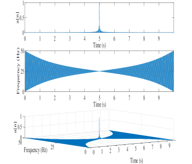
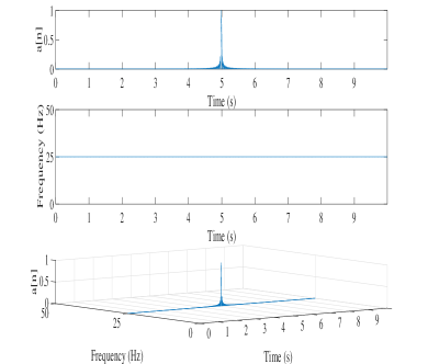
Figure 2: Analysis of unit sample sequence: time-amplitude (top), time-frequency (middle) and time-frequency-amplitude (bottom) subplots (a) and (b) obtained using the GAS and FSAS representations, respectively.

4.2 Chirp signal analysis

In this example, we consider an analysis of a non-stationary chirp signal using the proposed FSAS and compare the results with GAS approach, with sampling frequency $F_{s}=1000$ Hz, time duration $t\in[0,1)$ s and frequency $f\in[5,100)$ Hz. Figure 3 (a) shows chirp signal (5Hz–100Hz) (top), proposed FCQT (middle) obtained using (14) which is also imaginary part of the proposed FSAS (18), and HT (bottom) that is imaginary part of the GAS representation (3), which has unnecessary distortions at both ends of the signal. The TFE distributions obtained (1) using the FSAS representation is shown in Figure 3 (b), and (2) using the GAS representation is shown in Figure 3 (c), which has lot of energy spreading over wide range of time-frequency plane, at both ends of the signal under analysis. These examples, 4.1 and 4.2, clearly demonstrate the advantage of the proposed FSAS over the GAS representation for TFE analysis of a signal.

[]

[] []

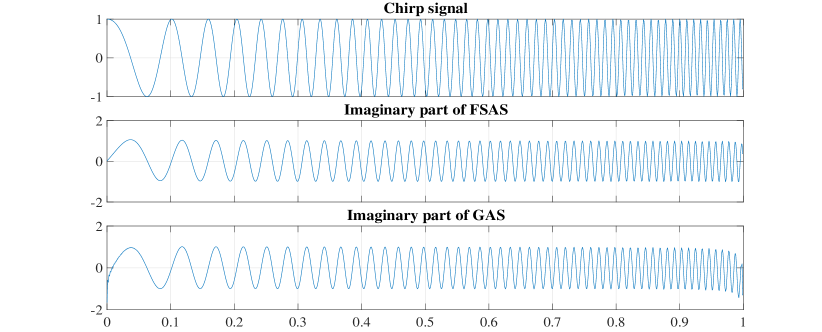
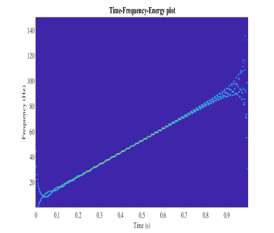
Figure 3: Analysis of a non-stationary signal: (a) A chirp signal (5Hz–100Hz) (top), FCQT–imaginary part of the proposed FSAS (middle), HT–imaginary part of GAS (bottom); obtained TFE representations using the FSAS (b), and GAS (c).

4.3 Speech signal analysis

An estimation of the instantaneous fundamental frequency $F_{0}$ is a most important problem in speech processing, because it arises in numerous applications, such as language identification [50], speaker recognition [51], emotion analysis [52], speech compression and voice conversion [53, 54]. Figure 4 (a) shows a segment of voiced speech signal (top) from CMU-Arctic database [49] sampled at $F_{s}=32000$ Hz, corresponding electroglottograph (EGG) signal (middle), and differenced EGG (bottom) signal. Figure 4 (b), top plot, shows magnitude spectrum of speech signal where $F_{0}$ is around 132 Hz, and energy of speech signal is concentrated on harmonics of $F_{0}$, and the magnitude spectrum of differenced EGG (DEGG) signal is shown in bottom plot that also indicate $F_{0}$ around 132 Hz. Figure 4 (c) shows a decomposition of speech segment into a set of nine FIBFs (FIBF1–FIBF9) and a low frequency component (LFC) using the FDM. Figure 4 (d) presents TFE representation obtained from the FDM where $F_{0}$ and its harmonics are clearly separated in distinct frequency bands. Thus, the FDM is able to achieve and follow the proposed model (7) precisely.

[] []

[] []

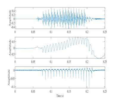
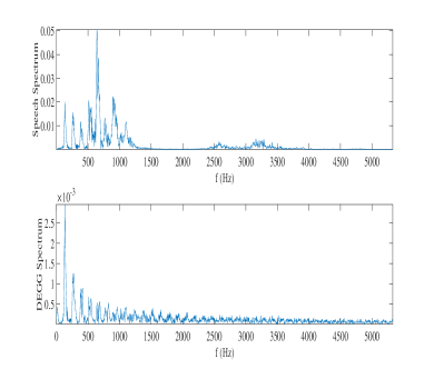
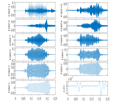
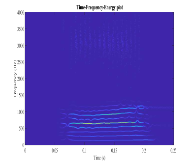
Figure 4: Analysis of speech signal: (a) A segment of speech (top), EEG (middle) and DEGG (bottom) signals, (b) Spectrum fo speech (top) and DEGG (bottom) signals, (c) Set of FIBFs obtained by the proposed DCT based FDM, and (d) TFE representation by proposed method.

4.4 Noise removal from ECG signal

Electrocardiogram (ECG) signals, records of the electrical activity of the heart, are used to examine the activity of human heart. There are various problems that may arise while recording an ECG signal. It may be distorted due to the presence of various noises such as channel noise, baseline wander (BLW) noise (of generally below 0.5 Hz), power-line interference (PLI) of 50 Hz (or 60 Hz), and physiological artifact. Due to these noises, it becomes difficult to diagnose diseases, and thus appropriate treatment may be impacted[55]. The BLW and PLI removal from an ECG signal (obtained from MIT-Arrhythmia database, $Fs=360$ Hz) using the proposed method is shown in Figure 5: (a) a segment of clean ECG signal (top), ECG signal heavily corrupted (i.e., SNR is low, in the range $\approx-18.4$ dB) with BLW and PLI (bottom) noises, (b) ECG signal after noise removal (top), separated BLW (middle) and PLI (bottom). Thus, proposed FDM can be used to remove BLW and PLI noises, and recover ECG signal even in scenarios where signal-to-noise ratio (SNR) is rather poor.

[] []

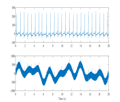
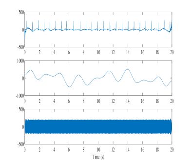
Figure 5: Noise removal from ECG signal using the proposed method: (a) A segment of clean ECG signal (top), ECG signal corrupted (SNR$\approx-18.4$ dB) with baseline wander and power-line interference (bottom), (b) ECG signal after noise removal (top), estimated baseline wander (middle) and power-line interference (bottom).

4.5 Trend and variability estimation from a nonlinear and nonstationary time series

Estimating trend and performing detrending operations are important steps in numerous applications, e.g., in climatic data analyses, the trend is one of the most critical parameters [57]; in spectral analysis and in estimating the correlation function, it is necessary to remove the trend from the data to obtain meaningful results [57]. Thus, in signal and other data analysis, it is crucial to estimate the trend, detrend the data, and obtain variability of the time series at any desired time scales.

The Global surface temperature anomaly (GSTA) data (of 148 Years from 1856 to 2003, publicly available at [56]) analysis and its trend obtained from the proposed method is shown in Figure 6: (a) GSTA data (blue solid), and its trend (red dashed, sixty four-years or longer time scale) obtained by dividing data into six dyadic frequency bands, and corresponding FIBFs (b). Figure 6 (c) obtained by decomposing the data into twelve FIBFs of non-dyadic frequency bands: FIBF11 shows (2–3) years time scale variations, FIBF10 (3–4), FIBF9 (4–6), FIBF8 (6–8), FIBF7 (8–12), FIBF6 (12–16), FIBF5 (16–24), FIBF4 (24–32), FIBF3 (32–44), FIBF2, (44–64), FIBF1 (64–80 years), and trend shows 80 years or longer time scale variations of temperature.

To demonstrate the efficacy of the proposed FDM to estimate a trend and variability from data at any desired time scale, e.g., we estimated the trends and variabilities of GSTA data in various time scales as shown in Figure 6 (d), Figure 7 and Figure 8. Figure 6 (d) shows GSTA data (blue solid), and trends (red dashed) in multiple of 10 (i.e. 10–80) years or longer time scale variations of temperature. Figure 7 presents: (a) GSTA data, and its trend in 15, 25 and 53 years or longer time scale, and (b) GSTA data, and its trend in 75, 100 and 125 years or longer time scale.

The variabilities of the annual GSTA data corresponding to various trends (i.e. data minus corresponding trends) with their time scales are given in Figure 8: (a) variabilities corresponding to trends in Figure 6 (d), and (b) variabilities corresponding to trends in Figure 7. From these Figures, it is clear that the variabilities up to 53 years or longer time scale are similar and don’t contain any low frequency component (i.e. there is no mode-mixing). However, the variabilities from 60 years (in fact experimentally found 54 years Figure 9) or longer time scale are different from up to 53 years and also contain low frequency component (i.e. there is mode-mixing).

The trend and variability analysis of this climate data is also performed by the EMD algorithm in [57]. The EMD algorithm decomposes the climate data into a set of IMFs which have overlapping frequency spectra and their cutoff frequencies are also not under control, therefore, the trend and variability of data at desired time scales with clear demarcation cannot be obtained. For example, we have shown that there is a significant change in the trend and variability of data in just one year difference of time scale (observe change in 53 years or longer time scale to 54 years or longer time scale in Figure 9). This kind of fine control along with determination of trend and variability of data in desired time scale with clear demarcation can be obtained by the proposed method, which is not achievable by the EMD and its related algorithms.

[] []

[] []

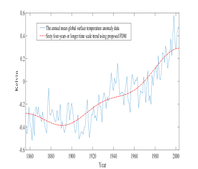
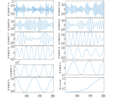
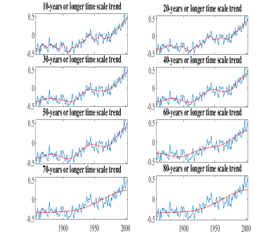
Figure 6: The GSTA data analysis using the proposed FDM: (a) GSTA data (blue solid), and its trend (red dashed) obtained by dividing data into six dyadic frequency bands, and corresponding dyadic FIBFs (b), (c) FIBFs obtained by dividing data into twelve non-dyadic frequency bands, and (d) GSTA data (blue solid) and trends (red dashed) in various time scales of 10–80 years or longer.

[] []

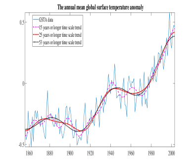
Figure 7: Trend analysis of GSTA data using the proposed FDM: (a) GSTA data, and its trend in 15, 25 and 53 years or longer time scale, (b) GSTA data, and its trend in 75, 100 and 125 years or longer time scale.

[] []

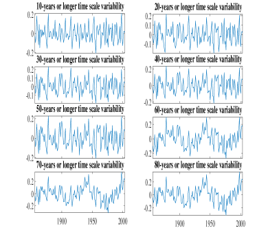
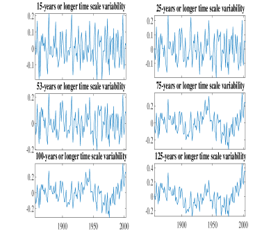
Figure 8: Variability analysis of GSTA data using the proposed FDM: (a) Variabilities in multiple of 10 (i.e. 10–80) years or longer time scales corresponding to trends in Figure 6 (d); and (b) Variabilities in 15, 25, 53, 75, 100, and 125 years or longer time scales.

[] []

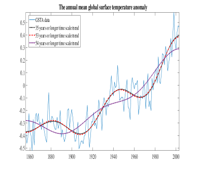
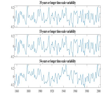
Figure 9: Trend and variability analysis of GSTA data using the proposed FDM: (a) GSTA data, and its trend in 35, 53 and 54 years or longer time scale, and (b) corresponding variabilities.

4.6 Seismic signal analysis

An Earthquake time series is nonlinear and nonstationary in nature and in this example we consider the Elcentro Earthquake data. The Elcentro Earthquake time series (which is sampled at $F_{s}=50$ Hz) has been downloaded from [46] and is shown in top Figure 10 (a). The most critical frequency range that matters in the structural design is less than $10$ Hz, and the Fourier power spectral density (PSD), bottom Figure 10 (a), shows that almost all the energy in this Earthquake time series is present within $10$ Hz. Figure 10 presents: (b) TFE distributions by the DCT based FDM method without decomposition, (c) FIBFs obtained by decomposing data into eight dyadic bands [FIBF0 (0–0.1953), FIBF1 (0.1953–0.390), FIBF2 (0.390–0.78125), FIBF3 (0.78125–1.5625), FIBF4 (1.5625–3.125), FIBF5 (3.125–6.25), FIBF6 (6.25–12.5), FIBF7 (12.5–25)] Hz, (d) ten equal energy FIBFs [FIBF0 (0–927.7344e-003), FIBF0 (927.7344e-003–1.1841), FIBF2 (1.1841–1.5015), FIBF3 (1.5015–1.8433), FIBF4 (1.8433–2.1606), FIBF5 (2.1606–2.6733), FIBF6 (2.6733–3.7109), FIBF7 (3.7109–4.7119), FIBF8 (4.7119–6.8237), FIBF9 (6.8237–25)] Hz, (e) TFE distribution corresponding eight dyadic bands, and (f) TFE distribution corresponding ten equal energy bands. The obtained TFE distributions indicate that the maximum energy in the signal is present around 2 second and 1.7 Hz. These FIBFs and TFE distributions provide details of how the different waves arrive from the epical center to the recording station, for example, the compression waves of small amplitude and higher frequency range 12 to 25 Hz [e.g. FIBF7 of Figure 10 (c)], the shear and surface waves of strongest amplitude and lower frequency range of below 12 Hz [e.g. FIBF6, FIBF5, FIBF4 and FIBF3 of Figure 10 (c)] which create most of the damage in structure, and other body shear waves of lowest amplitude and frequency range of below 1 Hz [e.g. FIBF2, FIBF1, and FIBF0 of Figure 10 (c)] which are present over the full duration of the time series.

[] []

[] []

[] []

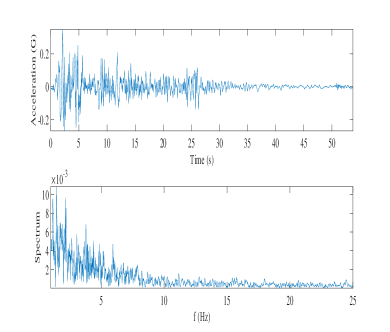
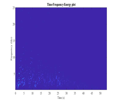
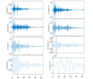
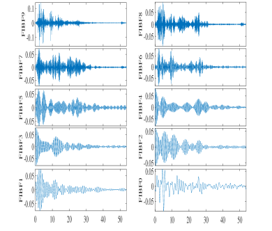
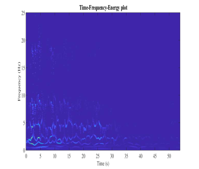
Figure 10: The Elcentro Earthquake (May 18, 1940) data analysis using the proposed FDM: (a) North-South component EQ data (top), and its Fourier spectrum (bottom), (b) TFE distribution without any decomposition, (c) FIBFs (8 dyadic frequency bands), (d) FIBFs (10 equal-energy frequency bands), (e) TFE corresponding to eight dyadic frequency bands, and (f) TFE corresponding to ten equal-energy frequency bands.

4.7 Gravitational wave event GW150914 analysis: Noise removal, IF and TFE estimation

Gravitational waves (GWs), predicted in 1916 by Albert Einstein, are ripples in the space-time continuum that travel outward from a source at the speed of light, and carry with them information about their source of origin. The GW event GW150914, produced by a binary black hole merger nearly 1.3 billion light years away [47], marks one of the greatest scientific discoveries in the history of human life. In this example, using the proposed method, we consider the noise removal, IF estimation and TFE representation of this GW event data which is publicly available at [48] (sampling rate $F_{s}=16384$ Hz). The GW signal sweeps upwards in frequency from 35 Hz to 250 Hz, and amplitude strain increases to a peak GW strain of $1.0\times 10^{-21}$ [47]. The noise removal and an accurate IF estimation of the GW data is important because IF is the basis to estimate many parameters such as velocity, separation, luminosity distance, primary mass, secondary mass, chirp mass, total mass, and effective spin of binary black hole merger [47]. Figure 11 shows (a) the GW H1 strain data GW150914 (top figure) observed at the laser interferometer gravitational-wave observatory (LIGO) Hanford which is heavily corrupted with noise, the Fourier spectrum (bottom figure) of the GW data which is not able to capture the non-stationarity (i.e. upwards sweep in the frequency and amplitude) present in the data, (b) the TFE representation of the GW H1 data by proposed method which shows the signal frequency is increasing with time but having lots of unnecessary fluctuations in frequency due to noise, and (c) decomposition of data into a set of six FIBFs [FIBF1 (25–60), FIBF2 (60–100), FIBF3 (100–200), FIBF4 (200–300), FIBF5 (300–350), FIBF6 (350–8192)] Hz and a low frequency component (LFC) 0–25 Hz), (d) FW1-FW5 are obtained by multiplying the time domain Gaussian window with corresponding FIBFs (FIBF1-FIBF5), and the reconstructed GW (RGW) is obtained by summation of FW1-FW5 components. In the reconstruction of wave, the LFC and FIBF6 have been ignored as they are out of band noises present in the GW H1 data.

The further analysis, comparison, residue and TFE estimation of GW event GW150914 H1 strain data (captured at LIGO Hanford) using the proposed FDM are shown in Figure 12: (a) GW H1 strain data (top red dashed line), proposed reconstruction (top blue solid line), and estimated residue component (bottom) (b) Numerical relativity (NR) data [47] (top red dashed line), and proposed reconstruction (top blue solid line), and difference between NR and reconstructed data (bottom); TFE estimates of the NR data and the reconstructed data are shown in (c) and (d), respectively. The very same analysis of the GW event GW150914 L1 strain data (captured at LIGO Livingston) using the proposed mythology is shown in Figure 13.

[] []

[] []

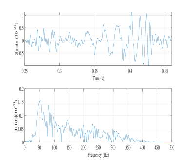
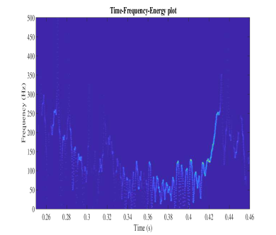
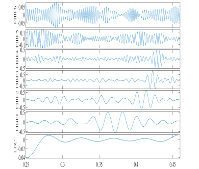
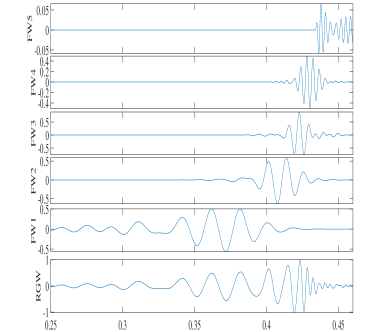
Figure 11: The GW event GW150914 H1 strain data (captured at LIGO Hanford) analysis using the proposed FDM: (a) The GW H1 strain data [47] (top figure), and its Fourier spectrum (bottom figure), (b) TFE estimates without any deposition, (c) obtained FIBF1-FIBF6 and low frequency component (LFC), (d) results (FW1-FW5) obtained by multiplication of FIBF1-FIBF6 with corresponding Gaussian windows, and reconstructed gravitational wave (RGW) by sum of FW1-FW5.

[] []

[] []

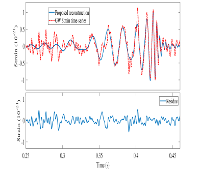
Figure 12: The GW event GW150914 H1 strain data analysis using the proposed FDM: (a) GW H1 strain data (top red dashed line), and proposed reconstruction (top blue solid line), and residue component (bottom) (b) Numerical relativity (NR) data (top red dashed line), and proposed reconstruction (top blue solid line), and difference between NR and reconstructed data (bottom), (c) TFE estimates of the NR data, and (d) TFE estimates of the reconstructed data.

[] []

[] []

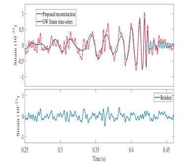
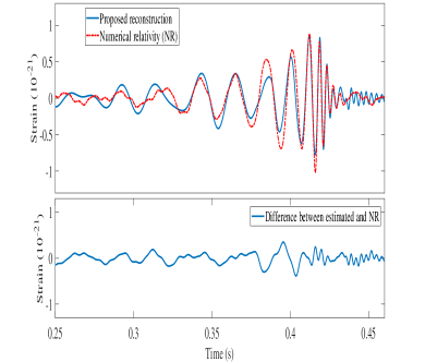
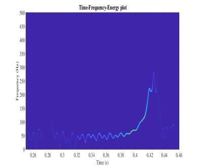
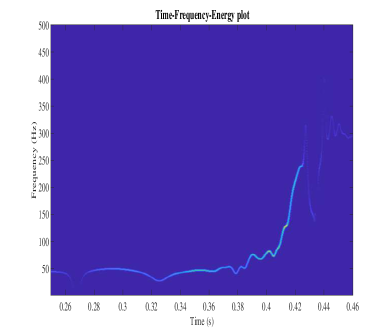
Figure 13: The GW event GW150914 L1 strain data (captured at LIGO Livingston) analysis using the proposed FDM: (a) GW L1 strain data (top red dashed line), and proposed reconstruction (top blue solid line), and residue component (bottom) (b) Numerical relativity (NR) data (top red dashed line), and proposed reconstruction (top blue solid line), and difference between NR and reconstructed data (bottom), (c) TFE estimates of the NR data, and (d) TFE estimates of the reconstructed data.

These examples clearly demonstrate the ability of the proposed method for the analysis of real-life nonstationary signals such as speech (Sec. 4.3), ECG (Sec. 4.4), climate (Sec. 4.5), seismic (Sec. 4.6) and gravitational (Sec. 4.7) time-series. This study is aimed to complement the current nonlinear and nonstationary data processing methods with the addition of the FDM based on the DCT, DCQT and zero-phase filter approach using GAS and FSAS representations.

5 Conclusion

The Hilbert transform (HT), to obtain quadrature component and Gabor analytic signal (GAS) representation, is most well-known and widely used mathematical formulation for modeling and analysis of signals in various applications. The fundamental contributions and conceptual innovations of this study are introduction of the new discrete Fourier cosine quadrature transforms (FCQTs) and discrete Fourier sine quadrature transforms (FCQTs), designated as Fourier quadrature transforms (FQTs), as effective alternatives to the HT. Using these FQTs, we proposed Fourier-Singh analytic signal (FSAS) representations, as alternatives to the GAS, with following properties: (1) real part of FSAS is the original signal and imaginary part is the FCQT of the real part, (2) imaginary part of FSAS is the original signal and real part is the FSQT of the real part, (3) like the GAS, Fourier spectrum of the FSAS has only positive frequencies, however unlike the GAS, the real and imaginary parts of the proposed FSAS representations are not orthogonal to each other. Continuous time FQTs, FSAS representations, and 2D extension of these formulations are also presented.

The Fourier theory and zero-phase filtering based Fourier decomposition method (FDM) is an adaptive data analysis approach to decompose a signal into a set of small number of Fourier intrinsic band functions (FIBFs). This study also proposed a new formulation of the FDM using the discrete cosine transform and the discrete cosine quadrature transform with the GAS and FSAS representations, and demonstrated its efficacy for analysis of nonlinear and non-stationary simulated as well as real-life time series such as instantaneous fundamental frequency estimation from unit sample sequence, chirp and speech signals, baseline wander and power-line interference removal from ECG data, trend and variability estimation and analysis of climate data, seismic time series analysis, and finally noise removal, IF and TFE estimation from the gravitational wave event GW150914 strain data.

Appendix A Continuous time Fourier Quadrature Transforms

The Fourier cosine transform (FCT) and inverse FCT (IFCT) pairs, of a signal, are defined as

$$X_{c}(\omega) =\sqrt{\frac{2}{\pi}}\int_{0}^{\infty}x(t)\cos(\omega t)\,\mathrm{d}t,\quad\omega\geq 0$$ (26)

$$x(t) =\sqrt{\frac{2}{\pi}}\int_{0}^{\infty}X_{c}(\omega)\cos(\omega t)\,\mathrm{d}\omega,\quad t\geq 0,$$

subject to the existence of the integrals, i.e., $x(t)$ is absolutely integrable ($\int_{0}^{\infty}|x(t)|\,\mathrm{d}t<\infty$) and its derivative $x^{\prime}(t)$ is piece-wise continuous in each bounded subinterval of $[0,\infty)$.

We hereby define the FCQT, $\tilde{x}_{c}(t)$, using the FCT of signal of $x(t)$ as

$$\tilde{x}_{c}(t)=\sqrt{\frac{2}{\pi}}\int_{0}^{\infty}X_{c}(\omega)\sin(\omega t)\,\mathrm{d}\omega={\frac{2}{\pi}}\int_{0}^{\infty}\left[\int_{0}^{\infty}x(\tau)\cos(\omega\tau)\,\mathrm{d}\tau\right]\sin(\omega t)\,\mathrm{d}\omega.$$ (27)

From (27), we obtain

$$\tilde{X}_{c}(\omega)=\sqrt{\frac{2}{\pi}}\int_{0}^{\infty}\tilde{x}_{c}(t)\sin(\omega t)\,\mathrm{d}t,$$ (28)

where

$$\tilde{X}_{c}(\omega)=\begin{cases}0,\quad\omega=0,\\ {X}_{c}(\omega),\quad\omega>0.\end{cases}$$ (29)

The proposed FSAS, using the FCQT, is defined as

$$\tilde{z}_{c}(t)=x(t)+j\tilde{x}_{c}(t)=\sqrt{\frac{2}{\pi}}\int_{0}^{\infty}X_{c}(\omega)\exp(j\omega t)\,\mathrm{d}\omega,$$ (30)

where real part is the original signal and imaginary part is the FQT of real part.

The Fourier sine transform (FST) and inverse FST (IFST) pairs, of a signal, are defined as

$$X_{s}(\omega) =\sqrt{\frac{2}{\pi}}\int_{0}^{\infty}x(t)\sin(\omega t)\,\mathrm{d}t,$$ (31)

$$x(t) =\sqrt{\frac{2}{\pi}}\int_{0}^{\infty}X_{s}(\omega)\sin(\omega t)\,\mathrm{d}\omega,$$

subject to the existence of the integrals. We hereby define the FSQT, $\tilde{x}_{s}(t)$, using the FST of signal of $x(t)$ as

$$\tilde{x}_{s}(t)=\sqrt{\frac{2}{\pi}}\int_{0}^{\infty}X_{s}(\omega)\cos(\omega t)\,\mathrm{d}\omega={\frac{2}{\pi}}\int_{0}^{\infty}\left[\int_{0}^{\infty}x(\tau)\sin(\omega\tau)\,\mathrm{d}\tau\right]\cos(\omega t)\,\mathrm{d}\omega.$$ (32)

From (32), we can write

$$\tilde{X}_{s}(\omega)=\sqrt{\frac{2}{\pi}}\int_{0}^{\infty}\tilde{x}_{s}(t)\cos(\omega t)\,\mathrm{d}t,$$ (33)

and one can observe that both representations, defined as FST of $x(t)$ in (31) and FCT of $\tilde{x}_{s}(t)$ in (33), are same for all frequencies, i.e. ${X}_{s}(\omega)=\tilde{X}_{s}(\omega)$.

The proposed FSAS, using the FSQT, is defined as

$$\tilde{z}_{s}(t)=\tilde{x}_{s}(t)+jx(t)=\sqrt{\frac{2}{\pi}}\int_{0}^{\infty}X_{s}(\omega)\exp(j\omega t)\,\mathrm{d}\omega,$$ (34)

where imaginary part is the original signal and real part is the FQT of imaginary part. The FQTs, presented in (27) and (32), are different from the HT by definition itself. The proposed FSAS representations, defined in (30) and (34), are effective alternatives to the GAS representation which is used in various applications such as envelop detection, IF estimation, time-frequency-energy representation and analysis of nonlinear and nonstationary data.

Appendix B The 2D DCT and corresponding FSAS representations

The 2D DCT-2 of a sequence, $x[n,m]$, is defines as [20]

$$X_{2}[k,l]=\frac{2}{\sqrt{MN}}\sum_{m=0}^{M-1}\sum_{n=0}^{N-1}\sigma_{k}\sigma_{l}x[m,n]\cos\left(\frac{\pi k(2m+1)}{2M}\right)\cos\left(\frac{\pi l(2n+1)}{2N}\right),$$ (35)

and IDCT is obtained by

$$x[m,n]=\frac{2}{\sqrt{MN}}\sum_{k=0}^{M-1}\sum_{l=0}^{N-1}\sigma_{k}\sigma_{l}{X_{2}[k,l]}\cos\left(\frac{\pi k(2m+1)}{2M}\right)\cos\left(\frac{\pi l(2n+1)}{2N}\right).$$ (36)

Using the relation, $\cos(\alpha)\cos(\beta)=\frac{1}{2}[\cos(\alpha+\beta)+\cos(\alpha-\beta)]$, we obtain the 2D FSAS as

$$\tilde{z}[m,n]=\frac{1}{\sqrt{MN}}\sum_{k=0}^{M-1}\sum_{l=0}^{N-1}\sigma_{k}\sigma_{l}{X_{2}[k,l]}\Big{[}\exp{\left(\frac{j\pi k(2m+1)}{2M}+\frac{j\pi l(2n+1)}{2N}\right)}\\ +\exp{\left(\frac{j\pi k(2m+1)}{2M}-\frac{j\pi l(2n+1)}{2N}\right)}\Big{]}=x[m,n]+j\tilde{x}[m,n],$$ (37)

where real part of (37) is the 2D original signal and imaginary of it is the 2D quadrature component of real part which can be written as, using $\sin(\alpha)\cos(\beta)=\frac{1}{2}[\sin(\alpha+\beta)+\sin(\alpha-\beta)]$,

$$\tilde{x}[m,n]=\frac{2}{\sqrt{MN}}\sum_{k=0}^{M-1}\sum_{l=0}^{N-1}\sigma_{k}\sigma_{l}{X_{2}[k,l]}\sin\left(\frac{\pi k(2m+1)}{2M}\right)\cos\left(\frac{\pi l(2n+1)}{2N}\right).$$ (38)

From (38), one can obtain

$${\tilde{X}_{2}[k,l]}=\frac{2}{\sqrt{MN}}\sum_{m=0}^{M-1}\sum_{n=0}^{N-1}\sigma_{k}\sigma_{l}\tilde{x}[m,n]\sin\left(\frac{\pi k(2m+1)}{2M}\right)\cos\left(\frac{\pi l(2n+1)}{2N}\right),$$ (39)

where

$${\tilde{X}_{2}[k,l]}=\begin{cases}0,\quad k=0,\,0\leq l\leq N-1,\\ {{X}_{2}[k,l]},\quad 1\leq k\leq M-1,\,0\leq l\leq N-1.\end{cases}$$ (40)

References

- [1] J. Carson, T. Fry, Variable frequency electric circuit theory with application to the theory of frequency modulation. Bell System Tech. J., 16, 513–540 (1937).
- [2] D. Gabor, Theory of communication, Electrical Engineers-Part III: Journal of the Institution of Radio and Communication Engineering, 93 (26), 429–441, (1946).
- [3] J. Ville, Theorie et application de la notion de signal analytic, Cables et Transmissions, 2A(1), 61–74, Paris, France, 1948. Translation by I. Selin, Theory and applications of the notion of complex signal, Report T-92, RAND Corporation, Santa Monica, CA.
- [4] J. Shekel, ‘Instantaneous’ frequency, Proc. IRE 41 (4), 548–548, (1953).
- [5] D.E. Vakman, On the definition of concepts of amplitude, phase and instantaneous frequency, Radio Eng. and Electron. Phys. 17, 754–759, (1972).
- [6] B. Boashash, Estimating and interpreting the instantaneous frequency of a signal–Part 1: Fundamentals. Proc. IEEE 80(4), 520–538 (1992).
- [7] B. Boashash, Estimating and interpreting the instantaneous frequency of a signal–Part 2: Algorithms and Applications. Proc. IEEE 80(4), 540–568 (1992).
- [8] L. Cohen, Time-Frequency Analysis, Prentice Hall, 1995.
- [9] P.J. Loughlin, B. Tacer, Comments on the Interpretation of Instantaneous Frequency. IEEE Signal Process. Lett. 4(5), 123–125 (1997).
- [10] N.E. Huang, Z. Shen, S. Long, M. Wu, H. Shih, Q. Zheng, N. Yen, C. Tung, H. Liu, The empirical mode decomposition and Hilbert spectrum for non-linear and non-stationary time series analysis. Proc. R. Soc. A, 454, 903–995, (1998).
- [11] B. Boashash, Time Frequency Signal Analysis and Processing: A Comprehensive Reference, Elsevier, Boston (2003).
- [12] S. Sandovala, P.L. De Leon, Theory of the Hilbert Spectrum, arXiv:1504.07554v4 [math.CV], 2015.
- [13] P. Singh, Breaking the Limits: Redefining the Instantaneous Frequency, Circuits Syst Signal Process (2017). https://doi.org/10.1007/s00034-017-0719-y.
- [14] P. Singh, provisional patent, lodged March 2018.
- [15] N. Ahmed, T. Natarajan, K.R. Rao, Discrete Cosine Transform, IEEE Trans. Computers, 90–93, (1974).
- [16] S.L. Marple, Computing the Discrete-Time Analytic Signal via FFT, IEEE Transactions on Signal Processing, 47 (9), 2600–2603, (1999).
- [17] J.P. Princen, A.W. Johnson, A.B. Bradley, Subband/transform coding using filter bank designs based on time domain aliasing cancellation, IEEE Proc. Intl. Conference on Acoustics, Speech, and Signal Processing (ICASSP), 2161–2164, (1987).
- [18] J.P. Princen, A.B. Bradley, Analysis/synthesis filter bank design based on time domain aliasing cancellation, IEEE Trans. Acoust. Speech Signal Processing, ASSP-34 (5), 1153–1161, (1986).
- [19] Gupta A., Singh P., Karlekar M., A novel Signal Modeling Approach for Classification of Seizure and Seizure-free EEG Signals, IEEE Transactions on Neural Systems and Rehabilitation Engineering, DOI: 10.1109/TNSRE.2018.2818123, 2018.
- [20] V. Britanak, P.C. Yip, K.R. Rao, Discrete Cosine and Sine Transforms: General properties, Fast algorithms and Integer Approximations, February 2006.
- [21] Z. Wu, N.E. Huang, Ensemble Empirical Mode Decomposition: a noise-assisted data analysis method. Adv. Adapt. Data Anal., 1 (1), 1–41, (2009).
- [22] N. Rehman, D.P. Mandic, Multivariate empirical mode decomposition. Proc. R. Soc. A, 466, 1291–1302. (2010).
- [23] P. Singh, S.D. Joshi, R.K. Patney, K. Saha, The Hilbert spectrum and the Energy Preserving Empirical Mode Decomposition. arXiv:1504.04104 [cs.IT], (2015).
- [24] P. Singh, S.D. Joshi, R.K. Patney, K. Saha, Some studies on nonpolynomial interpolation and error analysis. Appl. Math. Comput. 244, 809–821 (2014).
- [25] P. Singh, P.K. Srivastava, R.K. Patney, S.D. Joshi, K. Saha, Nonpolynomial spline based empirical mode decomposition. Signal Processing and Communication (ICSC), 2013 International Conference on, 435–440, (2013).
- [26] W.X. Yang, Interpretation of mechanical signals using an improved Hilbert–Huang transform. Mech. Syst. Signal Process. 22, 1061–1071 (2008)
- [27] Z. He, Q. Wang, Y. Shen, M. Sun, Kernel Sparse Multitask Learning for Hyperspectral Image Classification With Empirical Mode Decomposition and Morphological Wavelet-Based Features. IEEE Trans. Geosci. Remote Sens. 52(8), 5150–5163 (2014)
- [28] B. Demir, S. Erturk, Empirical Mode Decomposition of Hyperspectral Images for Support Vector Machine Classification. IEEE Trans. Geosci. Remote Sens. 48(11), 4071–4084 (2010)
- [29] P. Singh, S.D. Joshi, R.K. Patney, K. Saha, The Linearly Independent Non Orthogonal yet Energy Preserving (LINOEP) vectors. arXiv:1409.5710 [math.NA], (2014).
- [30] I. Daubechies, J. Lu, H.T. Wu, Synchrosqueezed Wavelet Transforms: an Empirical Mode Decomposition-like Tool. Appl. Comput. Harmon. Anal., 30, 243–261, (2011).
- [31] K. Dragomiretskiy, D. Zosso, Variational Mode Decomposition. IEEE Trans. Signal Process. 62(3), 531–544 (2014)
- [32] P. Jain, R.B. Pachori, An iterative approach for decomposition of multi-componentnon-stationary signals based on eigenvalue decomposition of the Hankel matrix. J. Franklin Inst. 352(10), 4017–4044, (2015).
- [33] J. Gilles, Empirical Wavelet Transform. IEEE Trans. Signal Process. 61(16), 3999–4010, (2013).
- [34] P. Singh, Some studies on a generalized Fourier expansion for nonlinear and nonstationary time series analysis. PhD thesis, Department of Electrical Engineering, IIT Delhi, India (2016).
- [35] S. Meignen, V. Perrier, A new formulation for empirical mode decomposition based on constrained optimization. IEEE Signal Process. Lett. 14(12), 932–935, (2007).
- [36] T.Y. Hou, Z. Shi, Adaptive data analysis via sparse time-frequency representation. Adv. Adapt. Data Anal. 3(1&2), 1–28, (2011).
- [37] M. Feldman, Time-varying vibration decomposition and analysis based on the Hilbert transform. J. Sound Vibrat. 295(3–5), 518–530, (2006).
- [38] I.W. Selesnick, Resonance-based signal decomposition: A new sparsity-enabled signal analysis method. Signal Process. 91(12), 2793–2809, (2011).
- [39] P. Singh, S.D. Joshi, R.K. Patney, K. Saha, The Fourier decomposition method for nonlinear and non-stationary time series analysis. Proc. R. Soc. A 20160871 (2017). http://dx.doi.org/10.1098/rspa.2016.0871.
- [40] P. Singh, Time-Frequency analysis via the Fourier Representation. arXiv:1604.04992 [cs.IT], (2016).
- [41] D.A. Cummings, R.A. Irizarry, N.E. Huang, T.P. Endy, A. Nisalak, K. Ungchusak, D.S. Burke, Travelling waves in the occurrence of dengue haemorrhagic fever in Thailand. Nature. 427, 344–347 (2004)
- [42] P. Singh, S.D. Joshi, Some studies on multidimensional Fourier theory for Hilbert transform, analytic signal and space-time series analysis. arXiv:1507.08117 [cs.IT], (2015).
- [43] P. Singh, LINOEP vectors, spiral of Theodorus, and nonlinear time-invariant system models of mode decomposition. arXiv:1509.08667 [cs.IT], (2015).
- [44] P. Singh, S.D. Joshi, R.K. Patney, K. Saha, Fourier-based Feature Extraction for Classification of EEG Signals Using EEG Rhythms. Circuits Syst. Signal Process. 35(10), 3700–3715 (2016).
- [45] B. Van der Pol, The fundamental principles of frequency modulation, Proc. IEE. 93(111), 153–158 (1946)
- [46] [Online:] http://www.vibrationdata.com/elcentro.htm
- [47] B.P. Abbott et al., Observation of Gravitational Waves from a Binary Black Hole Merger. Phys. Rev. Lett. PRL 116, 061102 (1–16) (2016).
- [48] https://losc.ligo.org/events/GW150914/
- [49] J. Kominek, A. W. Black, The CMU Arctic speech databases, in Fifth ISCA Workshop on Speech Synthesis, 2004.
- [50] H. Li, B. Ma, and C.-H. Lee, A vector space modeling approach to spoken language identification, IEEE Transactions on Audio, Speech, and Language Processing, vol. 15. no. 1, pp. 271–284, 2007.
- [51] E. Shriberg, L. Ferrer, S. Kajarekar, A. Venkataraman, and A. Stolcke, Modeling prosodic feature sequences for speaker recognition, Speech Commun., vol. 46, no. 34, pp. 455-472, Jul. 2005.
- [52] A. Tawari and M. Trivedi, Speech emotion analysis in noisy real-world environment, in Proc. Int. Conf. Pattern Recogn., Aug. 2010, pp. 4605-4608.
- [53] R. Taori, R. J. Sluijter, and E. Kathmann, Speech compression using pitch synchronous interpolation, in Proc. IEEE Int. Conf. Acoust. Speech, Signal Process, May 1995, vol. 1, pp. 512-515.
- [54] K. S. Rao, Voice conversion by mapping the speaker-specific features using pitch synchronous approach, Comput. Speech Lang., vol. 24, no. 3, pp. 474-494, Jul. 2010.
- [55] Agrawal, S., Gupta, A., Fractal and EMD based removal of baseline wander and powerline interference from ECG signals, Computers in biology and medicine, 43(11), 1889–1899, 2013.
- [56] http://rcada.ncu.edu.tw/research1_clip_ex.htm.
- [57] Wu Z., Huang N.E., Long S.R., Peng C.K., On the trend, detrending, and variability of nonlinear and nonstationary time series, Proc Natl Acad Sci USA, 104(38) 14889–14894, 2007.