Adaptive sampling of large deviations

Abstract

We introduce and test an algorithm that adaptively estimates large deviation functions characterizing the fluctuations of additive functionals of Markov processes in the long-time limit. These functions play an important role for predicting the probability and pathways of rare events in stochastic processes, as well as for understanding the physics of nonequilibrium systems driven in steady states by external forces and reservoirs. The algorithm uses methods from risk-sensitive and feedback control to estimate from a single trajectory a new process, called the driven process, known to be efficient for importance sampling. Its advantages compared to other simulation techniques, such as splitting or cloning, are discussed and illustrated with simple equilibrium and nonequilibrium diffusion models.

I Introduction

We consider in this paper the problem of estimating large deviation functions characterizing the fluctuations of time-integrated functionals of Markov processes in the long-time limit. These functions have a wide range of applications in engineering and physical sciences, where they are used to predict the probability of rare events Shwartz and Weiss (1995); Dembo and Zeitouni (1998); den Hollander (2000) and to understand how these events arise via transition paths or modified processes Jack and Sollich (2010); Chetrite and Touchette (2013, 2015a). Large deviation theory also underlies now much of the research on nonequilibrium systems driven in steady states by non-conservative forces or boundary reservoirs Touchette (2009); Derrida (2007); Harris and Touchette (2013). In this context, large deviation functions play the role of nonequilibrium potentials, similar to the entropy or free energy, that characterize the steady state and fluctuations of physical quantities, such as energy or particle currents exchanged with reservoirs, as well as the presence of symmetries Harris and Schütz (2007) and phase transitions in fluctuations Garrahan et al. (2007); Hedges et al. (2009); Espigares et al. (2013); Aminov et al. (2014).

Recently, many efforts have been devoted to developing numerical algorithms for estimating large deviation functions that go beyond the direct sampling of probabilities, which require prohibitively large samples. The most popular algorithms are variations of two basic approaches used in rare event simulations, namely: 1) splitting Dean and Dupuis (2009); Cérou and Guyader (2007); Aristoff et al. (2015) or cloning Grassberger (2002); Giardina et al. (2006); Lecomte and Tailleur (2007) algorithms, which use population dynamics to estimate probabilities or generating functions that have a multiplicative structure in time, and 2) importance sampling Bucklew (2004); Juneja and Shahabuddin (2006); Asmussen and Glynn (2007) (including transition path sampling Bolhuis et al. (2002)), which modifies the process to be simulated, so as to transform rare events into typical events that can be simulated efficiently. Deterministic methods not based a priori on sampling can also be used, including spatial discretizations of various spectral and optimal control representations of large deviation functions, which work well for low-dimensional systems, in addition to action minimization methods, which can be applied in the low-noise or low-temperature limit Heymann and Vanden Eijnden (2008); Vanden-Eijnden and Weare (2012); Grafke et al. (2015).

In this paper, we propose an algorithm that combines spectral methods with importance sampling to efficiently estimate large deviation functions in an adaptive way. The core of the algorithm comes from recent works on learning algorithms for risk-sensitive control of Markov chains Borkar et al. (2004); Ahamed et al. (2006); Basu et al. (2008); Borkar (2010), which we adapt to continuous-time diffusion processes and to the problem of estimating large deviation functions. The algorithm works by estimating or learning “on the fly” a modified process, called the auxiliary or driven process, which corresponds to the process that is asymptotically equivalent to the original process conditioned on the rare event of interest Chetrite and Touchette (2015a) or, alternatively, to the exponential tilting of the original process, known to be efficient for importance sampling Chetrite and Touchette (2015b). This modified process is given by a principal eigenvalue problem related to the Feynman–Kac equation or, equivalently, by a stochastic optimal control problem Chetrite and Touchette (2015b) that we solve iteratively using stochastic approximation and feedback control methods.

The main advantage of this algorithm, compared to splitting or cloning, is that it does not require the simulation of many copies of the process considered – it runs on one long trajectory of that process, modified with a feedback-reinforcement rule, to adaptively learn the driven process, thereby reducing significantly the complexity of estimating large deviation functions. The calculation of error bars for the estimated quantities is also simplified compared to other techniques, as the algorithm is based on simple time averages and stochastic approximations Chauveau and Diebolt (2003); Roberts and Rosenthal (2004); Benveniste et al. (2012). Finally, the errors incurred by discretizing continuous-time processes and functionals can be analysed in a precise way, in principle, via Feynman–Kac semi-groups Ferré and Stoltz (2017).

We discuss these advantages and test the algorithm in Sec. IV with simple equilibrium and nonequilibrium diffusions, after introducing the general model and notations in Sec. II and the algorithm in Sec. III. The results at this point are preliminary and are presented as a proof of concept of the algorithm. More detailed results about the time-discretization and sampling errors will be addressed in future works, together with more complex applications involving interacting particle systems and higher-dimensional diffusions.

II Framework

II.1 Model and notations

We consider an ergodic diffusion $(X_{t})_{t\geq 0}$ evolving in a state space $\mathcal{X}\subset\mathbb{R}^{d}$ according to the following stochastic differential equation (SDE):

$$dX_{t}=b(X_{t})\,dt+\sigma\,dW_{t},$$ (1)

where $b:\mathcal{X}\to\mathbb{R}^{d}$ is a smooth function, called the drift, $W_{t}$ is an $m$-dimensional Brownian motion, and $\sigma$ is a $d\times m$ matrix, assumed to be constant for simplicity. The generator of this diffusion reads

$$L=b\cdot\nabla+\frac{1}{2}\nabla\cdot D\nabla,$$ (2)

where $\cdot$ denotes the scalar product and $D=\sigma\sigma^{\mathsf{T}}$, with $\mathsf{T}$ as the transpose, is the diffusion matrix, assumed to be positive definite. This is the generator of the evolution semi-group $P_{T}$, defined by

$$P_{T}\varphi(x)=\mathbb{E}\left[\varphi(X_{T})\,\middle|\,X_{0}=x\right],$$ (3)

for all time $T\geq 0$ and any smooth test function $\varphi$. The dual $L^{\dagger}$ of $L$ in the space $L^{2}(dx)$ of square-integrable functions with respect to the Lebesgue measure is the generator of the Fokker-Planck equation

$$\partial_{t}\rho(x,t)=L^{\dagger}\rho(x,t),$$ (4)

which gives the evolution of the probability density $\rho(\cdot,t)$ of $X_{t}$ starting from some initial density $\rho(\cdot,0)$ for $X_{0}$.

Our goal here is to study the fluctuations of time-integrated functionals of $X_{t}$, called observables, having the general form

$$A_{T}=\frac{1}{T}\int_{0}^{T}f(X_{t})\,dt+\frac{1}{T}\int_{0}^{T}g(X_{t})\circ dX_{t},$$ (5)

where $f:\mathcal{X}\to\mathbb{R}$ and $g:\mathcal{X}\to\mathbb{R}^{d}$ are reasonably smooth functions (e.g. continuous) and $\circ$ denotes the Stratonovich product Pavliotis (2014). Such a functional defined over the time horizon $[0,T]$ can represent, for example, a control cost associated with the state $X_{t}$ and its increments Chernyak et al. (2014) or a physical quantity integrated in time, such as the work performed on a particle by external forces or the heat exchanged by a particle with its environment Sekimoto (2010).

Assuming that the process is ergodic with respect to an invariant measure $\mu(dx)=\rho^{*}(x)\,dx$ with smooth density $\rho^{*}$, we have

$$A_{T}\xrightarrow{T\to\infty}\int_{\mathcal{X}}f(x)\rho^{*}(x)\,dx+\int_{\mathcal{X}}g(x)\cdot J^{*}(x)\,dx=a^{*},$$ (6)

almost surely, where

$$J^{*}(x)=b(x)\rho^{*}(x)-\frac{D}{2}\nabla\rho^{*}(x)$$ (7)

is the stationary current field associated with $\rho^{*}$ Chetrite and Touchette (2015b). The theory of large deviations Dembo and Zeitouni (1998) refines this ergodic theorem, generalized here with the additional $g$ term, by providing estimates for the rate at which the probability distribution of $A_{T}$ concentrates on its ergodic value $a^{*}$. Such estimates can be derived under general conditions (see Dembo and Zeitouni (1998)) and take, in the simplest case, the form

$$\lim_{T\rightarrow\infty}-\frac{1}{T}\log\mathbb{P}(A_{T}\in B)=\min_{a\in B}\,I(a),$$ (8)

for any Borel subset $B$ of $\mathbb{R}$, where $I:\mathbb{R}\rightarrow\mathbb{R}_{+}$ is a positive function such that $I(a^{*})=0$. When this limit exists, $A_{T}$ is said to satisfy the large deviation principle (LDP) with rate function $I$. Formally, this means that

$$\mathbb{P}(A_{T}\in da)=\mathrm{e}^{-TI(a)+o(T)}da,$$ (9)

where $o(T)$ denotes corrections in the exponential that grow slower than linearly in $T$. Thus, we see that the rate function provides useful information about the fluctuations of $A_{T}$: the likelihood that $A_{T}=a$ decays exponentially with time for all $a\neq a^{*}$, since $I(a)>0$ in this case, and converges otherwise to 1 as $T\rightarrow\infty$, since $I(a^{*})=0$. Moreover, the rate function is in general not a parabola, meaning that it describes fluctuations that are generally not Gaussian. In this sense, large deviation theory is often seen as an extension of both the ergodic theorem, which describes the concentration of $A_{T}$ towards its mean, and the central limit theorem, which describes the local Gaussian fluctuations of $A_{T}$ around its mean Dembo and Zeitouni (1998).

II.2 Large deviation functions and driven process

In practice, the rate function $I(a)$ can be calculated in many different ways other than by direct sampling, which requires exponentially large samples with $T$ Bucklew (2004). The most common method proceeds from the scaled cumulant generating function (SCGF), defined for $k\in\mathbb{R}$ by

$$\lambda(k)=\underset{T\rightarrow\infty}{\lim}\ \frac{1}{T}\log\mathbb{E}\left[\mathrm{e}^{kTA_{T}}\right].$$ (10)

By the Gärtner-Ellis Theorem Dembo and Zeitouni (1998), the Legendre–Fenchel transform of this function yields the rate function:

$$I(a)=\sup_{k\in\mathbb{R}}\,\{ka-\lambda(k)\},$$ (11)

provided, essentially, that $\lambda(k)$ is differentiable; see Dembo and Zeitouni (1998) for more precise conditions.

For the SDE (1) and the additive functional (5), the SCGF is known to be given by the principal eigenvalue of the operator

$$\mathcal{L}_{k}=b\cdot(\nabla+kg)+\frac{1}{2}(\nabla+kg)\cdot D(\nabla+kg)+kf,$$ (12)

which is the generator of the Feynman–Kac semi-group $P_{T}^{k}$, defined by

$$P_{T}^{k}\varphi(x)=\mathbb{E}\left[\varphi(X_{T})\,\mathrm{e}^{TkA_{T}}\,\middle|\,X_{0}=x\right],$$ (13)

for any smooth function $\varphi$; see Appendix A.2 of Chetrite and Touchette (2015a). In the end, the rate function can thus be computed by solving the spectral problem

$$\mathcal{L}_{k}h_{k}=\lambda(k)h_{k},$$ (14)

where $\lambda(k)$ is the principal eigenvalue of $\mathcal{L}_{k}$ and $h_{k}$ its corresponding eigenvector. This holds provided that this operator has reasonable spectral properties, made precise in the following assumption.

Assumption 1.

The operator $\mathcal{L}_{k}$ defined in (12) acting on $L^{2}(\mu)$ has an isolated largest eigenvalue $\lambda(k)$. Its multiplicity is one and it is associated with a regular eigenvector $h_{k}\in L^{2}(\mu)$ such that for all $x\in\mathcal{X}$, $h_{k}(x)>0$.

This assumption holds for many systems, in particular when $\mathcal{X}$ is bounded Bierkens et al. (2016); Ferré and Stoltz (2017) or when $b$ and $g$ are gradient fields with appropriate growth conditions; see (Lelièvre and Stoltz, 2016, Sec. 2.5). In practice, the spectral problem (14) can be solved numerically using standard projection or discretization (Galerkin) methods, which work well for low-dimensional systems Chatelin (2011), or more involved real space renormalization methods when dealing with higher-dimensional systems Gorissen and Vanderzande (2011). Note that, for $g=0$, $\mathcal{L}_{k}$ is the usual Feynman–Kac generator with source term $kf$. Moreover, for $k=0$, $\mathcal{L}_{0}=L$ is the generator of the SDE, so that $\lambda(0)=0$ and $h_{0}=1$, the constant unit function.

The numerical method that we propose in the next section attempts to estimate the spectral elements $\lambda(k)$ and $h_{k}$ in a different way using the fact that they are solutions of the family of eigenproblems

$$P_{T}^{k}h_{k}=\mathrm{e}^{T\lambda(k)}h_{k},\qquad\forall\,T>0,$$ (15)

which can be approximated stochastically. The method also exploits a connection between large deviations and control theory showing that $\lambda(k)$ is the ergodic limit of an optimal control cost satisfying a stochastic Hamilton–Jacobi–Bellman equation Fleming and Soner (2006), and that $h_{k}$ determines the controlled diffusion achieving the optimal cost, which is the driven process mentioned in the introduction. These results are explained in detail in Chetrite and Touchette (2015b) (see also references therein); for the purpose of this paper, we only state them without proofs.

The controlled diffusion, denoted by $(\tilde{X}_{t})_{t\geq 0}$, satisfies the SDE

$$d\tilde{X}_{t}=b_{k}(\tilde{X}_{t})\,dt+\sigma\,dW_{t},$$ (16)

where

$$b_{k}(x)=b(x)+D[kg(x)+\nabla\log h_{k}(x)]$$ (17)

is the optimal control drift defined for all $x\in\mathcal{X}$. Under Assumption 1, this modified diffusion is ergodic with respect to a new invariant measure $\mu_{k}$, whose density is

$$\rho_{k}(x)=h_{k}(x)l_{k}(x),$$ (18)

where $l_{k}$ is the dual of $h_{k}$ in $L^{2}(dx)$ satisfying $\mathcal{L}_{k}^{\dagger}l_{k}=\lambda(k)l_{k}$ (Chetrite and Touchette, 2015a, Sec. 3.3). These two functions are normalized such that

$$\int_{\mathcal{X}}h_{k}(x)l_{k}(x)\,dx=1,\qquad\int_{\mathcal{X}}l_{k}(x)\,dx=1.$$ (19)

Because of the change of process, the observable $A_{T}$ must concentrate on a new value, which can be shown to be given by $\lambda^{\prime}(k)$, that is,

$$A_{T}\xrightarrow{T\to\infty}\lambda^{\prime}(k)=a_{k},$$ (20)

almost surely with respect to $(\tilde{X}_{t})_{t\geq 0}$. Similarly, the control cost

$$C_{T}=kA_{T}-R_{T},$$ (21)

where

$$R_{T}=\frac{1}{2T}\int_{0}^{T}[b(\tilde{X}_{t})-b_{k}(\tilde{X}_{t})]\cdot D^{-1}[b(\tilde{X}_{t})-b_{k}(\tilde{X}_{t})]\,dt,$$ (22)

reaches in the ergodic limit the value $\lambda(k)$, so that

$$C_{T}\xrightarrow{T\to\infty}\lambda(k)$$ (23)

almost surely under $(\tilde{X}_{t})_{t\geq 0}$ (Chetrite and Touchette, 2015b, Sec. 4). Finally, it can be shown by Legendre duality that the rate function at the value $a_{k}=\lambda^{\prime}(k)$ is given by the ergodic limit of $R_{T}$ above, leading to

$$R_{T}\xrightarrow{T\to\infty}I(a_{k}),$$ (24)

almost surely with respect to $(\tilde{X}_{t})_{t\geq 0}$ (Chetrite and Touchette, 2015b, Sec. 4). Note that the diffusion is not modified for $k=0$, so that $a_{0}=a^{*}$, $\lambda^{\prime}(0)=a^{*}$, and $I(a^{*})=0$.

These ergodic limits provide direct estimators of the SCGF and the rate function, based on a single trajectory of the driven process, which can be simulated for different values of the parameter $k\in\mathbb{R}$. For the SCGF, there are in fact three possible estimators:

1. From (20): The value of $A_{T}$, integrated numerically with the condition $\lambda(0)=0$.

2. From (23): The value of $C_{T}$.

3. The eigenvalue returned by the algorithm proposed in Sec. III.

In practice, we find that the last estimator is more stable, although the first and second are more adapted to obtain error bars.

For the rate function, we have two possible estimators:

1. The Legendre transform (11) of the SCGF, given in parametric form by

   $$I(a_{k})=ka_{k}-\lambda(k),$$ (25)

   where $a_{k}$ is either estimated from $A_{T}$ or by taking the numerical derivative of $\lambda(k)$.

2. From (24): The value of $R_{T}$ obtained for the value of $A_{T}$, giving the couple $(A_{T},R_{T})$.

In practice, we find that the first estimator based on the Legendre transform is more reliable. By comparison, the computation of $I(a)$ based on (22) involves the optimal drift $b_{k}$ and, therefore, the logarithmic derivative of $h_{k}$, which is more difficult to estimate in a stable way.

In all cases, error bars can be constructed from the same trajectory by estimating, in principle, the variance of $A_{T}$, $C_{T}$ and $R_{T}$ using covariance techniques for Markov processes Chauveau and Diebolt (2003); Roberts and Rosenthal (2004); Benveniste et al. (2012). This is an advantage over splitting and cloning algorithms, for which the calculation of errors bars is difficult, as they involve correlated copies or “clones” of the simulated process Rousset (2006); Nemoto et al. (2016, 2017a).

In closing, it is interesting to note that the driven process can also be interpreted as the change of process in the importance sampling of the probability $\mathbb{P}(A_{T}\in B)$ that is optimal in the sense of logarithmic or asymptotic efficiency Bucklew (2004). Therefore, it can be used not only to estimate the SCGF and rate function, but also to estimate the actual probability $\mathbb{P}(A_{T}\in B)$ in an efficient way Borkar et al. (2004). The optimal change of process in this case is known to correspond to the exponential tilting of the original process Bucklew (2004), which is a time-dependent process in general; see Appendix D of Chetrite and Touchette (2015a). In the ergodic limit, this process converges to a homogeneous process corresponding exactly to the driven process (16). We refer to Chetrite and Touchette (2015b) for more details about these results.

III Adaptive algorithm

We are now ready to present the algorithm for estimating the SCGF and the rate function of $A_{T}$ for continuous-time diffusions. The algorithm is based, as mentioned, on prior algorithms proposed in Borkar et al. (2004); Ahamed et al. (2006); Basu et al. (2008); Borkar (2010) for Markov chains and exploits the fact that

$$\mathrm{e}^{-T\lambda(k)}(P_{T}^{k}\varphi)\xrightarrow{T\to\infty}h_{k}\int_{\mathcal{X}}\varphi(x)\,l_{k}(x)\,dx,$$ (26)

for any smooth test function $\varphi$. This result follows under Assumption 1; see (Chetrite and Touchette, 2015a, Sec. III.B) or (Ferré and Stoltz, 2017, Sec. 6.1) for a proof. The algorithm that we propose works from this limit by approximating the action of the Feynman–Kac semi-group $P_{T}^{k}$ in a stochastic way as a time average computed over a long trajectory of the diffusion. Moreover, it continuously modifies the diffusion as we estimate $h_{k}$ to construct the driven process $(\tilde{X}_{t})_{t\geq 0}$, which underlies the estimators of the large deviation functions.

The algorithm is presented next. Our contribution compared to Borkar et al. (2004); Ahamed et al. (2006); Basu et al. (2008); Borkar (2010) is to consider general time-continuous processes, time-additive functionals of these processes that depend on both their state and increments, and, more importantly, to construct the driven process explicitly so as to estimate the SCGF and the rate function adaptively using the estimators introduced in the previous section.

III.1 Time discretization

The first step required in the algorithm is to discretize in time the SDE (1) and its associated Feynman–Kac semi-group (13) by transforming the Markov diffusion $(X_{t})_{t\geq 0}$ into a Markov chain $(x_{n})_{n\in\mathbb{N}}$ with a small time step. Many discretization schemes can be used for the SDE; see, for instance, Kloeden and Platen (1992). Here we use the standard Euler–Maruyama scheme with constant time step $\Delta t$, given by

$$x_{n+1}=x_{n}+b(x_{n})\Delta t+\sigma\sqrt{\Delta t}\,\xi_{n},$$ (27)

where $(\xi_{n})_{n\geq 0}$ is a sequence of independent standard $d$-dimensional Gaussian random variables. The corresponding discretization of the evolution semi-group $P_{T}$ over a time step $\Delta t$ is denoted by $Q_{\Delta t}$, so that

$$Q_{\Delta t}\varphi(x)=\mathbb{E}\left[\varphi(x_{n+1})\middle|x_{n}=x\right],$$ (28)

for any test function $\varphi$ and $x\in\mathcal{X}$. We refer to Kloeden and Platen (1992); Lelièvre and Stoltz (2016) for more information about the discretization of SDEs and their weak error analysis.

Many discretizations also exist for the Feynman–Kac semi-group $P_{T}^{k}$. Here, we use the natural scheme where the diffusion is discretized as above and the integral of $A_{T}$ is discretized as a Riemann sum with the left-point rule for the integral involving $f$ and the mid-point rule for the Stratonovich integral involving $g$ Ferré and Stoltz (2017). The action of $P_{T}^{k}$ is thus replaced by

$$Q_{\Delta t}^{k}\varphi(x)=\mathbb{E}\left[\mathrm{e}^{k\left[f(x_{n})\Delta t+g\left(\frac{x_{n+1}+x_{n}}{2}\right)\cdot(x_{n+1}-x_{n})\right]}\varphi(x_{n+1})\ \middle|\ x_{n}=x\right].$$ (29)

For our purposes, $h_{k}$ will be approximated by recursive applications of $Q_{\Delta t}^{k}$, based on the following assumption.

Assumption 2.

There exist a time step $\Delta t^{*}>0$ and $p>0$ such that, for $0<\Delta t\leq\Delta t^{*}$,

$$Q_{\Delta t}^{k}h_{k,\Delta t}=\mathrm{e}^{\Delta t\lambda_{\Delta t}(k)}h_{k,\Delta t},$$ (30)

where

$$h_{k,\Delta t}=h_{k}+O(\Delta t^{p}),\quad\lambda_{\Delta t}(k)=\lambda(k)+O(\Delta t^{p}).$$ (31)

This assumption means that the time-discretized operator $Q_{\Delta t}^{k}$ admits $h_{k}$ as an approximate eigenvector with approximate eigenvalue $\lambda(k)$. This applies, for example, when $\mathcal{X}$ is compact. In this case, precise estimates for the errors in (31) are obtained for $g=0$ in Ferré and Stoltz (2017) and can be extended to $g\neq 0$.

In the following, we will drop the subscript $\Delta t$ on $h_{k,\Delta t}$ and $\lambda_{\Delta t}(k)$ to simplify the notations, and will present the algorithm essentially as if $h_{k}$ were an exact eigenvector of $Q_{\Delta t}^{k}$ with exact eigenvalue $\lambda(k)$. However, we should keep in mind that this is only approximately true due to the errors in $\Delta t$. We will comment on this in Sec. IV with specific numerical examples.

III.2 Stochastic approximation and annealing

The main ingredient of the algorithm is the limit (26) of the Feynman–Kac semi-group, which shows that $h_{k}$ and $\lambda(k)$ can be computed by successively applying $Q^{k}_{\Delta t}$ to an initial guess $\varphi$, so as to obtain

$$(Q_{\Delta t}^{k})^{n}\varphi\sim\mathrm{e}^{n\Delta t\lambda(k)}h_{k}\int_{\mathcal{X}}\varphi(x)\,l_{k}(x)\,dx$$ (32)

as $n\to\infty$. To perform this iteration, which is a functional version of the well-known power method for matrices Demmel (1997), we apply a stochastic approximation Polyak and Juditsky (1992); Benveniste et al. (2012); Basu et al. (2008) whereby the expectation appearing in the action of $Q_{\Delta t}^{k}$ is replaced by the iterates of the Markov chain:

$$Q_{\Delta t}^{k}\varphi(x_{n}) =\mathbb{E}\left[\mathrm{e}^{k\left[f(x_{n})\Delta t+g\left(\frac{x_{n+1}+x_{n}}{2}\right)\cdot(x_{n+1}-x_{n})\right]}\varphi(x_{n+1})\ \middle|\ x_{n}\right]$$ (33)

$$\approx\mathrm{e}^{k\left[f(x_{n})\Delta t+g\left(\frac{x_{n+1}+x_{n}}{2}\right)\cdot(x_{n+1}-x_{n})\right]}\varphi(x_{n+1}),$$

where $x_{n+1}$ is a random variable distributed according to $Q_{\Delta t}(x_{n},\cdot)$. This approximation is known to reproduce the expectation as a statistical average in the ergodic limit $n\rightarrow\infty$ Ahamed et al. (2006); Basu et al. (2008); Benveniste et al. (2012).

In our case, we simulate not the Markov chain $x_{n}$, but a modified chain, corresponding to the discretization of the driven process (16), which we express as

$$\tilde{x}_{n+1}=\tilde{x}_{n}+[b(\tilde{x}_{n})+F_{n}(\tilde{x}_{n})]\Delta t+\sigma\sqrt{\Delta t}\,\xi_{n},$$ (34)

where

$$F_{n}=D(kg+\nabla\log h_{k}^{n})$$ (35)

is the extra biasing force derived, according to (17), from the estimate $h_{k}^{n}$ of $h_{k}$ at time $n$. In this case, the evolution (33) is modified by Girsanov formula Pavliotis (2014) to

$$Q_{\Delta t}^{k}\varphi(\tilde{x}_{n}) =\mathbb{E}\left[\mathrm{e}^{k\left[f(\tilde{x}_{n})\Delta t+g\left(\frac{\tilde{x}_{n+1}+\tilde{x}_{n}}{2}\right)\cdot(\tilde{x}_{n+1}-\tilde{x}_{n})\right]}\varphi(\tilde{x}_{n+1})R_{n}(\tilde{x}_{n},\tilde{x}_{n+1})\ \middle|\ \tilde{x}_{n}=x\right]$$ (36)

$$\approx\mathrm{e}^{k\left[f(\tilde{x}_{n})\Delta t+g\left(\frac{\tilde{x}_{n+1}+\tilde{x}_{n}}{2}\right)\cdot(\tilde{x}_{n+1}-\tilde{x}_{n})\right]}\varphi(\tilde{x}_{n+1})R_{n}(\tilde{x}_{n},\tilde{x}_{n+1}),$$

where

$$R_{n}(\tilde{x}_{n},\tilde{x}_{n+1})=\exp\left(-\frac{1}{2\sigma^{2}}F_{n}^{2}(\tilde{x}_{n})\Delta t-\sqrt{\frac{\Delta t}{\sigma^{2}}}F_{n}(\tilde{x}_{n})\cdot\xi_{n}\right)$$ (37)

is the Radon–Nikodym derivative of the transition kernel of $x_{n}$ with respect to that of $\tilde{x}_{n}$.

In the end, we also apply an annealing scheme, commonly used in stochastic approximations, which consists in replacing the update rule (32), defined by $\varphi^{0}=\varphi$ and $\varphi^{n+1}=Q_{\Delta t}^{k}\varphi^{n}$, by the scheme

$$\varphi^{n+1}=\varphi^{n}+a_{n}\left(Q_{\Delta t}^{k}\varphi^{n}-\varphi^{n}\right),$$ (38)

where $(a_{n})_{n\in\mathbb{N}}$ is a decreasing sequence, often called the adaptation or learning sequence, which acts as a smoothing parameter, filtering here the noisy update of the eigenfunction. This sequence is usually chosen in such a way that

$$\sum_{n\geq 0}a_{n}=\infty,\qquad\sum_{n\geq 0}a_{n}^{2}<\infty,$$ (39)

with the understanding that $a_{n}$ should not be decreased too slowly, so as to limit noise, nor too fast, so as to reach the “correct” fixed point. These conditions can be relaxed under stability assumptions or by an averaging procedure Polyak and Juditsky (1992); see Benveniste et al. (2012) for more details.

III.3 Spatial projection

The iteration just described for approximating $h_{k}$ can be performed numerically by discretizing the state space $\mathcal{X}$ into small cells (grid discretization). For high-dimensional systems, however, it is more convenient to use a Galerkin-type approximation of the eigenvalue and eigenfunction Basu et al. (2008), obtained by projecting the problem onto a set of basis functions $\{\phi_{j}\}_{j=1}^{M}$ with $\phi_{j}:\mathcal{X}\to\mathbb{R}$ Chatelin (2011). Let us denote by $\mathcal{H}_{M}=\mathrm{Span}\{\phi_{j}\}_{j=1}^{M}$ the space spanned by these functions. Then the $M$-dimensional eigenproblem that we need to solve is

$$Q_{\Delta t}^{k}h=\mathrm{e}^{\Delta t\lambda}h,\quad h\in\mathcal{H}_{M},$$ (40)

using, for notational convenience, the same symbols $h$ and $\lambda$ for the exact and the projected spectral elements. We also drop from now on the parameter $k$, which will be implicit.

The eigenfunction $h$ is expressed in that basis as

$$h(x)=\sum_{j=1}^{M}\alpha_{j}\phi_{j}(x)=\alpha^{\mathsf{T}}\phi(x),$$ (41)

where $\alpha=[\alpha_{1},\ldots,\alpha_{M}]^{\mathsf{T}}$ and $\phi(x)=[\phi_{1}(x),\ldots,\phi_{M}(x)]^{\mathsf{T}}$. Multiplying (40) by $\phi_{i}$ for $i\in\{1,\ldots,M\}$ and integrating over any measure $\eta$ on $\mathcal{X}$ yields

$$\sum_{j=1}^{M}\alpha_{j}\int_{\mathcal{X}}\phi_{i}(Q_{\Delta t}^{k}\phi_{j})\,d\eta=\mathrm{e}^{\Delta t\lambda}\sum_{j=1}^{M}\alpha_{j}\int_{\mathcal{X}}\phi_{i}\phi_{j}\,d\eta,\quad i\in\{1,\ldots,M\}.$$ (42)

As a result, we see that the vector of coefficients $\alpha\in\mathbb{R}^{M}$ is the principal solution of the eigenproblem

$$A\alpha=\Lambda B\alpha,\qquad\lambda=\frac{1}{\Delta t}\log\Lambda,$$ (43)

where

$$A=\int_{\mathcal{X}}\phi(Q_{\Delta t}^{k}\phi^{\mathsf{T}})\,d\eta,\qquad B=\int_{\mathcal{X}}\phi\,\phi^{\mathsf{T}}\,d\eta.$$ (44)

Note that the matrix $B$ is invertible as soon as the $\{\phi_{j}\}_{j=1}^{M}$ form a linearly independent family.

III.4 Algorithm

We are now ready to describe all the steps of the algorithm that estimates the principal eigenvalue of $\mathcal{L}_{k}$ and its corresponding eigenfunction. For a fixed $k\in\mathbb{R}$, we initiate the process at a position $x_{0}\in\mathcal{X}$ and define a first approximation $h^{0}$ of $h$ as

$$h^{0}=(\alpha^{0})^{\mathsf{T}}\phi,$$ (45)

where $\phi$ is the vector of basis functions and $\alpha^{0}$ is the initial vector of coefficients, chosen such that $h^{0}$ is constant. At each iteration, we then perform the following steps:

1. Draw a new position $\tilde{x}_{n+1}$ according to the Markov chain (34).

2. Compute the extra bias $F_{n}$ according to (35), which in the function basis takes the form

   $$F_{n}=D\left(kg+\frac{\sum_{j=1}^{M}\alpha_{j}^{n}\nabla\phi_{j}}{\sum_{j=1}^{M}\alpha_{j}^{n}\phi_{j}}\right).$$ (46)

3. Compute the Girsanov weight $R_{n}$ according to (37).

4. Compute the matrices $A_{n+1}$ and $B_{n+1}$ using the formulae

   $$A_{n+1} = \frac{1}{n+1}\sum_{m=0}^{n}\mathrm{e}^{k\left[f(\tilde{x}_{m})\Delta t+g\left(\frac{\tilde{x}_{m+1}+\tilde{x}_{m}}{2}\right)(\tilde{x}_{m+1}-\tilde{x}_{m})\right]}\phi(\tilde{x}_{m})\phi(\tilde{x}_{m+1})^{\mathsf{T}}R_{m}(\tilde{x}_{m},\tilde{x}_{m+1}),$$

   $$B_{n+1} = \frac{1}{n+1}\sum_{m=0}^{n}\phi(\tilde{x}_{m})\phi(\tilde{x}_{m})^{\mathsf{T}},$$ (47)

   which follow by projecting (36) and (44), respectively.

5. Update the coefficient vector $\alpha^{n}$, giving the decomposition of the iterate $h^{n}$, as

   $$\alpha^{n+1}=\alpha^{n}+a_{n}\left(\frac{B_{n}^{-1}A_{n}}{h^{n}(x_{0})}-\mathrm{Id}\right)\alpha^{n},$$ (48)

   where $\mathrm{Id}$ is the identity matrix of size $M$ Basu et al. (2008).

6. Estimate the eigenvalue as

   $$\lambda^{n+1}=\frac{n}{n+1}\lambda^{n}+\frac{1}{(n+1)\Delta t}\log\left(h^{n}(\tilde{x}_{0})\right),$$ (49)

   which follows from (43).

Repeating these steps, it can be proved that the iterates $h^{n}$ and $\lambda^{n}$ converge to the solution of the spectral problem (40), following the analysis found in Borkar et al. (2004); Ahamed et al. (2006); Basu et al. (2008); see also Benveniste et al. (2012). Moreover, because $h^{n}\rightarrow h$, the Markov chain $(\tilde{x}_{n})_{n\in\mathbb{N}}$ samples in the long run the Euler–Maruyama discretization of the driven process (16).

III.5 Remarks

The following are technical remarks worth noting about the algorithm:

1. The matrix $A_{n}$ can be updated at each step using

   $$A_{n+1}=\frac{n}{n+1}A_{n}+\frac{1}{n+1}\mathrm{e}^{k\left[f(\tilde{x}_{n})\Delta t+g\left(\frac{\tilde{x}_{n+1}+\tilde{x}_{n}}{2}\right)(\tilde{x}_{n+1}-\tilde{x}_{n})\right]}\phi(\tilde{x}_{n})\phi(\tilde{x}_{n+1})^{\mathsf{T}}R_{n},$$ (50)

   instead of the sum shown in (47). Similarly, the matrix $B_{n}$ can be updated, following Basu et al. (2008), using the Shermann–Morrisson–Woodburry formula, which leads here to

   $$B_{n+1}^{-1}=\frac{n+1}{n}B_{n}^{-1}-\frac{n+1}{n}\frac{B_{n}^{-1}\phi(\tilde{x}_{n})\phi(\tilde{x}_{n})^{\mathsf{T}}B_{n}^{-1}}{n+\phi(\tilde{x}_{n})^{\mathsf{T}}B_{n}^{-1}\phi(\tilde{x}_{n})}.$$ (51)

   The advantage of this formula is that the computation required for updating the coefficient $\alpha^{n}$ scales with the number $M$ of basis vectors as $M^{2}$, as is common in the power method Demmel (1997), whereas the typical cost of inverting the matrix $B$ scales as $M^{3}$.

2. We normalize the eigenfunction at every iteration by setting $h(\tilde{x}_{0})=1$ at an arbitrary location, taken here to be the initial state $\tilde{x}_{0}$ Borkar et al. (2004). This prevents the norm of the eigenfunction from diverging or decaying to zero, as is common in the power method, and provides an estimate of $\lambda(k)$ through (49). This normalization step can be based on other norms, at the expense of computing integrals.

3. The algorithm can be run with the original (unbiased) process $X_{t}$, but the estimation of the matrices $A$ and $B$ in this case typically suffers from large statistical errors due to the high variance of the underlying estimator. This is a known problem related to the estimation of Feynman–Kac functionals and exponential integrals in general Hartmann and Schütte (2012); Hartmann et al. (2014); Zhang et al. (2014); Rohwer et al. (2015). Biasing the dynamics with the driven process $\tilde{X}_{t}$ reduces this variance in an optimal way (in the sense of asymptotic or logarithmic efficiency) by forcing the exploration of the process in important regions of the state space where the integrand of the generating function $\mathbb{E}[\mathrm{e}^{kTA_{T}}]$ is largest Chetrite and Touchette (2015b).

4. As the dynamics is biased towards the driven process $\tilde{X}_{t}$, the vector $\alpha^{n}$ of basis coefficients representing $h_{k}$ converges towards the solution of the eigenproblem (43), with the matrices $A$ and $B$ computed as ergodic averages under $\tilde{X}_{t}$, so that $\eta=\mu_{k}$ in (44). Even for a small number of basis functions, it would be a priori impossible to compute these matrices by numerical quadrature. This shows that the algorithm can be used to obtain good approximations of $h_{k}$ even for high-dimensional systems, provided that enough basis functions are used to represent the support of $\mu_{k}$, which is typically concentrated on a subset of $\mathcal{X}$.

5. The algorithm is stable despite the fact that it includes the Girsanov reweighting factor, which is exponential in time. The reason for this stability, already noted in Ahamed et al. (2006), is that the Girsanov weight is computed and accumulated incrementally over single time steps.

6. The learning sequence $(a_{n})_{n\in\mathbb{N}}$ is chosen here in the following way:

   1. For $0\leq n\leq N_{1}$, we take $a_{n}=0$, so there is no adaption at the level of $h$ and $\lambda$, although the matrices $A$ and $B$ are evolved. This “burn-in” period allows for a better initial guess of the various functions estimated through their ergodic averages.

   2. For $N_{1}<n\leq N_{1}+N_{\mathrm{iter}}-N_{2}$, we take $a_{n}=1$, that is, the full information of the process is taken into account.

   3. For $N_{1}+N_{\mathrm{iter}}-N_{2}<n\leq N_{1}+N_{\mathrm{iter}}$, we take $a_{n}=C/(n-(N_{1}+N_{\mathrm{iter}}-N_{2}))$ with constant $C>0$, so the process learns less with time, smoothing the noise in the long run. In the following, we choose $C=1$.

   The times $N_{1}$ and $N_{2}$ can be fixed or can be chosen dynamically according to some stopping rule.

7. In practice, we can perform independent simulations with different values of $k$ to obtain an interpolation of the SCGF over some range, say, $[k_{\min},k_{\max}]$, which can then be used to obtain the rate function by Legendre transform. Alternatively, we can do a simulation in which $k$ is slowly increased from $k=0$ in a “quasi-static” way, so as to adaptively update the biasing force over a range of values for $k$ Nemoto and Sasa (2014) or to reach some prescribed value of the SCGF for an unknown $k$ Borkar et al. (2004).

IV Applications

We apply in this section the algorithm to two simple test cases involving one-dimensional diffusions. The first is the Ornstein-Uhlenbeck process, for which the large deviation functions of the area per unit time are known exactly Chetrite and Touchette (2015a), while the second is a driven diffusion on the circle, often used in physics as a model of nonequilibrium systems, including Josephson junctions perturbed by thermal noise and Brownian particles controlled by external forces Risken (1996); Reimann (2002); Ciliberto et al. (2010). We discuss for both the convergence and efficiency of the algorithm.

IV.1 Ornstein-Uhlenbeck process

The first example that we consider is the mean area or mean position

$$A_{T}=\frac{1}{T}\int_{0}^{T}X_{t}\,dt$$ (52)

of the Ornstein-Uhlenbeck process on $\mathbb{R}$ satisfying the SDE

$$dX_{t}=-2\theta X_{t}\,dt+\sqrt{2}\,dW_{t},$$ (53)

where $\theta>0$. In the notations of Sec. II, we thus have $b(x)=-2\theta x$, $\sigma=\sqrt{2}$, $f(x)=x$ and $g(x)=0$, so that

$$L=-2\theta x\frac{d}{dx}+\frac{d^{2}}{dx^{2}},$$ (54)

and $\mathcal{L}_{k}=L+kx$.

For this process and observable, it can be checked Chetrite and Touchette (2015a) that the SCGF, corresponding to the dominant eigenvalue of $\mathcal{L}_{k}$, is

$$\lambda(k)=\frac{k^{2}}{4\theta^{2}},$$ (55)

so that $I(a)=\theta^{2}a^{2}$ from (25). This is expected, since the integral of a Gaussian process is also Gaussian. Moreover, the associated dominant eigenfunction is

$$h_{k}(x)=\mathrm{e}^{\frac{k}{2\theta}x},$$ (56)

leading with (17) to the optimal drift

$$b_{k}(x)=-2\theta x+2(\log h_{k}(x))^{\prime}=-2\theta x+\frac{k}{\theta}.$$ (57)

This shows that a fluctuation of $A_{T}$ is created in an optimal way by adding a constant to the drift, which “moves” the Gaussian stationary density of the Ornstein-Uhlenbeck process

$$\rho^{*}(x)=\sqrt{\frac{\theta}{\pi}}\,\mathrm{e}^{-\theta x^{2}}$$ (58)

to

$$\rho_{k}(x)=\sqrt{\frac{\theta}{\pi}}\,\mathrm{e}^{-\theta(x-m_{k})^{2}},\qquad m_{k}=\frac{k}{2\theta^{2}},$$ (59)

leading to

$$A_{T}\xrightarrow{T\to\infty}m_{k}=a_{k}$$ (60)

almost surely with respect to $\tilde{X}_{t}$, in agreement with (20).

Figure 1: Large deviations of the mean area for the Ornstein-Uhlenbeck process. Left: Evolution of the estimated SCGF in time. Right: Evolution of the biasing potential $V_{k}(x)$ in time for the linear basis (curves from top to bottom), compared with the final estimate for the Hermite basis and the exact result.

We compare the algorithm against these exact results using a simple mesh discretization (first-order finite elements), defined by the basis functions

$$\phi_{j}(x)=\left\{\begin{array}[]{lll}\frac{x-x_{j}}{\delta}+1,&&x\in[x_{j}-\delta,x_{j}],\\ -\frac{x-x_{j}}{\delta}+1,&&x\in[x_{j},x_{j}+\delta],\\ 0,&&\mathrm{otherwise},\end{array}\right.$$ (61)

where the points $x_{j}$ define the centers of each “cell” of width $\delta>0$. In the following, we refer to this basis simply as the linear basis. To illustrate the flexibility of the algorithm, we also perform simulations using a Hermite polynomial basis, which forms a complete orthonormal basis in $L^{2}(\rho^{*})$. We run the algorithm with $k=1$, $\theta=1/2$, $x_{0}=0$, $T=2\times 10^{4}$, $T_{1}=N_{1}\Delta t=T_{2}=N_{2}\Delta t=2\times 10^{3}$ with $\Delta t=5\times 10^{-3}$, which a standard time step used in simulations relative to the basic timescale of the dynamics, corresponding here to $1/(2\theta)=1$. For the linear basis, we use $M=61$ equally spaced cells with $\delta=0.25$ around $x=0$, whereas for the Hermite basis we use only $M=10$ basis functions.

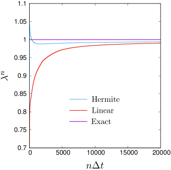
Figure 1 illustrates the results of a typical simulation, starting on the left with the evolution of the estimate of the SCGF, given by (49), as time increases. We observe a very good agreement in the long run with the exact value, which for the parameters used is equal to 1, with a faster convergence observed for the Hermite basis compared to the linear basis. As mentioned before, we can also recover the SCGF by recording the stationary value of $A_{T}$, which corresponds as above to $m_{k}=a_{k}=\lambda^{\prime}(k)$, and numerically integrate the result in $k$ from $\lambda(0)=0$. The results obtained are similar to those obtained from the eigenvalue estimate (49), and are not shown for this reason.

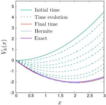
To understand the convergence of the eigenvalue at the process level, we show in the right plot of Fig. 1 the evolution of the effective potential $V_{k}(x)$ associated with the modified drift $b_{k}(x)$ according to

$$b_{k}(x)=-V_{k}^{\prime}(x).$$ (62)

We show the results for both the linear basis and the Hermite basis, with the zero of the potential arbitrarily set at $V_{k}(0)=0$. We see from these that the tail of the potential takes longer to be estimated correctly, as the process starts to explore values away from $m_{0}=0$. After the convergence time, there is a good agreement with the parabola

$$V_{k}(x)=\theta(x-m_{k})^{2},$$ (63)

which is the exact solution predicted by (59). The small errors are due to the finite time step $\Delta t$ used and the finite basis function set. The small “wiggles” seen in the potential obtained with the linear basis come from the fact that this basis is piecewise linear, so that $V_{k}(x)$ is piecewise logarithmic. The potential obtained with the Hermite basis is smoother, as expected.

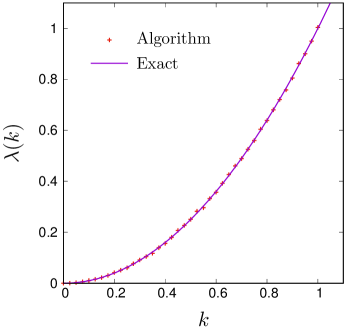
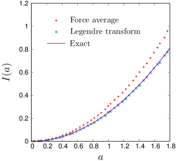
Repeating the simulations for other values of $k$, we can recover $\lambda(k)$, as shown in the left plot of Fig. 2. The result is in good agreement with the exact solution (55). Estimating $\lambda^{\prime}(k)$ with (20) leads to an estimated rate function, by the Legendre transform (25), which also agrees well with the exact rate function, shown in the right plot of Fig. 2. By comparison, the rate function obtained from the time average (24) of the extra biasing force (with the Hermite basis) is not as good: it lies above the exact rate function and shows a larger offset or error as $k$ increases, which does not decrease by reducing $\Delta t$ or increasing the number of basis functions.

Figure 2: Large deviations of the mean area for the Ornstein-Uhlenbeck process. Left: Estimated SCGF compared with the exact result. Right: Estimated rate function based on the Legendre transform of the SCGF and on the averaging of the biasing force (using the Hermite basis), compared with the exact result.

To understand this error, we show in the left plot of Fig. 3 the evolution of the extra biasing force $F_{n}$ for $k=1$, estimated at the current location of the system, which should approach the constant $2$, following (57). The evolution is noisy, as can be seen, which is expected, since $F_{n}$ is estimated by the logarithmic derivative

$$F_{n}(x)=2\frac{(h^{n}(x))^{\prime}}{h^{n}(x)},$$ (64)

computed in the function basis from (46). The derivative amplifies the Monte Carlo errors inherent in the estimate $h^{n}$. In addition, the denominator often takes small values away from the mean position $m_{k}$, which makes the estimation of the optimal force still more difficult. The right plot of Fig. 3 shows that the noise on $F_{n}$ is considerably filtered out by the time average underlying the estimator $R_{T}$ of the rate function, although a bias remains even after the convergence time of the SCGF, which leads to the offset seen in Fig. 2. The results in both cases are more noisy for the linear basis because the derivative is not continuous across the different cells.

Figure 3: Large deviations of the mean area of the Ornstein-Uhlenbeck process. Left: Biasing force $F_{n}$ at the current state $\tilde{x}_{n}$ of the process at time $n$. Right: Evolution of the time average $R_{T}$, which gives the rate function according to (24).

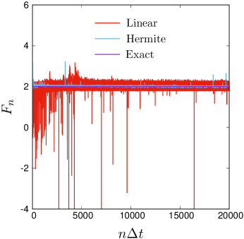
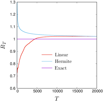
The offset on $R_{T}$ remains more or less constant by running independent simulations (error bars on 30 simulations are too small to show), and so appears to be a systematic error or bias. Many factors can account for this bias. First, the rate function estimated from the limit shown in (24) is known to be an upper bound on the true rate function Chetrite and Touchette (2015b), which is tight if and only if the modified drift estimated in the simulation is the optimal control drift (17). Here, $F_{n}$ is not constant, as predicted from (57), so we expect the estimate $R_{T}$ to lie above its expected value. Second, we have noticed in simulations that $A_{T}$ underestimates $a_{k}$ for large $k$, which has the effect of further “pushing” the estimate of the rate function above $I(a)$. This is most likely due again to $F_{n}$ being non-constant. Finally, the time average of $F_{n}$ involves the ratio of two functions, according to (64), which fluctuate in time via the updating of $\alpha^{n}$ in (46). As a result, we expect this additional randomness to artificially increase the second moment of $F_{n}$, leading to a further bias.

It is difficult to isolate these factors, and all, in fact, seem to play a role. In future works, it would be interesting to study the bias observed in $R_{T}$ by computing, for example, the time average of $F_{n}^{2}$ using the final estimate of $h_{k}$ rather than the time-evolved estimate $h^{n}$. Different annealing sequences or averaging techniques could also be used to “filter” the time average of $F_{n}^{2}$ and mitigate the bias on $R_{T}$. For now, the most efficient and reliable way to compute the rate function is to use the estimator based on the SCGF and its Legendre transform.

IV.2 Periodic diffusion

We consider for the second test a diffusion on the unit circle satisfying the SDE

$$dX_{t}=(-V^{\prime}(X_{t})+\gamma)dt+\sqrt{2}\,dW_{t},$$ (65)

with the periodic potential $V(x)=\cos(2\pi x)$ and $\gamma\in\mathbb{R}$ a constant drive. For $\gamma\neq 0$, the total drift cannot be expressed as the gradient of a smooth periodic function, so $X_{t}$ is a nonequilibrium process violating detailed balance Risken (1996). The observable studied for this process is the winding number

$$A_{T}=\frac{1}{T}\int_{0}^{T}dX_{t},$$ (66)

calculated with the real rather than periodic state, which can be interpreted physically as the mean velocity or current of a Brownian particle moving around the circle Tsobgni Nyawo and Touchette (2016). In the notation of Sec. II, we have $b(x)=-V^{\prime}(x)+\gamma$, $\sigma=\sqrt{2}$, $f(x)=0$, and $g(x)=1$.

The SCGF and the rate function of this observable are not known exactly, but Galerkin approximations can easily be found by Fourier series, using the basis functions $\phi_{j}(x)=\mathrm{e}^{j2\pi\mathrm{i}x}$ with $j\in\mathbb{Z}$ Mehl et al. (2008); Nemoto and Sasa (2011); Tsobgni Nyawo and Touchette (2016). This basis is used to compute reference values for the SCGF and the rate function, devoid of $\Delta t$ errors, by projecting the spectral problem (14) in Fourier space and by ensuring that enough basis functions are used. We find in practice that $M=41$ Fourier modes are sufficient. We use the same Fourier basis for the algorithm, also with $M=41$ modes, in addition to $T=2\times 10^{4}$ and $T_{1}=T_{2}=2\times 10^{3}$ for the integration times, as in the first test.

Figure 4: Current large deviations of the driven periodic diffusion. Left: Evolution of the estimated SCGF with time for different time steps $\Delta t$. Right: Estimated eigenfunction $h_{k}$ for different time steps $\Delta t$ compared with the reference Fourier solution.

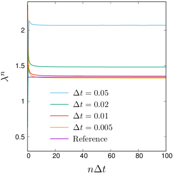
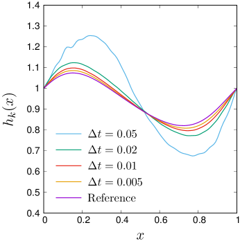
We show in Fig. 4 the results of a typical simulation for $\gamma=1$ and $k=1$. The left plot in this figure shows the evolution in time of the estimated SCGF from the eigenvalue iteration (49), while the right plot shows the final estimated eigenfunction $h_{k}$ for different time steps $\Delta t$, compared with the reference Fourier solution. We see that the results for the eigenvalue and the eigenvector significantly depart from the reference solutions for $\Delta t=0.05$, but converge to them as $\Delta t$ is decreased, in accordance with Assumption 2 and the theoretical results of Ferré and Stoltz (2017). For the same time step used for the Ornstein-Uhlenbeck process, namely, $\Delta t=5\times 10^{-3}$, we see no notable difference between the estimated eigenfunction and the reference values, leading to a precise estimation of the SCGF. The convergence of the eigenvalue here is much faster than for the Ornstein-Uhlenbeck process because the space explored is compact, being limited to $[0,1]$ with periodic boundary conditions.

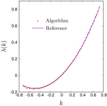
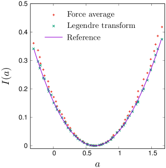
As for the Ornstein-Uhlenbeck process, we can repeat these simulations over a range of values for $k$ to obtain the SCGF and the rate function. The left plot of Fig. 5 shows that the SCGF is in good agreement with the Fourier solution for $\Delta t=5\times 10^{-3}$, and so is the rate function estimated by Legendre transform. However, as seen before, the rate function estimated with the time average $R_{T}$ of the biasing force shows an offset, although smaller this time, which comes from the noisy estimation of $F_{n}$. As before, the estimator of the rate function that should be used is the one based on the Legendre transform of the SCGF, with $a_{k}$ estimated by $A_{T}$.

Figure 5: Current large deviations for the driven periodic diffusion. Left: Estimated SCGF compared with the reference Fourier solution. Right: Estimated rate function based on the Legendre transform and on the averaging of the biasing force, compared with the reference Fourier solution.

V Conclusion

We have presented a new algorithm for estimating the large deviation functions of time-integrated observables of Markov processes, which characterize the likelihood of their fluctuations in the long-time limit. The algorithm draws on earlier results on stochastic control Borkar et al. (2004); Ahamed et al. (2006); Basu et al. (2008); Borkar (2010), and works by adaptively estimating the principal eigenvalue and eigenfunction of a spectral problem related to the large deviation problem. The adaptive part consists in modifying the process considered, using feedback and reinforcement learning, so as to reach the so-called driven process, which is known to be optimal for the purpose of estimating large deviation functions using importance sampling Chetrite and Touchette (2015b). In this sense, the algorithm relates to many adaptive importance sampling methods that have been proposed recently for rare event simulations; see, for instance, Dupuis and Wang (2005); Nemoto et al. (2017b); Blanchet and Lam (2012); Kappen and Ruiz (2016). It is also closely related to diffusion Monte Carlo methods Foulkes et al. (2001); Rousset (2006); Lim and Weare (2017), which attempt to estimate the ground-state wavefunction of a many-body quantum system by simulating a related stochastic process.

The proposed algorithm can be applied to diffusions, as illustrated here, but also to Markov chains in discrete or continuous time, and works for both equilibrium and nonequilibrium systems, that is, reversible and non-reversible processes, respectively. Moreover, although the test cases that we have presented are simple, they clearly show that the algorithm has the potential to improve upon other simulation methods, especially cloning methods, since it runs on a single simulation of the process and provides information about how fluctuations are created in time by constructing the driven process in a non-parametric form and with no prior information. A modification of the original cloning algorithm was proposed recently Nemoto et al. (2016) to construct the driven process, but it is based on a different feedback rule that compares two time-dependent histograms, whose estimation is noisy and requires a large number of clones. The results presented here show that a single clone, evolving over a long-enough time, is sufficient. This obviously cuts the computational complexity of estimating large deviations, but also simplifies, as mentioned, the error and convergence analyses of the algorithm.

As with any new proposal, more work is needed to understand the benefits and limitations of the algorithm, to test its applicability to realistic systems, and to benchmark it against other numerical methods. Of particular importance is to derive precise error estimates associated with the space and time discretizations of the spectral elements, large deviation functions, and the driven process. Recent results about the discretization errors in $\Delta t$ for the SCGF can be found in Ferré and Stoltz (2017). These discretization errors are also present in cloning algorithms when applied to diffusions, so they are not specific to the algorithm presented here. The use of Galerkin discretizations is also common to both algorithms and requires further investigations, particularly in the low-noise limit and for processes involving many interacting particles.