Isospectral domains for discrete elliptic operators111 This work has been partially supported by GNCS-INDAM (Gruppo Nazionale Calcolo Scientifico - Istituto Nazionale di Alta Matematica).
Abstract
Concerning the Laplace operator with homogeneous Dirichlet boundary conditions, the classical notion of isospectrality assumes that two domains are related when they give rise to the same spectrum. In two dimensions, non isometric, isospectral domains exist. It is not known however if all the eigenvalues relative to a specific domain can be preserved under suitable continuous deformation of its geometry. We show that this is possible when the 2D Laplacian is replaced by a finite dimensional version and the geometry is modified by respecting certain constraints. The analysis is carried out in a very small finite dimensional space, but it can be extended to more accurate finite-dimensional representations of the 2D Laplacian, with an increase of computational complexity. The aim of this paper is to introduce the preliminary steps in view of more serious generalizations.
1Dipartimento di Matematica e Informatica
Università di Camerino, Via Madonna delle Carceri 9, 62032 Camerino (Italy)
2Dipartimento di Fisica, Informatica e Matematica
Università di Modena e Reggio Emilia, Via Campi 213/B, 41125 Modena (Italy)
1 Introduction
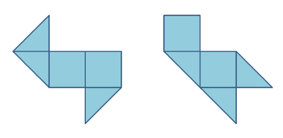
Consider the Laplace problem in 2D with homogeneous Dirichlet boundary conditions defined in an open set with regular boundary (see [6] for a general overview). It is known that there are distinct domains (non isometric) such that all the infinite eigenvalues of the Laplace operator coincide (see, e.g., Fig. 1). For this reason, these are called isospectral domains. It can be shown that two isospectral domains have the same area. It is not known however if it is possible to connect with continuity two isospectral domains through a sequence of domains, by preserving the whole spectrum.
Partial answers can be given by working in a finite dimensional environment. Here, we take a suitable approximation of the Laplace operator corresponding to a negative-definite matrix. By varying the domain, we are interested to detect those deformations that preserve the entire set of eigenvalues (that are now in finite number). At the same time, not all the possible deformations are allowed, but only those belonging to a finite dimensional space of parameters. The problem turns out to be far from easy. Indeed, already at dimension 4, things get rather involved. The question examined here concerns with the deformation of quadrilateral domains, with the aim of preserving the eigenvalues of discrete operators obtained from collocation of the Laplace problem using polynomials of degree 3 in each variable. By imposing Dirichlet homogeneous boundary conditions, the discretization matrix ends up to be only of dimension . The vertices of the domains are then suitably moved by maintaining the magnitude of the four corresponding eigenvalues. The results show that, at least in these simplified circumstances, families of isospectral domains exist and can be connected by continuous transformations.
The most straightforward (but extremely expensive) approach is to try all the possible allowed configurations and sort them by comparing the so obtained spectrum. Upgraded versions consist in moving the vertices along curves, whose tangent is obtained as an application of the Implicit Function theorem due to U. Dini (see, for example, [8]). Here, one computes with the help of symbolic manipulation the partial derivatives, with respect to the various parameters, of the coefficients of the characteristic polynomial of the matrix representing the discrete operator. Different, more or less efficient, approaches have been tested. By the way, despite its simple formulation, the problem looks rather complex and the extension to higher dimensions or to more complicated domains looks at the moment quite unrealistic.
2 Preliminary settings
For the convenience of the reader we briefly review some results about the classical eigenvalue problem for the Laplace operator: , in an open set , when homogeneous Dirichlet boundary conditions are imposed on the boundary . The problem is formulated as follows:
| (1) | |||||
| (2) |
It is known (see, e.g.: [6]) that the spectrum of minus the Laplace operator is discrete, that the eigenvalues are non negative and can be ordered in ascending order to form a divergent sequence:
| (3) |
with possible multiplicities. When the eigenvalues are:
| (4) |
The Weyl’s law establishes an estimate of the -th eigenvalue in terms of the area of the domain where the eigenvalue problem is defined:
| (5) |
This relation leads us to the following consequence. For a given , one denotes by the number of eigenvalues smaller than . Then, a Weyl’s theorem states that:
| (6) |
It turns out that, if two distinct domains produce the same set of eigenvalues (i.e., they are isospectral), they must have the same area. A refinement of property (6) brings to the relation:
| (7) |
known as Weyl’s conjecture, which also involves the length of the perimeter , i.e. . This means that, provided the conjecture is verified, isospectral domains also share the same perimeter.
The existence of (non isometric) isospectral domains has been established quite recently. The problem was firstly formulated in [7], where the author was wondering if the eigenspectrum of the Laplacian was sufficient to detect the shape of the domain (put in other words: if one can hear the shape of a drum). In the 2D plane, the negative answer appeared in [5], where distinct domains (see, for example, Fig. 1) exhibiting identical sets of eigenvalues, were proposed. Preliminary results in this direction were investigated in [9]. Successive examples have been discussed for instance in [1] and [2]. Nowadays, wide classes of isospectral domains are available. For the sake of brevity, we address the reader to the specialized literature for more insight.
Some facts are still not known however, as for instance the existence of 2D isospectral domains of convex type, or the possibility to vary with continuity the shape of a given domain maintaining at the same time its entire spectrum. This last property is the one we are going to investigate in this paper, when the Laplace operator is substituted by a very rough finite-dimensional version. In fact, in this paper we want to see if, under suitable simplified hypotheses, it is possible to connect with continuity two isospectral domains through a sequence of domains, by preserving the whole spectrum.
Our first goal is to define a general set of quadrilateral domains. Afterwords, starting from a given member of the family, we will try to find other members that are isospectral to it. The notion of isospectrality is decided according to a finite-dimensional elliptic operator that is going to be introduced in Sect. 3. First of all, we need to exclude as much as possible, the chance of having isometric domains in the family, i.e, quadrilaterals that can be related through elementary operations, such as translation, rotation and symmetry. Of course, two isometric domains are automatically isospectral and we would like to avoid such trivial connections.
 (a)
(a) 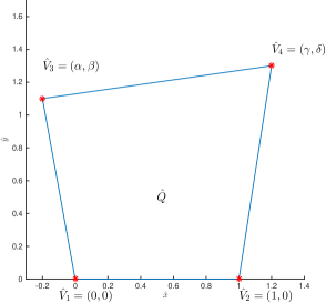 (b)
(b)
From now on we assume that one of the sides of our quadrilaterals is “nailed” to the -axis of the plane. Moreover in the future, we shall avoid those cases in which a couple of sides may intersect at some internal point.
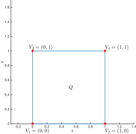
Let be a positive integer, be the set of real numbers, be the -dimensional real Euclidean space. Let be the unit square in the space , i.e., is the quadrilateral of vertices , , , (see Fig. 2). Given the real parameters , let be the generic quadrilateral of our family, having vertices , , , (see again Fig. 2). The domains and are open.
In the plane with coordinates , we now focus our attention on the eigenvalue problem for the Laplace operator defined in , with homogeneous Dirichlet boundary conditions on the piecewise smooth boundary . Translating into formulas, we have:
| (8) | |||||
| (9) |
where .
For convenience, let us map problem (8), (9) into the following modified version, defined in the square :
| (10) | |||||
| (11) |
where turns out to be a suitable positive-definite elliptic operator that we are going to define here below. To this scope let us examine the transformation , that allows us to bring the operator into . First of all let us transform a general quadrilateral into the reference square . We use a classical invertible mapping consisting of polynomials of degree one in each variable. This relates the ordered points , , , of with the ordered points , , , of (see Fig. 2). The two components of the transformation are given by:
| (12) | |||
| (13) |
Thus, a function defined in is associated with the function defined in . By applying the change of variables to the Laplace operator we arrive at the eigenvalue problem (10), (11) where the operator is defined as follows (see [4]):
| (14) |
and the coefficients of in (14) are given by:
| (15) | |||
where
| (16) |
is the determinant of the Jacobian of .
In the future, instead of solving the eigenvalue problem directly on , we will find more convenient to approach the transformed eigenvalue problem defined in . That is, instead of approaching problem (8), (9) we consider problem (10), (11) where is defined in (14). It is straightforward to check that when .
As explained with more details in Sect. 4, it is also convenient to introduce a new parameter . Through the homothety centered at the origin , we associate a generic point of the plane to the point . In this way, any given eigenvalue of in the domain takes the form in the new domain . By this trick, without too much effort, we can enlarge the set of quadrilaterals at our disposition.
3 The discrete operator
In the referring domain we now build a discrete elliptic operator corresponding to a very rough approximation of the operator defined in (14). Indeed, we do not want to handle too many eigenvalues. The reason is that the family of quadrilateral domains introduced in the previous section only depends on five degrees of freedom (that is , , , , ). Therefore, the isospectrality will be judged on the basis of very few eigenvalues. Our discretized operators correspond to matrices, so that we can only account on four eigenvalues. This is the maximum number that allows us to find continuously connected subfamilies of isospectral domains. In fact, having more eigenvalues to handle can lead to an unsolvable problem, since we do not have enough parameters to deform the domains. Thus, we will look for a curve in the five-dimensional space, in such a way four nonlinear equations (expressing the coincidence of the eigenvalues in relation to an initial given quadrilateral) have to be simultaneously satisfied.
A first basic approach consists in implementing the classical finite difference method to approximate the operator defined (14) and related to the eigenvalue problem (10), (11). We recall that, when the quadrilateral coincides with the square , one has , and the corresponding eigenvalue problem is given by (1), (2).
We take a uniform grid with step size in the unit square , both in the and directions. In particular, we divide the interval into three equal subintervals of length . The corresponding grid points are defined by:
| (17) |
Let , , , be the internal points of the grid .
In these circumstances using centered finite differences and taking into account the vanishing Dirichlet boundary condition on the boundary of (see (11)), we have that the differential operators , , , and , can be, respectively, approximated with the discrete operators , , , and given by the following matrices:
| (18) |
Finally, given the functions , in (2) and defined the five matrices:
| (19) |
we have that the finite differences operator approximating the differential operator on the grid can be written as follows:
| (20) |
where denotes the usual matrix multiplication. In this way the discrete eigenvalue problem associated to problem (10), (11) can be written as:
| (21) |
where the eigenvector belongs to .
Better discretizations of and are obtained by spectral collocation. In this simple circumstance one can use polynomials of degree three in each variable. They must satisfy the vanishing constraint on the boundary of , so that one easily checks that the dimension of the approximating space is reduced to four degrees of freedom. Thus, we collocate equation (10) at the four inner grid points in order to close the system.
Indeed, we can also generalize the grid by introducing a new parameter , with , and by considering the following set of points in the unit square :
| (22) |
where
| (23) |
Of course, the internal nodes are: , , , . They correspond to the classical uniform grid when . Another suitable choice is to set . In this way the values and are the zeros of the first derivative of the Legendre polynomial .
Let us now consider a generic polynomial of degree 3 in each of the two variables and :
| (24) |
for some coefficients , . In (24) , are the one-dimensional Lagrange polynomials of degree 3 with respect to the nodes: . In particular and vanish at the endpoints, and we have:
| (25) |
By calculating explicitly the derivative of and collocating at the grid points in (22), one obtains the matrices: , , , and , approximating, respectively, the differential operators , , , and .
Finally, as in (20), a spectral discretization of the operator in the domain takes the form:
| (26) |
where the matrices , are defined in (19). This leads us to the eigenvalue problem:
| (27) |
where the eigenvector belongs to .
We now discuss some practical cases. Suppose that , i.e., we are dealing with problem (1), (2). From (4) we have that the first four exact eigenvalues of minus the Laplace operator in the square are: . Regarding the discretization of by finite differences we find: . These values coincide with those of the spectral approximation for . By using the spectral approximation with we obtain instead .
4 First attempts
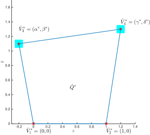
Given the family of quadrilateral domains of vertices , , , , we begin our study by fixing an initial quadrilateral of vertices , , , with (see Fig. 3). From now on the superscript is used to point out that the domain has been fixed, and we would like to examine what happens in its neighborhood in terms of isospectrality.
As shown in Sect. 3, the quadrilateral is mapped to the referring square producing the new operator . By using the finite difference approximation (20) or spectral collocation as in (26), the discrete operator can be either represented by the matrix or by . Correspondingly, problems (21) or (27) must be solved.
From now on, we only work with with and, by solving (27), we find four positive eigenvalues, that will be denoted by . For example, as anticipated in the previous section, by taking the quadrilateral of vertices
| (28) |
shown in Fig. 2 (see also Fig. 3) and solving (27) with , we obtain the following outcome:
| (29) |
 (a)
(a) 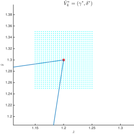 (b)
(b)
Our goal is to see if there exist other quadrilaterals leading to the same set of eigenvalues and if these can be connected by a curve. The reason why we did not start our analysis with the unit square and its isospectral companions will be clarified later on in Sect. 7.
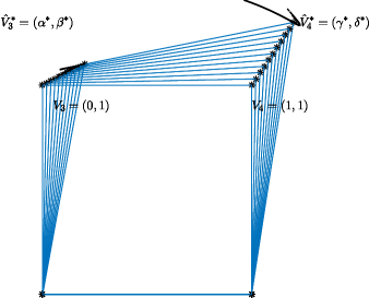
Since we do not have at the moment any theoretical result, a rough way to have an idea of what happens it to check methodically a great number of quadrilaterals in the neighborhood of the initial one. To this purpose, we construct two little squares with sides of length centered at the points and as shown in Fig. 3. After defining appropriate grids of given size in these two squares, we try all the possible combinations. For each couple of grid-points (one in the first square and one in the second square) we have a quadrilateral (recall that and have been fixed). From this we deduce a matrix, and finally four eigenvalues. We call the set of all quadrilaterals obtained in this fashion: -range.
We then select those configurations in the -range displaying the same eigenvalues given in (29), up to a prescribed error . We can call these special domains -isospectral. The sizes of and have to be set up with the aim of finding reasonable outcomes. In fact, if is too large we may end up with too many -isospectral domains; otherwise for too small we could discover that the only acceptable domain is the starting one . Similar situations could also occur by selecting inappropriately. The procedure is quite costly, especially for small and . This is the reason why in the next sections we look for something more convenient from the numerical viewpoint.
Unfortunately, the results of this analysis are not encouraging. Indeed, it seems that there are no enough degrees of freedom to play with, and this is the reason why in Sect. 2 we introduced the new parameter . This is an amplification (or reduction) factor that allows us to include in the set of possible -isospectral candidates other quadrilaterals. These are obtainable through a suitable homothety centered in . Through this homothety we associate a generic point of the plane to the point . In this way, any given eigenvalue of relative to a generic domain takes the form in the new domain . By this trick, without too much effort, we can enlarge the set of quadrilaterals at our disposition.
Thus, we argue as follows. For a given domain in the -range, we will also accept eigenvalues that are proportional to those in (29) through a multiplicative constant depending on . To this end we set . Afterwards the domains are going to be selected according to the formula:
| (30) |
If the above inequality is satisfied for , the corresponding quadrilateral is directly -isospectral to the starting one. If , then the actual -isospectral quadrilateral is obtained by multiplying the coordinates by the constant .
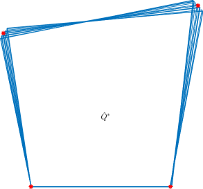
For example, starting from the quadrilateral in (28) shown in Fig. 3 (which eigenvalues are listed in (29)), we adopted the above procedure based on the parameters: , and . A family of 47 -isospectral domains in the -range was obtained. Some of these are displayed in Fig. 4. Concerning the operator in (20), preliminary results of this type were found in [3].
We checked areas and perimeters of the 47 -isospectral domains. Within a tolerance of , 46 out of 47 quadrilaterals (including ) share the same area, and 29 have the same perimeter. Note that, in our discrete case, we cannot rely on a result similar to that of Weyl for the continuous case. Nevertheless, the discovery that areas are (almost) preserved, besides being in agreement with predictions, is an excellent tool to decide a priori if a domain is appropriate. Indeed, before directly computing the eigenvalues, one can filter those domains that, up to a certain accuracy, share with the initial one the same area. This preliminary control saves a lot of computational time.
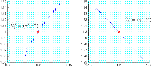
Note that the vertex remains fixed, while the vertex shifts horizontally. This means that, except for the initial configuration where the parameter is equal to one, the values of are in general different from one. The plots in Fig. 5 are the zooms of the two little squares with sides of length of Fig. 3 centered at the points and . From these images we can conjecture the existence of a continuous path joining the various -isospectral domains. Although only based on heuristic considerations, the guess seems to be confirmed by further tests, where and are conveniently taken smaller and smaller. We can be more precise in the coming sections, where appropriate strategies will be developed to prove the existence of these curves and detect them.
Similar results are obtained by varying the configuration of the initial quadrilateral . We suggest however to set the initial parameters in order to stay away from some critical situations that will be analyzed more in detail in Sect. 7.
5 Implementation of the Implicit Function theorem
From the experiments of the previous section, our guess is that a curve joining isospectral quadrilaterals actually exists. It is a one-parameter function embedded in the 5 dimensional space spanned by the parameters , , , , . We can track it by observing that it is implicitly characterized through four functional equations. We can follow the curve by computing locally its tangent vector and this can be done with the help of the Implicit Function theorem (see, for example, [8]). Actually, in circumstances in which such a theorem is applicable, we automatically have an existence result, at least at local level.
We recall that a generic quadrilateral has vertices of the form , , , . Afterwords, for let be the eigenvalues in ascending order of the discrete problem (27). Clearly, each one of these quantities depends on the parameters , i.e.:
| (31) |
Now, the eigenvalues (31) can be seen as the roots of the following characteristic polynomial:
| (32) |
where the coefficients , , are computed from the entries of the matrix defined in (26). As a consequence these coefficients also depend on , that is , .
As done in the previous section, we can work around an initial domain of fixed vertices , , , with . For instance, we can start from the quadrilateral specified in (28) and shown in Fig. 3, whose corresponding eigenvalues are listed in (29). Accordingly, , are the roots of the following characteristic polynomial:
| (33) |
where now the coefficients , , are given real numbers. For example, starting from the quadrilateral in (28), we have:
| (34) |
Thus, a certain quadrilateral (with vertices , , , ) is isospectral to if and only if and have the same roots, i.e., one has , . We can weaken this condition by introducing the parameter . Indeed, we can also accept situations where the eigenvalues are proportionally related as follows:
| (35) |
If , turns out to be directly isospectral to . If , the new domain , obtained by homothety, is also isospectral to (note that in this case the second vertex becomes ). We can now translate condition (35) in terms of polynomial coefficients, obtaining:
| (36) |
In the end, we propose to introduce the four functions , of the five variables , defined as follows:
| (37) |
and look for values such that:
| (38) |
If we are lucky, there is a local curve , , , described by the functions , , , , , passing through the point of coordinates , , , , (i.e., the parameters identifying the initial quadrilateral as in (28)) and connecting isospectral domains.
In order to follow such a curve , we need to find its local tangent vector. We can express the various parameters in function of one of them. We fix for example , with , so that . We then differentiate with respect to the four equations in (38), arriving at the system:
| (39) |
in the unknowns , , and .
At this point, it is important to observe that the functions , , in (37) and their derivatives are explicitly known, although their expressions may result rather complicated. In fact, starting from , , , , one can build the coefficients of the mapping into the referring square. Successively, always in function of these parameters, one writes the matrix defined in (26). Finally, a closed form is also known for the coefficients of the characteristic polynomial (this is not true instead for the eigenvalues). Of course, from the practical viewpoint, these computations can only be carried out with the help of a software running with symbolic manipulation.
Going through this calculation, we find that the determinant of the matrix in (39) is different from zero at . Therefore, one is able to theoretically detect a value , such that a curve , , described by the parameters , , , , , actually exists in the interval . For , we have .
The following first-order explicit iteration method can be adopted in order to follow the curve, at least locally. Recall that, given , we have chosen , . For simplicity let us fix our attention on positive value of the variable (indeed similar arguments may also be applied when is negative) and, given an integer , let us discretize the interval with a uniform grid , , with step size , that is:
| (40) |
Our curve is going to be approximated by the quantities , . In particular . At each step, the exact derivatives , , and , , are computed by solving (39) (note that , ). These exact derivatives are organized in the correcting vector , . The algorithm is then based on the following iteration:
| (41) |
A similar procedure can be used to approximate the curve in the interval .
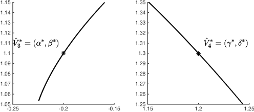
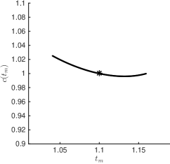
For example, we discuss the case of the quadrilateral in (28) shown in Fig. 3 and we take , . We apply (41) with , both for positive and negative values of . Fig. 6 and Fig. 7 show, respectively, the projections of , , in the planes , and the graph , . These results confirm what was predicted in the previous section.
As expected, the shapes of the projections of the curve turn out to be exactly the same if, instead of the parameter , another parameter is assumed to be explicit.
6 Other approaches
The use of symbolic manipulation, in order to compute the exact tangent vector to the curve at a given point, is certainly expensive, ill-conditioned and difficult to be generalized. It has been however an important theoretical tool to establish the local existence of the curve. In this section we propose an alternative numerical procedure, far more cheaper but with similar performances.
In line with the arguments invoked in Sect. 5 and using the same notation we have that, if the curve has to connect isospectral domains, the eigenvalues , , in (35) must remain the same as varies. In particular we have: , . That is, having in mind (31), the four functions , of the five variables , defined as follows:
| (42) |
must be constant, i.e., their derivatives with respect to are zero. By differentiating (42) with respect to and by expressing the various parameters in function of one of them, we find the approximated local tangent vector to the curve .
As in Sect. 5 let us fix for example , with , so that . The new linear system takes the form:
| (43) |
in the unknowns , , and .
Since now the explicit expression of the partial derivatives in (43) is not available, the entries of the matrix are approximated by classical finite differences, that is, for example, given an increment , we can compute , , as follows:
| (44) |
Similar formulae can be used to approximate the other entries of the matrix in (43).
Finally, we use the uniform grid (40) when is positive (or its opposite when is negative). At step , we evaluate the approximations of , , and , (note that , ), by solving a system similar to that in (43), where partial derivatives have been replaced with incremental ratios. We put the so obtained values in the current vector , . Thus, a rough approximation of is given by the quantities , , recovered by recursion from the following explicit iteration method:
| (45) |
starting from .
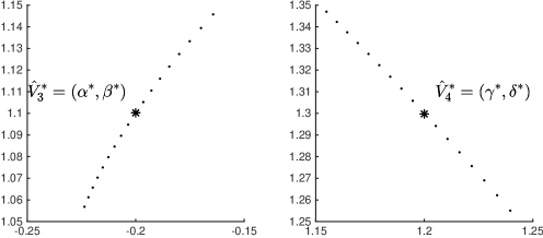
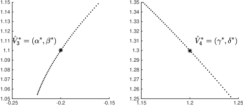
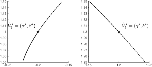
Given the quadrilateral corresponding to (28) and shown in Fig. 3, by taking , , we apply the iteration method (45), both for positive and negative values of . Different values of the step size are used. In particular we choose . In Fig. 8 we show the projections of , , in the planes , . As diminishes, the graphs of Fig. 8 approach those of Fig. 6.
Also in this case the shape of the projections of the curve turn out to be qualitatively the same if another parameter is assumed to be explicit (instead of the parameter ).
This convergence behavior is a good surprise. Indeed, such a property should not be given for granted. In fact, through (44) and similar formulae, we replaced partial derivatives by a first-order approximation, and we introduced this correction in the first-order algorithm (41). This double discretization does not necessarily bring to a convergent scheme.
 (a)
(a)
 (b)
(b)
 (c)
(c)
A sort of convergence analysis can be carried out by examining the history of the quadrilateral areas in comparison to the area of , given by . The results of some tests are reported in Table 1. For a fixed the error grows linearly with the distance from the quadrilateral . Nevertheless, there is no substantial decay of the error by diminishing . It has also to be noted however that, in the discrete case, we do not have any theoretical result ensuring that areas of isospectral domains must be preserved.
We finally observe that the results obtained so far do not change significantly if other values of the parameter introduced in (23) are taken into account (we recall that in the experiments reported in this paper we used ).
| and =0.012 | and =0.006 | and =0.003 | |
| 1.040 | 11.70 e-04 | 10.30 e-04 | 9.65 e-04 |
| 1.052 | 9.91 e-04 | 8.69 e-04 | 8.12 e-04 |
| 1.064 | 7.83 e-04 | 6.84 e-04 | 6.37 e-04 |
| 1.076 | 5.48 e-04 | 4.76 e-04 | 4.43 e-04 |
| 1.088 | 2.87 e-04 | 2.48 e-04 | 2.30 e-04 |
| 1.1 | 0 | 0 | 0 |
| 1.112 | 1.53 e-04 | 1.89 e-04 | 2.07 e-04 |
| 1.124 | 3.09 e-04 | 3.85 e-04 | 4.25 e-04 |
| 1.136 | 4.67 e-04 | 5.89 e-04 | 6.54 e-04 |
| 1.148 | 6.26 e-04 | 8.00 e-04 | 8.92 e-04 |
| 1.160 | 7.86 e-04 | 10.19 e-04 | 11.42 e-04 |
7 The case of the square
Here, we discuss about the case of the unit square , i.e. the quadrilateral of vertices , , , , and the case of other domains of vertices , , , that are symmetric with respect to the straight line , that is domains with , and . Of course, when , , we have .
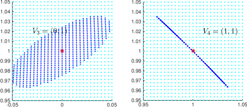
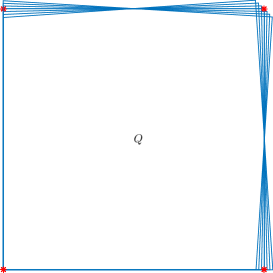
In these situations using the approach proposed in Sect. 5, one can check that the determinant of the matrix in (39) is always zero. We remind that in Sect. 5 we have chosen , , but, indeed, the determinant remains zero independently on the explicited parameter. Moreover, for the square , the rank of the matrix in (39) is just one, i.e. all the lines (or rows) of the matrix are linearly dependent. Definitely, we are not in the situation that allows us to use the Implicit Function theorem. Nevertheless, experimentally, one can find in the neighborhood of the unit square many other quadrilaterals isospectral to it. An analysis similar to that of Sect. 4 reveals configurations as the ones shown in Fig. 9. In this case we choose: , and , and, as in Sect. 4, we considered . In the neighborhood of the vertex on the left of Fig. 9 the distribution of selected points does not reveal specific patterns, while for the vertex on the right of Fig. 9 there is a superimposition of several curves, as it will be evident from the discussion that follows.
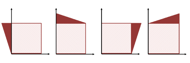
A heuristic explanation of the non applicability of the Implicit Function theorem is inspired by Fig. 10, where the four parameters , , , , are varied independently (one has to imagine that these deformations are infinitesimal). One gets four configurations corresponding to quadrilaterals that are reciprocally isometric (by rotations or symmetries), and therefore isospectral. This somehow explains why the Jacobian matrix in (39) has rank equal to one. Analogous conclusions hold for other initial domains presenting symmetries.
 (a)
(a) 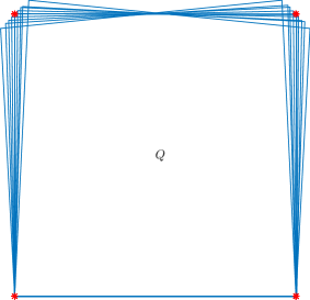 (b)
(b)
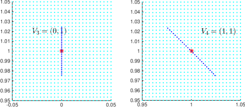
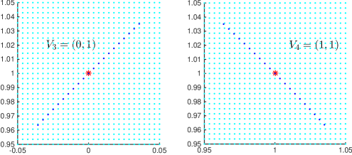
The above considerations do not prevent however the existence of curves connecting isospectral domains. Actually, in correspondence of the parameters associated with the unit square we have a biforcation point. A deeper study shows that different curves of isospectral quadrilaterals are obtained. For instance, we can have those of the family associated either with the points of Fig. 12 or with the points of Fig. 12. In particular, Fig. 13 shows the quadrilaterals corresponding to the two ways of deforming the square . These two branches of isospectral domains departing from the unit square are very neat. Nevertheless, their identification is not easy if one only examines Fig. 9. Of course, when we started our analysis we (erroneously) thought that the case of the square was the easiest one; only later we realized that this was far from being true.
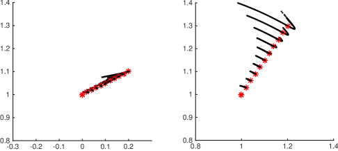
We conclude this section with a few more experiments. We would like to figure out what happens to the curve connecting isospectral domains when the initial quadrilateral is modified. For example, we can start from the quadrilateral associated with the vertices in (28). The corresponding isospectral family forms a curve characterized by the projections shown in Fig. 6 (also reported in Fig. 15). Now, we deform such initial domain by slowly approaching the unit square . To this purpose, we fix an integer . For , the vertices of the transitory quadrilaterals are chosen according to the law:
| (46) |
In this way, for in (7) we have the initial quadrilateral , i.e. , while for we obtain the unit square , i.e. .
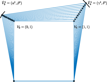
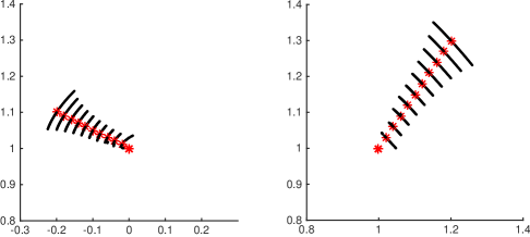
Since we know that, in correspondence of the unit square , the determinant of the Jacobian in (39) is zero, the use of the Implicit Function theorem becomes more and more restrictive as increases. For this reason we need to limit the range of definition of the curve. Given we propose to control this range by defining the extremes , , of the interval according to the rule:
| (47) |
We excluded the value in (47) because in this case the procedure is not applicable.
Starting from the quadrilateral in (28), taking in (7) and in (47), we obtain the various quadrilaterals displayed in Fig. 15. For , we locally compute the curve of the isospectral domains related to , indifferently with the approach proposed in Sect. 6 or Sect. 7. The projections of these curves in the planes and are shown in Fig. 15.
Finally, we run the same tests by using a different set of vertices , , of the initial quadrilateral , namely:
| (48) |
In Fig. 17 and Fig. 17 the reader can see the results of the tests obtained by taking in (7) and in (47). Here the curve is twisting in a more complicated fashion. Scattered dots may appear in the plots. They are a consequence of the break down of the algorithm when approaching the unit square . In order to get rid of them it is necessary to further reduce the interval , as gets close to .
8 Conclusions
Still remaining in finite dimension, the extension of our analysis to general domains depending on more degrees of freedom can be a severe numerical task. The main difficulty is how to choose the family of admissible domains. They may have, for instance, a polygonal boundary and the approximation of the continuous operator can be performed by finite elements. If we are far from special symmetric configurations (as the case of the unit square considered in Sect. 7), the local application of the Implicit Function theorem should guarantee isospectral deformations in a small neighborhood. The one-dimensional curve now belongs to a space of larger dimension and its grafical representation can be rather troublesome. For visualization, the best way is probably to show animations concerning the movement of the isospectral domains. Note that the costs of implementation can drastically become high when increasing the degrees of freedom.
An alternative to the work presented here is to try to preserve a certain number of eigenvalues of the exact operator. For example, concerning the family of quadrilaterals (as those examined so far), instead of introducing a discretization based on matrices of dimension , one can evaluate the first 4 eigenvalues of the exact Laplacian and move the domains with the aim of preserving their values. We expect the so obtained domains to be slightly different from the ones we found in this paper. Unfortunately, the exact eigenvalues of on a general quadrilateral domain are not explicitly available, so that the computation should be accompanied by an appropriate discretization on a very fine grid. Again, the complexity of the algorithm may become unaffordable as more degrees of freedom are introduced.
The problem of finding isospectral families, connected with continuity, in order to preserve all the eigenvalues of the exact Laplace operator is certainly harder than the experiments we tried in this paper, and represents a stimulating theoretical challenge. We hope however that our little contribution may be the starting point for future ideas.
References
- [1] P. Buser, J. Conway, P. Doyle, K.-D. Semmler, Some planar isospectral domains, Int. Math. Res. Not. 9, pp. 391-400 (1994).
- [2] S. J. Chapman, Drums that sound the same, Am. Math. Monthly 102, pp. 124-138 (1995).
- [3] A. Codeluppi, Quadrilateri isospettrali per un operatore in dimensione finita, Thesis, Università di Modena e Reggio Emilia (2013).
- [4] D. Funaro, Spectral Elements for Transport-Dominated Equations, Lecture Notes In Computational Science and Engineering, Volume 1, Springer-Verlag, New York (1997).
- [5] C. Gordon, D. Webb, S. Wolpert, Isospectral plane domains and surfaces via Riemannian orbifolds, Inv. Math., 110 (1), pp. 11-22 (1993).
- [6] D. S. Grebenkov, B.-T. Nguyen, Geometrical structure of Laplacian eigenfuncions, SIAM Rev., 55 (4), pp. 601-667 (2013).
- [7] M. Kac, Can one hear the shape of a drum?, Am. Math. Monthly, 73, pp. 1-23 (1966).
- [8] W. Rudin, Principles of Mathematical Analysis, McGraw-Hill, New York (1976).
- [9] T. Sunada, Riemannian coverings and isospectral manifolds, Ann. Math., 121, pp. 169-186 (1985).