March, 2018

TIT/HEP-664

Worldsheet Instanton Corrections to Five-branes and Waves in Double Field Theory

Tetsuji Kimura${}^{\text{,}}$, Shin Sasaki and Kenta Shiozawa

¹Department of Physics
Tokyo Institute of Technology
Tokyo 152-8551, Japan
^3,4Department of Physics
Kitasato University
Sagamihara 252-0373, Japan

We make a comprehensive study on the string winding corrections to supergravity solutions in double field theory (DFT). We find five-brane and wave solutions of diverse codimensions in which the winding coordinates are naturally included. We discuss a physical interpretation of the winding coordinate dependence. The analysis based on the geometric structures behind the solutions leads to an interpretation of the winding dependence as string worldsheet instanton corrections. We also give a brief discussion on the origins of these winding corrections in gauged linear sigma model. Our analysis reveals that for every supergravity solution, one has DFT solutions that include string winding corrections.

1 Introduction

Understanding the space-time structure in the Planck scale is one of the most important theme in theoretical physics. One knows that a macroscopic nature of the universe is captured by general relativity where the space-time is probed by a point particle. The geometry of space-time is realized as a Riemannian manifold whose metric satisfies the Einstein equation. One would expect that this picture fails in the Planck scale where quantum mechanical effects drastically change the structure of space-time. String theory, which is a candidate of consistent quantum gravity, provides rather intrinsic nature of the Planck scale space-time. Since space-time is probed by a one-dimensional extended object (i.e. the fundamental string (F-string)) it is therefore plausible that the conventional Riemannian geometry is modified in string theory.

One of the most important features of string theory is U-duality. Consider M-theory compactified on $d$-dimensional torus $T^{d}$, the low-energy supergravity theories in $D=11-d$ space-time dimensions have U-duality hidden symmetry based on the $E_{d(d)}$ group [1]. Among other things, the existence of T-duality which interchanges the Kaluza-Klein (KK) and winding modes of wrapped strings is the most prominent difference between the theories based on point particles and strings. This makes it expressive that the T-duality interchanges the “geometrical” (or conventional) coordinates $x^{\mu}$, associated with the Fourier dual of the KK-modes, and the “winding” coordinates $\tilde{x}_{\mu}$ associated with the winding modes.

According to the T-duality symmetry in a setup of the flux compactification, a notion of non-geometric fluxes is revealed [2]. This is rephrased as a T-duality chain of the $H$-$\tau$-$Q$-$R$ fluxes [3]. On the other hand, there is yet another T-duality chain of five-branes in type II string theories. The H-monopole, which is obtained by compactifying a transverse direction to the NS5-brane to $S^{1}$, has a $U(1)$ isometry. The T-duality transformation of the H-monopole along the isometry direction results in the KK-monopole (KK5-brane) which is geometrically described by the Taub-NUT space. As a consequence, the $H$-flux sourced by the H-monopole is mapped to the geometric $\tau$-flux sourced by the KK-monopole. It is notable that we can perform further T-duality transformations. By introducing an extra isometry along a transverse direction to the KK-monopole, the second T-duality transformation becomes possible. The resulting solution is known as the $Q$-brane. This is a kind of exotic branes appearing non-trivially in the T-duality orbit. The conventional argument labels this as the $5^{2}_{2}$-brane [1]. Most notably, the $5^{2}_{2}$-brane is a non-geometric object in the sense that its background geometry has a monodromy in the T-duality group $O(2,2)$ [4]. This kind of non-geometric backgrounds is called the T-fold [5]. The $Q$-brane is a source of the $Q$-flux. Indeed, exotic branes are sources of non-geometric fluxes [6, 7, 8]. A further T-duality transformation settles down to the yet unknown $R$-brane ($5^{3}_{2}$-brane) which is the source of the $R$-flux.

These famous T-duality chains cause an interesting observation. For example, let us focus on the T-duality relation between the H- and KK-monopoles. In [9], string worldsheet instanton corrections to the $S^{1}$-smeared NS5-brane (i.e. the H-monopole) geometry is studied through the gauged linear sigma model (GLSM). As a result, the instanton corrections break the isometry in the $S^{1}$ and the H-monopole becomes the NS5-brane localized in the $S^{1}$. A puzzle arises in the T-dualized KK-monopole side. Since the Taub-NUT geometry inherits the isometry, what is the corresponding worldsheet instanton effect? The worldsheet instanton corrections to the KK-monopole is analyzed [10, 11] and it is shown that the corrections break the isometry in the winding (T-dualized) space. In other words, the worldsheet instanton corrections in the KK-monopole geometry introduces the dual “winding” coordinates $\tilde{x}_{\mu}$ dependence in the solution in addition to the space-time geometrical coordinates $x^{\mu}$. This originates essentially from an old question for non-isometric T-duality in the unwinding string process [12]. The same is true in further T-duality processes. Based on the GLSM introduced in [13], two of the present authors studied the worldsheet instanton corrections to the $5^{2}_{2}$-brane geometry [14] where again the winding coordinate dependence appears via the instanton effects.

Double field theory (DFT) [15] is a formalism where the T-duality group $O(d,d)$ is realized as a manifest symmetry. The T-duality transformation is encoded into the generalized coordinate transformations in doubled space $M^{2D}$ with the doubled coordinates $X^{M}=(x^{\mu},\bar{x}_{\mu})$. Recent studies reveal that the DFT contains interesting classical solutions. Among other things, the supergravity solutions of the F-string and its T-dualized wave are shown to be realized as the DFT wave solution [17]. Soon after the discovery of the DFT wave solution, it is found that the H-monopole and its T-dualized KK-monopole are embedded in the DFT monopole solution [18]. A subsequent work finds that the non-geometric $Q$- and $R$-branes are also encoded in the DFT monopole solution [19].

It is worthwhile to emphasize that one can perform the T-duality transformations in DFT without assuming isometries. Therefore, the generalized T-duality without isometry first mentioned in [20] is naturally realized in the DFT framework. This fact means that locally non-geometric structures based on the dual coordinate dependence of the geometry are allowed as consistent string backgrounds in DFT. Indeed, it is shown that the localized KK-monopole in the winding space is a solution to DFT [18]. The winding dependence of the solution is interpreted as non-geometric corrections to the ordinary KK-monopole solution in supergravity. The corrections appeared in the DFT solution precisely agree with the worldsheet instanton corrections studied in [10]. The same discussion holds for the localized $5^{2}_{2}$-brane in the winding space [19] which is again consistent with the result found in [14]. The winding coordinate dependence of the KK-monopole and $5^{2}_{2}$-brane solutions is mentioned in [21]. These facts suggest that the worldsheet instanton corrections to space-time geometries are naturally included in the classical DFT solutions.

In this paper, we give a systematic analysis on the winding corrections to the five-brane geometries via DFT solutions. We explicitly write down all the solutions of five-branes of codimensions $d=4,3,2,1$ appearing in the T-duality chains and study the string winding corrections to them. We provide qualitative discussions on the interpretation of the winding corrections as string worldsheet instanton effects. As a byproduct we discuss string winding corrections to the wave and F-string solutions. We also perform the last T-duality transformation and discuss the space-filling five-brane in six dimensions that is fully localized in the winding space.

The organization of this paper is as follows. In the next section, we introduce the DFT action and write down the equations of motion. We then solve the DFT equations by using the five-brane and wave ansätze. We explicitly show that there are variety of solutions which depend on winding coordinates. In section 3, we rewrite the solutions to the forms which enable one to interpret the winding coordinate dependence as corrections to the supergravity solutions. In section 4, we provide a possible interpretation of the solutions as worldsheet instanton corrections. In section 5 we discuss GLSM interpretation of the winding corrections. Section 6 is devoted to conclusion and discussions.

2 DFT solutions of diverse codimensions

In this section, we discuss five-brane solutions in DFT. The fundamental fields in DFT are the generalized metric $\mathcal{H}_{MN}$ and the generalized dilaton $d$ defined by [15]:

$$\mathcal{H}_{MN}=\left(\begin{array}[]{cc}g_{\mu\nu}-B_{\mu\rho}g^{\rho\sigma}B_{\sigma\nu}&B_{\mu\rho}g^{\rho\nu}\\ -g^{\mu\rho}B_{\rho\nu}&g^{\mu\nu}\end{array}\right),\qquad e^{-2d}=\sqrt{-g}\,e^{-2\phi}.$$ (2.3)

Here all the fields in DFT are defined in the doubled space $X^{M}=(x^{\mu},\bar{x}_{\mu})\ (\mu=1,\ldots,d)$. The components $g_{\mu\nu}$, $B_{\mu\nu}$ and $\phi$ are reduced to the metric and the Kalb-Ramond $B$-field and the dilaton in a certain supergravity frame after the strong constraint is imposed. The generalized metric is parametrized by the $O(d,d)/(O(d)\times O(d))$ coset space and whose inverse $\mathcal{H}^{MN}$ is defined by

$$\mathcal{H}^{MP}\mathcal{H}_{PN}=\delta^{M}{}_{N}.$$ (2.4)

The inverse of the generalized metric is obtained through the uplifting of the $O(d,d)$ indices:

$$\mathcal{H}^{MN}=\eta^{MP}\eta^{NQ}\mathcal{H}_{PQ}.$$ (2.5)

This is a consequence of the fact that $\mathcal{H}_{MN}$ is an element of $O(d,d)$. Here $\eta_{MN}$ and $\eta^{MN}$ are the $2d\times 2d$, $O(d,d)$ invariant metric and its inverse defined by

$$\eta_{MN}=\left(\begin{array}[]{cc}0&\delta_{\mu}{}^{\nu}\\ \delta^{\mu}{}_{\nu}&0\end{array}\right),\qquad\eta^{MN}=\left(\begin{array}[]{cc}0&\delta^{\mu}{}_{\nu}\\ \delta_{\mu}{}^{\nu}&0\end{array}\right).$$ (2.10)

In the following, we always raise and lower the $O(d,d)$ indices by the $O(d,d)$ invariant metrics $\eta_{MN},\eta^{MN}$. The DFT action is given by [22]:

$$S_{\text{DFT}}=\int\!d^{2d}X\,e^{-2d}\,\mathcal{R}(\mathcal{H},d).$$ (2.11)

Here the quantity $\mathcal{R}$ is constructed from $\mathcal{H}$ and $d$ and is invariant under the generalized coordinate transformation. This is called the generalized Ricci scalar and given by

$$\mathcal{R}= \ 4\mathcal{H}^{MN}\partial_{M}\partial_{N}d-\partial_{M}\partial_{N}\mathcal{H}^{MN}-4\mathcal{H}^{MN}\partial_{M}d\partial_{N}d+4\partial_{M}\mathcal{H}^{MN}\partial_{N}d$$

$$+\frac{1}{8}\mathcal{H}^{MN}\partial_{M}\mathcal{H}^{KL}\partial_{N}\mathcal{H}_{KL}-\frac{1}{2}\mathcal{H}^{MN}\partial_{M}\mathcal{H}^{KL}\partial_{K}\mathcal{H}_{NL}.$$ (2.12)

If we move to the supergravity frame by solving the strong constraint with the condition $\bar{\partial}_{\mu}=0$ the DFT action is reduced to the bosonic part of the supergravity action in the NSNS sector

$$S=\int\!d^{D}x\,\sqrt{-g}\,e^{-2\phi}\left[R+4(\partial\phi)^{2}-\frac{1}{12}(H^{(3)})^{2}\right],$$ (2.13)

where $R$ is the Ricci scalar defined by the metric $g_{\mu\nu}$ and $H^{(3)}=dB$ is the field strength of the Kalb-Ramond field.

The variation of the action (2.11) with respect to the generalized metric and the generalized dilaton results in the equations of motion

$$\delta d:\ \mathcal{R}=0,\qquad\delta\mathcal{H}^{MN}:\ P_{MN}{}^{KL}{\mathcal{K}}_{KL}=0.$$ (2.14)

Here $P$ is a projection given by

$$P_{MN}{}^{KL}=\frac{1}{2}\left[\delta_{M}{}^{(K}\delta_{N}{}^{L)}-\mathcal{H}_{MP}\eta^{P(K}\eta_{NQ}\mathcal{H}^{L)Q}\right],$$ (2.15)

where the symmetrization is defined by $A_{(M}B_{N)}=(A_{M}B_{N}+A_{N}B_{M})/2$. The $O(d,d)$ tensor $\mathcal{K}_{MN}$ is defined by [22]:

$${\mathcal{K}}_{MN} ={1\over 8}\partial_{M}{\mathcal{H}}^{KL}\partial_{N}{\mathcal{H}}_{KL}-{1\over 4}(\partial_{L}-2\partial_{L}d){\mathcal{H}}^{KL}\partial_{K}{\mathcal{H}}_{MN}+2\partial_{M}\partial_{N}d$$

$$\quad-{1\over 2}\partial_{(M}{\mathcal{H}}^{KL}\partial_{L}{\mathcal{H}}_{N)K}+{1\over 2}(\partial_{L}-2\partial_{L}d)\left[{\mathcal{H}}^{KL}\partial_{(M}{\mathcal{H}}_{N)K}+\eta^{KP}\eta^{LQ}{\mathcal{H}}_{P(M}\partial_{K}{\mathcal{H}}_{N)Q}\right].$$ (2.16)

We call this the $\mathcal{K}$-tensor. In the following, we explore five-brane and wave solutions to these equations.

2.1 Five-brane solutions

We first focus on the five-brane solutions. It is convenient to classify brane solutions by codimensions. In the following, we examine five-brane solutions of codimensions 4,3,2,1 and a space-filling brane.

2.1.1 Codimension four

We first start from the five-branes of codimension four. The generalized coordinates are parametrized by the longitudinal coordinates $x^{m}\ (m=0,\ldots,5)$ and the transverse coordinates $y^{a}\ (a=6,\ldots,9)$ of the five-branes. Together with their doubled pairs $(\bar{x}_{m},\bar{y}_{a})$, they are organized into the doubled coordinates:

$$X^{M}=(x^{m},y^{a};\bar{x}_{m},\bar{y}_{a}).$$ (2.17)

We employ the ansatz for the localized DFT monopole solution [18]:

$$ds^{2}_{\text{DFT}} =H(\delta_{ab}-H^{-2}b_{ac}b^{c}{}_{b})dy^{a}dy^{b}+H^{-1}\delta^{ab}d\bar{y}_{a}d\bar{y}_{b}+2H^{-1}b_{a}{}^{b}dy^{a}d\bar{y}_{b}$$

$$\quad+\eta_{mn}dx^{m}dx^{n}+\eta^{mn}d\bar{x}_{m}d\bar{x}_{n},$$

$$d =\text{const.}-\frac{1}{2}\log H,$$ (2.18)

where the DFT “line element” is understood as $ds^{2}_{\text{DFT}}=\mathcal{H}_{MN}dX^{M}dX^{N}$. $H$ and $b_{ab}$ will satisfy certain conditions. More explicitly, the components of the generalized metric are

$${\mathcal{H}}_{ab} =H(\delta_{ab}-H^{-2}b_{ac}b^{c}{}_{b}), {\mathcal{H}}_{\bar{a}\bar{b}} =H^{-1}\delta_{\bar{a}\bar{b}}, {\mathcal{H}}_{a\bar{b}} =H^{-1}b_{a\bar{b}},$$

$${\mathcal{H}}_{mn} =\eta_{mn}, {\mathcal{H}}_{\bar{m}\bar{n}} =\eta_{\bar{m}\bar{n}}, {\mathcal{H}}_{\bar{a}b} =-H^{-1}b_{\bar{a}b},$$ (2.19)

$${\mathcal{H}}^{ab} =H^{-1}\delta^{ab}, {\mathcal{H}}^{\bar{a}\bar{b}} =H(\delta^{\bar{a}\bar{b}}-H^{-2}b^{\bar{a}c}b_{c}{}^{\bar{b}}), {\mathcal{H}}^{a\bar{b}} =-H^{-1}b^{a\bar{b}},$$

$${\mathcal{H}}^{mn} =\eta^{mn}, {\mathcal{H}}^{\bar{m}\bar{n}} =\eta^{\bar{m}\bar{n}}, {\mathcal{H}}^{\bar{a}b} =H^{-1}b^{\bar{a}b},$$ (2.20)

where $a=6,7,8,9$. The index with bar is an alternative notation for the dual coordinates $(\bar{x}^{\bar{m}},\bar{y}^{\bar{a}})$. The solution is completely determined by the function $H$. For codimension four solutions, we assume that the function depends on the four-dimensional transverse directions $H=H(y^{a})$. Since the solution does not depend on both the doubled pairs of coordinates simultaneously, it satisfies the strong constraint. It is important to bear in mind that we never say that $y^{a}$ are geometrical coordinates. It depends on the frame which we consider as we will discuss below.

Now we examine the conditions for the function $H$. The first equation of motion in (2.14) is the vanishing condition of the generalized Ricci scalar $\mathcal{R}$. Substituting the ansatz (2.18) into the definition of $\mathcal{R}$ (2.12), we obtain

$$\mathcal{R}=\frac{1}{2}H^{-3}\delta^{ab}\,\partial_{a}H\partial_{b}H-\frac{1}{4}H^{-3}\delta^{ab}\,\partial_{a}b^{cd}\,\partial_{b}b_{cd}+\frac{1}{2}H^{-3}\partial_{a}b^{cd}\,\partial_{c}b^{a}{}_{d}-H^{-2}\delta^{ab}\,\partial_{a}\partial_{b}H.$$ (2.21)

In order for this to vanish, we impose the condition

$$3\partial_{[a}b_{bc]}=\varepsilon_{abcd}\,\partial^{d}H(y),\qquad$$ (2.22)

where $\varepsilon_{abcd}$ is the totally anti-symmetric symbol. This condition results in the equation $\Box H=0$: $\Box$ is the four-dimensional Laplacian defined in the space along $y^{a}$. It turns out that $H$ is the harmonic function.

Next, we consider the second equation in (2.14). For the ansatz (2.18), the non-zero components of the $\mathcal{K}$-tensor are calculated to be

$${\mathcal{K}}_{ab} ={1\over 2}H^{-4}\Big{[}\delta^{cd}\,b_{ac}b_{db}\,\delta^{ef}\partial_{e}H\partial_{f}H+2b_{a}{}^{c}b_{b}{}^{d}\,\partial_{c}H\partial_{d}H\Big{]}$$

$$\quad-{1\over 4}H^{-3}\Big{[}b_{bc}\,\partial_{a}H\,\partial_{d}b^{cd}+b_{ac}\,\partial_{b}H\,\partial_{d}b^{cd}+b_{a}{}^{c}\,\partial_{d}b_{b}{}^{d}\,\partial_{c}H+b_{b}{}^{c}\,\partial_{d}b_{a}{}^{d}\,\partial_{c}H\Big{]}$$

$$\quad-{1\over 2}H^{-3}\,b_{a}{}^{c}b_{b}{}^{d}\,\partial_{c}\partial_{d}H-{1\over 2}H^{-2}\big{(}\delta_{ab}\delta^{cd}\,\partial_{c}H\partial_{d}H-2\partial_{a}H\partial_{b}H\big{)}-{1\over 2}H^{-1}\partial_{a}\partial_{b}H,$$ (2.23)

$${\mathcal{K}}_{\bar{a}\bar{b}} ={1\over 2}H^{-4}\big{(}2\delta^{c}_{\bar{a}}\delta^{d}_{\bar{b}}\,\partial_{c}H\partial_{d}H-\delta_{\bar{a}\bar{b}}\delta^{cd}\,\partial_{c}H\partial_{d}H\big{)}-{1\over 2}H^{-3}(\delta^{c}_{\bar{a}}\delta^{d}_{\bar{b}}\,\partial_{c}\partial_{d}H),$$ (2.24)

$${\mathcal{K}}_{a\bar{b}} =-{1\over 2}H^{-4}\big{(}b_{a\bar{b}}\,\delta^{cd}\,\partial_{c}H\partial_{d}H-2\delta_{\bar{b}}^{d}\,b_{a}{}^{c}\,\partial_{c}H\partial_{d}H\big{)}$$

$$\quad-{1\over 4}H^{-3}\big{(}\partial_{a}H\,\partial_{c}b_{\bar{b}}{}^{d}+\delta_{\bar{b}}^{c}\,\partial_{d}b_{a}{}^{d}\,\partial_{c}H+2\delta_{\bar{b}}^{d}\,b_{a}{}^{c}\,\partial_{d}\partial_{c}H\big{)}.$$ (2.25)

Using these explicit forms of the components, we can show that the second component of the projection $P_{MN}{}^{KL}$ (in (2.15)) on the $\mathcal{K}$-tensor satisfies $\eta_{MK}{\mathcal{H}}^{KP}{\mathcal{K}}_{PQ}{\mathcal{H}}^{QL}\eta_{LN}={\mathcal{K}}_{MN}$. This eventually leads to the fact that the second equation in (2.14) holds. Then we conclude that the ansatz (2.18) becomes a solution to DFT provided the harmonic function $H(y)$ satisfies the condition (2.22).

It is worthwhile to convince ourselves by showing that the DFT ansatz (2.18) indeed contains well-known supergravity solutions. For example, by assigning geometrical coordinates to a half of $X^{M}$ and comparing the codimension-four ansatz (2.18) with the parametrization of the generalized metric (2.3)

$$ds^{2}_{\text{DFT}} =(g_{\mu\nu}-B_{\mu\rho}g^{\rho\sigma}B_{\sigma\nu})dx^{\mu}dx^{\nu}+2(B_{\mu\rho}g^{\rho\nu})dx^{\mu}d\bar{x}_{\nu}+g^{\mu\nu}d\bar{x}_{\mu}d\bar{x}_{\nu},$$ (2.26)

we can write down explicit solutions for conventional supergravity fields. Choosing the geometrical coordinates $x^{\mu}=(x^{m},y^{i},y^{9})$ $(i=6,7,8)$, we obtain the following solution

$$ds^{2} =\eta_{mn}dx^{m}dx^{n}+H(\delta_{ij}dy^{i}dy^{j}+(dy^{9})^{2}),$$

$$B =(b_{ij}dy^{i}-b_{j9}dy^{9})\wedge dy^{j},$$

$$e^{2\phi} =H,$$ (2.27)

where $ds^{2}=g_{\mu\nu}dx^{\mu}dx^{\nu}$, $H(y^{i},y^{9})=c+\frac{Q}{r^{2}}$, $r^{2}=(y^{i})^{2}+(y^{9})^{2}$; $B$ is the Kalb-Ramond field, $\phi$ is the dilaton in supergravity, and $c,Q$ are constants. This is nothing but the NS5-brane solution in type II supergravity. The condition (2.22) is just the one of the 1/2 BPS condition for the NS5-brane solution [23]. This seems plausible since DFT is reduced to the NSNS sector of supergravity by imposing the strong condition. Solutions to DFT should contain those for supergravity.

A remarkable fact about DFT is that, starting from a known supergravity solution, one can obtain another solution by an $O(d,d)$ transformation. The $O(d,d)$ transformation changes the role of the geometrical and winding coordinates. For example, by choosing a different set of the coordinates $x^{\mu}=(x^{m},y^{i},\bar{y}_{9})$ as the geometrical ones, we obtain a new solution,

$$ds^{2} =\eta_{mn}dx^{m}dx^{n}+H^{-1}(d\bar{y}_{9}+b_{i9}dy^{i})^{2}+H\delta_{ij}dy^{i}dy^{j},$$

$$B =b_{ij}dy^{i}\wedge dy^{j},$$

$$e^{2\phi} ={\rm const.}$$ (2.28)

Here, again the harmonic function $H=H(y^{i},y^{9})$ is given by the one in the NS5-brane but now one of the coordinate $y^{9}$ is not the geometrical but the T-dualized winding coordinate. We therefore denote it as $y^{9}=\tilde{y}_{9}$.

This solution is first obtained in [18]. When the harmonic function is smeared along the $\tilde{y}_{9}$-direction, the solution (2.28) acquires an isometry and the harmonic function becomes $H(y^{i},\tilde{y}_{9})\to H(y^{i})=c+\frac{Q^{\prime}}{r^{\prime}}$. Here $Q^{\prime}$ is a constant and $r^{\prime 2}=(y^{i})^{2}$. Then the solution becomes the KK-monopole. On the other hand, for the solution that is not smeared, the KK-monopole has the winding coordinate dependence. It is evident that the winding corrected KK-monopole solution (2.28) is obtained by formally applying the Buscher rule to the NS5-brane solution (2.27). Although the conventional T-duality transformations need isometries of backgrounds [24], it is nevertheless possible to perform a T-duality transformation without isometries [25]. This is called the generalized T-duality [20]. A natural interpretation is based on string field theory in the toroidal compactification [26]. The physical interpretation of the winding coordinate dependence of the KK-monopole was first discussed in [12]. Later it is recognized that this is due to the string worldsheet instanton effects [10]. We will discuss this issue in the subsequent sections.

It is possible to proceed the above procedure further. Choosing yet another set of the geometrical coordinates $x^{\mu}=(x^{m},y^{\alpha},\bar{y}_{8},\bar{y}_{9})$ and comparing (2.26) with (2.20), we obtain the following solution:

$$ds^{2} =\eta_{mn}\,dx^{m}dx^{n}+H\delta_{\alpha\beta}\,dy^{\alpha}dy^{\beta}$$

$$\quad+{H\over H^{2}+b_{89}^{2}}\big{[}(d\bar{y}_{9}+b_{\alpha 9}dy^{\alpha})^{2}+(d\bar{y}_{8}+b_{\alpha 8}dy^{\alpha})^{2}\big{]},$$

$$B =b_{\alpha\beta}\,dy^{\alpha}\wedge dy^{\beta}-{b_{89}\over H^{2}+b_{89}^{2}}\Big{[}(d\bar{y}_{8}+b_{\alpha 8}dy^{\alpha})\wedge(d\bar{y}_{9}+b_{\beta 9}dy^{\beta})\Big{]},$$

$$e^{2\phi} ={H\over H^{2}+b_{89}^{2}},$$ (2.29)

where $\alpha=6,7$. Once again, the harmonic function $H=H(y^{\alpha},y^{8},y^{9})$ is given by the one in the NS5-brane but two of the coordinates $(y^{8}=\tilde{y}_{8},y^{9}=\tilde{y}_{9})$ are not geometrical. They are winding coordinates in this frame. The solution (2.29) represents a five-brane obtained by formal T-duality transformations. This kind of brane is known as a $Q$-brane. This becomes more evident when we perform the smearing procedure along the $\tilde{y}_{8}$- and $\tilde{y}_{9}$-directions. After the smearing, the solution (2.29) is reduced to the exotic $5^{2}_{2}$-brane [4]. The $5^{2}_{2}$-brane does not have any winding coordinate dependence and seems a geometric object. However, one can show that the background geometry of the $5^{2}_{2}$-brane inherits the non-trivial $O(2,2)$ monodromy. In this sense, the $5^{2}_{2}$-brane is called the globally non-geometric object. $B$ is a Kalb-Ramond field given as the mixed symmetry field [27] on the $5^{2}_{2}$-brane background. The winding corrections appear not only in the harmonic function but also in the Kalb-Ramond field. When only the $\tilde{y}_{9}$-direction is smeared, the solution (2.29) is reduced to the $5^{2}_{2}$-brane with one winding correction. It was discussed that this modified $5^{2}_{2}$-brane with the one winding coordinate dependence is indeed embedded into the codimension three DFT monopole solution [19].

Now it is straightforward to proceed further. By choosing $x^{\mu}=(x^{m},y^{6},\bar{y}_{\hat{\imath}})$ $(\hat{\imath}=7,8,9)$ as the geometrical coordinate and comparing (2.26) with (2.20), we obtain the following solution:

$$ds^{2} =\eta_{mn}\,dx^{m}dx^{n}+H(dy^{6})^{2}$$

$$\quad+K_{2}^{-1}\left[H^{2}(d\bar{y}_{\hat{k}}+b_{6\hat{k}}dy^{6})^{2}+\left(\frac{1}{2}\varepsilon^{\hat{\imath}\hat{\jmath}\hat{k}}b_{\hat{\imath}\hat{\jmath}}(d\bar{y}_{\hat{k}}+b_{6\hat{k}}dy^{6})\right)^{2}\right],$$

$$B =-\frac{Hb_{\hat{\imath}\hat{\jmath}}}{K_{2}}\,(d\bar{y}_{\hat{\imath}}+b_{6\hat{\imath}}dy^{6})\wedge d\bar{y}_{\hat{\jmath}},$$

$$e^{2\phi} =HK_{2}^{-1},$$

$$K_{2} \equiv H(H^{2}+b_{89}^{2}+b_{79}^{2}+b_{78}^{2}).$$ (2.30)

The harmonic function in this solution is $H=H(y^{6},y^{7},y^{8},y^{9})$ where $y^{6}$ is the geometric coordinates and $y^{7}=\tilde{y}_{7},y^{8}=\tilde{y}_{8},y^{9}=\tilde{y}_{9}$ are the winding coordinates in this duality frame. The solution (2.30) is a five-brane obtained by formally applying the Buscher rule to the $5^{2}_{2}$-brane. This is known as the $R$-brane and conventionally denoted as the $5^{3}_{2}$-brane. We remark that it is not possible to obtain a geometric five-brane in this frame by smearing the winding directions $\tilde{y}_{7},\tilde{y}_{8},\tilde{y}_{9}$. Even though the smearing works for the harmonic function, the condition (2.22) implies that the solution becomes trivial. In order to keep the non-trivial structure of the fields $g_{\mu\nu},B_{\mu\nu}$ and $\phi$, at least one of the winding coordinate should be kept intact. Therefore the $R$-brane is a locally non-geometric object.

We are now in a position of the final possibility. By choosing yet another different geometrical coordinates $x^{\mu}=(x^{m},\bar{y}_{a})\ (a=6,7,8,9)$ and comparing (2.26) with (2.20), we obtain the following five-brane solution:

$$ds^{2} =\eta_{mn}\,dx^{m}dx^{n}+{H\over K_{3}}\left[\left(H^{2}+{1\over 2}b_{cd}b^{cd}\right)\delta^{ab}-\delta_{cd}\,b^{ca}b^{db}\right]d\bar{y}_{a}d\bar{y}_{b},$$

$$B =K_{3}^{-1}\left[b^{cd}b_{ca}b_{db}-\left(H^{2}+{1\over 2}b_{cd}b^{cd}\right)b_{ab}\right]d\bar{y}_{a}\wedge d\bar{y}_{b},$$

$$e^{2\phi} =HK_{3}^{-1},$$

$$K_{3} \equiv H^{4}+{1\over 2}H^{2}\,b_{ab}b^{ab}+\left({1\over 8}\varepsilon^{abcd}b_{ab}b_{cd}\right)^{2}.$$ (2.31)

This is denoted as the $5^{4}_{2}$-brane solution. The harmonic function in this $5^{4}_{2}$-brane solution is $H=H(\tilde{y}_{6},\tilde{y}_{7},\tilde{y}_{8},\tilde{y}_{9})$ where all the coordinates represent the winding directions. If we smear all these directions, the solution becomes a codimension zero, space-filling five-brane in six dimensions.

2.1.2 Codimension three

We next study five-brane solutions of codimension three. These solutions are obtained by smearing, for example, the $y^{9}$-direction in the five-branes of codimension four. Here, considering the relation between $b_{ab}$ and harmonic function (2.22), only $b_{i9}=A_{i}$ ($i=6,7,8$) is non-zero component. In this way, the ansatz (2.18) for the codimension four five-brane is reduced to the following form:

$$ds^{2}_{\text{DFT}} =H(1+H^{-2}A^{2})(dy^{9})^{2}+H^{-1}(d\bar{y}_{9})^{2}+2H^{-1}A_{i}[dy^{i}\,d\bar{y}_{9}-\delta^{ij}\,d\bar{y}_{j}\,dy^{9}]$$

$$\quad+H(\delta_{ij}+H^{-2}A_{i}A_{j})\,dy^{i}dy^{j}+H^{-1}\delta^{ij}\,d\bar{y}_{i}d\bar{y}_{j}$$

$$\quad+\eta_{mn}\,dx^{m}dx^{n}+\eta^{mn}\,d\bar{x}_{m}d\bar{x}_{n}.$$ (2.32)

This is the DFT monopole ansatz discussed first in [18]. It is straightforward to show that the ansatz (2.32) satisfies the DFT equations of motion (2.14) provided that the $b_{ab}$ satisfies the relation ${\text{rot}\,}\vec{A}={\text{grad}\,}H$. Following the same steps in the case of the codimension four, we obtain branes of codimension three.

• H-monopole:

  $$ds^{2} =\eta_{mn}\,dx^{m}dx^{n}+H(\delta_{ij}dy^{i}dy^{j}+(dy^{9})^{2}),$$

  $$B =-A_{j}\,dy^{9}\wedge dy^{j},$$

  $$e^{2\phi} =H.$$ (2.33)

  This is the H-monopole obtained by smearing the $y^{9}$-direction of the NS5-brane solution (2.27). The harmonic function is given by $H(r^{\prime})=c+\frac{Q^{\prime}}{r^{\prime}}$, where $c,Q^{\prime}$ are constants and $r^{\prime 2}=(y^{i})^{2}$.

• KK-monopole:

  $$ds^{2} =\eta_{mn}\,dx^{m}dx^{n}+H^{-1}(d\bar{y}_{9}+A_{i}dy^{i})^{2}+H\delta_{ij}\,dy^{i}dy^{j},$$

  $$B =0,$$

  $$e^{2\phi} =\text{const.}$$ (2.34)

  This is the KK-monopole obtained by smearing the winding direction $\tilde{y}_{9}$ of the solution (2.28). The harmonic function is the same with the one for the H-monopole.

• $5^{2}_{2}$-brane with one-winding dependence:

  $$ds^{2} =\eta_{mn}\,dx^{m}dx^{n}+H\delta_{\alpha\beta}\,dy^{\alpha}dy^{\beta}+{H\over H^{2}+A_{8}^{2}}\big{[}(d\bar{y}_{9}+A_{\alpha}dy^{\alpha})^{2}+(d\bar{y}_{8})^{2}\big{]},$$

  $$B =-{A_{8}\over H^{2}+A_{8}^{2}}\Big{[}d\bar{y}_{8}\wedge(d\bar{y}_{9}+A_{\beta}dy^{\beta})\Big{]},$$

  $$e^{2\phi} ={H\over H^{2}+A_{8}^{2}}.$$ (2.35)

  This is obtained by smearing one of the two winding directions $\tilde{y}_{9}$ of the solution (2.29). The harmonic function is given by $H(r^{\prime})=c+\frac{Q^{\prime}}{r^{\prime}}$, where $r^{\prime 2}=(y^{6})^{2}+(y^{7})^{2}+(\tilde{y}^{8})^{2}$.

• $5^{3}_{2}$-brane with two-winding dependence:

  $$ds^{2} =\eta_{mn}dx^{m}dx^{n}+H(dy^{6})^{2}$$

  $$\quad+{H^{2}\over K^{\prime}_{2}}[d\bar{y}_{7}^{2}+d\bar{y}_{8}^{2}+(d\bar{y}_{9}-A_{6}dy^{6})^{2}]+(K^{\prime}_{2})^{-1}\left[A_{8}\,d\bar{y}_{7}-A_{7}\,d\bar{y}_{8}\right]^{2},$$

  $$B =-H(K^{\prime}_{2})^{-1}(A_{7}\,d\bar{y}_{7}+A_{8}\,d\bar{y}_{8})\wedge(d\bar{y}_{9}+A_{6}\,dy^{6}),$$

  $$e^{2\phi} =H(K^{\prime}_{2})^{-1},$$

  $$K^{\prime}_{2} \equiv H(H^{2}+A_{7}^{2}+A_{8}^{2}).$$ (2.36)

  This is obtained by smearing one of the three winding directions $\tilde{y}_{9}$ of the $R$-brane solution (2.30). The harmonic function is given by $H(r^{\prime})=c+\frac{Q^{\prime}}{r^{\prime}}$, where $r^{\prime 2}=(y^{6})^{2}+(\tilde{y}^{7})^{2}+(\tilde{y}^{8})^{2}$.

• $5^{4}_{2}$-brane with three-winding dependence:

  $$ds^{2} =\eta_{mn}\,dx^{m}dx^{n}+H^{-1}(\delta^{ij}\,d\bar{y}_{i}d\bar{y}_{j}+d\bar{y}_{9}^{2})-{H\over K^{\prime}_{3}}\big{[}(A^{i}d\bar{y}_{i})^{2}+A^{2}\,d\bar{y}_{9}^{2}\big{]},$$

  $$B =-H^{2}(K^{\prime}_{3})^{-1}A_{i}d\bar{y}_{i}\wedge d\bar{y}_{9},$$

  $$e^{2\phi} =H(K^{\prime}_{3})^{-1},$$

  $$K^{\prime}_{3} \equiv H^{2}(H^{2}+A_{6}^{2}+A_{7}^{2}+A_{8}^{2}).$$ (2.37)

  This is obtained by smearing one of the four winding directions $\tilde{y}_{9}$ of the space-filling brane (2.31). The harmonic function is given by $H(r^{\prime})=c+\frac{Q^{\prime}}{r^{\prime}}$, where $r^{\prime 2}=(\tilde{y}^{6})^{2}+(\tilde{y}^{7})^{2}+(\tilde{y}^{8})^{2}$.

The solutions (2.33) and (2.34) are first found in [18] while (2.35) is found in [19]. The others (2.36) and (2.37) are new solutions.

2.1.3 Codimension two

We then show five-brane solutions of codimension two. To this end, it is convenient to employ the cylindrical coordinates $y^{6}=\rho\cos\theta$, $y^{7}=\rho\sin\theta$, $y^{8}$. Codimension two solutions are obtained by smearing the one more transverse direction in the harmonic function. This results in the logarithmic form of the harmonic function. It is possible to make only $A_{8}$ non-zero by gauge transformation. We fix $A_{8}$ to $A_{8}=\sigma\theta$, where $\sigma$ is a constant. Thus, the DFT monopole ansatz (2.32) becomes the “codimension-two DFT monopole”:

$$ds^{2}_{\text{DFT}} =H(1+H^{-2}A_{8}^{2})(dy^{9})^{2}+H^{-1}d\bar{y}_{9}^{2}+2H^{-1}A_{8}[dy^{8}\,d\bar{y}_{9}-d\bar{y}_{8}\,dy^{9}]$$

$$\quad+H\delta_{ij}\,dy^{i}dy^{j}+H^{-1}A_{8}^{2}(dy^{8})^{2}+H^{-1}\delta^{ij}\,d\bar{y}_{i}d\bar{y}_{j}$$

$$\quad+\eta_{mn}\,dx^{m}dx^{n}+\eta^{mn}\,d\bar{x}_{m}d\bar{x}_{n}.$$ (2.38)

By the same procedure discussed above, various five-brane solutions with harmonic functions of codimension-two are obtained.

• Smeared H-monopole:

  $$ds^{2} =\eta_{mn}\,dx^{m}dx^{n}+H\delta_{ab}\,dy^{a}dy^{b},$$

  $$B =-A_{8}\,dy^{9}\wedge dy^{8},$$

  $$e^{2\phi} =H.$$ (2.39)

  Here the harmonic function is $H=h_{0}+q\log\frac{\mu}{\rho}$ where $h_{0},q,\mu$ are constants and $\rho^{2}=(y^{6})^{2}+(y^{7})^{2}$.

• Smeared KK-monopole (KK-vortex) [28]:

  $$ds^{2} =\eta_{mn}\,dx^{m}dx^{n}+H^{-1}(d\bar{y}_{9}+A_{8}\,dy^{8})^{2}+H\delta_{ij}\,dy^{i}dy^{j},$$

  $$B =0,$$

  $$e^{2\phi} =\text{const.}$$ (2.40)

  The harmonic function is the one for the smeared H-monopole.

• $5^{2}_{2}$-brane:

  $$ds^{2} =\eta_{mn}\,dx^{m}dx^{n}+H\delta_{\alpha\beta}\,dy^{\alpha}dy^{\beta}+{H\over H^{2}+A_{8}^{2}}\big{[}d\bar{y}_{9}^{2}+d\bar{y}_{8}^{2}\big{]},$$

  $$B =-\frac{A_{8}}{H^{2}+A_{8}^{2}}\,d\bar{y}_{8}\wedge d\bar{y}_{9},$$

  $$e^{2\phi} =\frac{H}{H^{2}+A_{8}^{2}}.$$ (2.41)

  The harmonic function is again the one for the smeared H-monopole.

• $5^{3}_{2}$-brane with one-winding dependence:

  $$ds^{2} =\eta_{mn}\,dx^{m}dx^{n}+H(dy^{6})^{2}+H^{-1}d\bar{y}_{7}^{2}+\frac{H}{H^{2}+A_{8}^{2}}[d\bar{y}_{8}^{2}+d\bar{y}_{9}^{2}],$$

  $$B =-\frac{A_{8}}{H^{2}+A_{8}^{2}}\,d\bar{y}_{8}\wedge d\bar{y}_{9},$$

  $$e^{2\phi} =\frac{1}{H^{2}+A_{8}^{2}}.$$ (2.42)

  Here the harmonic function is $H=h_{0}+q\log\frac{\mu}{\rho}$ where $\rho^{2}=(y^{6})^{2}+(\tilde{y}_{7})^{2}$.

• $5^{4}_{2}$-brane with two-winding dependence:

  $$ds^{2} =\eta_{mn}\,dx^{m}dx^{n}+H^{-1}\delta^{ab}\,d\bar{y}_{a}d\bar{y}_{b}-\frac{H^{-1}}{H^{2}+A_{8}^{2}}\big{[}(A_{8}\,d\bar{y}_{8})^{2}+A_{8}^{2}\,d\bar{y}_{9}^{2}\big{]},$$

  $$B =-\frac{A_{8}}{H^{2}+A_{8}^{2}}\,d\bar{y}_{8}\wedge d\bar{y}_{9},$$

  $$e^{2\phi} =\frac{H^{-1}}{H^{2}+A_{8}^{2}}.$$ (2.43)

  Here the harmonic function is $H=h_{0}+q\log\frac{\mu}{\rho}$ where $\rho^{2}=(\tilde{y}_{6})^{2}+(\tilde{y}_{7})^{2}$.

The last two (2.42) and (2.43) are new solutions.

2.1.4 Codimensions one and zero

In order to obtain branes of codimension one, we perform the smearing along, for example, the $y^{7}$-direction. Then the harmonic function becomes a linear function of the remaining one direction $y^{6}$; $H(y^{6})=h_{0}-m|y^{6}|$, where $h_{0}$ and $m$ are constants. However, since the condition (2.22) implies $\partial_{6}H(y^{6})=\partial_{7}A_{8}=-m$, the gauge field $A_{8}$ should be a constant and $m=0$ . Because of this reduction of the harmonic function and the gauge field, the winding coordinate corrections to the $5^{4}_{2}$-brane disappear, and the solution seems to be simple without any non-trivial structures. However, one can still consider the ansatz (2.26) for branes of codimension one.

Furthermore, if we smear the harmonic function also in the remaining direction, the harmonic function becomes constant. In the following, we fix the gauge field $A_{8}=0$. The DFT monopole represents the flat solution in the doubled space

$$ds^{2}_{\text{DFT}} =H\delta_{ab}\,dy^{a}dy^{b}+H^{-1}\delta^{ab}\,d\bar{y}_{a}d\bar{y}_{b}+\eta_{mn}\,dx^{m}dx^{n}+\eta^{mn}\,d\bar{x}_{m}d\bar{x}_{n}.$$ (2.44)

In summary, we have classified all the five-brane solutions in the T-duality chains starting from the NS5-brane, H-monopole, smeared H-monopole, and doubly smeared H-monopole. We have also obtained the T-duality chain starting from the space-filling five-brane (triply smeared H-monopole). They are listed in Table 1. We stress that five-branes with multiple winding corrections naturally appear in the DFT solutions. We will discuss a physical interpretation of these multiple winding corrections in section 4.

	$5_{2}$	$5^{1}_{2}$	$5^{2}_{2}$	$5^{3}_{2}$	$5^{4}_{2}$
$\text{codim}=4$	NS5	KKM + $w^{1}$	$5^{2}_{2}+w^{2}$	$5^{3}_{2}+w^{3}$	$5^{4}_{2}+w^{4}$
$\text{codim}=3$	HM	KKM	$5^{2}_{2}+w^{1}$	$5^{3}_{2}+w^{2}$	$5^{4}_{2}+w^{3}$
$\text{codim}=2$	sHM	sKKM	$5^{2}_{2}$	$5^{3}_{2}+w^{1}$	$5^{4}_{2}+w^{2}$
$\text{codim}=1$	dsHM	dsKKM	s$5^{2}_{2}$	$5^{3}_{2}$	$5^{4}_{2}$
$\text{codim}=0$	tsHM	tsKKM	ds$5^{2}_{2}$	s$5^{3}_{2}$	$5^{4}_{2}$

Table 1: Various five-brane solutions obtained in this section. The notation in this table is as follows: “HM” refers to as the H-monopole, and “KKM” refers to as the KK-monopole: “s”, “ds” and “ts” are abbreviations of “smeared”, “doubly smeared” and “triply smeared”, respectively. Also, the $n$-winding dependence is written as $w^{n}$. For the notation of the $b^{c}_{n}$-brane, see [4].

2.2 Wave solutions

In this section, we study other extended objects in the NSNS sector, namely, the F-string and wave. It was found in [17] that the supergravity solutions of the F-string and the wave are embedded in the DFT solution known as the DFT wave. The DFT wave solution is given by

$$ds^{2}_{\text{DFT}} ={\mathcal{H}}_{MN}\,dX^{M}dX^{N}$$

$$=(H-2)dt^{2}+(2-H)dz^{2}+2(1-H)(dt\,d\bar{z}+d\bar{t}\,dz)$$

$$\quad-Hd\bar{t}^{\,2}+Hd\bar{z}^{2}+\delta_{ij}\,dy^{i}dy^{j}+\delta^{ij}\,d\bar{y}_{i}d\bar{y}_{j},$$

$$d ={\rm const}.$$ (2.45)

Here the generalized coordinates $M=1,\ldots,20$ are defined by

$$X^{M}=(t,z,y^{i};\bar{t},\bar{z},\bar{y}_{i}),\qquad i=1,\ldots,8,$$ (2.46)

where $t,z$, $y^{i}$ are the worldvolume and the transverse directions of the F-string and the wave while the bared coordinates are their dual pairs. The DFT wave solution is governed by the harmonic function $H=H(y)$. We first consider objects of codimension eight by bearing in mind the F-string solution. Then the harmonic function is given by

$$H=c+\frac{h}{r^{6}},\qquad r^{2}=\delta_{ij}\,y^{i}y^{j},$$ (2.47)

where $c,h$ are an arbitrary constant.

We look for a conventional object in ten dimensions. By comparing the KK-like ansatz (2.26) with (2.45), we obtain the metric, the Kalb-Ramond field and the dilaton in the conventional supergravity. If we choose the geometrical coordinates $x^{\mu}=(t,z,y^{i})$, we obtain the F-string extended along the $z$-direction with the Kalb-Ramond field and the dilaton $\phi$

$$ds^{2} =-H^{-1}(dt^{2}-dz^{2})+\delta_{ij}\,dy^{i}dy^{j},$$

$$B =-(H^{-1}-1)dt\wedge dz,$$

$$e^{2\phi} =H^{-1}.$$ (2.48)

On the other hand, if we choose the coordinates $x^{\mu}=(t,\bar{z},y^{m})$, we obtain the pp-wave solution:

$$ds^{2} =(H-2)dt^{2}+Hd\bar{z}^{2}+2(H-1)dt\,d\bar{z}+\delta_{ij}\,dy^{i}dy^{j},$$

$$B =0,$$

$$e^{2\phi} =\text{const.}$$ (2.49)

This is a conceivable result since the F-string and the wave are related by the T-duality transformation. These solutions were discussed in [17]. Now we follow the same discussion of the five-branes case. By choosing the geometrical coordinates $x^{\mu}=(t,z,y^{i^{\prime}},\bar{y}_{8})$ ($i^{\prime}=1,\ldots,7$), we can further T-dualize the solution. The resulting solution is

$$ds^{2} =-H^{-1}(dt^{2}-dz^{2})+d\bar{y}_{8}^{2}+\delta_{i^{\prime}j^{\prime}}\,dy^{i^{\prime}}dy^{j^{\prime}},$$

$$B =-(H^{-1}-1)dt\wedge dz,$$

$$e^{2\phi} =H^{-1}.$$ (2.50)

The only difference between the solutions (2.50) and (2.48) is that $y^{8}$ and $\bar{y}_{8}$ are interchanged. Again, the harmonic function is given by (2.47) but now one of the transverse direction has been changed to winding direction $y^{8}=\tilde{y}_{8}$, namely $r^{2}=(y^{i^{\prime}})^{2}+(\tilde{y}_{8})^{2}$. Since the solution (2.50) is obtained by formally applying the Buscher rule to the F-string solution, it can be interpreted as an F-string localized in the one-winding direction. Selecting more $\bar{y}_{i}$ as geometrical coordinates, we can obtain other F-string solutions that depend on more winding coordinates. Even if the F-string has more winding coordinate dependence, the form of the solution is the same as (2.50).

On the other hand, choosing the geometrical coordinates $x^{\mu}=(t,\bar{z},y^{i^{\prime}},\bar{y}_{8})$, we obtain another wave solution

$$ds^{2} =(H-2)dt^{2}+Hd\bar{z}^{2}+2(H-1)dt\,d\bar{z}+\delta_{i^{\prime}j^{\prime}}\,dy^{i^{\prime}}dy^{j^{\prime}}+d\bar{y}_{8}^{2},$$

$$B =0,$$

$$e^{2\phi} =\text{const.}$$ (2.51)

The form of this solution is similar to (2.49), but the harmonic function depends on the winding coordinate $y^{8}=\tilde{y}_{8}$. As in the case of the F-string, wave solutions that depend on more winding coordinates are obtained by selecting more $\bar{y}_{i}$ as geometrical coordinates. Since the winding dependence is obtained by T-duality transformation along the transverse directions, the winding corrected F-string and the pp-wave are defined up to the eight winding coordinates.

3 Manifesting the winding corrections

In this section, we make the following issue manifest: the winding coordinate dependence discussed in the previous section is the “non-geometric” corrections to the ordinary supergravity solution. The analysis is based on the rewriting of the harmonic function in the discrete mode expansions. In the following, we examine the winding corrections step-by-step in the T-duality orbit for the five-branes of codimension four. Although, the DFT solutions discussed in the previous section do not require compactifications along the T-duality directions, we understand that this is necessary for physical interpretations. We therefore assume that the directions where the T-duality transformations have been performed are compactified on an $N$-dimensional torus $T^{N}$.

3.1 H- and KK-monopoles

We start from the NS5-brane solution in ten-dimensional type II supergravities. The solution is

$$ds^{2}=dx^{2}_{012345}+H(r)dx^{2}_{6789},\quad e^{2\phi}=H(r),\quad H_{\mu\nu\rho}=\varepsilon_{\mu\nu\rho\sigma}\partial^{\sigma}H(r),$$ (3.1)

where the world-volume is extended along the $x^{0,1,2,3,4,5}$-directions while the transverse directions are denoted by $x^{\mu},\ (\mu=6,7,8,9)$. The 1/2 BPS equation of supergravity implies that $H$ is a harmonic function in the transverse space: $\Box H=0$, where $\Box=\sum_{\mu=6}^{9}(\partial_{\mu})^{2}$. The harmonic function of the NS5-brane solution is therefore

$$H(r)=c+\frac{Q}{r^{2}},\qquad r^{2}=(x^{6})^{2}+(x^{7})^{2}+(x^{8})^{2}+(x^{9})^{2},$$ (3.2)

where $c$ and $Q$ are constants. Since the (non)geometries are completely determined by the harmonic function $H$, we focus on the structure of $H$ in the following.

Now we compactify the $x^{9}$-direction to a circle $S^{1}$ with its radius $R_{9}$. Then the solution becomes a periodic array of the NS5-branes. The harmonic function becomes

$$H(r^{\prime},x^{9})=c+\sum_{n=-\infty}^{\infty}\frac{Q}{(r^{\prime})^{2}+(x^{9}-2\pi R_{9}n)^{2}},\qquad(r^{\prime})^{2}=(x^{6})^{2}+(x^{7})^{2}+(x^{8})^{2}.$$ (3.3)

By using the Poisson resummation formula

$$\sum_{n=-\infty}^{\infty}f(2\pi n)=\frac{1}{2\pi}\sum_{n=-\infty}^{\infty}\int^{\infty}_{-\infty}\!dt\ f(t)e^{int},$$ (3.4)

we find

$$H(r^{\prime},x^{9})= \ c+\frac{Q}{2R_{9}}\frac{1}{r^{\prime}}\left[1+\sum_{n=1}^{\infty}e^{\left(i\frac{x^{9}}{R_{9}}-\frac{r^{\prime}}{R_{9}}\right)n}+\sum_{n=1}^{\infty}e^{\left(-i\frac{x^{9}}{R_{9}}-\frac{r^{\prime}}{R_{9}}\right)n}\right]$$ (3.5)

$$= \ c+\frac{Q}{2R_{9}}\frac{1}{r^{\prime}}\frac{\sinh(r^{\prime}R_{9}^{-1})}{\cosh(r^{\prime}R_{9}^{-1})-\cos(x^{9}R_{9}^{-1})}.$$ (3.6)

This is the well-known harmonic function for a periodic array of five-branes. In order to obtain the H-monopole of codimension three, we consider the small radius limit $R_{9}\to 0$. In this limit, the harmonic function is reduced to

$$H(r^{\prime})=c+\frac{Q^{\prime}}{r^{\prime}},$$ (3.7)

where we have kept $Q^{\prime}=\frac{Q}{2R_{9}}$ finite. This procedure is nothing but the smearing. The smearing along the $x^{9}$-direction introduces the $U(1)$ isometry. In this small $R_{9}$ limit, one can perform the T-duality transformation of the H-monopole solution by the famous Buscher rule [24]. Then the resulting solution becomes the KK-monopole whose geometry is realized as the Taub-NUT space where $B=\phi=0$. At infinity, the space is topologically $S^{3}$ which is given as the Hopf fibration of $S^{1}$ over $S^{2}$. The metric is governed by the harmonic function (3.7).

In the smearing procedure, one observes that the relevant term comes from the $n=0$ sector in (3.5) while the $n\neq 0$ KK-modes break the isometry. From the perspective of strings propagating on the H-monopole background, these $n\not=0$ terms are understood as worldsheet instanton corrections [9].

Let us consider the $n\not=0$ corrections from the T-dualized, namely, the KK-monopole side. The worldsheet instanton calculus based on the GLSM technique was performed in [10]. The worldsheet instantons in the Taub-NUT space introduces the corrections to the harmonic function of the KK-monopole. The result is

$$H(r^{\prime})\ \longrightarrow\ H(r^{\prime},\tilde{x}_{9})=c+\frac{Q^{\prime}}{r^{\prime}}\left[1+\sum_{n\not=0}\exp\left(in\frac{\tilde{x}_{9}}{\tilde{R}_{9}}-r^{\prime}\left|\frac{n}{\tilde{R}_{9}}\right|\right)\right].$$ (3.8)

This is precisely the expression (3.5) but $x^{9}$ and $R_{9}$ are replaced by $\tilde{x}_{9}$ and $\tilde{R}_{9}$, respectively. Namely, the string worldsheet instanton corrections to the KK-monopole geometry are identified with the winding coordinate corrections [10].

At first sight, this is a little bit puzzling. From the KK-monopole viewpoint, the instanton corrections seem to break the isometry in the H-monopole side, not the isometry in the Taub-NUT space. However, this kind of the winding coordinate dependence of stringy geometry is discussed in long ago [12] and it is a conceivable result according to the correct counting of the zero-modes. In the two-dimensional GLSM language, the winding coordinate dependence originates from the total derivative term $\varepsilon^{ab}\partial_{a}(\tilde{X}_{9}A_{b})$ [10]. Here $\tilde{X}_{9}$ is the scalar field that represents the $\tilde{x}_{9}$ coordinate and $A_{a}\ (a=0,1)$ is the $U(1)$ gauge field. In the IR-limit of the GLSM, the two-dimensional field theory becomes the non-linear sigma model (NLSM) probing the Taub-NUT space. In this limit, $A_{a}$ is reduced to a non-dynamical field and should be integrated out. This process makes the the corresponding term in the NLSM be a self-dual exact Kalb-Ramond field $B=-\tilde{X}_{9}d\Lambda$ in the Taub-NUT space. This $\tilde{X}_{9}$ is nothing but the missing dyonic zero-modes associated with the NS5-brane position in the $x^{9}$-direction [30]. This observation may justify the winding coordinate dependence of the geometry.

We point out that the instanton corrected KK-monopole geometry based on the modified harmonic function (3.8) does not satisfy the supergravity equation of motion. This is a reflection of the following fact. The instanton number $n$ in (3.8) is just the string winding number which is T-dual to the KK-mode number $n$ in (3.6). As we have discussed above, the isometry-breaking terms (i.e. the non-zero KK-modes $n\not=0$) in (3.6) becomes relevant when $\tilde{R}_{9}$ is large. In the dual picture, the winding corrections become relevant when the radius of the $S^{1}$ fiber is small and the energy cost of strings wrapping on $S^{1}$ is economical. Then, the string winding modes becomes lighter and lighter in the small dual radius limit $\tilde{R}_{9}\to 0$. This substantially leads to the introduction of extra massless fields to supergravity and they modify the equation of motion. One finds that the harmonic function appeared in the DFT solution (2.28) is just that we have shown in (3.8). It is worthwhile to emphasize that the generalized T-duality without isometry leads to the string worldsheet instanton corrections and provides an evidence of the stringy realization of space-time. In this process, the KK-modes are transformed to the instanton corrections in the T-dual side. We stress that this procedure is naturally incorporated in the DFT framework.

3.2 $Q$-brane

We proceed further T-duality in the KK-monopole configuration. We begin with the same harmonic function as (3.3) whilst the variables $x^{9}$ and $R_{9}$ are replaced by $\tilde{x}_{9}$ and $\tilde{R}_{9}$ due to the T-duality transformation from the NS5-brane background. In order to introduce an extra isometry, we compactify a transverse direction (for instance, the $x^{8}$-direction) to a circle $S^{1}$ and consider a periodic array of the winding corrected KK-monopole. Then the harmonic function becomes

$$H(\rho,x^{8},\tilde{x}_{9})=c+\sum_{m=-\infty}^{\infty}\sum_{n=-\infty}^{\infty}\frac{Q}{\rho^{2}+(x^{8}-2\pi R_{8}m)^{2}+(\tilde{x}_{9}-2\pi\tilde{R}_{9}n)^{2}},$$ (3.9)

where $\rho^{2}=(x^{6})^{2}+(x^{7})^{2}$. We again notice that the variable $\tilde{x}_{9}$ represents the winding coordinate in the KK-monopole configuration, which is the “geometrical” coordinate in the NS5-brane background. Again, by using the Poisson resummation formula (3.4), we find

$$H(\rho,x^{8},\tilde{x}_{9})=c+\frac{Q}{2\pi R_{8}\tilde{R}_{9}}\sum_{m=-\infty}^{\infty}\sum_{n=-\infty}^{\infty}e^{im\frac{x^{8}}{R_{8}}}e^{in\frac{\tilde{x}_{9}}{\tilde{R}_{9}}}K_{0}\left(\rho\sqrt{\left(\frac{m}{R_{8}}\right)^{2}+\left(\frac{n}{\tilde{R}_{9}}\right)^{2}}\right),$$ (3.10)

where $K_{0}(x)$ is the modified Bessel function of the second kind. Note that (3.9) is a divergent series. The divergence comes from $K_{0}(x=0)$. This corresponds to the zero-mode sector with $n=m=0$. In order to perform the Poisson resummation, we need to regularize the expression (3.9). This is easily done by subtracting the divergent piece from the sum as in [32]. To see the structure of the divergent part, we separate out the $n=m=0$ sector and use the asymptotic behavior of the modified Bessel function around $x\sim 0$,

$$K_{0}(x)\sim(-\gamma+\log 2)-\log x+\frac{1}{4}(1-\gamma+\log 2)x^{2}-\frac{1}{4}x^{2}\log x+\cdots,$$ (3.11)

where $\gamma=0.577$ is the Euler’s gamma constant. Then we evaluate the zero-winding sector as

$$\lim_{n,m\to 0}e^{im\frac{x^{8}}{R_{8}}}e^{in\frac{\tilde{x}_{9}}{\tilde{R}_{9}}}K_{0}\left(\rho\sqrt{\left(\frac{m}{R_{8}}\right)^{2}+\left(\frac{n}{\tilde{R}_{9}}\right)^{2}}\right)=\log\frac{\mu^{\prime}}{\rho}-\lim_{n,m\to 0}\log\sqrt{\left(\frac{m}{R_{8}}\right)^{2}+\left(\frac{n}{\tilde{R}_{9}}\right)^{2}}+\cdots,$$ (3.12)

where $\mu^{\prime}=2e^{-\gamma}$ is a constant and the terms in $\cdots$ vanish in the limit $m,n\to 0$. It is obvious that the second term gives a logarithmic divergence. The regulator of the form $\frac{Q}{2\pi R_{8}\tilde{R}_{9}}\sum_{n>0}\frac{1}{n}$ exactly cancels this divergence. By subtracting this divergent piece from the right hand side of (3.9), we justify the Poisson resummation process. Performing the formal T-duality transformation along the $x^{8}$-direction by the replacement $x^{8}$ and $R_{8}$ with $\tilde{x}_{8}$ and $\tilde{R}_{8}$ respectively, we obtain

$$H(\rho,\tilde{x}_{8},\tilde{x}_{9})= \ \frac{Q}{2\pi\tilde{R}_{8}\tilde{R}_{9}}\left[\log\frac{\mu}{\rho}+\sum_{n,m\not=(0,0)}e^{im\frac{\tilde{x}_{8}}{\tilde{R}_{8}}}e^{in\frac{\tilde{x}_{9}}{\tilde{R}_{9}}}K_{0}\left(\rho\sqrt{\left(\frac{m}{\tilde{R}_{8}}\right)^{2}+\left(\frac{n}{\tilde{R}_{9}}\right)^{2}}\right)\right],$$ (3.13)

where $\mu=2e^{-\gamma\frac{2\pi\tilde{R}_{8}\tilde{R}_{9}c}{Q}}$. This is the harmonic function appeared in the DFT solution (2.29). Again, if we consider the smearing by the limit $\tilde{R}_{8},\tilde{R}_{9}\to 0$ with $Q/2\pi\tilde{R}_{8}\tilde{R}_{9}$ fixed, the $n,m\not=0$ terms in (3.13) vanish and $H$ becomes a harmonic function for branes of codimension two. The logarithmic behavior of the harmonic function implies that the $5^{2}_{2}$-brane is not well-defined as a stand-alone object. Indeed, the logarithmic part appears in the near brane limit of a globally well-defined solution and the constant $\mu$ in (3.14) is recognized as a cutoff where other duality branes become relevant [31].

On the other hand, if we take the limit $\tilde{R}_{8}\to\infty$ with $Q/2\pi\tilde{R}_{8}$ and $\tilde{R}_{9}$ fixed, we find

$$H(\rho,\tilde{x}_{9})=\frac{Q}{2\pi\tilde{R}_{8}\tilde{R}_{9}}\left[\log\frac{\mu}{\rho}+\sum_{n\not=0}e^{in\frac{\tilde{x}_{9}}{\tilde{R}_{9}}}K_{0}\left(\rho\left|\frac{n}{\tilde{R}_{9}}\right|\right)\right].$$ (3.14)

As one sees, the $n\not=0$ terms break isometry along the $\tilde{x}_{9}$-direction. The two of the present authors studied the worldsheet instanton effects to the $5^{2}_{2}$-brane geometry [14]. We have shown that the worldsheet instanton corrections to the exotic $5^{2}_{2}$-brane geometry recover the $n\not=0$ isometry-breaking contributions in (3.14). Therefore it is natural to expect that the corrections to the logarithmic harmonic function in (3.13) come from worldsheet instantons stemming from F-strings wrapping on two cycles associated with a $T^{2}$-fibration. Indeed, the large-$\rho$ expansion of the modified Bessel function shows the following relation:

$$e^{im\frac{\tilde{x}_{8}}{\tilde{R}_{8}}+in\frac{\tilde{x}_{9}}{\tilde{R}_{9}}}K_{0}\left(\rho\sqrt{\left(\frac{m}{\tilde{R}_{8}}\right)^{2}+\left(\frac{n}{\tilde{R}_{9}}\right)^{2}}\right)\sim\exp\left[-\rho\sqrt{\left(\frac{m}{\tilde{R}_{8}}\right)^{2}+\left(\frac{n}{\tilde{R}_{9}}\right)^{2}}+i\left(m\frac{\tilde{x}_{8}}{\tilde{R}_{8}}+n\frac{\tilde{x}_{9}}{\tilde{R}_{9}}\right)\right].$$ (3.15)

Here only the relevant terms are extracted. The characteristic exponential behavior suggests that the winding corrections in (3.13) are interpreted as the instanton effects. We will discuss this issue later.

3.3 $R$-brane

We proceed the T-duality chain. We consider the periodic $5^{2}_{2}$-brane along the $x^{7}$-direction. We begin with the same function as (3.9) while the variables $x^{8}$ and $R_{8}$ are replaced by $\tilde{x}_{8}$ and $\tilde{R}_{8}$, respectively. In order to introduce another extra isometry, we compactify the $x^{7}$-direction to a circle $S^{1}$ of radius $R_{7}$ and consider a periodic array of the winding corrected $5^{2}_{2}$-brane. The harmonic function becomes

$$H(\rho^{\prime},x^{7},\tilde{x}_{8},\tilde{x}_{9})=c+\sum_{l=-\infty}^{\infty}\sum_{m=-\infty}^{\infty}\sum_{n=-\infty}^{\infty}\frac{Q}{\rho^{\prime 2}+(x^{7}-2\pi R_{7}l)^{2}+(\tilde{x}_{8}-2\pi\tilde{R}_{8}m)^{2}+(\tilde{x}_{9}-2\pi\tilde{R}_{9}n)^{2}}.$$ (3.16)

Here $\rho^{\prime}=x^{6}$. We emphasize that the variables $\tilde{x}_{8,9}$ represent the “winding” coordinates in the $5^{2}_{2}$-brane configuration. Once again by using the Poisson resummation (3.4), we find

$$H(\rho^{\prime},x^{7},\tilde{x}_{8},\tilde{x}_{9})= \ c+\frac{Q}{4\pi R_{7}\tilde{R}_{8}\tilde{R}_{9}}\sum_{l=-\infty}^{\infty}\sum_{m=-\infty}^{\infty}\sum_{n=-\infty}^{\infty}e^{il\frac{x^{7}}{R_{7}}}e^{im\frac{\tilde{x}_{8}}{\tilde{R}_{8}}}e^{in\frac{\tilde{x}_{9}}{\tilde{R}_{9}}}\times$$

$$\qquad\qquad\times\frac{1}{\sqrt{\left(\frac{l}{R_{7}}\right)^{2}+\left(\frac{m}{\tilde{R}_{8}}\right)^{2}+\left(\frac{n}{\tilde{R}_{9}}\right)^{2}}}e^{-|\rho^{\prime}|\sqrt{\left(\frac{l}{R_{7}}\right)^{2}+\left(\frac{m}{\tilde{R}_{8}}\right)^{2}+\left(\frac{n}{\tilde{R}_{9}}\right)^{2}}}.$$ (3.17)

Separating out the $l=m=n=0$ sector, we have

$$\lim_{l,m,n\to 0}\frac{1}{\sqrt{\left(\frac{l}{R_{7}}\right)^{2}+\left(\frac{m}{\tilde{R}_{8}}\right)^{2}+\left(\frac{n}{\tilde{R}_{9}}\right)^{2}}}e^{-|\rho^{\prime}|\sqrt{\left(\frac{l}{R_{7}}\right)^{2}+\left(\frac{m}{\tilde{R}_{8}}\right)^{2}+\left(\frac{n}{\tilde{R}_{9}}\right)^{2}}}$$

$$\sim -|\rho^{\prime}|\ +\lim_{l,m,n\to 0}\frac{1}{\sqrt{\left(\frac{l}{R_{7}}\right)^{2}+\left(\frac{m}{\tilde{R}_{8}}\right)^{2}+\left(\frac{n}{\tilde{R}_{9}}\right)^{2}}}+\cdots,$$ (3.18)

where $\cdots$ vanishes in the limit $l,m,n\to 0$. Again, the divergent part comes from this sector. Any regulator that behaves linearly divergent works well. Subtracting this term in (3.16) and performing the generalized T-duality transformation by the replacement $x^{7}\to\tilde{x}_{7}$ and $R_{7}\to\tilde{R}_{7}$, we find the harmonic function of the $5^{3}_{2}$-brane

$$H(\rho^{\prime},\tilde{x}_{7},\tilde{x}_{8},\tilde{x}_{9})= \ \text{const.}-\frac{Q}{4\pi\tilde{R}_{7}\tilde{R}_{8}\tilde{R}_{9}}|\rho^{\prime}|+\frac{Q}{4\pi\tilde{R}_{7}\tilde{R}_{8}\tilde{R}_{9}}\sum_{l,m,n\not=(0,0,0)}e^{il\frac{\tilde{x}_{7}}{\tilde{R}_{7}}}e^{im\frac{\tilde{x}_{8}}{\tilde{R}_{8}}}e^{in\frac{\tilde{x}_{9}}{\tilde{R}_{9}}}\times$$

$$\times\frac{1}{\sqrt{\left(\frac{l}{\tilde{R}_{7}}\right)^{2}+\left(\frac{m}{\tilde{R}_{8}}\right)^{2}+\left(\frac{n}{\tilde{R}_{9}}\right)^{2}}}e^{-|\rho^{\prime}|\sqrt{\left(\frac{l}{\tilde{R}_{7}}\right)^{2}+\left(\frac{m}{\tilde{R}_{8}}\right)^{2}+\left(\frac{n}{\tilde{R}_{9}}\right)^{2}}}.$$ (3.19)

In the limit $\tilde{R}_{7,8,9}\to 0$, the linear term in $\rho^{\prime}=x^{6}$ is the harmonic function for branes of codimension one (i.e. domain walls)

$$H(x^{6},\tilde{x}_{7},\tilde{x}_{8},\tilde{x}_{9})\to\text{const.}-\frac{Q}{4\pi\tilde{R}_{7}\tilde{R}_{8}\tilde{R}_{9}}|x^{6}|.$$ (3.20)

The $l,n,m\not=0$ parts are winding corrections to the domain wall solution. Again we expect that this comes from the instanton stemming from the F-strings wrapping on three circles associated with a $T^{3}$-fibration. This harmonic function appeared in the DFT solution (see the footnote 4) and reproduces the one discussed in [32].

3.4 Space-filling brane in winding space

We finally compactify the remaining transverse direction of the $5^{3}_{2}$-brane background. We begin with the same function as (3.16) where the variables $x^{7}$ and $R_{7}$ are replaced by $\tilde{x}_{7}$ and $\tilde{R}_{7}$. We compactify the $x^{6}$-direction to a circle $S^{1}$ of radius $R_{6}$ and consider a periodic array of the winding corrected $5^{3}_{2}$-brane. The harmonic function becomes

$$H(x^{6},\tilde{x}_{7},\tilde{x}_{8},\tilde{x}_{9})= \ c+\sum_{k=-\infty}^{\infty}\sum_{l=-\infty}^{\infty}\sum_{m=-\infty}^{\infty}\sum_{n=-\infty}^{\infty}\times$$

$$\times\frac{Q}{(x^{6}-2\pi R_{6}k)^{2}+(\tilde{x}_{7}-2\pi\tilde{R}_{7}l)^{2}+(\tilde{x}_{8}-2\pi\tilde{R}_{8}m)^{2}+(\tilde{x}_{9}-2\pi\tilde{R}_{9}n)^{2}}.$$ (3.21)

Then, after the Poisson resummation (3.4), we have

$$H(x^{6},\tilde{x}_{7},\tilde{x}_{8},\tilde{x}_{9})= \ c+\frac{Q}{4\pi^{2}R_{6}\tilde{R}_{7}\tilde{R}_{8}\tilde{R}_{9}}\sum_{k=-\infty}^{\infty}\sum_{l=-\infty}^{\infty}\sum_{m=-\infty}^{\infty}\sum_{n=-\infty}^{\infty}\times$$

$$\times e^{ik\frac{x^{6}}{R_{6}}}e^{il\frac{\tilde{x}_{7}}{\tilde{R}_{7}}}e^{im\frac{\tilde{x}_{8}}{\tilde{R}_{8}}}e^{in\frac{\tilde{x}_{9}}{\tilde{R}_{9}}}\left[\left(\frac{k}{R_{6}}\right)^{2}+\left(\frac{l}{\tilde{R}_{7}}\right)^{2}+\left(\frac{m}{\tilde{R}_{8}}\right)^{2}+\left(\frac{n}{\tilde{R}_{9}}\right)^{2}\right]^{-1}.$$ (3.22)

A regulator that diverges quadratically works sufficiently. Subtracting the divergent piece in the $k=l=m=n=0$ sector, and performing the formal T-duality transformation by $x^{6}\to\tilde{x}_{6}$ and $R_{6}\to\tilde{R}_{6}$, we have

$$H(\tilde{x}_{6},\tilde{x}_{7},\tilde{x}_{8},\tilde{x}_{9})= \ \text{const.}+\frac{Q}{4\pi^{2}\tilde{R}_{6}\tilde{R}_{7}\tilde{R}_{8}\tilde{R}_{9}}\sum_{k,l,m,n\not=(0,0,0,0)}e^{ik\frac{\tilde{x}_{6}}{\tilde{R}_{6}}}e^{il\frac{\tilde{x}_{7}}{\tilde{R}_{7}}}e^{im\frac{\tilde{x}_{8}}{\tilde{R}_{8}}}e^{in\frac{\tilde{x}_{9}}{\tilde{R}_{9}}}\times$$

$$\times\left[\left(\frac{k}{\tilde{R}_{6}}\right)^{2}+\left(\frac{l}{\tilde{R}_{7}}\right)^{2}+\left(\frac{m}{\tilde{R}_{8}}\right)^{2}+\left(\frac{n}{\tilde{R}_{9}}\right)^{2}\right]^{-1}.$$ (3.23)

The constant term is the harmonic function for space-filling branes of codimension zero. This is a source of the mixed symmetric potential $D_{abcd}$ [33], in which a fully localized space-filling brane in six dimensions is predicted. Conventional geometry is realized as the “zero-winding” sector. The winding corrections would be the F-string wrapping on $T^{4}$. Indeed, if we consider the smearing limit $\tilde{R}_{6,7,8,9}\to 0$, then

$$H(\tilde{x}_{6},\tilde{x}_{7},\tilde{x}_{8},\tilde{x}_{9})\to\text{const}.$$ (3.24)

Our analysis suggests that even though space-filling branes have trivial space-time dependence, it can have non-trivial winding structures due to stringy effects, even though space-filling branes are consistent solutions only when certain kind of a sink of brane charges (like the orientifold plane which has the negative D-brane charge) are simultaneously placed. One finds that there are no “damping factors” in the exponential part in (3.23). This is contrasted with the higher codimensional cases. The reason behind this will be explained later.

3.5 Wave and F-string

We now turn to the DFT wave solutions. The discussion is parallel to the five-brane case. The harmonic function of the F-string compactified in the $x^{8}$-direction is given by

$$H(x^{8},r)=c+\sum_{n=-\infty}^{\infty}\frac{h}{(r^{2}+(x^{8}+2\pi nR_{8})^{2})^{3}}$$ (3.25)

where $r^{2}=\delta_{i^{\prime}j^{\prime}}x^{i^{\prime}}x^{j^{\prime}}$ ($i^{\prime}=1,\ldots,7$) and $R_{8}$ is the radius in the $x^{8}$-direction. Rewriting the discrete modes, and performing the formal T-duality transformation, we find

$$H(r,\tilde{x}_{8})=c+\frac{3h}{16r^{5}}\sum_{n=-\infty}^{\infty}\left[1+\frac{n}{\tilde{R}_{8}}r+\frac{n^{2}}{\tilde{R}_{8}^{2}}\frac{r^{2}}{3}\right]e^{in\frac{\tilde{x}_{8}}{\tilde{R}_{8}}}e^{-r\left|\frac{n}{\tilde{R}_{8}}\right|.}$$ (3.26)

Here $\tilde{x}_{8}$ is the winding coordinate. We notice that the characteristic exponential structure again appears as the winding corrections. This fact is an indication of the string worldsheet instanton corrections to the geometry.

Further compactifications are also possible but calculations of the Poisson resummation in lower dimensions are rather complicated. Instead, we switch to a direct manipulation of the harmonic function and discuss the general property of it. Let us consider the $(d+N)$-dimensional transverse space of an extended object (branes, F-strings and so on). We then assume that a part of the space is compactified on the $N$-dimensional torus $T^{N}$ and the extended object is T-dualized along that directions. The Laplacian in the transverse space is decomposed as

$$\Box_{d+N}=\Box_{d}+\raisebox{2.0pt}{$\widetilde{\raisebox{-2.0pt}{$\Box$}}$}_{N},$$ (3.27)

where $\Box_{d}$ is the ordinary Laplacian defined by the $d$-dimensional geometric coordinates $x^{m}\ (m=1,\ldots,d)$ while $\raisebox{2.0pt}{$\widetilde{\raisebox{-2.0pt}{$\Box$}}$}_{N}$ is defined by the winding coordinates $\tilde{x}_{i}\ (i=1,\ldots,N)$. Employing the spherically symmetric configuration in the geometric sector, the harmonic function $H$ satisfies

$$\Box_{d+N}H(r,\tilde{x})=0,\quad r^{2}=(x^{1})^{2}+\cdots+(x^{d})^{2}.$$ (3.28)

We look for the solution to this equation. Considering the ansatz $H(r,\tilde{x})=f(r)\varphi(\tilde{x})$, the equation (3.28) reduces to

$$\frac{1}{r^{d-1}f}\frac{\partial}{\partial r}\left(r^{d-1}\frac{\partial}{\partial r}\right)f(r)+\frac{1}{\varphi(\tilde{x})}\raisebox{2.0pt}{$\widetilde{\raisebox{-2.0pt}{$\Box$}}$}_{N}\varphi(\tilde{x})=0.$$ (3.29)

This equation is solved by

$$\raisebox{2.0pt}{$\widetilde{\raisebox{-2.0pt}{$\Box$}}$}_{N}\varphi(\tilde{x})=-\lambda^{2}\varphi(\tilde{x}),$$ (3.30)

$$r^{d-1}f^{\prime\prime}(r)+(d-1)r^{d-2}f^{\prime}(r)-\lambda^{2}r^{d-1}f(r)=0,$$ (3.31)

where $\lambda$ is a constant. Since the $\tilde{x}_{i}$-directions are compactified, $\varphi$ should satisfy the periodic condition

$$\varphi(\tilde{x}_{i}+2\pi R_{i}n_{i})=\varphi(\tilde{x}_{i}),\quad n_{i}\in\mathbb{Z},$$ (3.32)

where we have assumed that the radius of each circle in $T^{N}$ is $R_{i}$. A function that satisfies the equation (3.30) and the condition (3.32) is easily found to be

$$\varphi_{\vec{n}}=C\exp\left[-i\sum_{i=1}^{N}n_{i}\frac{\tilde{x}_{i}}{R_{i}}\right],\quad\lambda_{\vec{n}}^{2}=\sum_{i=1}^{N}\left(\frac{n_{i}}{R_{i}}\right)^{2},$$ (3.33)

where $C$ is a constant. It is straightforward to show that the solution to the equation (3.31) is given by

$$f(r)=c_{1}\,r^{\frac{2-d}{2}}\,J_{(d-2)/2}(-ir\lambda_{\vec{n}})+c_{2}\,r^{\frac{2-d}{2}}\,Y_{(d-2)/2}(-ir\lambda_{\vec{n}}),$$ (3.34)

where $c_{1,2}$ are constants and $J_{\nu}(x),Y_{\nu}(x)$ are Bessel functions of the first and the second kinds. The general solution is given by $H(r,\tilde{x})=\sum_{\vec{n}}f(r)\varphi_{\vec{n}}(\tilde{x})$. One finds that the large-$r$ expansion of the Bessel functions again exhibits the characteristic exponential behavior appeared in (3.15).

4 Worldsheet instanton effects

In this section, we discuss an interpretation of the winding corrections to geometries as the string worldsheet instanton effects. The worldsheet instantons are configurations that minimize the Euclidean action of the fundamental string in a given topological sector [34]. This is a map $\phi$ from the tree-level worldsheet $\Sigma=S^{2}$ to a two-cycle $K$ in the target space which minimizes the worldsheet Polyakov action:

$$S=\frac{1}{4\pi\alpha^{\prime}}\int_{\Sigma}d^{2}\sigma\,\sqrt{h}\,g_{\mu\nu}\,\frac{\partial X^{\mu}}{\partial\sigma^{a}}\frac{\partial X^{\nu}}{\partial\sigma^{b}}\,h^{ab}.$$ (4.1)

Here $\sigma^{a}\ (a=1,2)$ are the coordinates of the Euclidean worldsheet and $h_{ab}$ is the worldsheet metric, whilst $X^{\mu}\ (\mu=0,\ldots,9)$ are the worldsheet scalars and $g_{\mu\nu}$ is the metric of the target space-time. One finds that the following inequality holds:

$$S\geq\mp\frac{1}{4\pi\alpha^{\prime}}\int_{\Sigma}\!d^{2}\sigma\,\varepsilon^{ab}\,\Omega_{\mu\nu}\,\partial_{a}X^{\mu}\partial_{b}X^{\nu},$$ (4.2)

where $\varepsilon^{ab}$ is the Levi-Civita symbol on the worldsheet while $J^{\mu}{}_{\nu}$ and $\Omega_{\mu\nu}=g_{\mu\rho}J^{\rho}{}_{\nu}$ are a complex structure and a Kähler form in the target space, respectively. The equality is saturated when the following condition is satisfied:

$$\partial_{a}X^{\mu}\pm J^{\mu}{}_{\nu}\,\varepsilon_{ab}\,\partial^{b}X^{\nu}=0.$$ (4.3)

This is the instanton equation and its solution is given by a (anti) holomorphic map. The worldsheet Polyakov action for the solution to (4.3) is evaluated as

$$S=\mp\frac{1}{4\pi\alpha^{\prime}}\int_{\Sigma}d^{2}\sigma\,\varepsilon^{ab}\,\Omega_{\mu\nu}\,\partial_{a}X^{\mu}\partial_{b}X^{\nu}=\mp\frac{1}{4\pi\alpha^{\prime}}\int_{\Sigma}\phi^{*}(\Omega).$$ (4.4)

Here $\phi^{*}$ is the pull-back from $K$ to $\Sigma$. The integration (4.4) provides a topological invariant associated with the homology group $H_{2}(S^{2})=\mathbb{Z}$. This map is classified by the homotopy group $\pi_{2}(K)$.

We note that even for geometries where no non-trivial two-cycles exist, it is formally possible to consider the worldsheet instantons [9]. These can be interpreted as a “point-like instanton” [35, 36]. However, in some cases, one can define non-trivial two-cycles in an appropriate limit of parameters that specify geometries. In these cases, one defines the worldsheet instantons as a limit of “disk instantons” [37]. In the following, we discuss these issues.

4.1 Disk instantons in single-centered Taub-NUT space

We now focus on the background geometry of the KK-monopole. The metric is

$$ds^{2}=dx^{2}_{012345}+H(r)dx^{2}_{678}+H^{-1}(r)(dx^{9}+A_{i}dx^{i})^{2},\quad i=6,7,8,$$ (4.5)

where $x^{0,1,2,3,4,5}$ are the world-volume directions while the transverse space given by $x^{6,7,8,9}$ is represented by the Taub-NUT space. The $x^{9}$-direction is compactified on $S^{1}$ and the $U(1)$ isometry is defined on it. $A_{i}$ is the KK gauge field. The harmonic function $H(r)$ is given by

$$H(r)=\frac{1}{g^{2}}+\sum_{i}\frac{Q}{r_{i}},\quad r^{2}_{i}=(x^{6}-x^{6}_{i})^{2}+(x^{7}-x^{7}_{i})^{2}+(x^{8}-x^{8}_{i})^{2}.$$ (4.6)

Here the constant $g$ is the string sigma model coupling which determines the asymptotic radius of the $S^{1}$-fiber. The constants $x_{i}^{6,7,8}$ specify the centers of the Taub-NUT space. The $S^{1}$ in the $x^{9}$-direction is fibered on the base space spanned by $x^{6,7,8}$. More precisely, an $r=\text{const.}$ surface in $x^{6,7,8}$ space represents a two-sphere $S^{2}$ with radius $r$ and $S^{1}$ is fibered on there making topologically $S^{3}$. This is the Hopf fibration $S^{1}$ over $S^{2}$.

The physical radius of the fibered $S^{1}$ is given by $H^{-1}$. In the multi-centered Taub-NUT space, at each center $\vec{r}_{i}=(x^{6}-x^{6}_{i},x^{7}-x^{7}_{i},x^{8}-x^{8}_{i})=0$ we find the fibered $S^{1}$ shrinks to zero size. We therefore find a two-cycle $S_{ij}$ defined on a line segment between two centers $\vec{r}_{ij}=\vec{r}_{j}-\vec{r}_{i}$ whose topology is two-sphere $S^{2}$, see Figure 1.

Figure 1: A two-cycle defined on the multi-centered Taub-NUT space.

In this case, the worldsheet instanton is defined as the mapping from $\Sigma=S^{2}$ to $S_{ij}$, where the instanton number is assigned by the homotopy $\pi_{2}(S^{2})=\mathbb{Z}$.

On the other hand, for the single centered Taub-NUT space, we have a vanishing $S^{1}$ at the center $r=0$ and the radius of $S^{1}$ at $r\to\infty$ is finite,

$$H^{-1}(0)=0,\quad H^{-1}(\infty)=g^{2}.$$ (4.7)

Now, the $S^{1}$-fiber over the segment between $r=0$ and $r=\infty$ becomes an open cigar whose topology is disk $D^{2}$. Therefore there are no two-cycles that define the worldsheet instantons in the single-centered Taub-NUT space. However, if we recognize that the worldsheet $\Sigma=S^{2}$ as the set of disk $D^{2}$ and infinity:

$$\Sigma=D^{2}_{\Sigma}\cup\{\infty_{\Sigma}\},$$ (4.8)

we can define a map from $D^{2}_{\Sigma}$ to $D^{2}$, while $\{\infty_{\Sigma}\}$ to space-time infinity $\{\infty\}$ as [37]:

$$D^{2}_{\Sigma}=\{z\in\mathbb{C}:|z|<1\}\ \longrightarrow\ nC_{i}=\{\vec{r}(z)=\vec{r}_{i}+f(|z|)\vec{v},\ x^{9}(z)=n\arg(z)\},$$ (4.9)

where $C_{i}$ is a cigar whose tip is given by $\vec{r}_{i}$, , the unit vector $\vec{v}$ defines a direction of the segment and $x^{9}$ is the coordinate of the fibered $S^{1}$. The integer $n$ is the winding number and $f(|z|)$ is a function which satisfies the boundary condition

$$f(0)=0,\quad f(1)=\infty.$$ (4.10)

We identify $z=1$ with $\infty_{\Sigma}$. When we go around the origin inside the disk at some fixed radius $|z|=A=\text{fixed}<1$, the map winds $S^{1}$ $n$-times. see Figure 2. This map is called the disk instanton.

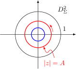
$\overset{\text{mapping}}{\Longrightarrow}$       

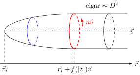
Figure 2: The map from worldsheet disk to the one in space-time.

One should remember that the instanton calculus in the GLSM setup is performed in the limit $g\to 0$ [10]. This limit implies that the cigar defined on the single-centered Taub-NUT space is closed at infinity. Therefore the cigar in this limit becomes topologically $S^{2}$. Schematically we have the following relation:

$$[\text{Disk instanton}]\quad\xrightarrow[g\to 0]{}\quad[\text{Worldsheet instanton}].$$ (4.11)

4.2 Worldsheet instanton corrections to the $5^{2}_{2}$-brane geometry

Following the discussion in the previous subsection, we proceed to the $5^{2}_{2}$-brane geometry [4]:

$$ds^{2}=dx^{2}_{012345}+Hdx^{2}_{67}+HK^{-1}((dx^{8})^{2}+(dx^{9})^{2}),$$

$$H=h_{0}+\sigma\log\frac{\mu}{\rho},\quad\rho^{2}=(x^{6})^{2}+(x^{7})^{2},$$

$$B_{89}=K^{-1}A_{8},\quad K=H^{2}+A_{8}^{2},\quad e^{2\phi}=HK^{-1},$$

$$A_{8}=c\ \text{arctan}\left(\frac{x^{7}}{x^{6}}\right)+\text{const.},$$ (4.12)

where $h_{0},\sigma,\mu,c$ are constants. Now there are two isometries defined in the $x^{8,9}$-directions. The situation is similar to the one in the Taub-NUT space, i.e. the two-torus $T^{2}=S^{1}\times S^{1}$ is fibered over the two-dimensional space $\mathbb{R}^{2}$. The physical radius of each $S^{1}$ is given by $HK^{-1}$. At the origin $\rho\to 0$ in the $x^{6,7}$-plane, we have $HK^{-1}\to 0$, while at the cutoff scale $\rho=\mu$, $HK^{-1}=\frac{h_{0}}{h_{0}^{2}+A_{8}^{2}}<\infty$ is finite provided the constant $h_{0}$ is finite. Therefore, the volume of the fibered torus vanishes at the origin. We find that the two circles $S_{i}^{1}\ (i=1,2)$ are separately fibered over a segment defined between $\rho=\rho_{0}=0$ and the cutoff surface $\rho=\mu$ in the $x^{6,7}$-plane. Here $i=1,2$ labels the two circle directions $x^{8},x^{9}$.

Since the one-dimensional homology group of the two torus is $H_{1}(T^{2})=\mathbb{Z}\oplus\mathbb{Z}$, a general one-cycle in $T^{2}$ is generated by two integers. There are two independent one-cycles in each $S^{1}$ in $T^{2}=S^{1}\times S^{1}$. One can then define a one-cycle by a formal linear combination of these two one-cycles. For example, a one-dimensional string that wraps on the first $S^{1}$ $n_{1}$-times and the second $S^{1}$ $n_{2}$-times defines a one-cycle in $T^{2}$. We call this the $(n_{1},n_{2})$-cycle which is completely classified by two integers. Analogous to the Taub-NUT case, this $(n_{1},n_{2})$-cycle is fibered over the segment $\rho\in[0,\mu]$ and defines an open cigar. This naturally induces a map from the worldsheet disk $D^{2}_{\Sigma}$ to the disk $D^{2}$ defined over the $(n_{1},n_{2})$-cycle fibration:

$$D^{2}_{\Sigma}=\left\{z\in\mathbb{C}:|z|<1\right\}$$

$$\longrightarrow(n_{1},n_{2})C=\left\{\vec{\rho}(z)=\vec{\rho}_{0}+f(|z|)\vec{v},\ x^{8}(z)=n_{1}\text{arg}(z),x^{9}(z)=n_{2}\text{arg}(z)\right\},$$

$$f(0)=0,\quad f(1)=\mu.$$ (4.13)

Namely, when one goes around the origin inside the worldsheet disk, the map winds the first $S^{1}$ $n_{1}$-times and the second $S^{1}$ $n_{2}$-times. This fact substantially leads to a generalization of the disk instantons. See Figure 3.

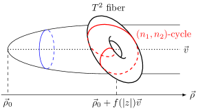
Figure 3: Open cigar in the $5^{2}_{2}$-brane geometry whose boundary is given by the $(n_{1},n_{2})$-cycle.

If we consider the limit $h_{0}\to\infty$, then the two open cigars $D^{2}_{i}$ are closed at $\rho\sim\mu$ forming $S^{2}_{i}$. It is therefore obvious that the map is classified by the homotopy group $\pi_{2}(S^{2}_{1})\oplus\pi_{2}(S^{2}_{2})=\mathbb{Z}\oplus\mathbb{Z}$.

In order to justify the above homotopy assignment and define the topological charges, we examine the homology structure of the two-cycles. Since we have the Betti number $b_{2}(S^{2})=1$, we can define a harmonic $(1,1)$-form $b^{i}(i=1,2)$ in each $S^{2}_{i}$ for which we have the period matrix:

$$\int_{S^{2}_{i}}b^{j}=\tilde{R}_{i}^{-1}\delta_{i}{}^{j},\quad(\text{$i$: no sum}).$$ (4.14)

Here $\tilde{R}_{i}$ are constants. Then the Kähler form $\Omega$ is expanded by

$$\Omega=\sum_{i=1,2}c_{i}b^{i},$$ (4.15)

where $c_{i}$ are real constants. On the other hand, corresponding to the $(n_{1},n_{2})$-cycle, we can associate a linear combination of closed cigar $S^{2}=n_{1}S^{2}_{1}+n_{2}S^{2}_{2}$. Utilizing these facts, the BPS bound of the worldsheet Polyakov action is given by

$$S\geq\frac{1}{4\pi\alpha^{\prime}}\vec{c}\cdot\vec{Q},$$ (4.16)

where $\vec{c}=(c_{1},c_{2})$, $\vec{Q}=(Q^{1},Q^{2})$ and

$$Q^{i}=\int_{\Sigma}\phi^{*}(b^{i})=\int_{\phi(\Sigma)}b^{i}=\frac{n_{i}}{\tilde{R}_{i}},$$ (4.17)

where we have used $\phi(\Sigma)=n_{1}S^{2}_{1}+n_{2}S^{2}_{2}$ and the relation (4.14). This is the topological charge [38, 39] associated with the map defined above. The most stringent bound of the action is found to be

$$S\geq\frac{1}{4\pi\alpha^{\prime}}|\vec{c}|\sqrt{\left(\frac{n_{1}}{\tilde{R}_{1}}\right)^{2}+\left(\frac{n_{2}}{\tilde{R}_{2}}\right)^{2}}.$$ (4.18)

This bound is saturated when the condition (4.3) is satisfied and the vector $\vec{c}$ is parallel to $\vec{Q}$. Introducing the contribution of the Kalb-Ramond field, we have the instanton action (where we have chosen the plus sign in (4.4)):

$$S_{\text{inst.}}=\frac{1}{4\pi\alpha^{\prime}}\left[|\vec{c}|\sqrt{\left(\frac{n_{1}}{\tilde{R}_{1}}\right)^{2}+\left(\frac{n_{2}}{\tilde{R}_{2}}\right)^{2}}-i\vec{n}\cdot\vec{\mathcal{B}}\right].$$ (4.19)

Here

$$\mathcal{B}^{i}=-\int_{\phi^{*}(S^{2}_{i})}\!d^{2}\sigma\,B_{\mu}{}^{\rho}\,\Omega_{\rho\nu}\,\partial^{a}X^{\mu}\partial_{a}X^{\nu}.$$ (4.20)

Assigning $|\vec{c}|$ the distance scale $\rho$, we find the precise agreement between $e^{-S_{\text{inst.}}}$ and the exponential factor appeared in (3.15). This is a conceivable result.

One then proceeds the cases with more isometries, for example, the $5^{3}_{2}$-branes ($R$-brane). The discussion is completely parallel. For example, the geometry of the $5^{3}_{2}$-branes includes $T^{3}$-fibration over $\mathbb{R}$. The homology $H_{1}(T^{3})=\mathbb{Z}\oplus\mathbb{Z}\oplus\mathbb{Z}$ indicates that disk instantons are labelled by three integers $(n_{1},n_{2},n_{3})$. Indeed, we can define a generalization of the map (4.9) and we deduce that instanton action agrees with the exponential factor appeared in (3.19). The same is true for the DFT wave solutions. However, this picture fails when we move to space-filling branes. There are no non-trivial base space in this case. Therefore, there is no straightforward way to generalize the discussion to space-filling branes.

5 Instantons in GLSM

In this section, we consider the worldsheet instantons in the GLSM language. The explicit instanton calculus was first performed in [9] in which, in order to realize the H-monopole geometry, the two-dimensional $\mathcal{N}=(4,4)$ vector, hyper and twisted hypermultiplets are prepared. The gauge group is $U(1)$ which has a direct connection to the isometry of the H-monopole. As we have mentioned before, the instanton calculus is justified only when the sigma model coupling is small $g\to 0$. In this limit, the GLSM is reduced to a truncated model. For the GLSMs describing the H-monopole and KK-monopole, the truncated model is given by the Abelian-Higgs model. Instantons in the GLSM is the BPS vortices associated with the $U(1)$ gauge field [9]. This is indeed the case for the $5^{2}_{2}$-brane geometry [13, 14].

Now we consider GLSM describing geometries with $T^{N}$-fibration. Since the isometry of the background geometry is encoded into the gauge symmetry in the GLSM, we assume that a conceivable gauge group is $G=U(1)\times U(1)\times\cdots=U(1)^{N}$ which is associated with the isometry in $T^{N}$. Following the previous works for the H-, KK-monopoles and $5^{2}_{2}$-brane, we also assume that the truncated model in an appropriate limit of parameters is given by the $(2+0)$-dimensional Abelian-Higgs model,

$$\mathcal{L}_{\text{E}}=\sum_{a=1}^{N}\left[\frac{1}{2e_{a}^{2}}(F_{12,a})^{2}+|D_{m}q_{a}|^{2}+\frac{e_{a}^{2}}{2}\left(|q_{a}|^{2}-\sqrt{2}\,\zeta_{a}\right)^{2}+i\sqrt{2}\,\vartheta_{a}F_{12,a}\right].$$ (5.1)

Here $A_{m,a}\ (m=1,2;a=1,\ldots,N)$ are the $U(1)$ gauge fields, $q_{a}$ are charged scalar fields, $\zeta_{a}$ are the Fayet-Iliopoulos (FI) parameters associated with each $U(1)$ sector. The covariant derivatives and the gauge field strength are given as $D_{m}q_{a}=\partial_{m}q_{a}+iA_{m,a}q_{a}\ (m=1,2;a:\text{no sum})$ and $F_{12,a}=\partial_{1}A_{2,a}-\partial_{2}A_{1,a}$, respectively. The last term is a topological term for which $\vartheta_{a}\ (a=1,2,\ldots,N)$ is scalar fields corresponding to the winding coordinates. For the KK-monopole and $5^{2}_{2}$-brane cases, the charged scalar field comes from the hypermultiplet while the scalar field $\vartheta$ is a “remnant” of the twisted hypermultiplet presented in the GLSM for the H-monopole. It has been shown that the topological term including $\vartheta$ is left behind in the process of the T-duality transformation [40]. In the T-dualized frame, this $\vartheta$ can be interpreted as the dual coordinate. In other words, this is the GLSM origin of the winding coordinate dependence of geometries.

It is easy to find the Bogomol’nyi bound of the Euclidean Lagrangian (5.1). We find

$$\mathcal{L}_{\text{E}}\geq \ \mp\sqrt{2}\sum_{a}\zeta_{a}F_{12,a}+i\sqrt{2}\sum_{a}\vartheta_{a}F_{12,a}+\text{(total derivative)}.$$ (5.2)

If we define $\vec{\zeta}=(\zeta_{a=1},\zeta_{a=2},\ldots)$, $\vec{\vartheta}=(\vartheta_{a=1},\vartheta_{a=2},\ldots)$, $\vec{F}_{12}=(F_{12,a=1},F_{12,a=2},\ldots)$, and $\vec{Q}\equiv-\frac{1}{2\pi}\int\!d^{2}x\ \vec{F}_{12}$, the most stringent bound of the Euclidean action $S_{\text{E}}=\frac{1}{2\pi}\int\!d^{2}x\ \mathcal{L}_{\text{E}}$ is

$$S_{\text{E}}\geq \ \sqrt{2}|\vec{\zeta}|\sqrt{\sum_{a}Q_{a}^{2}}-i\sqrt{2}\,\vec{\vartheta}\cdot\vec{Q}.$$ (5.3)

Here the equality is saturated when the FI parameter $\vec{\zeta}$ and $\vec{Q}$ becomes parallel $\vec{\zeta}\parallel\vec{Q}$ and the following BPS equations hold:

$$F_{12,a}\mp e_{a}^{2}(|q_{a}|^{2}-\sqrt{2}\,\zeta_{a})=0,\quad D_{1}q_{a}\pm iD_{2}q_{a}=0,\qquad a=1,2,\ldots,N.$$ (5.4)

The equations (5.4) are nothing but the Abrikosov-Nielsen-Olesen (ANO) vortex equations in each $U(1)$ sector ($a=1,2,\ldots,N$). They are independent equations and give the non-trivial first Chern numbers specified by the homotopy group $\pi_{1}(G)=\pi_{1}(S^{1})\oplus\pi_{1}(S^{1})\oplus\cdots\simeq\mathbb{Z}^{N}$. The topological charges are given by

$$\vec{Q}=(n_{1},n_{2},\ldots,n_{N}),\quad n_{a}\in\mathbb{Z},\qquad a=1,\ldots,N.$$ (5.5)

The path integral on the solution to (5.4) is calculated by the integral over the moduli space $\mathcal{M}_{n_{1},n_{2},\ldots,n_{N}}$ of each ANO vortex. Rescaling the gauge field $A_{m,a}\to\frac{1}{\tilde{R}_{a}}A_{m,a}$ and taking into account the overall factor and rewrite $\vartheta_{a}\equiv\tilde{x}_{a}$, $|\vec{\zeta}|\equiv\rho$ [9], we obtain (we have chosen the plus sign in (5.4))

$$Z=\sum_{n_{1},n_{2},\ldots,n_{N}}\int\!d\mathcal{M}_{n_{1},\ldots,n_{N}}\exp\left[-\rho\sqrt{\left(\frac{n_{1}}{\tilde{R}_{1}}\right)^{2}+\left(\frac{n_{2}}{\tilde{R}_{2}}\right)^{2}+\cdots}+i\left(n_{1}\frac{\tilde{x}_{1}}{\tilde{R}_{1}}+n_{2}\frac{\tilde{x}_{2}}{\tilde{R}_{2}}+\cdots\right)+\cdots\right],$$ (5.6)

where the last $\cdots$ in the exponential factor stands for the moduli of the vortices. This again produces the characteristic structure appeared in (3.15). Therefore the winding corrections found in the DFT solutions are expected to be realized as vortex corrections in GLSM. The related group structures of the instantons are found in Table 2.

	KK-monopole	$5^{2}_{2}$-brane
Fibration	$S^{1}$ over $\mathbb{R}^{3}$	$T^{2}=S^{1}\times S^{1}$ over $\mathbb{R}^{2}$
Homology	$H_{1}(S^{1})=\mathbb{Z}$	$H_{1}(T^{2})=\mathbb{Z}\oplus\mathbb{Z}$
NLSM homotopy	$\pi_{2}(S^{2})=\mathbb{Z}$	$\pi_{2}(S^{2})\oplus\pi_{2}(S^{2})=\mathbb{Z}\oplus\mathbb{Z}$
GLSM homotopy	$\pi_{1}(U(1))=\mathbb{Z}$	$\pi_{1}(U(1)^{2})=\mathbb{Z}\oplus\mathbb{Z}$

Table 2: Related group structures of the instantons in NLSM and GLSM.

Finally, we comment on the complete description of the Lagrangian. In this paper we focused only on the topological structure of the target space, i.e., we neglected any contributions from F-terms which play a significant role in constructing supersymmetric theory and describing the target space geometry. Since the target space is a T-dualized version of the Taub-NUT space, the gauge theory must have ${\cal N}=(4,4)$ supersymmetry which requires $SU(2)$ R-symmetry. However, more than one topological terms such as $\sum_{a}\vartheta_{a}F_{12,a}$ would break the $SU(2)$ R-symmetry to $U(1)$, hence the ${\cal N}=(4,4)$ supersymmetry is broken to ${\cal N}=(2,2)$ at least in the classical level. The reason is as follows. We begin with the GLSM for five-branes [9] (and series of works [13, 14, 41, 42, 43, 44, 45]). Four transverse directions of the five-branes are represented by four scalars belonging to the twisted hypermultiplet. $\vartheta_{a}$ is chosen as one component of this multiplet. The remaining three scalars belong to a triplet of the $SU(2)$ R-symmetry. If one introduces another topological term associated with another $\vartheta_{b}$, this requires a different $SU(2)$ triplet which conflicts with the original one. However, since we regard the GLSM as string worldsheet theory and its UV completion, we believe that the broken supersymmetry must be restored in the IR limit.

6 Conclusion and discussions

In this paper we have studied string winding corrections to the five-brane, F-string and wave geometries. We have explored classical DFT solutions of five-branes. The solutions are classified according to the codimensions of the branes in supergravity. For example, applying the formal $O(d,d)$ transformations to the NS5-brane of codimension four, we have found new solutions that depend on multiple winding coordinates. These include the KK-monopole with one winding, the $5^{2}_{2}$-brane with two windings and the $R$-brane with three winding coordinates dependence. The solution generating technique is also available even for lower codimensional cases. Starting from the H-monopole (codimension three) and smeared H-monopoles (codimension two and one), we have shown various five-brane solutions that involve winding coordinate dependency. We have also written down codimension zero, space-filling five-branes that are fully localized in the winding space. Although they inevitably have trivial geometry (flat space-time) in the supergravity language, they inherit non-trivial structures in the winding space.

We have also worked out the winding solutions based on the DFT wave solution. The analysis presented in this paper reveals that there are winding corrections even for the F-string and wave solutions. Although some of the solutions have been mentioned and found in the literature [17, 18, 19, 29, 32], our systematic analysis makes it clear that for a given supergravity solution in the NSNS sector, we can explicitly written down all the T-dualized solutions that depend on the winding coordinates.

In the latter half of this paper, we have discussed a physical interpretation of the winding solutions. We have separated out the winding sector from the ordinary supergravity solutions. For solutions of less than two codimensions, the zero-winding sectors diverge but they can be subtracted. Except for the space-filling branes, we have elucidated the exponential behaviors of the winding coordinate dependence of the solutions. These characteristic structures suggest that they originate from instanton effects.

We have then discussed an interpretation of the winding corrections as string worldsheet instanton effects. Based on the notion of the disk instantons in the single-centered Taub-NUT space [37], we have generalized it to the $5^{2}_{2}$-brane geometry. In an appropriate limit of parameters, a disk in the target space is closed and the disk instantons are promoted to the well-defined worldsheet instantons. The map from the worldsheet to the target geometry is classified according to the set of homotopy groups and the map is labeled by integers associated with winding numbers. Assuming that the Euclidean worldsheet action is minimized, we have reproduced the correct exponential behavior that appeared in the DFT winding solutions. We have also given a discussion on the instanton effects based on the GLSM language. It is known that the worldsheet instantons are well described by the GLSM formalism [9]. The worldsheet instantons are represented by the ANO vortices in the GLSM. Indeed, the winding corrections to the KK-monopole geometry (3.8) is precisely reproduced by the path integral over the vortex moduli space [10]. Related to this issue, two of the authors studied the instanton corrections to the geometry of the exotic $5^{2}_{2}$-brane [13, 14]. Again it has been discussed that the ANO vortices induces instanton corrections whose effect sums up to the one given in (3.14). With these observations, it is plausible that the multiple winding dependence of the geometries is captured by the ANO vortices associated with the $U(1)^{N}$ gauge symmetry in the GLSM. We have a qualitative discussion on this issue. Assuming the copies of the Abelian-Higgs model as a truncated model in a limit of geometric parameters (this guarantees the instanton interpretation), we have again reproduced the characteristic exponential structure appearing in the harmonic function.

DFT is a framework where the $O(d,d)$ T-duality symmetry is manifest. It is naturally generalized to the exceptional field theory (EFT) [46], the U-duality covariant formulation, for which not only the NSNS sector but also the RR sector of superstring theory are included. Several classical solutions for branes including D-branes in EFT are studied [47]. Analogous to the DFT solutions presented here, it is discussed that there are also EFT solutions that include “dual coordinate dependence” [48]. Related works on the winding corrections in the semi-flat elliptic metric is analyzed in [32, 49]. Since the type II supergravity is manifestly included in EFT, our analysis leads to the following conjecture:

If there is a classical solution to conventional type II supergravity theories, one obtains associated DFT (EFT) solutions that depend on the dual coordinates by formally applying T(U)-duality transformations to the solution. Namely, there are always string winding corrections to every known supergravity solution.

The appearance of the dual coordinates in EFT solutions is a consequence of windings of various branes. It is therefore natural to interpret it as instanton effects originating from wrapped branes on some cycles.

Since it is necessary to use the GLSM technique for the quantitative analysis of the instanton effects, it is interesting to construct the complete GLSM action that have $U(1)^{N}$ gauge symmetry. It is also interesting to study the winding corrections to geometries from the viewpoint of the worldvolume theories of exotic branes [50, 51, 52, 53]. It is interesting to study the winding corrections to the five-branes in heterotic theories [54, 55]. We will come back to these issues in future works.

Acknowledgments

The work of T. K. is supported by the Iwanami-Fujukai Foundation. The work of S. S. is supported by the Japan Society for the Promotion of Science (JSPS) KAKENHI Grant Number JP17K14294 and Kitasato University Research Grant for Young Researchers.

References

- [1] N. A. Obers and B. Pioline, “U-duality and M-theory,” Phys. Rept. 318 (1999) 113 [hep-th/9809039].
- [2] S. Hellerman, J. McGreevy and B. Williams, “Geometric constructions of nongeometric string theories,” JHEP 0401 (2004) 024 [hep-th/0208174].
- [3] J. Shelton, W. Taylor and B. Wecht, “Nongeometric flux compactifications,” JHEP 0510 (2005) 085 [hep-th/0508133].
- [4] J. de Boer and M. Shigemori, “Exotic branes and non-geometric backgrounds,” Phys. Rev. Lett. 104 (2010) 251603 [arXiv:1004.2521 [hep-th]], “Exotic branes in string theory,” Phys. Rept. 532 (2013) 65 [arXiv:1209.6056 [hep-th]].
- [5] C. M. Hull, “Doubled geometry and T-folds,” JHEP 0707 (2007) 080 [hep-th/0605149].
- [6] F. Haßler and D. Lüst, “Non-commutative/non-associative IIA (IIB) - and -branes and their intersections,” JHEP 1307 (2013) 048 [arXiv:1303.1413 [hep-th]].
- [7] Y. Sakatani, “Exotic branes and non-geometric fluxes,” JHEP 1503 (2015) 135 [arXiv:1412.8769 [hep-th]].
- [8] D. Andriot and A. Betz, “NS-branes, source corrected Bianchi identities, and more on backgrounds with non-geometric fluxes,” JHEP 1407 (2014) 059 [arXiv:1402.5972 [hep-th]].
- [9] D. Tong, “NS5-branes, T-duality and worldsheet instantons,” JHEP 0207 (2002) 013 [hep-th/0204186].
- [10] J. A. Harvey and S. Jensen, “Worldsheet instanton corrections to the Kaluza-Klein monopole,” JHEP 0510 (2005) 028 [hep-th/0507204].
- [11] S. Jensen, “The KK-monopole/NS5-brane in doubled geometry,” JHEP 1107 (2011) 088 [arXiv:1106.1174 [hep-th]].
- [12] R. Gregory, J. A. Harvey and G. W. Moore, “Unwinding strings and T-duality of Kaluza-Klein and H-monopoles,” Adv. Theor. Math. Phys. 1 (1997) 283 [hep-th/9708086].
- [13] T. Kimura and S. Sasaki, “Gauged linear sigma model for exotic five-brane,” Nucl. Phys. B 876 (2013) 493 [arXiv:1304.4061 [hep-th]].
- [14] T. Kimura and S. Sasaki, “Worldsheet instanton corrections to -brane geometry,” JHEP 1308 (2013) 126 [arXiv:1305.4439 [hep-th]].
- [15] C. Hull and B. Zwiebach, “Double field theory,” JHEP 0909 (2009) 099 [arXiv:0904.4664 [hep-th]].
- [16] W. Siegel, “Two vierbein formalism for string inspired axionic gravity,” Phys. Rev. D 47 (1993) 5453 [hep-th/9302036], “Superspace duality in low-energy superstrings,” Phys. Rev. D 48 (1993) 2826 [hep-th/9305073], “Manifest duality in low-energy superstrings,” hep-th/9308133.
- [17] J. Berkeley, D. S. Berman and F. J. Rudolph, “Strings and branes are waves,” JHEP 1406 (2014) 006 [arXiv:1403.7198 [hep-th]].
- [18] D. S. Berman and F. J. Rudolph, “Branes are waves and monopoles,” JHEP 1505 (2015) 015 [arXiv:1409.6314 [hep-th]].
- [19] I. Bakhmatov, A. Kleinschmidt and E. T. Musaev, “Non-geometric branes are DFT monopoles,” JHEP 1610 (2016) 076 [arXiv:1607.05450 [hep-th]].
- [20] A. Dabholkar and C. Hull, “Generalised T-duality and non-geometric backgrounds,” JHEP 0605 (2006) 009 [hep-th/0512005].
- [21] V. Vall Camell, “NS5 duals in supergravity and double field theory,” PoS CORFU 2016 (2017) 114.
- [22] O. Hohm, C. Hull and B. Zwiebach, “Generalized metric formulation of double field theory,” JHEP 1008 (2010) 008 [arXiv:1006.4823 [hep-th]].
- [23] C. G. Callan, Jr., J. A. Harvey and A. Strominger, “Worldsheet approach to heterotic instantons and solitons,” Nucl. Phys. B 359 (1991) 611.
- [24] T. H. Buscher, “A symmetry of the string background field equations,” Phys. Lett. B 194 (1987) 59, “Path integral derivation of quantum duality in nonlinear sigma models,” Phys. Lett. B 201 (1988) 466.
- [25] X. C. de la Ossa and F. Quevedo, “Duality symmetries from non-Abelian isometries in string theory,” Nucl. Phys. B 403 (1993) 377 [hep-th/9210021].
- [26] T. Kugo and B. Zwiebach, “Target space duality as a symmetry of string field theory,” Prog. Theor. Phys. 87 (1992) 801 [hep-th/9201040].
- [27] E. A. Bergshoeff, T. Ortín and F. Riccioni, “Defect branes,” Nucl. Phys. B 856 (2012) 210 [arXiv:1109.4484 [hep-th]].
- [28] V. K. Onemli and B. Tekin, “Kaluza-Klein vortices,” JHEP 0101 (2001) 034 [hep-th/0011287].
- [29] C. D. A. Blair, “Doubled strings, negative strings and null waves,” JHEP 1611 (2016) 042 [arXiv:1608.06818 [hep-th]].
- [30] A. Sen, “Kaluza-Klein dyons in string theory,” Phys. Rev. Lett. 79 (1997) 1619 [hep-th/9705212].
- [31] T. Kikuchi, T. Okada and Y. Sakatani, “Rotating string in doubled geometry with generalized isometries,” Phys. Rev. D 86 (2012) 046001 [arXiv:1205.5549 [hep-th]].
- [32] D. Lüst, E. Plauschinn and V. Vall Camell, “Unwinding strings in semi-flatland,” JHEP 1707 (2017) 027 [arXiv:1706.00835 [hep-th]].
- [33] E. A. Bergshoeff, O. Hohm, V. A. Penas and F. Riccioni, “Dual double field theory,” JHEP 1606 (2016) 026 [arXiv:1603.07380 [hep-th]].
- [34] X. G. Wen and E. Witten, “World-sheet instantons and the Peccei-Quinn symmetry,” Phys. Lett. 166B (1986) 397.
- [35] E. Witten, “Phases of theories in two-dimensions,” Nucl. Phys. B 403 (1993) 159 [AMS/IP Stud. Adv. Math. 1 (1996) 143] [hep-th/9301042].
- [36] E. Witten, “Small instantons in string theory,” Nucl. Phys. B 460 (1996) 541 [hep-th/9511030].
- [37] K. Okuyama, “Linear sigma models of H and KK monopoles,” JHEP 0508 (2005) 089 [hep-th/0508097].
- [38] P. J. Ruback, “ model solitons and their moduli space metrics,” Commun. Math. Phys. 116 (1988) 645.
- [39] M. Dine, N. Seiberg, X. G. Wen and E. Witten, “Nonperturbative effects on the string world sheet. 2,” Nucl. Phys. B 289 (1987) 319.
- [40] M. Roček and E. P. Verlinde, “Duality, quotients, and currents,” Nucl. Phys. B 373 (1992) 630 [hep-th/9110053].
- [41] T. Kimura and S. Sasaki, “Worldsheet description of exotic five-brane with two gauged isometries,” JHEP 1403 (2014) 128 [arXiv:1310.6163 [hep-th]].
- [42] T. Kimura and M. Yata, “T-duality transformation of gauged linear sigma model with F-term,” Nucl. Phys. B 887 (2014) 136 [arXiv:1406.0087 [hep-th]].
- [43] T. Kimura, “ gauged linear sigma models for defect five-branes,” arXiv:1503.08635 [hep-th].
- [44] T. Kimura, “Gauge-fixing condition on prepotential of chiral multiplet for nongeometric backgrounds,” PTEP 2016 (2016) no.2, 023B04 [arXiv:1506.05005 [hep-th]].
- [45] T. Kimura, “Semi-doubled sigma models for five-branes,” JHEP 1602 (2016) 013 [arXiv:1512.05548 [hep-th]].
- [46] O. Hohm and H. Samtleben, “Exceptional form of supergravity,” Phys. Rev. Lett. 111 (2013) 231601 [arXiv:1308.1673 [hep-th]].
- [47] D. S. Berman and F. J. Rudolph, “Strings, branes and the self-dual solutions of exceptional field theory,” JHEP 1505 (2015) 130 [arXiv:1412.2768 [hep-th]].
- [48] I. Bakhmatov, D. Berman, A. Kleinschmidt, E. Musaev and R. Otsuki, “Exotic branes in exceptional field theory: the duality group,” JHEP 1808 (2018) 021 [arXiv:1710.09740 [hep-th]].
- [49] I. Achmed-Zade, M. J. D. Hamilton, D. Lüst and S. Massai, “A note on T-folds and fibrations,” JHEP 1812 (2018) 020 [arXiv:1803.00550 [hep-th]].
- [50] A. Chatzistavrakidis, F. F. Gautason, G. Moutsopoulos and M. Zagermann, “Effective actions of nongeometric five-branes,” Phys. Rev. D 89 (2014) no.6, 066004 [arXiv:1309.2653 [hep-th]].
- [51] T. Kimura, S. Sasaki and M. Yata, “World-volume effective actions of exotic five-branes,” JHEP 1407 (2014) 127 [arXiv:1404.5442 [hep-th]].
- [52] T. Kimura, S. Sasaki and M. Yata, “World-volume effective action of exotic five-brane in M-theory,” JHEP 1602 (2016) 168 [arXiv:1601.05589 [hep-th]].
- [53] C. D. A. Blair and E. T. Musaev, “Five-brane actions in double field theory,” JHEP 1803 (2018) 111 [arXiv:1712.01739 [hep-th]].
- [54] S. Sasaki and M. Yata, “Non-geometric five-branes in heterotic supergravity,” JHEP 1611 (2016) 064 [arXiv:1608.01436 [hep-th]].
- [55] S. Sasaki and M. Yata, “Gauge five-brane solutions of co-dimension two in heterotic supergravity,” JHEP 1710 (2017) 214 [arXiv:1708.08066 [hep-th]].