No-Go theorems for ekpyrosis from ten-dimensional supergravity

Abstract:

In this note we investigate whether the new ekpyrotic scenario can be embedded into ten-dimensional supergravity. We use that the scalar potential obtained from flux compactifications of type II supergravity with sources has a universal scaling with respect to the dilaton and the volume mode. Similar to the investigation of inflationary models, we find very strong constraints ruling out ekpyrosis from analysing the fast-roll conditions. We conclude that flux compactifications tend to provide potentials that are neither too flat and positive (inflation) nor too steep and negative (ekpyrosis).

1 Introduction

The strong no-go theorems which exclude tree-level de Sitter compactifications under a few simple assumptions with or without negative tension objects such as orientifold planes have been much explored because of the possible cosmological and phenomenological interests. However, the no-go theorems for ekpyrotic scenario which is alternative to inflation model in string theory is much less extensive. One motivation for the present work is to improve this situation. Since orientifold planes are a common ingredient in phenomenologically interesting type II string theory, it seems natural to explore the possibility of treelevel de Sitter vacua or inflation models in type II string theory with orientifolds. On the other hand, there is no constraint for ekpyrotic scenario in type II string theory at present.

The ekpyrosis inspired by string theory and brane world model suggests alternative solutions to the early universe puzzles such as inflation and dark energy, and assumes that two four-dimensional boundary branes which are located at the endpoints of orbifold in the higher-dimensional bulk spacetime [1, 2, 3, 4, 5, 6]. For brane world picture, all forces except for gravity are localized on the branes while gravity can propagate freely in the bulk. When we assume that there is an attractive force between two branes, these branes approach to each other, which gives big bang. Since the big bang is described as a collision of branes there is not the beginning of time in the ekpyrotic scenario. Although two branes move through each other at once after collision, we can get a model so that the branes become closer again.

The motion of branes is described by the potential of scalar field in a four-dimensional effective theory. Non-perturbative effects result in a potential which attracts one brane towards the other brane [1]. In order to resolve a horizon and flatness problem, the potential during a period of slow contraction before the big bang is negative and steeply falling. There was plenty of time before the big bang for the universe to be in causal contact over large regions, and in this way the horizon and flatness problem is automatically solved [4]. Then, the usual statement of the ekpyrosis is that the universe slowly contracts before the big bang with the equation of state $w=p/\rho\gg 1$ . The scalar potential is expected to turn up towards zero at large negative value of scalar field in the ekpyrotic or cyclic models.

As two branes approach each other, the branes are rippled because of generating quantum fluctuations. Since the collision of branes cannot be happened at exactly the same time, the branes collide slightly earlier or later in some places. Our universe thus has a little bit more time to cool or hot. When we consider the curvature perturbation in the ekpyrotic scenario, it occurs a strong blueshift, which is in sharp contradiction with the small redshift of the scalar fluctuation in the CMB [7, 8, 9, 10, 11, 12, 13, 14, 15]. The occurrence of blueshift scalar perturbation is nonetheless a minor flaw of ekpyrotic theory which can be easily corrected. Hence, new ekpyrotic theory considers multiple scalar field and successfully generated a scalar spectrum which is scale invariant and slightly redshifted [16, 17, 18, 19, 20, 21, 22, 23, 24, 25, 26, 27, 28, 29, 30]. Producing primordial gravitational waves sourced by the gauge field in the ekpyrotic scenario was also studied in [31].

It is the purpose of this note to give a No-Go theorem of the ekpyrotic scenario in a ten-dimensional supergravity model which is low energy limit of a string theory. We study the dynamics of two scalar fields in the four-dimensional effective theory after a compactification in string theory. There are a dilaton and the volume modulus of the internal manifold in the effective theory, which is a four-dimensional theory of gravity minimally coupled to two-scalar fields. We will derive the two moduli fields with negative exponential potentials. Since this potential is steep, the scalar field should be satisfied by “fast-roll” condition instead of slow-roll parameter in inflation model [32, 33]. Although the terms coupling the scalar fields to the scalar curvature of the internal space and orientifold plane contribute the negative value to the potential in the string theory, we find that the potential does not satisfy the fast-roll condition in general. Therefore, it is not possible for us to realize the ekpyrotic phase in a string theory.

Section 2 describes the potential of scalar field for ekpyrotic scenario and the way it derives the four-dimensional effective theory. We discuss the approach to the effective action in more detail. The No-Go theorem of the ekpyrosis thus given by the string theory is discussed. We also investigate the detailed properties of these models, their embedding in a string theory and their viability. For simplicity, we do not consider D-branes and the associated moduli except for the volume modulus (breathing mode) of internal space although the analysis would not be different.

Finally, section 3 provides a brief summary and an outlook to future developments. We have tried to make the context of this note relatively self-contained, but some details for the derivation of four-dimensional effective action is contained in appendix A.

2 No-Go theorem of the ekpyrotic scenario in the type II theory

In this section, we consider compactifications of the type II theory to four-dimensional spacetime on compact manifold Y. The ten-dimensional low-energy effective action for the type II theory takes the form [34, 35]

$$S = \frac{1}{2\bar{\kappa}^{2}}\int d^{10}x\sqrt{-g}\left[{\rm e}^{-2\phi}\left(R+4g^{MN}\partial_{M}\phi\partial_{N}\phi-\frac{1}{2}\left|H\right|^{2}\right)-\frac{1}{2}\sum_{p}\left|F_{p}\right|^{2}\right]$$ (1)

$$-\sum_{p}\left(T_{{\rm D}p}+T_{{\rm O}p}\right)\int d^{p+1}x\sqrt{-g_{p+1}}\,{\rm e}^{-\phi}\,,$$

where $\bar{\kappa}^{2}$ is the ten-dimensional gravitational constant, $R$ denotes the ten-dimensional Ricci scalar, $\phi$ is the scalar field, $H$ is the NS-NS 3-form field strength, $F_{p}$ are the R-R $p$-form field strengths ($p=0,2,4,6,8$ for type IIA, and $p=1,3,5,7,9$ for type IIB) that are sourced by D-branes, and $T_{{\rm D}p}$ $(T_{{\rm O}p})$ is the D$p$-brane (O$p$-plane) charge and tension. Although there are Chern-Simons terms in the ten-dimensional action, these are essentially independent of the dilaton and the scale of the background metric. Hence, we will not consider them.

To compactify the theory to four dimensions, we consider the a metric ansatz of the form [34, 35]

$$ds^{2} = g_{MN}dx^{M}dx^{N}=q_{\mu\nu}dx^{\mu}dx^{\nu}+g_{ij}dy^{i}dy^{j}$$ (2)

$$= q_{\mu\nu}dx^{\mu}dx^{\nu}+\rho\,u_{ij}({\rm Y})dy^{i}dy^{j}\,,$$

where $\rho$ is breathing mode (volume modulus of the compact space), $x^{\mu}$ denote the coordinates of four-dimensional spacetime, $y^{i}$ are local coordinates on the internal space Y, and $g_{MN}$ , $q_{\mu\nu}$ , $u_{ij}({\rm Y})$ are the metric of ten-dimensional spacetime, four-dimensional spacetime, six-dimensional internal space, respectively. We assume that $q_{\mu\nu}$ , $u_{ij}$ depend only on the coordinates $x^{\mu}$, $y^{i}$ , respectively. Since we factored out the overall volume modulus (breathing mode) $\rho$ of the internal space in the ten-dimensional metric (2), the modulus $\rho$ is related to the total physical volume of the internal space $v_{6}$ and the volume of Y space $v({\rm Y})$ as

$$\rho=\left[\frac{v_{6}}{v({\rm Y})}\right]^{1/3}\,,~{}~{}~{}~{}~{}v_{6}=\int d^{6}y\sqrt{g_{6}}\,,~{}~{}~{}~{}~{}v({\rm Y})=\int d^{6}y\sqrt{u}\,.$$ (3)

Here, $g_{6}$ , $u$ denote the determinant of the metric $g_{ij}$ , $u_{ij}({\rm Y})$ , respectively . The volume modulus $\rho$ is chosen such that the metric $u_{ij}({\rm Y})$ of the internal space is normalized $v({\rm Y})=1$ .

After we integrate over the internal space Y, the four-dimensional effective action $S_{\rm E}$ in the Einstein frame is given by

$$S_{\rm E} = \frac{1}{2\kappa^{2}}\int d^{4}x\sqrt{-\bar{q}}\left[\bar{R}-\frac{3}{2}\bar{q}^{\mu\nu}\partial_{\mu}\ln\rho\,\partial_{\nu}\ln\rho-2\bar{q}^{\mu\nu}\partial_{\mu}\ln\tau\,\partial_{\nu}\ln\tau\right.$$ (4)

$$+\left(\frac{\bar{\kappa}}{\tau\kappa}\right)^{2}\rho^{-1}R({\rm Y})-\frac{1}{2}\left(\frac{\bar{\kappa}}{\tau\kappa}\right)^{2}\rho^{-3}\left|H\right|^{2}-\frac{1}{2}\sum_{p}\left(\frac{\bar{\kappa}}{\tau^{2}\kappa}\right)^{2}\rho^{3-p}\left|F_{p}\right|^{2}$$

$$\left.-2\sum_{p}\left(T_{{\rm D}p}+T_{{\rm O}p}\right)\left(\frac{\bar{\kappa}^{2}}{\kappa}\right)^{2}\tau^{-3}\rho^{(p-6)/2}\int d^{p-3}x\sqrt{g_{p-3}}\,\right],$$

where $R({\rm Y})$ denotes the Ricci scalar constructed from the metric $u_{ij}({\rm Y})$  and $\kappa^{2}$ is the four-dimensional gravitational constant. Orientifold planes occupy $(p-3)$-dimensional internal space due to extending our four-dimensional universe. Then, the contribution of O$p$-plane $(p\geq 3)$ to moduli potential will survive.

In the four-dimensional action, we have defined the dilaton modulus [34, 35]

$$\tau={\rm e}^{-\phi}\rho^{3/2}\,,$$ (5)

and performed a conformal transformation on the four-dimensional metric

$$q_{\mu\nu}=\left(\frac{\bar{\kappa}}{\tau\kappa}\right)^{2}\bar{q}_{\mu\nu}\,.$$ (6)

Here, $\bar{q}_{\mu\nu}$ is the four-dimensional metric in the Einstein frame. $\bar{R}$ and $\bar{q}$ in the four-dimensional action (4) are the Ricci scalar and the determinant constructed from the metric $\bar{q}_{\mu\nu}$ , respectively.

Because of the conformal transformation (6), the kinetic term of the fields $\rho$ and $\tau$ is diagonal in the four-dimensional effective action. Since these fields do not have canonical kinetic energies, they are redefined as [34]

$$\bar{\rho}=\sqrt{\frac{3}{2}}\kappa^{-1}\ln\rho\,,~{}~{}~{}~{}~{}\bar{\tau}=\sqrt{2}\kappa^{-1}\ln\tau\,.$$ (7)

The moduli potential arises from the compactification of the terms in ten-dimensional action (1) associated with the various field strengths, D$p$-branes and O$p$-planes as well as the gravity and the dilaton. The 3-form $H$ and $p$-form field strengths $F_{p}$ can have a non-vanishing integral over any closed three-, $p$-dimensional internal manifold of the compact space Y, and have to obey generalized Dirac charge quantization conditions, respectively

$$\int_{\Sigma}H=h_{\Sigma}\,,~{}~{}~{}~{}~{}\int_{{\cal C}_{p}}F_{p}=f^{(p)}_{{\cal C}_{p}}\,,$$ (8)

where $h_{\Sigma}$ and $f^{(p)}_{{\cal C}_{p}}$ are integers associated with number of quanta of $H$ and $F_{p}$ through each three-, $p$-dimensional homology cycles $\Sigma$ , ${{\cal C}_{p}}$ in the internal manifold, respectively. We derive the potential energy in the four-dimensional Einstein frame arising from a three-form field strength $H$ , and a $p$-form field strength $F_{p}$ coming from the terms in the ten-dimensional action (1) which is proportional to $|H|^{2}$, $|F_{p}|^{2}$ , respectively. We contract with three and $p$ factors of the internal space metric $g^{ij}$ so that

$$V_{H}\propto\exp\left[-\kappa\left(\sqrt{2}\bar{\tau}+\sqrt{6}\bar{\rho}\right)\right],~{}~{}{\rm for~{}~{}}H\,,$$ (9a)

$$V_{p}\propto\exp\left[-\kappa\left\{2\sqrt{2}\bar{\tau}+\frac{\sqrt{6}}{3}(p-3)\bar{\rho}\right\}\right],~{}~{}{\rm for~{}~{}}F_{p}\,.$$ (9b)

Then we obtain the four-dimensional effective action in the Einstein frame:

$$S_{\rm E}=\int d^{4}x\sqrt{-\bar{q}}\left[\frac{1}{2\kappa^{2}}\bar{R}-\frac{1}{2}\bar{q}^{\mu\nu}\partial_{\mu}\bar{\rho}\,\partial_{\nu}\bar{\rho}-\frac{1}{2}\bar{q}^{\mu\nu}\partial_{\mu}\bar{\tau}\,\partial_{\nu}\bar{\tau}-V(\bar{\tau}\,,\bar{\rho})\,\right],$$ (10)

where the moduli potential of four-dimensional effective theory is given by

$$V(\bar{\tau}\,,\bar{\rho})=V_{\rm Y}+V_{\rm H}+\sum_{p}V_{p}+\sum_{p}V_{{\rm D}p}+\sum_{p}V_{{\rm O}p}\,.$$ (11)

Here, each components of the moduli potential can be expressed as [34]

$$V_{\rm Y}(\bar{\tau}\,,\bar{\rho}) = -A_{\rm Y}\exp\left[-\kappa\left(\sqrt{2}\bar{\tau}+\frac{\sqrt{6}}{3}\bar{\rho}\right)\right]R({\rm Y})\,,$$ (12a)

$$V_{\rm H}(\bar{\tau}\,,\bar{\rho}) = A_{\rm H}\exp\left[-\kappa\left(\sqrt{2}\bar{\tau}+\sqrt{6}\bar{\rho}\right)\right],$$ (12b)

$$V_{p}(\bar{\tau}\,,\bar{\rho}) = A_{p}\exp\left[-\kappa\left\{2\sqrt{2}\bar{\tau}+\frac{\sqrt{6}}{3}(p-3)\bar{\rho}\right\}\right],$$ (12c)

$$V_{{\rm D}p}(\bar{\tau}\,,\bar{\rho}) = A_{{\rm D}p}\exp\left[-\kappa\left\{\frac{3\sqrt{2}}{2}\bar{\tau}+\frac{\sqrt{6}}{6}(6-p)\bar{\rho}\right\}\right]\int d^{p-3}x\sqrt{g_{p-3}}\,,$$ (12d)

$$V_{{\rm O}p}(\bar{\tau}\,,\bar{\rho}) = -A_{{\rm O}p}\exp\left[-\kappa\left\{\frac{3\sqrt{2}}{2}\bar{\tau}+\frac{\sqrt{6}}{6}(6-p)\bar{\rho}\right\}\right]\int d^{p-3}x\sqrt{g_{p-3}}\,,$$ (12e)

where $A_{\rm Y}$ , $A_{\rm H}$ , $A_{p}$ , $A_{{\rm D}p}$ , and $A_{{\rm O}p}$ are coefficients to scale with fluxes and numbers of O$p$-planes and D$p$-branes. These coefficients in general depend on the choice of flux integers $h_{\Sigma}$ , $f^{(p)}_{{\cal C}_{p}}$ , and also the function of the moduli of the internal space Y .

When the potential form for the ekpyrotic scenario gives the negative and steep, the fast-roll parameters for the ekpyrosis have to obey [32, 33]

$$\varepsilon_{\rm f}\equiv\kappa^{2}\frac{V^{2}}{\left(\partial_{\bar{\tau}}V\right)^{2}+\left(\partial_{\bar{\rho}}V\right)^{2}}\ll 1\,,~{}~{}~{}~{}~{}\left|\eta_{\rm f}\right|\equiv\left|1-\frac{V\left(\partial^{2}_{\bar{\tau}}V+\partial^{2}_{\bar{\rho}}V\right)}{\left(\partial_{\bar{\tau}}V\right)^{2}+\left(\partial_{\bar{\rho}}V\right)^{2}}\right|\ll 1\,.$$ (13)

This is analogy with the standard slow-roll parameters in inflation. The potential form satisfying the condition (13) gives the ekpyrotic period of slow contraction before the big bang.

In the following, we illustrate how the above ingredients may be useful from the point of view of excluding the ekpyrosis. We focus the discussion on the contribution of negative energy, which appear particularly promising. Our goal is only to show that simple, available ingredients in the type II theory have energy densities which scale with the volume and dilaton moduli in a way which suffices to obey our no-go theorem, which was based purely on scaling of energy densities. This should act as a guide to model building, but should be taken in the heuristic spirit it is offered.

It is especially interesting to understand the dynamics of moduli at negative potential energy. If there are non-trivial fluxes in the background (12), one notes that these make uplifting the moduli potential to positive energy. In this note, we consider the moduli potential (10) without flux:

$$V(\bar{\tau}\,,\bar{\rho}) = V_{\rm Y}+\sum_{p}V_{{\rm O}p}$$ (14)

$$= -A_{\rm Y}\exp\left[-\kappa\left(\sqrt{2}\bar{\tau}+\frac{\sqrt{6}}{3}\bar{\rho}\right)\right]R({\rm Y})$$

$$-\sum_{p}A_{{\rm O}p}\exp\left[-\kappa\left\{\frac{3\sqrt{2}}{2}\bar{\tau}+\frac{\sqrt{6}}{6}(6-p)\bar{\rho}\right\}\right]\int d^{p-3}x\sqrt{g_{p-3}}\,.$$

Before discussing the No-Go theorem, we comment about the other moduli of the theory associated with the compactification. The four-dimensional effective action (10) includes in general kinetic energy terms of so-called Kähler moduli, complex structure moduli, and axions. As we have mentioned above, the various coefficients $A_{\rm Y}$ , $A_{\rm H}$ , $A_{p}$ , $A_{{\rm D}p}$ , and $A_{{\rm O}p}$ in the potential (12) are complicated functions of these moduli. Although there are kinetic terms of these moduli in the four-dimensional effective action, their contributions will always be positive [34]. For simplicity, we do not consider the dynamics and fixing of these moduli in the following. However, if four-dimensional effective action is described by Kähler moduli, complex structure moduli, and axions as well as volume moduli (breathing mode), the moduli potential will be modified. We will discuss these in the end of this section. The stabilization mechanisms of all the geometric moduli and many axions in type II string theory have been discussed in [36, 37, 38, 39].

2.1 Type IIA compactification

There are No-Go theorems which exclude slow roll inflation and de Sitter vacua in the simple IIA compactifications with orientifold planes [34, 40]. For the IIA flux compactifications on Calabi-Yau manifolds with O6-planes in the four-dimensional potential (11), the slow-roll inflation is forbidden [34]. The construction classical de Sitter vacua in IIA compactifications on internal manifolds with negative curvature and orientifold planes were studied in [35, 41, 42].

In this section, we consider IIA compactifications on an internal space (6), namely positive curvature and Ricci flat spaces, involving orientifold planes, and discuss the No-Go theorem for ekpyrotic scenario. The analysis will focus on the behavior of the moduli potential in the volume modulus and dilaton. In order to present the no-go theorem using these fields, we have to still make sure that there are no steep directions of the scalar potential in the ($\bar{\rho}$ , $\bar{\tau}$)-plane. The scalar potentials are shown in Fig. 1 for $R({\rm Y})=1$, and Fig. 3 for $R({\rm Y})=0$ .

In such cases one can then study directions involving $\bar{\rho}$ , $\bar{\tau}$ and finds that the scalar potential satisfies

$$\varepsilon_{\rm f}=\frac{V^{2}}{2}\left[\left\{V_{\rm Y}+\frac{3}{2}\left(V_{\rm O4}+V_{\rm O6}+V_{\rm O8}\right)\right\}^{2}+\frac{1}{3}\left(V_{\rm Y}+V_{\rm O4}-V_{\rm O8}\right)^{2}\right]^{-1}>\frac{6}{31}\,.$$ (15)

The fast-roll parameter $\varepsilon_{\rm f}$ has the bound $\varepsilon_{\rm f}>6/31$ . This results does not depend on the choice of coefficients $A_{\rm Y}$ and $A_{{\rm O}p}$ . The value of parameter $\varepsilon_{\rm f}$ is not much less than one, which is the contradiction with the fast-roll condition for ekpyrosis (13) . Hence, ekpyrosis is not allowed. This can also be seen from the results in [43]. We illustrate the configuration of parameters $\varepsilon_{\rm f}$ , $\eta_{\rm f}$ in Figs. 2, (for $R({\rm Y})>0$) and 4 (for $R({\rm Y})=0$) .

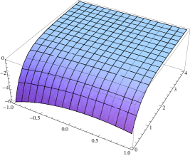
Figure 1: We depict the moduli potential $V(\bar{\tau}\,,~{}\bar{\rho})$ in the type IIA theory for the case of $R({\rm Y})=1$ , $A_{\rm Y}=1$ , $A_{\rm H}=A_{p}=A_{{\rm D}p}=0$ , and $A_{{\rm O}p}\int d^{p-3}x\sqrt{g_{p-3}}=1\,,~{}(p=4,6,8)$ . We also fix $\kappa=1$  [34]. The moduli potential has negative value.

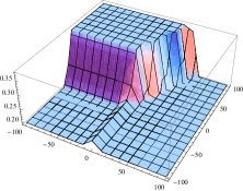
Figure 2: For the case of $R({\rm Y})=1$ , $A_{\rm Y}=1$ , $A_{\rm H}=A_{p}=A_{{\rm D}p}=0$ , and $A_{{\rm O}p}\int d^{p-3}x\sqrt{g_{p-3}}=1\,,~{}(p=4,6,8)$ , in the moduli potential (12) of the type IIA theory, the parameters $\varepsilon_{\rm f}(\bar{\tau}\,,~{}\bar{\rho})$ , $\eta_{\rm f}(\bar{\tau}\,,~{}\bar{\rho})$ , are depicted. We set $\kappa=1$ [34]. Since these results give the contradiction with the fast-roll condition for ekpyrosis (13) , the ekpyrosis is not allowed.

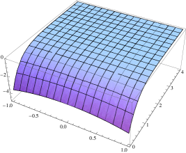
Figure 3: The moduli potential $V(\bar{\tau}\,,~{}\bar{\rho})$ in the type IIA theory for the case of $R({\rm Y})=0$ , $A_{\rm H}=A_{p}=A_{{\rm D}p}=0$ , and $A_{{\rm O}p}\int d^{p-3}x\sqrt{g_{p-3}}=1\,,~{}(p=4,6,8)$ is depicted. Fixing the four-dimensional gravitational constant as $\kappa=1$ , we obtain the negative potential.

Figure 4: We fix $R({\rm Y})=0$ , $A_{\rm H}=A_{p}=A_{{\rm D}p}=0$ , and $A_{{\rm O}p}\int d^{p-3}x\sqrt{g_{p-3}}=1\,,~{}(p=4,6,8)$ , and set $\kappa=1$ . in the moduli potential (12) for the type IIA theory. We depicted the behavior of the parameters $\varepsilon_{\rm f}(\bar{\tau}\,,~{}\bar{\rho})$ , $\eta_{\rm f}(\bar{\tau}\,,~{}\bar{\rho})$ . Our setup cannot describe the ekpyrotic scenario because the background does not obey the fast-roll condition (13).

2.2 Type IIB compactification

There are many no-go theorems and exclude most concrete examples of de Sitter solution [36, 44, 45, 46, 47]. It is possible to evade simple no-go theorems of inflationary scenario for SU(2)$\times$SU(2) with an SU(2)-structure and O5- and O7-planes. Although there are de Sitter critical points, these have at least one tachyonic direction with a large $\eta$ (slow-roll) parameter [47].

On the other hand, for type IIB compactifications in the ekpyrotic model, we have also seen that it is possible to obtain simple no-go theorems in the ($\bar{\rho}$ , $\bar{\tau}$)-plane if one includes orientifold planes and the curvature of the internal space. The behavior of four-dimensional scalar potential is numerically illustrated in Fig. 5 for $R({\rm Y})=1$, and in Fig. 7 for $R({\rm Y})=0$ .

From the Eq. (13), we find a constraint of the fast-roll parameter $\varepsilon_{\rm f}$

$$\varepsilon_{\rm f} = V^{2}\left[2\left\{V_{\rm Y}+\frac{3}{2}\left(V_{\rm O3}+V_{\rm O5}+V_{\rm O7}+V_{\rm O9}\right)\right\}^{2}\right.$$ (16)

$$\left.+\frac{1}{6}\left(2V_{\rm Y}+3V_{\rm O3}+V_{\rm O5}-V_{\rm O7}-3V_{\rm O9}\right)^{2}\right]^{-1}>\frac{1}{6}\,.$$

Unfortunately, the form moduli potential is not steep again as $\varepsilon_{\rm f}$ and $\eta_{\rm f}$ parameters turns out to be large value. Just as in the IIA analogue, one obtains the bound $\varepsilon_{\rm f}>1/6$ . If we choose different values for $A_{\rm Y}$ and $A_{{\rm O}p}$ in the moduli potential (12), we can find again the same bound. We show fast-roll parameters $\varepsilon_{\rm f}$ and $\eta_{\rm f}$ numerically in Fig. 6 (for $R({\rm Y})=1$) and Fig. 8 (for $R({\rm Y})=0$) in the IIB theory.

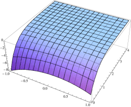
Figure 5: The figure shows the moduli potential $V(\bar{\tau}\,,~{}\bar{\rho})$ in the type IIB theory for the case of $R({\rm Y})=1$ , $A_{\rm Y}=1$ , $A_{\rm H}=A_{p}=A_{{\rm D}p}=0$ , $A_{{\rm O}p}\int d^{p-3}x\sqrt{g_{p-3}}=1\,,~{}(p=3,5,7,9)$ , and $\kappa=1$ . The potential of the moduli becomes negative without flux.

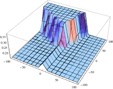
Figure 6: We shows the behavior of parameters $\varepsilon_{\rm f}(\bar{\tau}\,,~{}\bar{\rho})$ , $\eta_{\rm f}(\bar{\tau}\,,~{}\bar{\rho})$ for the type IIB theory. We set $R({\rm Y})=1$ , $A_{\rm Y}=1$ , $A_{\rm H}=A_{p}=A_{{\rm D}p}=0$ , $A_{{\rm O}p}\int d^{p-3}x\sqrt{g_{p-3}}=1\,,~{}(p=3,5,7,9)$ , and $\kappa=1$ , in the moduli potential (12), the parameters $\varepsilon_{\rm f}(\bar{\tau}\,,~{}\bar{\rho})$ , $\eta_{\rm f}(\bar{\tau}\,,~{}\bar{\rho})$ , are depicted. Since these results are not consistent with the fast-roll condition for ekpyrosis (13) , we cannot describe the ekpyrotic scenario in our background.

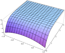
Figure 7: The moduli potential $V(\bar{\tau}\,,~{}\bar{\rho})$ in the type IIB theory for the case of $R({\rm Y})=0$ , $A_{\rm H}=A_{p}=A_{{\rm D}p}=0$ , and $A_{{\rm O}p}\int d^{p-3}x\sqrt{g_{p-3}}=1\,,~{}(p=3,5,7,9)$ , and $\kappa=1$ is shown in the $(\bar{\tau}\,,~{}\bar{\rho})$ space. Although the moduli potential becomes negative, the form of the moduli potential is not steep due to $\varepsilon_{\rm f}>1/6$ ,  (See Fig. 8) . In this setup, we cannot describe the ekpyrotic scenario.

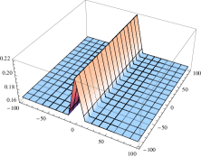
Figure 8: We show the parameters $\varepsilon_{\rm f}(\bar{\tau}\,,~{}\bar{\rho})$ , and $\eta_{\rm f}(\bar{\tau}\,,~{}\bar{\rho})$ , numerically for the type IIB theory. Our parameters are $R({\rm Y})=0$ , $A_{\rm H}=A_{p}=A_{{\rm D}p}=0$ , and $A_{{\rm O}p}\int d^{p-3}x\sqrt{g_{p-3}}=1\,,~{}(p=3,5,7,9)$ , and $\kappa=1$ , in the moduli potential (12). It shows that our setup does not satisfy the fast-roll condition (13).

If we consider the dynamics of remaining moduli such as Kähler moduli, complex structure moduli and axions, the potential is in general a function of hundreds of fields, for large number of infinite families of possible flux combinations on each of the many available internal manifolds. When we treat dynamics of these moduli or the coupling between moduli and fluxes or D-brane, O-plane, they contribute the potential. There is a possibility that the no-go theorems using these fields are circumvented.

3 Discussions

In this note, we have studied the No-Go theorem of the ekpyrosis for string theory in a spacetime of ten dimensions. We gave a potential of the scalar fields in four-dimensional effective theory, in terms of the compactification with smooth manifold.

The effective potential of two scalar fields can be constructed by postulating suitable emergent gravity, orientifold planes, and vanishing fluxes on the ten-dimensional background. The construction of four-dimensional effective action was developed in [34], mainly but not entirely in the context of a new ekpyrotic scenario.

We have used the results of section 2 to analyze the dynamics of moduli that can be constructed using a simple compactification. The scalar potential depends only on two moduli: $\bar{\rho}$ and $\bar{\tau}$ . In such a simple setting, one can show that $\varepsilon_{\rm f}>6/31$ for IIA theory and $\varepsilon_{\rm f}>1/6$ for IIB theory whenever $V(\bar{\rho}\,,\bar{\tau})<0$ . It has been known for some time [4] that the effective potential of scalar fields requires the fast-roll parameter to be small during the ekpyrotic phase. However, with the help of the tools developed in section 2, this is prohibited in a string theory with a compactification. Hence, the explicit nature of the dynamics has made it impossible to realize the ekpyrotic phase in the present note. This is consistent with the results in [43].

As we have commented in Sec. 2 , we have not considered the dynamics for moduli other than the volume modulus of the six-dimensional internal space in this note. If these moduli have dynamics, kinetic terms of moduli appear in the four-dimensional effective theory. Moreover, since moduli couple to orientifolds, it is possible that there are other steep directions of the scalar potential in directions outside the ($\bar{\rho}$ , $\bar{\tau}$)-plane.

The compactification we have considered in this note also gives the No-Go theorem of the inflationary scenario as well as the ekpyrosis because the moduli potential cannot satisfy the slow-roll condition [34]. There are constrains or No-Go theorems to construct the inflationary or de Sitter model in the string theory with a few simple assumptions [34, 42, 48, 49, 50].

In order to embed ekpyrotic or cyclic models in a ten-dimensional supergravity we have investigated in this note, we may consider some ingredients, for instance, the dynamics of remaining moduli, higher curvature correction other than orientifold and flux. We have not attempted an explicit construction here, since that will take us beyond the scope of this note. A lot of study remains to be done in string theory before a cosmologically realistic case is treated.

Appendix A Scalar potential in four-dimensional effective theory

In this appendix, we show how to find the scalar potential in four-dimensional effective theory. We present the explicit procedure for the cases of type II theory with D$p$-brane and O$p$-plane systems.

We assume that ten-dimensional action and metric are given by (1), (2), respectively. We first check the gravity sector. Upon setting the ten-dimensional metric (2), we find

$$\frac{1}{2\bar{\kappa}^{2}}\int d^{10}x\sqrt{-g}\,{\rm e}^{-2\phi}\,R=\frac{1}{2\bar{\kappa}^{2}}\int d^{4}x\sqrt{-q}\,{\rm e}^{-2\phi}\,R\,\rho^{3}\int d^{6}y\sqrt{u}\,,$$ (17)

where $u$ denotes the determinant of the metric $u_{ij}({\rm Y})$ in (2) . We have used the volume modulus of the compact internal space $\rho$ and defined the dilaton modulus $\tau$ by

$$\rho=\left[\frac{\int d^{6}y\sqrt{g_{6}}}{\int d^{6}y\sqrt{u}}\right]^{1/3}\,,~{}~{}~{}~{}~{}\tau={\rm e}^{-\phi}\rho^{3/2}\,,$$ (18)

where $g_{6}$ is the determinant of the metric $g_{ij}$ . In order to obtain the canonical form in the gravity sector, we perform a conformal transformation on the four-dimensional metric to the Einstein frame

$$\bar{q}_{\mu\nu}=\left(\frac{\tau\kappa}{\bar{\kappa}}\right)^{2}q_{\mu\nu}\,,$$ (19)

where $\kappa^{2}$ is the four-dimensional constant and we have chosen a volume modulus $\rho$ such that the metric $u_{ij}({\rm Y})$ of the internal space is normalized $\int d^{6}y\sqrt{u}=1$ . After performing the conformal transformation, the kinetic terms of moduli are given by diagonal form. Since these do not have canonical kinetic energies, we redefine them [34]

$$\bar{\rho}=\sqrt{\frac{3}{2}}\kappa^{-1}\ln\rho\,,~{}~{}~{}~{}~{}\bar{\tau}=\sqrt{{2}}\kappa^{-1}\ln\tau\,.$$ (20)

In terms of fields $\bar{\rho}$ , $\bar{\tau}$ , the gravity sector in the four-dimensional effective action is given by

$$S_{\rm E1} = \int d^{4}x\sqrt{-\bar{q}}\left[\frac{1}{2\kappa^{2}}\bar{R}-\frac{1}{2}\bar{q}^{\mu\nu}\partial_{\mu}\bar{\rho}\partial_{\nu}\bar{\rho}-\frac{1}{2}\bar{q}^{\mu\nu}\partial_{\mu}\bar{\tau}\partial_{\nu}\bar{\tau}\right.$$ (21)

$$~{}~{}~{}~{}~{}\left.+A_{\rm Y}\exp\left\{-\kappa\left(\sqrt{2}\bar{\tau}+\frac{\sqrt{6}}{3}\bar{\rho}\right)\right\}R({\rm Y})\right],$$

where the Ricci scalar $\bar{R}$ , determinant $\bar{q}$ are defined with respect to the metric $\bar{q}_{\mu\nu}$ , $R({\rm Y})$ denotes the Ricci scalar constructed from the metric $u_{ij}({\rm Y})$ , and the coefficient $A_{\rm Y}$ is the function of internal space moduli.

Next we consider contributions of field strengths in the ten-dimensional action (1). We assume that field strengths $H$ and $F_{p}$ can have a non-vanishing integral over any closed three-, $p$-dimensional homology cycle $\Sigma$ , ${\cal C}_{p}$ of the compact space Y, respectively. Since these field strengths satisfy the generalized Dirac charge quantization condition (8), the four-dimensional effective potential includes the appropriate factors of the volume and dilaton from the compactification. The contributions from the field strengths in the four-dimensional Einstein frame action can be expressed as

$$S_{\rm E2} = -\int d^{4}x\sqrt{-\bar{q}}\left[A_{H}\exp\left\{-\kappa\left(\sqrt{2}\bar{\tau}+\sqrt{6}\bar{\rho}\right)\right\}\right.$$ (22)

$$\left.+\sum_{p}A_{p}\exp\left[-\kappa\left\{2\sqrt{2}\bar{\tau}+\frac{\sqrt{6}}{3}(p-3)\bar{\rho}\right\}\right]\right],$$

where coefficients $A_{H}$ and $A_{p}$ depend on the moduli of the internal space.

Finally we consider the four-dimensional effective action coming from D$p$-branes, O$p$-planes term in (1). O$p$-plane is compactified by $(p-3)$-dimensional internal space because they extend our four-dimensional universe. Then, the four-dimensional Einstein frame action arises from the dimensional reduction of the terms in (1) associated with the various D$p$-branes, O$p$-planes becomes

$$S_{\rm E3} = -\int d^{4}x\sqrt{-\bar{q}}\,\sum_{p}\left(A_{{\rm D}p}-A_{{\rm O}p}\right)\exp\left[-\kappa\left\{\frac{3\sqrt{2}}{2}\bar{\tau}+\frac{\sqrt{6}}{6}(6-p)\bar{\rho}\right\}\right]$$ (23)

$$\times\int d^{p-3}x\sqrt{g_{p-3}}\,.$$

From Eqs. (21), (22) and (23), the four-dimensional effective action $S_{\rm E}$ in the Einstein frame is described as

$$S_{\rm E} = S_{\rm E1}+S_{\rm E2}+S_{\rm E3}$$ (24)

$$= \int d^{4}x\sqrt{-\bar{q}}\left[\frac{1}{2\kappa^{2}}\bar{R}-\frac{1}{2}\bar{q}^{\mu\nu}\partial_{\mu}\bar{\rho}\,\partial_{\nu}\bar{\rho}-\frac{1}{2}\bar{q}^{\mu\nu}\partial_{\mu}\bar{\tau}\,\partial_{\nu}\bar{\tau}-V\left(\bar{\tau},\bar{\rho}\right)\right],$$

where $V\left(\bar{\tau},\bar{\rho}\right)$ is the scalar potential [34]:

$$V\left(\bar{\tau},\bar{\rho}\right) = -A_{\rm Y}\exp\left[-\kappa\left(\sqrt{2}\bar{\tau}+\frac{\sqrt{6}}{3}\bar{\rho}\right)\right]R({\rm Y})+A_{H}\exp\left[-\kappa\left(\sqrt{2}\bar{\tau}+\sqrt{6}\bar{\rho}\right)\right]$$ (25)

$$+\sum_{p}A_{p}\exp\left[-\kappa\left\{2\sqrt{2}\bar{\tau}+\frac{\sqrt{6}}{3}(p-3)\bar{\rho}\right\}\right]$$

$$+\sum_{p}\left(A_{{\rm D}p}-A_{{\rm O}p}\right)\exp\left[-\kappa\left\{\frac{3\sqrt{2}}{2}\bar{\tau}+\frac{\sqrt{6}}{6}(p-6)\bar{\rho}\right\}\right]\int d^{p-3}x\sqrt{g_{p-3}}\,.$$

References

- [1] J. Khoury, B. A. Ovrut, P. J. Steinhardt and N. Turok, “The Ekpyrotic universe: Colliding branes and the origin of the hot big bang,” Phys. Rev. D 64 (2001) 123522 [hep-th/0103239].
- [2] P. J. Steinhardt and N. Turok, “A Cyclic model of the universe,” Science 296 (2002) 1436 [hep-th/0111030].
- [3] J. K. Erickson, S. Gratton, P. J. Steinhardt and N. Turok, “Cosmic perturbations through the cyclic ages,” Phys. Rev. D 75 (2007) 123507 [hep-th/0607164].
- [4] J. L. Lehners, “Ekpyrotic and Cyclic Cosmology,” Phys. Rept. 465 (2008) 223 [arXiv:0806.1245 [astro-ph]].
- [5] J. L. Lehners, P. J. Steinhardt and N. Turok, “The Return of the Phoenix Universe,” Int. J. Mod. Phys. D 18 (2009) 2231 [arXiv:0910.0834 [hep-th]].
- [6] J. Khoury and P. J. Steinhardt, “Adiabatic Ekpyrosis: Scale-Invariant Curvature Perturbations from a Single Scalar Field in a Contracting Universe,” Phys. Rev. Lett. 104 (2010) 091301 [arXiv:0910.2230 [hep-th]].
- [7] D. H. Lyth, “The Primordial curvature perturbation in the ekpyrotic universe,” Phys. Lett. B 524 (2002) 1 [hep-ph/0106153].
- [8] R. Brandenberger and F. Finelli, “On the spectrum of fluctuations in an effective field theory of the Ekpyrotic universe,” JHEP 0111 (2001) 056 [hep-th/0109004].
- [9] J. C. Hwang, “Cosmological structure problem in the ekpyrotic scenario,” Phys. Rev. D 65 (2002) 063514 [astro-ph/0109045].
- [10] J. Khoury, B. A. Ovrut, P. J. Steinhardt and N. Turok, “Density perturbations in the ekpyrotic scenario,” Phys. Rev. D 66 (2002) 046005 [hep-th/0109050].
- [11] D. H. Lyth, “The Failure of cosmological perturbation theory in the new ekpyrotic scenario,” Phys. Lett. B 526 (2002) 173 [hep-ph/0110007].
- [12] S. Tsujikawa, “Density perturbations in the ekpyrotic universe and string inspired generalizations,” Phys. Lett. B 526 (2002) 179 [gr-qc/0110124].
- [13] A. Notari and A. Riotto, “Isocurvature perturbations in the ekpyrotic universe,” Nucl. Phys. B 644 (2002) 371 [hep-th/0205019].
- [14] S. Tsujikawa, R. Brandenberger and F. Finelli, “On the construction of nonsingular pre - big bang and ekpyrotic cosmologies and the resulting density perturbations,” Phys. Rev. D 66 (2002) 083513 [hep-th/0207228].
- [15] J. L. Lehners, P. McFadden, N. Turok and P. J. Steinhardt, “Generating ekpyrotic curvature perturbations before the big bang,” Phys. Rev. D 76 (2007) 103501 [hep-th/0702153 [hep-th]].
- [16] E. I. Buchbinder, J. Khoury and B. A. Ovrut, “New Ekpyrotic cosmology,” Phys. Rev. D 76 (2007) 123503 [hep-th/0702154].
- [17] K. Koyama, S. Mizuno and D. Wands, “Curvature perturbations from ekpyrotic collapse with multiple fields,” Class. Quant. Grav. 24 (2007) 3919 [arXiv:0704.1152 [hep-th]].
- [18] K. Koyama, S. Mizuno, F. Vernizzi and D. Wands, “Non-Gaussianities from ekpyrotic collapse with multiple fields,” JCAP 0711 (2007) 024 [arXiv:0708.4321 [hep-th]].
- [19] E. I. Buchbinder, J. Khoury and B. A. Ovrut, “Non-Gaussianities in new ekpyrotic cosmology,” Phys. Rev. Lett. 100 (2008) 171302 [arXiv:0710.5172 [hep-th]].
- [20] J. L. Lehners and P. J. Steinhardt, “Non-Gaussian density fluctuations from entropically generated curvature perturbations in Ekpyrotic models,” Phys. Rev. D 77 (2008) 063533 Erratum: [Phys. Rev. D 79 (2009) 129903] [arXiv:0712.3779 [hep-th]].
- [21] J. L. Lehners and P. J. Steinhardt, “Intuitive understanding of non-gaussianity in ekpyrotic and cyclic models,” Phys. Rev. D 78 (2008) 023506 Erratum: [Phys. Rev. D 79 (2009) 129902]
- [22] S. Mizuno, K. Koyama, F. Vernizzi and D. Wands, “Primordial non-Gaussianities in new ekpyrotic cosmology,” AIP Conf. Proc. 1040 (2008) 121.
- [23] A. Linde, V. Mukhanov and A. Vikman, “On adiabatic perturbations in the ekpyrotic scenario,” JCAP 1002 (2010) 006 [arXiv:0912.0944 [hep-th]].
- [24] J. L. Lehners, “Ekpyrotic Non-Gaussianity: A Review,” Adv. Astron. 2010 (2010) 903907 [arXiv:1001.3125 [hep-th]].
- [25] M. Li, “Note on the production of scale-invariant entropy perturbation in the Ekpyrotic universe,” Phys. Lett. B 724 (2013) 192 [arXiv:1306.0191 [hep-th]].
- [26] L. Battarra and J. L. Lehners, “Quantum-to-classical transition for ekpyrotic perturbations,” Phys. Rev. D 89 (2014) no.6, 063516 [arXiv:1309.2281 [hep-th]].
- [27] A. Fertig, J. L. Lehners and E. Mallwitz, “Ekpyrotic Perturbations With Small Non-Gaussian Corrections,” Phys. Rev. D 89 (2014) no.10, 103537 [arXiv:1310.8133 [hep-th]].
- [28] A. Ijjas, J. L. Lehners and P. J. Steinhardt, “General mechanism for producing scale-invariant perturbations and small non-Gaussianity in ekpyrotic models,” Phys. Rev. D 89 (2014) no.12, 123520 [arXiv:1404.1265 [astro-ph.CO]].
- [29] A. M. Levy, A. Ijjas and P. J. Steinhardt, “Scale-invariant perturbations in ekpyrotic cosmologies without fine-tuning of initial conditions,” Phys. Rev. D 92 (2015) no.6, 063524 [arXiv:1506.01011 [astro-ph.CO]].
- [30] A. Fertig and J. L. Lehners, “The Non-Minimal Ekpyrotic Trispectrum,” JCAP 1601 (2016) no.01, 026 [arXiv:1510.03439 [hep-th]].
- [31] A. Ito and J. Soda, “Primordial Gravitational Waves Induced by Magnetic Fields in an Ekpyrotic Scenario,” Phys. Lett. B 771 (2017) 415 [arXiv:1607.07062 [hep-th]].
- [32] S. Gratton, J. Khoury, P. J. Steinhardt and N. Turok, “Conditions for generating scale-invariant density perturbations,” Phys. Rev. D 69 (2004) 103505 [astro-ph/0301395].
- [33] J. Khoury, P. J. Steinhardt and N. Turok, Designing cyclic universe models,” Phys. Rev. Lett. 92 (2004) 031302 [hep-th/0307132].
- [34] M. P. Hertzberg, S. Kachru, W. Taylor and M. Tegmark, “Inflationary Constraints on Type IIA String Theory,” JHEP 0712 (2007) 095 [arXiv:0711.2512 [hep-th]].
- [35] S. S. Haque, G. Shiu, B. Underwood and T. Van Riet, “Minimal simple de Sitter solutions,” Phys. Rev. D 79 (2009) 086005 [arXiv:0810.5328 [hep-th]].
- [36] S. B. Giddings, S. Kachru and J. Polchinski, “Hierarchies from fluxes in string compactifications,” Phys. Rev. D 66 (2002) 106006 [hep-th/0105097].
- [37] S. Kachru, R. Kallosh, A. D. Linde and S. P. Trivedi, “De Sitter vacua in string theory,” Phys. Rev. D 68 (2003) 046005 [hep-th/0301240].
- [38] G. Villadoro and F. Zwirner, “ effective potential from dual type-IIA D6/O6 orientifolds with general fluxes,” JHEP 0506 (2005) 047 [hep-th/0503169].
- [39] O. DeWolfe, A. Giryavets, S. Kachru and W. Taylor, “Type IIA moduli stabilization,” JHEP 0507 (2005) 066 [hep-th/0505160].
- [40] B. de Carlos, A. Guarino and J. M. Moreno, “Flux moduli stabilisation, Supergravity algebras and no-go theorems,” JHEP 1001 (2010) 012 [arXiv:0907.5580 [hep-th]].
- [41] E. Silverstein, “Simple de Sitter Solutions,” Phys. Rev. D 77 (2008) 106006 [arXiv:0712.1196 [hep-th]].
- [42] U. H. Danielsson, S. S. Haque, G. Shiu and T. Van Riet, “Towards Classical de Sitter Solutions in String Theory,” JHEP 0909 (2009) 114 [arXiv:0907.2041 [hep-th]].
- [43] Eline Meeus, “A nogo-theorem for Ekpyrosis from 10D supergravity,” master’s thesis, KU Leuven (2016).
- [44] G. W. Gibbons, “Aspects Of Supergravity Theories,” Print-85-0061 (CAMBRIDGE).
- [45] B. de Wit, D. J. Smit and N. D. Hari Dass, “Residual Supersymmetry of Compactified Supergravity,” Nucl. Phys. B 283 (1987) 165.
- [46] J. M. Maldacena and C. Nunez, “Supergravity description of field theories on curved manifolds and a no go theorem,” Int. J. Mod. Phys. A 16 (2001) 822 [hep-th/0007018].
- [47] C. Caviezel, T. Wrase and M. Zagermann, “Moduli Stabilization and Cosmology of Type IIB on SU(2)-Structure Orientifolds,” JHEP 1004 (2010) 011 [arXiv:0912.3287 [hep-th]].
- [48] T. Wrase and M. Zagermann, “On Classical de Sitter Vacua in String Theory,” Fortsch. Phys. 58 (2010) 906 [arXiv:1003.0029 [hep-th]].
- [49] G. Shiu and Y. Sumitomo, “Stability Constraints on Classical de Sitter Vacua,” JHEP 1109 (2011) 052 [arXiv:1107.2925 [hep-th]].
- [50] T. Van Riet, “On classical de Sitter solutions in higher dimensions,” Class. Quant. Grav. 29 (2012) 055001 [arXiv:1111.3154 [hep-th]].