A Modeling Framework for Schedulability Analysis of Distributed Avionics Systems

Abstract

This paper presents a modeling framework for schedulability analysis of distributed integrated modular avionics (DIMA) systems that consist of spatially distributed ARINC-653 modules connected by a unified AFDX network. We model a DIMA system as a set of stopwatch automata (SWA) in Uppaal to analyze its schedulability by classical model checking (MC) and statistical model checking (SMC). The framework has been designed to enable three types of analysis: global SMC, global MC, and compositional MC. This allows an effective methodology including (1) quick schedulability falsification using global SMC analysis, (2) direct schedulability proofs using global MC analysis in simple cases, and (3) strict schedulability proofs using compositional MC analysis for larger state space. The framework is applied to the analysis of a concrete DIMA system.

1 Introduction

In the avionics industry, Distributed Integrated Modular Avionics (DIMA) has been widely recognized as a promising architecture and the next generation of Integrated Modular Avionics (IMA). A DIMA system installs standardized IMA modules in spatially distributed processors[16] that communicate through a unified bus system[5] such as an AFDX network. Avionics functions residing on the IMA modules are implemented in the form of application software running in an ARINC-653[3] compliant operating system. The generic distributed structure of DIMA significantly improves performance and reliability as well as lowers weight and cost, while it also dramatically increases the complexity of schedulability analysis. A schedulable DIMA system should fulfil not only the temporal requirements of real-time tasks in each ARINC-653 module but also several communication constraints among the distributed nodes. As a result, the DIMA architecture requires the system integrators to analyze schedulability considering both computation and communication.

The development of model checking based approaches has currently become an attractive topic for the schedulability analysis of complex real-time systems due to the sufficient expressiveness of formal models. The techniques of classical model checking (MC) describe schedulability as temporal logic properties and verify the properties via symbolic state space exploration. Unfortunately, when being applied to a complete avionics system, all of them suffer from an inevitable problem of state space explosion, which makes the exact symbolic model checking practically infeasible.

Accordingly, Statistical Model Checking (SMC) is proposed as a promising technique that has powerful facilities of formal modeling as well as avoids the state-space explosion of classical model checking. A SMC engine runs and monitors a number of simulation processes, quickly estimating the statistical results of the satisfaction or violation of certain properties. However, SMC cannot provide any guarantee of schedulability but quick falsification owing to its nature of statistical testing. Therefore, it is reasonable to apply both classical and statistical model checking to the schedulability analysis of avionics systems.

Related work: We found no studies that analyzed the schedulability of distributed avionics systems as a whole including the network by model checking. The related research isolates computation modules from their underlying network, thereby considering these nodes as independent hierarchical scheduling systems or investigating the network in isolation, which possibly leads to pessimistic results. There have been works using model-checking approaches to analyze the temporal behavior of individual avionics modules in various formal models such as Coloured Petri Nets (CPN)[12], preemptive Time Petri Nets (pTPN)[7], Timed Automata (TA)[4], and StopWatch Automata (SWA)[10], and verify schedulability properties via state space exploration. For hierarchical scheduling systems, some studies[8, 15, 6] exploit the inherent temporal isolation of ARINC-653 partitions[3] and analyze each partition separately, but they ignore the behavior of the underlying network or the interactions among partitions. Thus these methods are not applicable to DIMA environments in which multiple distributed ARINC-653 partitions communicate through a shared network to perform an avionics function together.

Contributions: In this paper, we present a modeling framework for schedulability analysis of DIMA systems that are implemented as a set of Uppaal SWA, i.e. the TA extended with stopwatches[9] in Uppaal. The framework combines compositional and global analysis by classical and statistical model checking. The main contributions of this paper are summarized as follows:

• Modeling of DIMA systems covers the major behavior of two-level ARINC-653 compliant schedulers, periodic/sporadic tasks, intra-partition synchronization, and inter-partition communications through an AFDX network.

• Compositional analysis using classical model checking verifies the model of each ARINC-653 partition including its environment individually and then assemble the local results together to derive conclusions about the schedulability of an entire system.

• Global analysis using statistical model checking allows users to quickly falsify non-schedulable configurations by SMC hypothesis testing, which can handle a complete system model and avoid an exhaustive exploration of the state space.

The rest of the paper is organized as follows. Section 2 describes the structure of a DIMA system. An overview of the modeling framework is presented in section 3, where the methods of compositional and global analysis are briefly outlined. In section 4, we detail the Uppaal models of the framework. Section 5 shows an experiment on a concrete DIMA system, and section 6 finally concludes.

2 Avionics System Description

We consider a generic architecture of a DIMA system with several ARINC-653 modules connected by an AFDX network shown in Fig.2. There is a three-layer structure in the DIMA architecture consisting of scheduling, task, and communication layers.

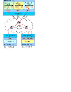
Figure 1: An Example of DIMA systems

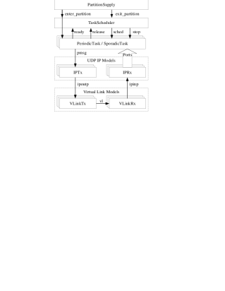
Figure 2: An Overview of Modeling Framework

The scheduling layer comprises the scheduling facilities for generic computation resources in a DIMA system, where physically distributed modules with independent computational power execute application tasks simultaneously. The tasks run in a partitioned operating system which provides a two-level scheduling mechanism and achieves temporal isolation between ARINC-653 partitions. In such a scheduling system, partitions are scheduled by a Time Division Multiplexing (TDM) scheduler and each partition also has its local scheduling policy, preemptive Fixed Priority (FP), to handle the internal tasks[3].

All the application tasks executing avionics functions constitute the task layer. We consider a task as the smallest scheduling unit, each of which can be executed concurrently with other tasks in the same partition. Assume that jobs of each task are scheduled repeatedly. We define two task types: periodic tasks and sporadic tasks. A periodic task has a fixed release period, while a sporadic task is characterized by a minimum separation between consecutive jobs.

The communication layer provides the services of inter-partition communication over a common AFDX network. The AFDX protocol stack realized by an End System(ES) interfaces with the task layer through ARINC-653 ports. Based on the AFDX protocol structure, the communication layer is further divided into UDP/IP layer and Virtual Link layer, where a Virtual Link (VL) ensures an upper bound on end-to-end delay.

The communication layer also affects the schedulability of the system. According to the ARINC-653 standard[3], there are two types of ARINC-653 ports, sampling ports and queuing ports. A sampling port can accommodate at most a single message that remains until it is overwritten by a new message. Moreover, a refresh period is defined for each sampling port. This attribute provides a specified arrival rate of messages, regardless of the rate of read requests from tasks. In contrast, a queuing port is allowed to buffer multiple messages in a message queue with a fixed capacity. However, the operating system is not responsible for handling overflow from the message queue.

In our framework, we verify the three following schedulability properties of DIMA systems: (1) All the tasks meet their deadlines in each partition. (2) The refresh period of any sampling port is guaranteed. (3) The overflow from any queuing ports is avoided.

3 An Overview of the Modeling Framework

3.1 An Outline of the UPPAAL Models

The Uppaal templates in the modeling framework are organized as the above layered structure. Fig.2 shows an overview of these templates together with the channels between them.

The scheduling layer consists of two TA templates PartitionScheduler and TaskScheduler. The PartitionScheduler model provides the service of TDM partition scheduler for any partition. The Tas-
kScheduler model implementing FP scheduling policy allocates processor time to the task layer only when the partition is active. Hence PartitionScheduler sends notification on the broadcast channels enter_partition and exit_partition to TaskScheduler when entering and leaving its partition, respectively.

The task layer contains a set of task models which are instantiated from two SWA templates Periodi-
cTask and SporadicTask. A task model describes an instance of an avionics program. Since the tasks in a partition are scheduled by a task scheduler, we define four channels ready, release, sched and stop as a set of scheduling commands to communicate between task templates and TaskScheduler. Moreover, the priority ceiling protocol is implemented by mutexes in task models to deal with intra-partition synchronization.

The communication layer comprises two types of models: UDP/IP and VL models. The UDP/IP models are divided into two TA templates IPTx and IPRx, which calculate the delivery latency of the UDP/IP layer in a transmitting ES and a receiving ES respectively. When sending a message to an ARINC-653 port, the source task notifies the destination IPTx via the broadcast channel pmsg. In the link layer, two TA templates VLinkTx and VLinkRx model the total latency of a VL through the transmitting ES and the reception network respectively. The channel vl connects VLinkTx and VLinkRx in the same VL. Additionally, there are also two broadcast channels ipoutp and ipinp between the UDP/IP and VL models in opposite directions.

3.2 Integration of MC and SMC

In Uppaal SMC, a model comprises networks of Stochastic Timed Automata (STA), which is designed as a stochastic interpretation and extension of the TA formalism of Uppaal classic[11]. To integrate SMC into a common framework, we adapt the above templates for STA with the following features:

• Input-enabledness: Only broadcast channels, which can attach to an arbitrary number of receivers, do we use in the modeling framework to ensure the input-enabled property that no input actions are prevented from being sent to a STA.

• Deterministic bounded delays: The semantics of non-deterministic delays in TA is replaced with probability distributions. The bounded delay at a location of templates is defined as a uniform distribution in STA. For example, PeriodicTask executes computing operations at a location Running with a bounded delay interval $[\mathit{bcet},\mathit{wcet}]$. Thus we assume this execution time to be random samples from the uniform distribution $U(\mathit{bcet},\mathit{wcet})$.

• Deterministic unbounded delays: The unbounded delays are interpreted as exponential distributions in STA. We take the model SporadicTask for example. There is a minimum separation but no maximum constraint between consecutive releases of a sporadic task. We describe this unbounded separation as an exponential distribution with an empirical rate at a location WaitNextRelease.

• Non-zenoness: We adopt two modeling principles to reduce the risk of zenoness in Uppaal: (1) Avoid the loops composed of permanently enabled edges and urgent/committed locations where time cannot progress. (2) Provide normal locations with two types of outgoing edges, which are either event-driven edges that contain input channels or time-driven edges that do not have input labels but guards making time progress at source locations. Since Uppaal SMC can detect zeno runs[11], the modeling framework has been checked thoroughly to achieve non-zenoness.

3.3 Schedulability Analysis by MC and SMC

On the basis of the above models, we introduce the procedure for our schedulability analysis, which combines classical and statistical model checking together. Fig.3 shows the four steps in the procedure: (1) Scheduling configuration is encoded into the Uppaal model as a structure array. (2) We perform hypothesis testing of SMC for the model to falsify non-schedulable configuration rapidly. (3) If the model goes through the SMC test, its schedulability should be verified by classical symbolic MC. (4) We refine the configuration that fails steps (2,3) and restart step (1).

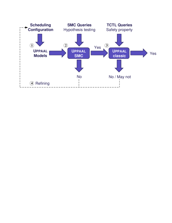
Figure 3: The Procedure for Schedulability Analysis

When we apply classical MC to the analysis of a DIMA system, the schedulability constraints are expressed and verified as a safety property of SWA models. We add a boolean variable error with the initial value False to Uppaal templates for this purpose. Once the schedulability is violated, the related model will assign the value True to error immediately. Thus, the schedulability is replaced with this safety property $\varphi$:

$${{\leavevmode\lstinline{{\lst@@@set@language\lst@@@set@numbers\lst@@@set@frame\lst@@@set@rulecolor\lst@@@set@language{\@listingGroup{ltx_lst_identifier}{A}}[]{\@listingGroup{ltx_lst_space}{}}{\@listingGroup{ltx_lst_identifier}{not}}{\@listingGroup{ltx_lst_space}{}}{\@listingGroup{ltx_lst_identifier}{error}}}}}},$$ (1)

which belongs to a simplified subset of TCTL used in Uppaal.

According to the size of state space, we choose either a global or compositional MC analysis. The system models with small size can be handled by the global analysis where the modeling elements of all the partitions in the system are instantiated and checked directly. Nevertheless, most concrete system models have larger state space, thereby making the global analysis infeasible. To reduce the state space in this case, we perform a compositional analysis which check each partition including its environment individually. A set of message interface automata is built to model the environment for a partition.

The schedulability can be obtained from the satisfaction of $\varphi$, i.e. the MC result “Yes” in Fig.3. However, since the symbolic MC of Uppaal for SWA introduces a slight over-approximation[9], we cannot conclude non-schedulability from the MC results “No” or “May not” with certainty. Therefore, we derive non-schedulability from SMC testing rather than from the verification of $\varphi$.

Considering the scalability of SMC, we only use a global analysis in Uppaal SMC. The schedulability of a complete avionics system is described as following queries of hypothesis testing:

$${{\leavevmode\lstinline{{\lst@@@set@language\lst@@@set@numbers\lst@@@set@frame\lst@@@set@rulecolor\lst@@@set@language{\@listingGroup{ltx_lst_identifier}{Pr}}[\textless={\@listingGroup{ltx_lst_space}{}}{\@listingGroup{ltx_lst_identifier}{M}}](\textless\textgreater{\@listingGroup{ltx_lst_space}{}}{\@listingGroup{ltx_lst_identifier}{error}}){\@listingGroup{ltx_lst_space}{}}\textless=}}}}\theta,$$ (2)

where $M$ is the time bound on the simulations and $\theta$ is a very low probability. Since Uppaal SMC approximates the answer using simulation-based tests, we can falsify non-schedulable configuration (i.e. the SMC result “No” in Fig.3) rapidly by finding counter-examples but identify schedulable ones only with high probability ($1-\theta$) (i.e. the SMC result “Yes” in Fig.3). Hence, the configuration that goes through the SMC tests should be validated by symbolic MC to ensure the schedulability of the corresponding system.

4 UPPAAL Models

In this section, we detail the major Uppaal templates according to the layered structure from top down.

4.1 Scheduling Layer Models

PartitionScheduler template In the scheduling layer, a partition is activated only during its partition windows within every major time frame $T_{\_}{mf}$. We build a TA model PartitionScheduler(See Fig.4) to provide the description of temporal resources for a particular partition.

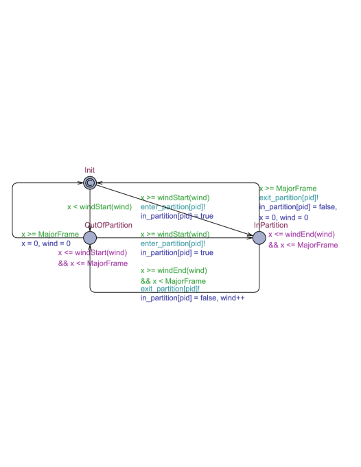
Figure 4: PartitionScheduler Model

The template declarations in Uppaal support the execution of a PartitionScheduler model. The parameter pid of PartitionScheduler is the identifier of its partition and the partition schedule is recorded in an array of structures PartitionWindows. Each element in the array contains two integer fields offset and duration, where offset is the start time of a partition window and duration denotes the duration of this window. By reading PartitionWindowsTable from the declarations, the functions winStart and winEnd with the same integer parameter wind return the start time and the end time of the $wind$th partition window, respectively. The integer constant MajorFrame stands for the major time frame $T_{\_}{mf}$, and the clock x measures time within every $T_{\_}{mf}$. In the template, all the guards and invariants use x to control the transitions between locations.

There are three locations in a PartitionScheduler model. The initial location Init represents a conditional control structure that determines the next location at the start of a major time frame. If a partition window and the major time frame start simultaneously, the model will move to the location InPartition. Otherwise, it will enter the location OutOfPartition. Within a major time frame, the model keeps traveling between InPartition and OutOfPartition according to whether or not the current time is in a partition window. For any time from the initial instant, if the PartitionScheduler model of pid enters a new partition window, it will move to the location InPartition, and notify the unique task scheduler model in pid through the output channel enter_partition. On the contrary, if the PartitionScheduler leaves its current partition window, it will move to the location OutOfPartition, and send notification to the task scheduler model through the output channel exit_partition.

TaskScheduler template For any partition, there is a task scheduler that executes the preemptive FP scheduling policy while the partition is active. The behavior of the task scheduler is depicted in the TA template TaskScheduler (See Fig.5). The only template parameter pid is the identifier of the task scheduler’s partition.

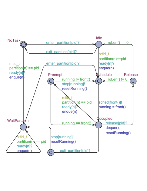
Figure 5: TaskScheduler Model

The model of TaskScheduler receives notification from the PartitionScheduler model through two channels enter_partition and exit_partition, and uses the channels ready, release, sched and stop as scheduling commands to manage the tasks in the partition pid. If there is a task becoming ready to run or relinquishing the processor, the task model will send its TaskScheduler model a ready or release command respectively. TaskScheduler maintains a ready queue that keeps all the tasks ready and waiting to run, and always allocates the processor to the first task with the highest priority in the ready queue. If a new task having a higher priority than any tasks in the ready queue is ready, TaskScheduler will insert the task into the ready queue, interrupt the currently running task via the channel stop and schedule the new selected task via the channel sched. The task identifier is delivered by the offset of channel arrays in the synchronization between TaskScheduler and the task layer.

The ready queue is implemented by the integer array rq which contains a sorted set of task identifiers in priority order. The tasks with identical priority are served in order of readiness. The function rqLen returns the number of the tasks in rq. We use the function enque to insert a new task (identifier) into the ready queue rq and reorder the tasks in the queue. The function deque removes the first element from the ready queue. The first element in rq, namely the identifier of the currently running task, is returned from the function front and recorded in the integer variable running.

Table 1: The Major Locations in Task Scheduler

Location	Partition Windows		Ready Tasks
	Outside	Inside	$\ \ \ 0\ \ \$	$>0$
NoTask	$\surd$		$\surd$
Idle		$\surd$	$\surd$
WaitPartition	$\surd$			$\surd$
Occupied		$\surd$		$\surd$

According to whether the current time is in the partition windows as well as to the number of the tasks in the ready queue, we create four major locations listed in Table 1. These four locations cover all situations, where the model must be at one of these locations for any time from the initial instant. In contrast, all the other locations of the template are committed and utilized to realize conditional branches or atomic action sequences.

4.2 Task Layer Models

We build two SWA templates PeriodicTask and SporadicTask in Uppaal. Both templates share the same skeleton. So we take PeriodicTask for example to sketch out the structure of a task model.

In the template, we define two normal clock x and curTime and a stopwatch exeTime. The clock x measures the delays prescribed by the task type to calculate the release points of the task. The clock curTime is used to determine the start of the next task period. By contrast, the stopwatch exeTime measures the processing time during the execution of an abstract instruction that describes concrete task behavior, and thus progresses only when the model is at the location Running.

Once the task is scheduled by TaskScheduler through the channel sched, it will start execution on the processor and move from the location Ready to ReadOp. For any task in the system, a sequential list of abstract instructions is implemented as the structure array op. By using an integer variable pc as a program counter, the task can fetch the next abstract instruction from op[pc] at the location ReadOp (See Fig.6).

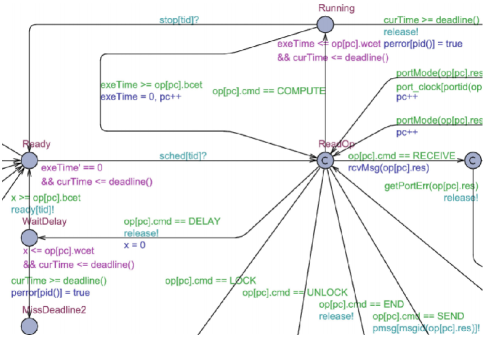
Figure 6: The Main Structure of a Task Model

According to the command in the abstract instruction currently read from op, the task model performs a conditional branch and moves from the location ReadOp to one of the different locations that represent different operations. Therefore, the command set containing the following seven elements divides the rest of the template into seven corresponding parts.

• COMPUTE Command: When the model reads a COMPUTE command, it will (re)start the stopwatch exeTime and enter the location Running, which means that the processor is being occupied by the task and executing a computation instruction.

• LOCK Command: By reading a LOCK command, the task model attempts to acquire the mutual exclusion lock that is specified by the res field of the instruction. The availability of a mutual exclusion lock depend on the priority ceiling protocol.

• UNLOCK Command: When fetching an UNLOCK command from op, the task releases the lock in the instruction and wakes up all the tasks blocked on this lock.

• DELAY Command: The instruction with a DELAY command can make a task suspended at the location WaitDelay for a specified period of time.

• SEND and RECEIVE Command: The commands SEND and RECEIVE represent non-blocking message I/O operations among different partitions.

• END Command: The command END denotes the accomplishment of the current job in this task period. The task will relinquish the processor through the channel release and stay at the location WaitNextRelease until the next period starts.

4.3 Communication Layer Models

The communication layer consists of four templates: IPTx and IPRx calculate the delivery latency of the UDP/IP layer. VLinkTx and VLinkRx calculate the transit delay of frames through a specified VL. We take VLinkTx for example. It calculates the latency of frame delivery through the source ES.

VLinkTx has a template parameter vlid that is the unique identifier of a VL. The VL models read the configuration from the array vlink, which contains a source FIFO buffer src, an array dst of destination FIFO buffers, an identifier es of the VL’s source ES, an integer field BAG that stands for the Bandwidth Allocation Gap (BAG)[2], and an integer field TxDelay denoting the frame delay[2].

The total delay through a VL is divided into technological latency and configuration latency. The technological latency is independent of traffic load, whereas the configuration latency depends on system configuration and traffic load.

We declare two integer constants TechMin and TechMax to be the interval of the technological latency ${{[{\leavevmode\lstinline{{\lst@@@set@language\lst@@@set@numbers\lst@@@set@frame\lst@@@set@rulecolor\lst@@@set@language{\@listingGroup{ltx_lst_identifier}{TechMin}}}}}},{\leavevmode\lstinline{{\lst@@@set@language\lst@@@set@numbers\lst@@@set@frame\lst@@@set@rulecolor\lst@@@set@language{\@listingGroup{ltx_lst_identifier}{TechMax}}}}}}]$. The configuration latency is divided into three parts: the fixed frame delay, the floating delay in waiting for the interval of BAG, and the varying configuration jitter within each BAG. According to the ARINC-664 Part 7[2], a VL should regulate its traffic to send no more than one frame in each BAG. A clock t measures the interval of the jitter as well as the BAG. By contrast, the configuration jitter within BAGs is caused by the interference from the frames of the other VLs in the same transmitting ES[2]. We define an integer array txjitter where each element provides the maximum configuration jitter according to the current traffic at the output of an ES.

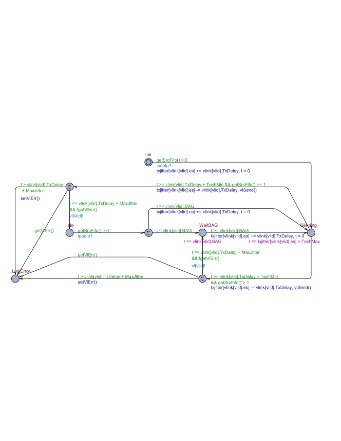
Figure 7: The VLinkTx Model

As is depicted in Fig.7, VLinkTx obtains notification of packet-receiving on the input channel ipoutp. At the initial location Init, VLinkTx waits for the first packet to arrive at the source FIFO. On receiving this first packet, the model enters the location Sending and resets the clock t to start the latency calculation as well as a new BAG interval. Leaving the location Sending means the model completes the sending operation of a frame. At this point, VLinkTx must invoke the function vlSend to decrease the message counter of the source FIFO.

According to the number of packets in the source FIFO, VLinkTx waits for the next BAG interval or the next incoming packet after completing a sending operation. First, if the model still has at least one packet in the source FIFO to transmit, it will enter the location WaitBAG, thereby waiting for the start of the next BAG. Second, if there is only the sent packet in the source FIFO, the model will stay at the location Idle until the arrival of the next incoming packet.

5 Case Study

This section demonstrates the schedulability analysis of an avionics system which combines the workload of [8] and the AFDX configuration of [14]. The workload is comprised of 5 partitions, and further divided into 18 periodic tasks and 4 sporadic tasks. Considering the inter-partition messages in the workload, we assign each message type $\mathit{Msg_{\_}i},i=\{1,2,3,4\}$ a separate VL with the same subscript. The messages of $\mathit{Msg_{\_}1}$ and $\mathit{Msg_{\_}2}$ are handled at the refresh period $50ms$ in sampling ports. $\mathit{Msg_{\_}3}$ and $\mathit{Msg_{\_}4}$ are configured to operate in queuing ports, each of which can accommodate a maximum of one message.

Fig.8 illustrates the distributed deployment of the workload. We consider 3 ARINC-653 modules connected by an AFDX network, and allocate each partition to one of the modules. The module $M_{\_}1$ accommodates $P_{\_}1$ and $P_{\_}2$, the module $M_{\_}2$ executes $P_{\_}3$ and $P_{\_}5$, and the partition $P_{\_}4$ is allocated to $M_{\_}3$. There are 4 VLs $V_{\_}1$-$V_{\_}4$ connecting 3 ESs across 2 switches $S_{\_}1$ and $S_{\_}2$ in the AFDX network. The arrows above VLs’ names indicate the direction of message flow.

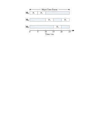
Figure 8: The Distributed Avionics Deployment and Partition Schedules (Times in Milliseconds)

The avionics system equips each of its processor cores with a partition schedule. Assume the modules in the experiment to be single-processor platforms. Fig.8 gives the partition schedules, which fix a common major time frame $T_{\_}{mf}$ at $25ms$ and allocate $5ms$ to each partition within every $T_{\_}{mf}$. All the partition schedules are enabled at the same initial instant and their clocks are always synchronized. The scheduling configuration keeps the temporal order of the partitions in [8]. Hence the partition schedules contain five disjoint windows $\langle P_{\_}1,0,5\rangle$, $\langle P_{\_}2,5,5\rangle$, $\langle P_{\_}3,10,5\rangle$, $\langle P_{\_}4,15,5\rangle$, and $\langle P_{\_}5,20,5\rangle$, where the second parameter is the offset from the start of $T_{\_}{mf}$ and last the duration.

After combining all the models of the system, we executed the schedulability analysis in Uppaal. We set $M=100000$ and $\theta=0.001$ for Eq.(2). The experiment was performed on the Uppaal 4.1.19 64-bit version and an Intel Core i7-5600U laptop processor.

Results of the Analysis

The result (The case 1 in Table 2) shows that the above scheduling configuration fails the SMC test and thus is non-schedulable. We can explore the cause of non-schedulability on the basis of counter-examples to help refine the system configuration.

The Gantt chart in Fig.9 shows such a counter-example, where the task $\mathit{Tsk^{3}_{\_}2}$ in $P_{\_}3$ violates the constraint of the refresh period of $\mathit{Msg_{\_}2}$. At the top of the chart are task models, where the line is painted in green whenever a task stays at Ready state and in blue at Running. The bottom line labels “partition” and “tscheduler” represent two scheduling-layer models PartitionScheduler and TaskScheduler respectively. For the line “partition”, color red denotes the time outside $P_{\_}3$, and green is within $P_{\_}3$. The communication-layer models transmitting the messages of $Msg_{\_}\emph{k}$ correspond to the chart lines “msgk_snd”, “iptxk”, “iprxk”, “vltxk”, and “vlrxk”, which denote the message-delivery delays of $Msg_{\_}\emph{k}$.

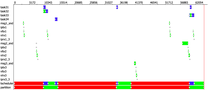
Figure 9: The Gantt Chart of a Counter-example (Times in Microseconds)

The counter-example illustrates that network latency increases the risk of breaching the schedulability constraints. Let $t$ be the elapsed time since the initial instant $t_{\_}0=0$ shown in the Gantt chart. The first message of $\mathit{Msg_{\_}2}$ was sent by the message interface msg2_snd at $t=7.625$ms, and reached the destination port at $t=8.088$ms. When $\mathit{Tsk^{3}_{\_}2}$ was scheduled to read $\mathit{Msg_{\_}2}$ at $t=60.000$ms, the age of the first received message indicated the value $51.912$ms that had exceeded the refresh period. Thus, the copied message of $\mathit{Msg_{\_}2}$ was not a valid data sample. Although msg2_snd sent a new $\mathit{Msg_{\_}2}$ message at $t=59.585$ms, the message did not arrive at the destination port until $t=60.184$ms due to network latency.

Considering the effect of network latency on the scheduling configuration, we updated the partition schedules by performing a swap of time slots between $P_{\_}1$ and $P_{\_}2$. The modified partition schedules provide five windows $\langle P_{\_}1,5,5\rangle$, $\langle P_{\_}2,0,5\rangle$, $\langle P_{\_}3,10,5\rangle$, $\langle P_{\_}4,15,5\rangle$, and $\langle P_{\_}5,20,5\rangle$. The schedulability analysis of the updated system was executed again. The result (The case 2 in Table 2) shows that the configuration goes through the global SMC test and compositional verification of classical MC. Thus, the updated system finally achieves schedulability.

Table 2 shows the execution time and memory usage. In compositional analysis (MC in Table 2), the partition $P_{\_}3$ contains more instantiated models (19 processes) than the other four partitions. As a result, model-checking runs slower and requires more memory than the others. Nevertheless, the compositional analysis could be performed on ordinary computers within an acceptable time.

Compared with the compositional way, global analysis based on the same Uppaal models would require 51 processes including all the 22 task models whose state space is much more complex than the others. This causes Uppaal classic to run out of memory within a few minutes, and thus makes the global analysis using classical MC infeasible. In contrast, SMC testing can be quickly accomplished when we perform global analysis (SMC in Table 2), offering effective state space reduction.

6 Conclusion

In this paper, we present a modeling framework for schedulability analysis of DIMA systems, which are implemented as a set of stopwatch automata in Uppaal. We analyze the Uppaal models including computation and communication by both classical and statistical model checking. The techniques presented in this paper are applicable to the design of DIMA scheduling systems. The experimental results show the applicability of our modeling framework. As future work, we plan to develop a model-based approach to the automatic optimization and generation of a DIMA scheduling system.

Table 2: The Experiment Results (Result), Execution Time (Time/sec.) and Memory Usage (Mem/MB)

Case 1							Case 2
MC				SMC			MC				SMC
No.	Result	Time	Mem	Result	Time	Mem	No.	Result	Time	Mem	Result	Time	Mem
$P_{\_}1$	Yes	7.35	141	No	2.67	53	$P_{\_}1$	Yes	6.07	101	Yes	77.58	53
$P_{\_}2$	Yes	1.02	45				$P_{\_}2$	Yes	1.09	49
$P_{\_}3$	Maynot	57.84	563				$P_{\_}3$	Yes	437.99	3150
$P_{\_}4$	Yes	0.83	45				$P_{\_}4$	Yes	0.88	43
$P_{\_}5$	Yes	33.27	526				$P_{\_}5$	Yes	179.25	2078

Appendix

The appendix consists of three sections. Appendix A gives a description of the remaining Uppaal models in this paper. Appendix B details the avionics workload in the case study. The AFDX configuration is then presented in Appendix C.

Appendix A Remaining Models

A.1 UDP/IP Layer Models

Although the behavior of the UDP/IP layer largely depends on the implementation of the network protocol stack, we create two TA templates IPTx and IPRx to estimate the latency of message delivery through the UDP/IP layer. Both templates have two msgbuf_t parameters src and dst that denote the source buffer and the destination buffer respectively. After being instantiated in the system declarations, these two templates give rise to a set of UDP/IP layer models. By operating the message counters buf in src and dst, the models transfer messages from their respective source buffers to the destination buffers.

Two types of message buffers are provided for the UDP/IP layer models. The first is the port buffers between tasks and the UDP/IP layer. The set of port buffers in the system is defined as a global array portbuf. We declare the second as another global msgbuf_t array fifo which represents the FIFO buffers between the UDP/IP layer and virtual links. Obviously, IPTx and IPRx forward messages in mutually opposed directions.

The template IPTx calculates the latency of message delivery from a port buffer src to a FIFO buffer dst. In order to specify the time interval of forwarding a single message from the source port to the destination FIFO, we declare two integer constants IpFwdMin and IpFwdMax as the lower bound and upper bound, respectively. For any queuing port, the model can perform IP fragmentation according to the integer parameter frag, so breaking one message into $frag$ IP fragments during transmission. In this case, If IPTx handles a message sent from src to dst, the message counter buf of src will be decreased by one, and meanwhile the counter of dst must increase by frag. On the contrary, since sampling ports should not use IP fragmentation[2], the default value 1 is assigned to the template parameters frag of the IPTx models whose source ports are declared to be sampling mode.

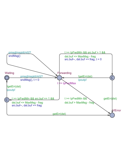
Figure 10: The IPTx Model

As is depicted in Fig.10, an iteration structure realizes the major function of IPTx. After starting from the initial location Waiting, the model keeps waiting for the first incoming message to arrive in the port buffer src. Once any tasks send the port a message through the channel pmsg, IPTx will increase the counter of src by invoking the function sndMsg and thereupon move to the location Forwarding. This location represents that the UDP/IP layer is executing the forwarding operation. Thus, the model can non-deterministically choose a forwarding delay $T_{\_}F$ from the interval ${{[{\leavevmode\lstinline{{\lst@@@set@language\lst@@@set@numbers\lst@@@set@frame\lst@@@set@rulecolor\lst@@@set@language{\@listingGroup{ltx_lst_identifier}{IpFwdMin}}}}}},{\leavevmode\lstinline{{\lst@@@set@language\lst@@@set@numbers\lst@@@set@frame\lst@@@set@rulecolor\lst@@@set@language{\@listingGroup{ltx_lst_identifier}{IpFwdMax}}}}}}]$ and stay at the location Forwarding for $T_{\_}F$ to forward the first message in the src port. Receiving a new incoming message during forwarding will not affect the delay $T_{\_}F$ but only raise the counter of src once more. When the model completes the current forwarding operation, it will send notification to a VL model through the output channel ipoutp! as well as operate the message counters of src and dst. The forwarding operation continues until the source buffer is empty. In other words, if there is still at least one message in the src port, the model will immediately return to the location Forwarding to forward the next message. Otherwise, the model will move back to the initial location Waiting and restart the iteration to wait for the arrival of the following messages.

The template IPTx has a location VlError that represents the existence of errors in the destination VL. First, if any errors are reported by the VL, the function getErr serving as a guard will return $true$ and the model will stop the forwarding iteration at the location VlError. Second, a shortage of FIFO space will also lead the model to VlError. The FIFO dst, which has a MaxMsg capacity, should accommodate at least $frag$ IP packet(s) during every forwarding operation, unless the guard dst.buf > MaxMsg-frag holds at the location Forwarding.

In addition, once the function sndMsg tries sending a message to a full queuing port, the IPTx model will report an overflow error to the source task, which will thereupon move to an error location MsgErr. In contrast, sampling ports can avoid overflow by overwriting the previous message in the buffer. Hence sndMsg assigns 1 directly to the counter of a sampling port.

The template IPRx calculates the latency of message delivery from a FIFO buffer src to a port buffer dst. As is shown in Fig.11, IPRx also includes a forwarding iteration similar to IPTx, but we insert two following parts into the iteration structure.

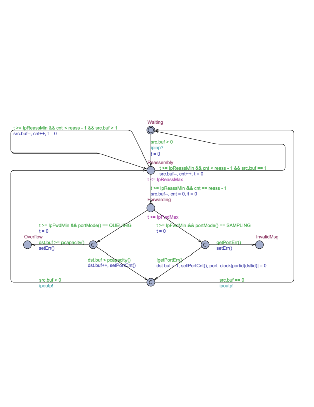
Figure 11: The IPRx Model

The first is a reassembly iteration between the initial location Waiting and the location Forwarding. The nested iteration contains only one Reassembly location, where the model waits for IP packets to arrive and reassembles a complete message. Assume that the IP packets of every message can arrive in order. The template parameter reass denotes that $reass$ consecutive IP packets constitute one complete message. At the location Reassembly, a non-deterministic time between two integer constants IpReassMin and IpReassMax is spent in processing an IP fragment. After this processing delay, the IP packet must be removed from the src FIFO. When reassembling a message, the model uses an integer variable cnt to record the number of IP packets that have arrived of the message. Once the model accumulates the $reass$ consecutive IP packets, it will enter the location Forwarding to forward the complete message to dst.

Second, according to the transfer mode of the destination port dst, we add two different paths following the location Forwarding to operate queuing ports and sampling ports, respectively. For a queuing port, we increase the value of its message counter buf by 1. The guard dst.buf < pcapacity() ensures that the number of messages in dst is less than the capacity of dst. Otherwise, the model will report an overflow error by moving to the Overflow location. For a sampling port, we should fill an empty buffer with the new message or overwrite the previous one. Therefore, IPRx directly assigns 1 to the message counter buf. Meanwhile, IPRx resets the port clock of dst. If a task found an invalid message in the dst after comparing the refresh period of the message with the port clock of the dst, the IPRx model would detect a port error using the function getPortErr and stop its forwarding iteration at the location InvalidMsg.

Both the templatesIPTx and IPRx provide a typical processing procedure for the UDP/IP protocol. Users can easily adapt the templates for their specific implementation.

A.2 Virtual Link Models

We create two TA templates VLinkTx and VLinkRx to calculate the transit delay of frames through a specified VL.

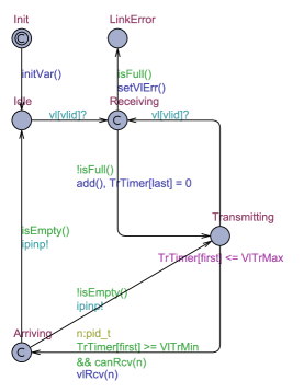
Figure 12: The VLinkRx Model

The template VLinkRx provides the latency of frame delivery through the route from the first switch to a destination ES. In VLinkRx, the integer argument links(resp. switches) denotes the number of physical links(resp. switches) along the route. Assume that each switch and ES can send and receive frames at wire speed. We divide the latency into three parts: the transmission delay of physical links, the processing delay of switches, and the latency at the destination ES. First, given the frame delay vlink[vlid].TxDelay of each physical link, the total transmission delay can be described as the expression $\text{v}\text{l}\text{i}\text{n}\text{k}\text{[}\text{v}\text{l}\text{i}\text{d}\text{]}\text{.}\text{T}\text{x}\text{D}\text{e}\text{l}\text{a}\text{y}\text{∗}\text{l}$

References

- [1]
- [2] AEEC (2009): Aircraft Data Network, Part 7, Avionics Full-Duplex Switched Ethernet Network. ARINC Specification 664P7-1, Aeronautical Radio Inc.
- [3] AEEC (2010): Avionics Application Software Standard Interface: Part 1 - Required Services. ARINC Specification 653P1-3, Aeronautical Radio Inc.
- [4] Tobias Amnell, Elena Fersman, Leonid Mokrushin, Paul Pettersson & Wang Yi: TIMES: a tool for schedulability analysis and code generation of real-time systems. In: FORMATS 2003, 10.1007/978-3-540-40903-86.
- [5] Björn Annighöfer & Frank Thielecke (2014): A Systems Architecting Framework for Distributed Integrated Modular Avionics. DGLR, 10.1007/s13272-015-0156-1.
- [6] Jalil Boudjadar, Kim Guldstrand Larsen, Jin Hyun Kim & Ulrik Nyman: Compositional schedulability analysis of an avionics system using UPPAAL. In: AASE 2014.
- [7] Laura Carnevali, Giuseppe Lipari, Alessandro Pinzuti & Enrico Vicario: A formal approach to design and verification of two-level Hierarchical Scheduling systems. In: RST 2011, 10.1007/BF00360340.
- [8] Laura Carnevali, Alessandro Pinzuti & Enrico Vicario (2013): Compositional verification for hierarchical scheduling of real-time systems. IEEE Transactions on Software Engineering 39(5), pp. 638–657, 10.1109/TSE.2012.54.
- [9] Franck Cassez & Kim Larsen: The impressive power of stopwatches. In: CONCUR 2000, 10.1007/3-540-44618-412.
- [10] Franco Cicirelli, Angelo Furfaro & Libero Nigro et al.: Development of a schedulability analysis framework based on pTPN and UPPAAL with stopwatches. In: DSRA 2012, 10.1109/DS-RT.2012.16.
- [11] Alexandre David, Kim G Larsen, Axel Legay, Marius Mikučionis & Danny Bøgsted Poulsen (2015): Uppaal SMC tutorial. STTT 17(4), pp. 397–415, 10.1007/s10009-014-0361-y.
- [12] RB Dodd (2006): Coloured petri net modelling of a generic avionics mission computer. Technical Report, DTIC.
- [13] Arvind Easwaran, Insup Lee, Oleg Sokolsky & Steve Vestal: A compositional scheduling framework for digital avionics systems. In: RTCSA 2009, 10.1109/RTCSA.2009.46.
- [14] J Javier Gutiérrez, J Carlos Palencia & Michael González Harbour (2014): Holistic schedulability analysis for multipacket messages in AFDX networks. Real-Time Systems 50(2), 10.1007/s11241-013-9192-2.
- [15] Youcheng Sun, Giuseppe Lipari, Romain Soulat, Laurent Fribourg & Nicolas Markey: Component-based analysis of hierarchical scheduling using linear hybrid automata. In: ERCSA 2014, 10.1109/RTCSA.2014.6910502.
- [16] Guoqing Wang & Qingfan Gu: Research on distributed integrated modular avionics system architecture design and implementation. In: DASC 2013, 10.1109/dasc.2013.6712647.