Microscopic vacuum structure in a pure QCD

Abstract

We propose a class of stationary color magnetic solutions in a pure quantum chromodynamics (QCD) which are stable under gluon quantum fluctuations. This resolves a long-standing problem of microscopic description of a stable non-trivial vacuum in a pure QCD. The solutions represent fixed points in a full space of gauge fields under Weyl group transformations. An important feature of the solutions is the phenomenon of Weyl invariant Abelian projection and Abelian dominance in the vacuum structure. As an application of our approach we consider an effective Lagrangian of pure Abelian glueballs in the presence of vacuum gluon condensate.

There is a common belief that the origin of quark and color confinement lies in the vacuum structure which possesses a number of important features. First, the vacuum is formed by means of condensation of some topological defects: monopoles nambu74 ; mandelstam76 ; polyakov77 ; thooft81 , vortices niel-oles ; amb-oles2 ; chernodub14 , center vortices centervort1 ; centervort2 ; centervort3 , dyons diak-petrov etc. A key long-standing problem in such vacuum formation is the quantum instability of the vacuum condensate savv ; N-O . Another important property is an intimate relationship between the gauge invariance of the vacuum and color confinement polyakov77 . At last, the vacuum structure in the confinement phase should admit the ‘t Hooft Abelian projection thooft81 . In this Letter we describe microscopic vacuum structure in a pure QCD which provides the main attributes of a true vacuum.

In perturbative QCD the one particle quantum states (color gluons) do not represent physical observables. To find classical solutions which produce possible physical quantum states after quantization, we follow a guiding principle formulated by H. Weyl: “Whenever you have to do with a structure endowed entity $\Sigma$ try to determine its group of automorphisms… . After that, investigate symmetric configurations of elements which are invariant under a certain subgroup” Weyl1952 . In a case of the group $G=SU(3)$ with a maximal Abelian subgroup $H=U_{3}(1)\times U_{8}(1)$ we look for solutions which are invariant under the Weyl group of outer automorphisms $\{g\in G/H\}$.

We start with a standard $SU(3)$ Yang-Mills type Lagrangian of a pure QCD $(\mu,\nu=0,1,2,3;a=1,...8)$

$${\cal L}_{YM}=-\dfrac{1}{4}F_{\mu\nu}^{a}F^{a\mu\nu},$$ (1)

A generalized axially symmetric Dashen-Hasslacher-Neveu (DHN) ansatz DHN ; plb2018 for non-vanishing components of the gauge potential $A_{\mu}^{a}(r,\theta,t)$ in the holonomic basis reads

$$A_{r}^{2} = K_{1},~{}~{}A_{\theta}^{2}=K_{2},~{}~{}A_{\varphi}^{1}=K_{4},~{}~{}A_{t}^{2}=K_{5},$$

$$A_{r}^{5} = Q_{1},~{}~{}A_{\theta}^{5}=Q_{2},~{}~{}A_{\varphi}^{4}=Q_{4},~{}~{}A_{t}^{5}=Q_{5},$$

$$A_{r}^{7} = S_{1},~{}~{}~{}A_{\theta}^{7}=S_{2},~{}~{}A_{\varphi}^{6}=S_{4},~{}~{}~{}A_{t}^{7}=S_{5},$$ (2)

$$~{}~{}A_{\varphi}^{3}=K_{3},~{}~{}~{}A_{\varphi}^{8}=K_{8},$$

where three sets of gauge fields $K_{i},Q_{i},S_{i}$ $(i=1,2,4,5)$ with proper combinations of the Abelian fields $K_{3,8}$ form the DHN ansatz for each of three $I,U,V$ type subgroups $SU(2)$ neeman99 . To implement the Weyl symmetry we impose additional constraints

$$Q_{1,2,5}=-S_{1,2,5}=-K_{1,2,5},~{}~{}~{}K_{3,8}=-\frac{\sqrt{3}}{2}K_{4},$$

$$Q_{4}=\big{(}-\frac{1}{2}+\frac{\sqrt{3}}{2}\big{)}K_{4},~{}~{}~{}S_{4}=\big{(}-\frac{1}{2}-\frac{\sqrt{3}}{2}\big{)}K_{4}.$$ (3)

The full ansatz (2, 3) is consistent with the original Yang-Mills equations of motion and leads to four second order differential equations and one constraint SM2 which admit a wide class of regular stationary solutions. A special non-Abelian solution with a finite energy density has been found recently in plb2018 ; SM2 . We describe a general class of regular solutions of non-Abelian and Abelian type with a definite parity under the space reflection $\theta\rightarrow\pi-\theta$. In the leading order of Fourier series decomposition the solutions are well approximated by the following factorized form with the numeric accuracy 1.5% (the source of such a high accuracy is explained in plb2018 )

$$K_{1,2,4}(r,\theta,t) = \tilde{K}_{1,2,4}(Mr,\theta)\cos(Mt),$$

$$K_{5}(r,\theta,t) = \tilde{K}_{5}(Mr,\theta)\sin(Mt),$$ (4)

where $M$ is a conformal mass scale parameter. A new solution with the lowest non-trivial polar angle modes is shown in Fig. 1a-d (numeric details are given in SM2 ). The solution differs from the one obtianed in plb2018 by an opposite parity of the fields $K_{1,2,5}$,

(a)  

(b)  

(c)  

(d)  

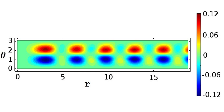
(e)  

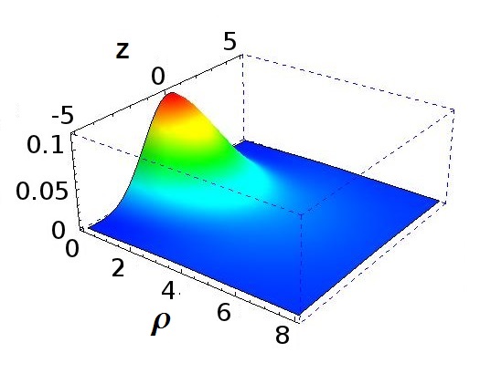
(f)  

Figure 1: Solution profile functions in the leading order: (a) ${\tilde{K}}_{1}$; (b) ${\tilde{K}}_{2}$; (c) ${\tilde{K}}_{4}$; (d) ${\tilde{K}}_{5}$; (e) the time averaged radial color magnetic field $\bar{B}_{r}^{3}$; (f) the time averaged energy density $\bar{\cal E}(\rho,z)$ in the plane $(\rho,z)$ in cylindrical coordinates ($g=1,M=1$).

and it has non-vanishing time averaged radial color magnetic fields $\bar{B}^{3}_{r}=\langle F_{\theta\varphi}^{3}\rangle_{t}=-3/4{\tilde{K}}_{2}{\tilde{K}}_{4}$ and $\bar{B}^{8}_{r}=-\bar{B}^{3}_{r}$, Fig. 1e, which correspond to magnetic field distribution of a non-topological monopole-antimonopole pair plb2018 . The energy density of the solution is finite everywhere and decreases along the radial direction as $1/r^{2}$, Fig. 1f.

The obtained solutions possess a nice feature, they are invariant under the Weyl permutation group acting on $I,U,V$ sectors of $SU(2)$ subgroups. The classical Lagrangian on the space of field configurations satisfying the ansatz (2,3) has an explicit Weyl symmetric form

$${\cal L}_{Weyl}=\sum_{p=1,2,3}\Big{\{}-\dfrac{1}{6}(F_{\mu\nu}^{p})^{2}-\dfrac{1}{2}|\partial_{\mu}W_{\nu}^{p}-\partial_{\nu}W_{\mu}^{p}|^{2}-$$

$$\dfrac{9}{4}\Big{[}(W^{*p\mu}W^{p}_{\mu})^{2}-(W^{*p\mu}W^{*p}_{\mu})(W^{p\nu}W^{p}_{\nu})\Big{]}\Big{\}},$$ (5)

where index “p” corresponds to $I,U,V$ subgroups $SU(2)$, and we use complex notations for the gauge potentials SM2 ; flyvb ; mpla2006 . Note that ansatz (2, 3) fixes the local gauge symmetry, however, the Lagrangian ${\cal L}_{Weyl}$ and corresponding solutions are still invariant under the action of the finite Weyl color group. While the local gauge symmetry determines dynamical laws by means of equations of motion, the global Weyl symmetry defines the symmetry of physical states and observables. In a particular, the Weyl symmetry implies an important identity, $A_{\varphi}^{3}\equiv A_{\varphi}^{8}$, which determines an absolute minimum of the effective potential flyvb ; mpla2006 , i.e., the vacuum energy.

It is remarkable, the Weyl symmetric solutions reveal the phenomenon of Abelian projection. To show this, one observes that a regular single valued solution, Fig. 1, is uniquely defined (up to conformal scaling transformation) by an amplitude of the Abelian field $K_{4}$ and by a choice of $\theta$-angle modes of the Fourier components ${\tilde{K}}_{i}(r,\theta)$, (4). The Abelian projection of the solution corresponds to the limit of vanishing off-diagonal gauge fields $K_{1,2,5}$ with a remaining Abelian potential $K_{4}$ which satisfies the Maxwell type equation.

It is surprising, that the non-Abelian solutions presented in Fig. 1 and in plb2018 admit an Abelian dominance effect. A careful numeric analysis shows that a contribution of the lowest $\theta$-angle mode ${\tilde{K}}_{4}(Mr,\theta)$ to the total energy is $95\%\pm 1.5\%$ SM2 . The obtained value is very close to the known estimate of Abelian dominance established before only for the Wilson loop functional abeldom1 ; abeldom3 . Note that an Abelian gauge potential is not itself gauge invariant. However, the Abelian projection, applied to physical gauge invariant quantities like a a quantum effective action, produces gauge invariant results. It has been proved, that a quantum effective action with an Abelian external background field is invariant under local gauge transformations reinhardt97 . We conclude, that the QCD vacuum structure is determined by regular Weyl symmetric Abelian solutions which represent fixed points in the configuration space under the Weyl group transformation. This is a direct evidence of the Abelian projection conjectured by ‘t Hooft thooft81 . The existence of Weyl symmetric Abelian solutions might not be surprising, since the Weyl group leaves the Abelian subgroup invariant by definition. A surprising result is that there are non-Abelian solutions which represent fixed points under the Weyl group transformation in the whole configuration space of $SU(3)$ Lie algebra valued gauge fields.

So far we have considered a case of axially-symmetric fileds. In a general case, the Weyl symmetric Abelian projected QCD is equivalent to an Abelian gauge theory with a gauge potential $A_{\mu}=A_{\mu}^{3,8}$ corresponding to a compact structure group $U(1)$. A complete set of spherical wave solutions to the Maxwell equations is given by the vector spherical harmonics (in a temporal gauge $A_{t}=0$) jackson ; eisenberg

$$\vec{A}_{lm}^{\mathfrak{m}}=\dfrac{1}{\sqrt{l(l+1)}}\vec{L}j_{l}(kr)Y_{lm}(\theta,\varphi)e^{i\omega t},$$

$$\vec{A}_{lm}^{\mathfrak{e}}=\dfrac{-i}{\sqrt{l(l+1)}}\vec{\nabla}\times(\vec{L}j_{l}(kr)Y_{lm}(\theta,\varphi))e^{i\omega t},$$

$$\vec{A}_{lm}^{\mathfrak{l}}=\dfrac{1}{k}\vec{\nabla}j_{l}(kr)Y_{lm}(\theta,\varphi)e^{i\omega t},$$ (6)

where $\omega=kc$, $\{\vec{A}_{lm}^{\mathfrak{m,e,l}}\}$ are eigenfunctions of the total angular momentum operator with $J=l\geq 1$, $J_{z}=m$, and the superscripts $\mathfrak{m,e,l}$ denote magnetic, electric and longitudinal modes respectively. We neglect the longitudinal mode as unphysical and keep only transverse modes satisfying the constraints $\operatorname{Div}\vec{A}=0$ and $\vec{E}\cdot\vec{B}\equiv 0$. One has still the Abelian dominance effect since the energy spectrum of general stationary solutions is degenerated with respect to the quantum number ${}^{\prime\prime}m^{\prime\prime}$ due to invariance under the group $SO(3)$ of space rotations.

The most important step in establishing the vacuum structure is to prove the quantum stability of Abelian solutions (6) at microscopic level, i.e., in any small vicinity of each space-time point. We prove this by solving a “Schrödinger” eigenvalue equation for quantum gluon fluctuation modes $\Psi_{\mu}^{a}$ plb2018

$$\mathscr{K}_{\mu\nu}^{ab}\Psi_{\nu}^{b}=\lambda\Psi_{\mu}^{a},$$

$$\mathscr{K}_{\mu\nu}^{ab}=-\delta^{ab}\delta_{\mu\nu}\partial^{2}_{t}-\delta_{\mu\nu}({\mathscr{D}}_{\rho}{\mathscr{D}}^{\rho})^{ab}-2f^{acb}{\mathscr{F}}_{\mu\nu}^{c},\quad$$ (7)

where the operator $\mathscr{K}_{\mu\nu}^{ab}$ corresponds to one-loop gluon contribution to the effective action plb2018 , and $\mathscr{D}_{\mu},\mathscr{F}_{\mu\nu}$ are defined by means of background Abelian solution (6). The existence of a negative eigenvalue $\lambda$ would indicate to the presence of an unstable mode which destabilizes the vacuum. We solve numerically the eigenvalue equation (Microscopic vacuum structure in a pure QCD) with an axially-symmetric background Abelian field, $m=0$, for various values of the parameters $(l,M)$ and radial size $L$ of the numeric space domain. Our numeric analysis confirms the positiveness of the spectrum of the operator $K_{\mu\nu}^{ab}$ for parameter values $l\leq 4$ and $\nu_{11}\leq M\leq 10$, $\nu_{11}\leq L\leq 200$. Typical time dependent fluctuation modes corresponding to the lowest eigenvalue are shown in Fig. 2 (details of calculation are enclosed in SM2 ). It is somewhat unexpected, that standing wave solutions of electric type are stable as well SM2 , contrary to a case of constant chromoelectric field schan . This proves that transverse Abelian solutions (6) can serve as structural elements of a stable vacuum.

(a)  

(b)  

Figure 2: Gluon fluctuation modes with the lowest eigenvalue $\lambda=0.0292$ for the vacuum magnetic field with ($l=1,m=0)$: (a) $\Psi_{3}^{2}$; (b) $\Psi_{4}^{1}$ ($g=1,M=1$).

We quantize the Abelian solutions (6) in a finite space region constrained by a sphere of radius $a_{0}$ corresponding to an effective glueball size. It is suitable to introduce dimensionless units $\tilde{M}=Ma_{0},x=r/a_{0},\tau=t/a_{0}$. To find proper boundary conditions we require that the Pointing vector $\vec{\mathbf{S}}=\vec{\mathbf{E}}\times\vec{\mathbf{B}}$ vanishes on the sphere. This implies two possible types of boundary conditions

$$(I): \vec{A}_{lm}^{\mathfrak{m,e}}(\tilde{M}x)|_{x=1}=0,~{}\tilde{M}_{nl}=\mu_{nl},$$

$$(II): \partial_{r}(r\vec{A}_{lm}^{\mathfrak{m,e}}(\tilde{M}x))|_{x=1}=0,~{}\tilde{M}_{nl}=\nu_{nl},$$ (8)

where $\mu_{nl}$ are nodes of the Bessel function $j_{l}(r)$, and $\nu_{nl}$ denote zeros of the function $\partial_{r}(rj_{l}(r))$, the integers $(n\geq 1,l\geq 1)$ are the main and orbital quantum numbers. Our approach resembles the old MIT bag models MIT1 ; MIT2 ; MIT3 where the energy spectrum of free glueballs was obtained for the first time jaffe1976 ; johnson1981 ; jaffe1986 . However, there are principal differences between our formalism and bag models: (i) we apply the Weyl symmetric Abelian projection which leads directly to physical quantum states; (ii) in bag models one has to impose an additional constraint $n_{\mu}F^{\mu\nu}=0$, ($n_{\mu}=(0,\vec{n}\equiv\vec{r}/r)$) MIT3 which prevents the color charge to pass through the bag surface.

We choose the following normalization condition for the vector harmonics $\vec{A}_{{\tilde{M}}lm}^{\mathfrak{m,e}}$

$$\dfrac{1}{4\pi}\int_{0}^{1}dx\int d\theta d\varphi x^{2}\sin\theta(\{\vec{A}_{{\tilde{M}}_{nl}lm}^{\mathfrak{m,e}})^{2}=\dfrac{1}{{\tilde{M}}_{nl}}.$$ (9)

The standard canonical quantization results in the following Hamiltonian expressed in terms of the creation and annihilation operators $c^{\pm}_{nl}$

$$H=\dfrac{1}{2}\sum_{n,l,m}\tilde{M}_{nl}(c^{+}_{nlm}c^{-}_{nlm}+c^{-}_{nlm}c^{+}_{nlm}).$$ (10)

One particle states $\{c^{+}_{nlm}|0\rangle\}$ describe primary free Abelian glueballs. The knowledge of explicit solutions for the vector potential (6) allows to estimate densities of various vacuum gluon condensates. Averaged over the time and polar angle vacuum gluon condensates $\alpha_{s}\langle(F_{\mu\nu})^{2}\rangle$ corresponding to magnetic modes $\vec{A}_{\nu_{11}11}^{\mathfrak{m}}$ and $\vec{A}_{\mu_{11}11}^{\mathfrak{m}}$ are depicted in Fig. 3 ($\alpha_{s}=0.5$ PDG ).

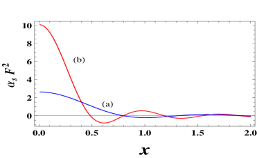
Figure 3: Radial densities of the magnetic vacuum gluon condensates $\alpha_{s}\langle\overline{F^{2}}\rangle$ corresponding to modes $\nu_{11}=2.74...$, (a), and $\mu_{11}=4.49...$, (b); (n=l=1, m=0).

The oscillating behavior of the vacuum gluon condensate density was obtained before within the instanton approach to QCD dorokhov1997 ; dorokhov2000 . Integrating the gluon condensate density over the interval $(0\leq x\leq 1)$ one can fit the value of the vacuum gluon condensate, $\alpha_{s}\langle(F_{\mu\nu}^{a})^{2}\rangle=(540MeV)^{4}$, by fixing the effective glueball size parameter, $a_{0}=0.376Fm$. With this, the energy spectrum of free Abelian glueballs $J^{PC}$ is $E_{nl}=197\tilde{M}_{nl}/a_{0}$ MeV ($J=l$, $P=(-1)^{J+1}$ for magnetic glueballs and $P=(-1)^{J}$ for electric glueballs, $C=-1$ jackson ; eisenberg ). Two lightest glueballs, $(1)^{+-},(1)^{--}$ of magnetic and electric types respectively, have the same energy $E_{11}=1.435$ GeV corresponding to antinode $\nu_{11}$.

Certainly, the primary free glueballs are not observable quantities since we have not taken into account their interaction to vacuum gluon condensate. To estimate the effect of such interaction we use a method applied in study of the anomalous magnetic moment of a photon propagating in the external magnetic field magnphoton1 ; magnphoton2 . In QCD the role of an external magnetic field is played by the magnetic vacuum gluon condensate. Consider one-loop $SU(3)$ effective Lagrangian ${\cal L}^{1-l}$ in constant field approximation savv ; flyvb

$${\cal L}^{1-l}=-\dfrac{1}{4}{\tilde{F}}^{2}-k_{0}g^{2}{\tilde{F}}^{2}\Big{(}\log(\dfrac{g^{2}{\tilde{F}}^{2}}{\Lambda_{QCD}^{4}})-c_{0}\Big{)},$$ (11)

where ${\tilde{F}}_{\mu\nu}$ is an external Weyl symmetric Abelian color magnetic field, the factor $k_{0}=\dfrac{11}{64\pi^{2}}$ is proportional to 1-loop beta function, and $c_{0}$ is a renormalization constant. A corresponding one-loop effective potential implies a value $\simeq(70MeV)^{4}$ for the vacuum gluon condensate, which is not reliable. However, the most important property of the effective Lagrangian is the presence of essentially non-perturbative structure which leads to appearance of a non-trivial minimum of the effective potential. Such a structure allows to derive an effective Lagrangian for physical glueballs with setting $k_{0},c_{0}$ as free phenomenological parameters. Following the method in magnphoton1 ; magnphoton2 we split the external field ${\tilde{F}}_{\mu\nu}$ into two parts

$${\tilde{F}}_{\mu\nu}=B_{\mu\nu}+F_{\mu\nu},$$ (12)

where $B_{\mu\nu}=\partial_{\mu}B_{\nu}-\partial_{\nu}B_{\mu}$ describes the magnetic vacuum gluon condensate, and $F_{\mu\nu}=\partial_{\mu}A_{\nu}-\partial_{\nu}A_{\mu}$ contains the Weyl symmetric Abelian gauge potential $A_{\mu}$ describing the physical glueball. In approximation of slowly varied vacuum condensate we decompose the Lagrangian ${\cal L}^{1-l}$ around the vacuum field $B_{\mu\nu}$ corresponding to a non-trivial minimum of the effective potential at the value of vacuum gluon condensate

$$g^{2}B^{2}=\Lambda_{QCD}\exp\big{(}c_{0}-1-\dfrac{1}{2k_{0}g^{2}}\big{)}.$$ (13)

With this one obtains an effective Lagrangian for physical Abelian glueballs in quadratic approximation

$${\cal L}_{eff}^{(2)}[A]=-2k_{0}g^{2}\dfrac{(B^{\mu\nu}F_{\mu\nu})^{2}}{B^{2}}\equiv-\kappa(B^{\mu\nu}F_{\mu\nu})^{2},$$ (14)

where we neglect a term corresponding to an absolute value of the vacuum energy, and $\kappa$ is an effective coupling constant. The effective Lagrangian ${\cal L}_{eff}^{(2)}[A]$ is strikingly different from a corresponding effective Lagrangian in QED magnphoton1 ; magnphoton2 . Namely, the expression (14) does not include the classical kinetic term $-1/4F_{\mu\nu}^{2}$ which has disappeared due to non-perturbative origin of the vacuum gluon condensate (13). Note that result (14) is model independent, and it can be obtained from a class of Lagrangian functions which admit series expansion around a non-trivial vacuum.

In a case of the lightest magnetic glueball the vacuum gluon condensate is described by the vector harmonic $\vec{A}_{l=1,m=0}^{\mathfrak{m}}$, $\omega=\nu_{11}$, with one non-zero component

$$B_{\varphi}(x,\theta,\tau)=N_{11}xj_{1}(\nu_{11}x)\sin^{2}\theta\sin(\nu_{11}\tau),$$ (15)

where $N_{11}$ is a renormalization constant. The lightest magnetic glueball is described by the gauge potential $A_{\varphi}(x,\theta,\tau)$ which assumed to be time-coherent to the vacuum condensate field, $A_{\varphi}(x,\theta,\tau)=a(x,\theta)\sin(\nu_{11}\tau+\phi_{0})$, with a constant phase shift $\phi_{0}$. A time-averaged effective Lagrangian ${\cal L}_{eff}^{(2)}[A]$ leads to Euler equation for the field $a(x,\theta)$ SM2 . The equation is separable and implies an ordinary differential equation for a spherically symmetric function $a(x,\theta)\equiv f(x)$

$$r^{2}b^{\prime 2}f^{\prime\prime}-2b^{\prime}(b+xb^{\prime}-x^{2}b^{\prime\prime})f^{\prime}-$$

$$\nu_{11}^{2}\Big{(}\nu_{11}^{2}x^{2}b^{2}-\xi\nu_{11}^{2}x^{3}j_{2}(\nu_{11}x)b^{\prime}2\Big{)}f=0,$$ (16)

where $b(x)=\nu_{11}xj_{1}(\nu_{11}x)$, $\xi\equiv\cos(2\phi_{0})/(2+\cos(2\phi_{0}))$. The coefficient functions in front of the first and second derivative terms in (16) vanish at $x_{0}=1$ (or $r_{0}=a_{0})$. This implies that a regular solution is localized inside a finite interval $0\leq x\leq 1$, Fig. 4a.

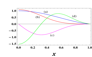
Figure 4: (a) Solution $f(x)$ with a unit initial amplitude; (b) a corresponding radial energy density $\bar{\cal E}/4\pi\kappa$; (c) the first derivative of the energy density; (d) the second derivative of the energy density; $\phi_{0}=\pm\pi/2$.

The solution has a removable singularity at $x_{0}=1$. To verify that solution is physical we check the properties of the energy density averaged over the time and polar angle

$$\bar{\cal E} = \dfrac{\pi\kappa}{4x^{2}}\Big{(}(2+\cos(2\phi_{0}))b^{2}f^{2}+2\cos(2\phi_{0})bb^{\prime}ff^{\prime}$$ (17)

$$+(2+\cos(2\phi_{0}))b^{\prime 2}f^{\prime 2}\Big{)}.$$

One can verify that the energy density and its first and second derivatives are continious functions at $x_{0}=1$, Fig. 4bcd. The solution with the phase shift value $\phi_{0}=\pm\pi/2$ has a minimal energy, and the corresponding effective Lagrangian vanishes identically as for the photon plane wave. So the obtained solution for the physical glueball is stable, it does not collapse and has the energy upper bound $1.435$ GeV provided by the energy of the lightest free glueball.

In QED the photon anomalous magnetic moment leads to changing the total angular momentum magnphoton2 . A similar effect in QCD provides the total angular momentum $J=0$ for the physical glueball. Quantum numbers of the glueball interacting to vacuum magnetic gluon condensate are defined in the same way as for two photon system landau2photon ; yang2photon ; minkowski2photon and lead to two lightest magnetic glueballs $0^{++},0^{-+}$ which might be identified with the expected lightest two-gluon glueballs kochelev2009 ; ochs2013 . Note that the lightest free electric glueball $1^{+-}$ does not interact to vacuum magnetic condensate due to the structure of the effective Lagrangian ${\cal L}_{eff}^{(2)}[A]$. So that it is fictious in agreement with the Yang theorem ochs2013 ; yang2photon .

In conclusion, the proposed microscopic description of a pure QCD vacuum reveals the Weyl symmetric Abelian projection and Abelian dominance phenomenon. This allows to describe a full pure glueball spectrum endowed with a fine structure generated by off-diagonal gluons. A detailed structure of the pure glueball spectrum and generalization to QCD with quarks will be considered in a separate paper.

- (1) Y. Nambu, Phys. Rev. D10, 4262 (1974).
- (2) S. Mandelstam, Phys. Rep. 23C, 245 (1976).
- (3) A. Polyakov, Nucl. Phys. B120, 429 (1977).
- (4) G. ’t Hooft, Nucl. Phys. B190, 455 (1981).
- (5) H.B. Nielsen and P. Olesen, Nucl. Phys. B160, 380 (1979).
- (6) J. Ambjørn and P. Olesen, Nucl. Phys. B170, 265 (1980).
- (7) M. Chernodub, Phys. Lett. B730, 63 (2014).
- (8) M. Engelhardt, K. Langfeld, H. Fardt, O. Tennert, Phys. Rev. D61, 054504 (2000).
- (9) J. Greensite, EPJ Web Conf., Vol. 137, 01009 (2017).
- (10) P. Olesen, A center vortex representaton of the classical SU(2) vacuum, arXiv: 1605.00603 (2016).
- (11) D. Diakonov, V. Petrov, AIP Conf. Proc. 1343 (2011) 69-74.
- (12) G.K. Savvidy, Phys. Lett. B71, 133 (1977).
- (13) N.K. Nielsen and P. Olesen, Nucl. Phys. B144, 376 (1978).
- (14) H. Weyl, Symmetry, Princeton Univ. Press, 1952, p. 144.
- (15) R. Dashen, B. Hasslacher and A. Neveu, Phys. Rev. D10 (1974) 4138.
- (16) D.G. Pak, B.-H.- Lee, Y. Kim, T. Tsukioka, P.M. Zhang, Phys. Lett. B 780, (2018) 479.
- (17) Y. Ne’eman, Symm.: Culture and Science, 10, 143 (1999).
- (18) D.G. Pak, P.M. Zhang, Microscopic vacuum structure in a pure QCD – Supplemental Material.
- (19) H. Flyvbjerg, Nucl. Phys. B176, 379 (1980).
- (20) Y.M. Cho, J.H. Kim, D.G. Pak, Mod. Phys. Lett. A21, 2789 (2006).
- (21) A. Kronfeld, G. Schierholz and U. Wiese, Nucl. Phys. B 293, 461 (1987).
- (22) T. Suzuki and I. Yotsuyanagi, Phys. Rev. D 42, 4257 (1990).
- (23) H. Reinhardt, Nucl. Phys. B 503 (1997) 505.
- (24) J. D. Jackson, Classical Electrodynamics, Wiley, New Jersey, 1999.
- (25) J.M. Eisenberg, W. Greiner, Nuclear Theory 2: Excitation Mechanisms Of The Nucleus, North Holland, 1970.
- (26) V. Schanbacher, Phys. Rev. D 26, (1982) 489.
- (27) A. Chodos, R.L. Jaffe, K. Johnson, C.B. Thorn, and V.F. Weisskopf, Phys. Rev. D9, 3471 (1974).
- (28) T. DeGrand, R.L. Jaffe, K. Johnson, and J. Kiskis, Phys. Rev. D12, 2060 (1975).
- (29) K. Johnson, Acta Phys. Pol. 6 (1975) 865.
- (30) R.L. Jaffe and K. Johnson, Phys. Lett. 60B, 201 (1976).
- (31) J.F. Donoghue, K. Johnson and B. A. Li, Phys. Lett. 99B, 416 (1981).
- (32) R.L. Jaffe and K. Johnson and Z. Ryzak, Ann. of Phys. 168, 344 (1986).
- (33) M. Tanabashi et al. (Particle Data Group), Phys. Rev. D 98, 030001 (2018).
- (34) A.E. Dorokhov, S.V. Esaibegian, S.V. Mikhailov, Phys. Rev. D56 (1997) 4062.
- (35) A.E. Dorokhov, S.V. Esaibegian, A.E. Maximov, S.V. Mikhailov, Eur. Phys. J. C13 (2000) 331.
- (36) H.P. Rojas and E.R. Querts, Phys. Rev. D79, 093002 (2009).
- (37) S. Villalb-Chavez and A.E. Shabad, Phys. Rev. D86, 105040 (2012).
- (38) L.D. Landau, Dokl. Akad. Nauk SSSR 60, 207 (1948).
- (39) C.N. Yang, Phys. Rev. 77, 242 (1950).
- (40) P. Minkowski, Fizika B 14, 79 (2005).
- (41) V. Mathieu, N. Kochelev, V. Vento, Int. J. Mod. Phys. E18 (2009) 1.
- (42) W. Ochs, J. Phys. G: Nucl. Part. Phys. 40 (2013) 043001.