A model for calorimetric measurements in an open quantum system

Abstract

We investigate the experimental setup proposed in [New J. Phys., 15, 115006 (2013)] for calorimetric measurements of thermodynamic indicators in an open quantum system. As theoretical model we consider a periodically driven qubit coupled with a large yet finite electron reservoir, the calorimeter. The calorimeter is initially at equilibrium with an infinite phonon bath. As time elapses, the temperature of the calorimeter varies in consequence of energy exchanges with the qubit and the phonon bath. We show how under weak coupling assumptions, the evolution of the qubit-calorimeter system can be described by a generalized quantum jump process including as dynamical variable the temperature of the calorimeter. We study the jump process by numeric and analytic methods. Asymptotically with the duration of the drive, the qubit-calorimeter attains a steady state. In this same limit, we use multiscale perturbation theory to derive a Fokker-Planck equation governing the calorimeter temperature distribution. We inquire the properties of the temperature probability distribution close and at the steady state. In particular, we predict the behavior of measurable statistical indicators versus the qubit-calorimeter coupling constant.

I Introduction

The measurement of thermodynamic quantities in an open quantum system poses considerable experimental challenges. The main reason is that one needs to find a way to monitor all the active degrees of freedom in the system and its environment.

The proposal of Pekola et al. (2013) is to detect quanta of energy absorbed or emitted by a driven quantum system by measuring the temperature variation of the environment surrounding it. More precisely, Pekola et al. (2013) considers an integrated quantum circuit including a superconducting qubit and a resistor element. A superconducting qubit is a two level artificial atom constructed from collective electrodynamic modes of a macroscopic superconducting element Büttiker (1987); Bouchiat et al. (1998). Superconducting qubits can be coupled with other linear circuit elements like capacitors, inductors, and transmission lines. This fact renders in principle possible to monitor energy exchanges of the qubit by constantly monitoring the temperature of a resistor element in the circuit. Hence, the realization of the experiment Pekola et al. (2013) essentially hinges upon the feasibility of measuring the temperature of the calorimeter sufficiently accurate over time scales shorter than the thermal relaxation time of the qubit. Recent developments of nano-scale radio-frequency thermometry permit to envisage the accomplishment of this goal. Already a decade ago, Schmidt et al. (2003) demonstrated the feasibility of measuring the temperature of the normal metal side of an SIN (Superconductor-Insulator-Normal metal) tunnel junction thermometer with a bandwidths of up to $100\,\mathrm{MHz}$. More recently, Gasparinetti et al. (2015); Viisanen et al. (2015) showed that SIN thermometry can operate down to temperatures of $100\,\mathrm{mK}$ and detect a $10\,\mathrm{mK}$ temperature spike in a single-shot measurement. This is not yet sufficient for calorimetric measurements of single microwave photons in superconducting quantum circuit, but makes the prospect of realizing the experiment Pekola et al. (2013) in the near future very concrete.

The aim of the present contribution is to theoretically explore features of the temperature process in Pekola et al. (2013). We take as starting point the theoretical qubit-calorimeter model introduced in Kupiainen et al. (2016). Accordingly, we describe the dynamics of the qubit-calorimeter system by a generalized quantum jump process Dalibard et al. (1992); Carmichael (1993). The generalization consists in treating as dynamical variable the temperature of the calorimeter together with the components of the state vector of the qubit. The derivation of the quantum jump process then follows from the usual set of assumptions presiding over the validity of the Markovian approximation (see for example Breuer and Petruccione (2002)) and the hypothesis that in between interactions with the qubit the calorimeter behaves as a Fermi gas in local equilibrium. In other words, the calorimeter is modelled by a collection of grand-canonical ensembles parametrized by a temperature evolving in time according to a prescribed dynamics. Extended statistical ensembles characterized by a dynamically determined temperature come naturally about, for example in the study of energy exchanges between a single electron box tunnel coupled to metallic reservoir van den Berg et al. (2015), and in macroscopic statistical physics for example as a tool to optimize Monte Carlo methods Marinari and Parisi (1992).

As a step towards increased realism, we advance the model of Kupiainen et al. (2016) in two ways. First, we suppose that the qubit is strongly coupled with a periodic control field. Drawing on Breuer and Petruccione (1997), we obtain the corresponding stochastic Schrödinger equation for the qubit. Second, we include in the model normal metal electron-phonon interactions between the calorimeter and the environment. Electron-phonon interactions bring about a drift and a noise term in the stochastic differential equations governing the calorimeter temperature Kaganov et al. (1957); Wellstood et al. (1994); Pekola and Karimi (2018).

We then inquire the behaviour of the probability distribution of temperature $T_{e}$ of the calorimeter by numeric and analytic methods and for experimentally relevant values of the parameters. We show that as the duration of the drive increases the temperature distribution tends to an equilibrium state. In order to shed more light on the asymptotic stage of the dynamics, we take advantage of the time-scale separation between the characteristic relaxation times of the qubit and the temperature process and show by means of multiscale perturbation theory Pavliotis and Stuart (2008) that the temperature probability distribution evolves asymptotically according to a Fokker-Planck equation Gardiner (2009). The Fokker–Planck equation evinces the general form of dependence upon the phonon temperature $T_{p}$ and the qubit-calorimeter coupling $g$ of the steady state temperature $T_{S}$ and the temperature distribution relaxation time to equilibrium $\tau_{S}$.

The structure of the paper is as follows. In section II we briefly sketch the experimental setup of Pekola et al. (2013). In section III we introduce the qubit-calorimeter model whose dynamics in the Markovian limit we subsequently present in section IV. In section V we inquire the asymptotic behavior of the temperature probability distribution by multiscale methods. Finally, we report on our numeric investigation of the model in section VI. We focus on two regimes. The first regime or ”short time regime” is 10 periods of resonant frequency. In this time the qubit and temperature only make a few jumps. The second regime or the ”long time” regime is of the order of $10^{4}$ periods of resonant frequency. On this time scale the system makes many jumps and drift term due to the phonons becomes important. In the physically relevant parametric range, the results of the simulations are in good agreement with the analytic predictions of section V.

Finally, we defer most of the technical calculations to the appendices.

II The Qubit-Calorimeter circuit

Superconducting qubits are solid state devices behaving according to the rules of quantum mechanics. They combine the feature, characteristic of atoms, of exhibiting quantized energy levels with the flexibility of linear circuit elements which can be connected in more complex networks. The realization of a superconducting qubit plays upon the properties of Josephson tunnel junctions Büttiker (1987); Leggett (1992). Namely, at temperatures sufficiently low to render thermal noise negligible, Josephson tunnel junctions maintain quantum coherence of charge transport (i.e. are non-dissipative) governed by a non-harmonic Hamiltonian (see e.g. Bouchiat et al. (1998); Devoret et al. (2003); Devoret and Schoelkopf (2013)). Non-linear separation of the energy levels, is essential to prevent qubit operations from exciting transitions between more than two states in the system.

In Figure (1(a)) we draw a quantum integrated circuit of the type envisaged in Pekola et al. (2013). The circuit contains a transmon qubit Koch et al. (2007). A transmon qubit consists of a superconducting island coupled through Josephson junctions and shunted by a capacitor. The transmon qubit is embedded in a resonance circuit to amplify its signal. The resistor element in the circuit (bright blue online in figure (1(a))) is the calorimeter, making it into an open quantum system. In the current work we do not consider the resonator, but model the qubit to be directly coupled to the calorimeter. We conceptualize the calorimeter as a gas of free electrons weakly interacting with an infinite phonon thermal bath. Phonons describe excitations of the lattice structure of the normal metal in the resistor and in the circuit substrate. The phonon bath is maintained at a uniform constant temperature $T_{p}$ equal to that of the cryostat. The temperature $T_{e}$ of the electron gas is in equilibrium with the phonon bath at the beginning of the experiment. The drive is an external periodic control potential initially turned-off. When turned on, the drive excites transitions in the qubit. The temperature of the resistor varies then in consequence of the single microwave photons emitted or absorbed by the two-level system. The actual temperature measurement happens via a Normal metal-Insulator-Superconductor (N I S) junction Schmidt et al. (2003); Gasparinetti et al. (2015); Viisanen et al. (2015) on the resistor. This is possible because the conductance $G$ of the N I S junction depends on the temperature $T_{e}$ of the normal metal whereas it is independent of the temperature of the superconductor:

$$G=\int_{\mathbb{R}}\frac{\mathop{}\!\mathrm{d}E\,N_{S}(E)}{R_{T}\,k_{\mathrm{B}}\,T_{e}}f_{T_{e}}(E-e\,V_{b})\big{[}1-f_{T_{e}}(E-e\,V_{b})\big{]}.$$

Here, $N_{S}(E)$ is the normalized Bardeen-Cooper-Schrieffer superconducting density of states, $k_{\mathrm{B}}$ is Boltzmann constant and $f_{T_{e}}(E)=(1+\exp(E/k_{\mathrm{B}}T_{e}))^{-1}$ the Fermi–Dirac distribution at temperature $T_{e}$ with $E$ referenced to the chemical potential Giazotto et al. (2006). $V_{b}$ and $R_{T}$ are respectively the voltage bias and the resistance of the N I S junction.

(a) The quantum integrated circuit of Pekola et al. (2013). The temperature measurement is performed by embedding an N I S junction in a resonance circuit. The calorimeter consists of the electrons in the normal metal. The transmon qubit is formed by a Cooper pair box embedded in a resonance circuit. This figure is not up to scale. The Cooper pair box is of the order of 10 $\mu$m, the resonance circuit which it is embedded in is of the order of 1 mm, and the calorimeter is 1 $\mu$m.

(b) The qubit-calorimeter experiment as modelled by the Hamiltonian (1).

Figure 1: Visual representation of the quantum integrated circuit and its mathematical model.

III Theoretical Model

Figure 1(b) graphically illustrates our mathematical model of the qubit-calorimeter-phonon interactions. The Schrödinger picture Hamiltonian of the full quantum system is the sum

$$H=H_{q}+H_{qe}+H_{e}+H_{ep}+H_{p}$$ (1)

of the qubit $H_{q}$, the qubit-electron interaction $H_{qe}$, the electron gas $H_{e}$, the electron-phonon interaction $H_{ep}$ and the phonon $H_{p}$ Hamiltonians.

The Hamiltonian of the qubit is

$$H_{q}(t)=\frac{\hbar\,\omega_{q}}{2}\sigma_{z}+\kappa\,V_{d}(t)$$ (2)

where $\sigma_{z}$ denotes the diagonal Pauli matrix. The Hamiltonian is time non-autonomous owing to the presence of the driving potential $V_{d}(t)$. The drive is periodic with frequency $\omega_{L}$ and is strongly coupled with the qubit by the non-dimensional parameter $\kappa$. In consequence, it is expedient to resort to Floquet theory to describe the periodically driven qubit dynamics Shirley (1965); Zel’dovich (1967); Sambe (1973) see also Grifoni and Hänggi (1998); Holthaus (2015); Donvil (2018) and appendix A.

The qubit is directly coupled only to the calorimeter via the Hamiltonian

$$H_{qe}=g\,\frac{\sqrt{8\,\pi}\,\epsilon_{F}}{3\,N}\sum_{k\,\neq\,l\,\in\,\mathbb{S}}(\sigma_{+}+\sigma_{-})\,a^{\dagger}_{k}\,a_{l}$$ (3)

Here $\sigma_{+}$ and $\sigma_{-}$ are the qubit raising and lowering operators in the absence of external drive $V_{d}$. Similarly, $a_{k}$ and $a_{k}^{\dagger}$ are the annihilation and creation operators of a free fermion with energy specified by the absolute value $k$ of its wave number $\bm{k}$. The sum in (3) is restricted to an energy shell $\mathbb{S}$ close to the Fermi energy $\epsilon_{F}$ of the metal in the resistor. The sum ranges over non-diagonal terms to avoid trivial renormalization of the energy levels of the non-interacting Hamiltonians $H_{q}$ and $H_{e}$. We choose the numerical prefactor in (3) for computational convenience. The interaction is strength is characterised by the non-dimensional constant $g\,\ll\,1$, and $\epsilon_{F}$ sets the energy scale. Finally, $N=O(10^{9})$ is the number of electrons in the shell $\mathbb{S}$.

Of the remaining three terms on the right hand side of (1), $H_{e}$ and $H_{p}$ are the free fermion and boson gases Hamiltonians weakly coupled by a Frölich interaction term $H_{ep}$ Fröhlich (1952) (see for example chapter 9 of Mahan (2011)). As these Hamiltonians are textbook knowledge, we defer explicit expressions and quantitative analysis to appendix C. Here we discuss the qualitative picture. Phonons describe small vibrations in the lattice structure of the metal and its substrate. Phonon-self interactions can be neglected as the vibration amplitude is small with respect to the characteristic length of the lattice cell $O(k_{F}^{-1})$ for $k_{F}$ the Fermi wave vector Ashcroft and Mermin (1976). Electron self-interactions are re-absorbed in the parameters of the free energy spectrum. Namely, the typical relaxation rate to the Fermi–Dirac energy distribution of Landau quasi-particle in a metallic wire is of the order of $\tau_{ee}\sim 1$ ns Pothier et al. (1997), whereas electron-phonon interactions typically occur on a $\tau_{ep}\sim 10^{4}$ ns time-scale Gasparinetti et al. (2015). Thus, at any instant of time the state of phonons and electrons is described by quantum statistical equilibrium ensembles at well defined temperatures respectively denoted by $T_{p}$ and $T_{e}$. Within leading order accuracy, equilibrium states are perturbed by the deformation term $H_{ep}$. In the presence of small differences between $T_{p}$ and $T_{e}$, the perturbation results in a mean energy current $J\propto T_{p}^{5}-T_{e}^{5}$ Kaganov et al. (1957); Wellstood et al. (1994) with root mean square fluctuations $O(T_{p}^{3})$ Pekola and Karimi (2018). Experiments at sub-Kelvin temperatures clearly support these theoretical estimates.

IV Qubit-Calorimeter Process

Typical transmon qubit relaxation times are of the order of $\tau_{R}\sim 2-5\times 10^{5}$ ns Wang et al. (2015). The time scale separation $\tau_{ee}/\tau_{R}\sim 10^{-5}$, suggests describing the qubit dynamics in the Born–Markov approximation. The Markovian approximation is consistent with complete positivity of the state operator if we retain only secular terms in the evaluation of transition rates Breuer and Petruccione (2002). The rotating wave approximation offers a systematic procedure to neglect non-secular terms. It is justified if transitions among quasi-energy levels (see appendix A) in the qubit occur with rates much smaller than the corresponding frequency gaps in the radiation spectrum emitted by the qubit Breuer and Petruccione (1997, 2002). In other words, we need to work under the hypothesis that characteristic time scale $\tau_{qe}$ of the qubit-calorimeter interaction is much larger than the time $\tau_{m}$ set by the typical inverse separation of peaks in the radiation spectrum. In the weak-coupling limit, Fermi’s golden rule self-consistently yields the estimate $\tau_{eq}\sim g^{-2}$. We then expect the Markovian approximation to hold in the presence of a strongly coupled drive in (2) if $\tau_{m}\sim\kappa^{-1}$ holds so that $\tau_{m}/\tau_{eq}\sim g^{2}/\kappa\ll 1$. We verify this assumption in section VI for an explicit, experimentally relevant drive. Finally, the evaluation of qubit transition rates using the Fermi-Dirac distribution imposes $\tau_{eq}\,\ll\,\tau_{ep}\,\ll\,\tau_{R}$.

Under the above assumptions Kupiainen et al. (2016), we unravel the Markovian approximation for the qubit dynamics in the form of a Poisson-stochastic Schrödinger equation Breuer and Petruccione (1997, 2002)

$$\mathop{}\!\mathrm{d}\psi(t)=-\frac{\imath}{\hbar}\,G(\psi(t))\mathop{}\!\mathrm{d}t$$ (4)

$$+\sum_{|s|\leq 1}\sum_{|n|\leq\mathcal{N}}\left(\frac{A_{s,n}\psi(t)}{\|A_{s,n}\psi(t)\|}-\psi(t)\right)\mathop{}\!\mathrm{d}\nu_{s,n}(t)$$

The vector $\psi\in\mathbb{C}^{2}$ instantaneously specifies the state of the qubit. The sums on the right hand side ranges over the Lindblad operators

$$A_{s,n}=$$ (5)

$$\delta_{s,0}\,D_{1,1,n}\,\Big{(}|\phi_{1,0}(0)\rangle\langle\phi_{1,0}(0)|-|\phi_{0,0}(0)\rangle\langle\phi_{0,0}(0)|\Big{)}$$

$$+(\delta_{s,1}+\delta_{s,-1})\,D_{\frac{1+s}{2},\frac{1-s}{2},n}\,\Big{|}\phi_{\frac{1+s}{2},0}(0)\Big{\rangle}\Big{\langle}\phi_{\frac{1-s}{2},0}(0)\Big{|}.$$

By $\phi_{r,n}$ $r=0,1$, $n\in\mathbb{Z}$ we denote the element of the orthonormal basis in $\mathbb{C}^{2}\times\mathbb{L}^{2}[0,2\,\pi/\omega_{L}]$ associated to the quasi-energy level

$$\epsilon_{r,n}=\epsilon_{r}+n\,\hbar\,\omega_{L}$$ (6)

specified by Floquet theory (see appendix A and references therein). For any fixed $t$, the vector functions $\phi_{r,0}(t)$, $r=0,1$ form an orthonormal basis with respect to the standard scalar product in $\mathbb{C}^{2}$. The selection rules imposed by the matrix elements

$$D_{r,r^{\prime},n}=\frac{2\,\pi}{\omega_{L}}\int_{0}^{\frac{2\,\pi}{\omega_{L}}}\mathrm{d}t\,\langle\phi_{r,n}(t)|\sigma_{+}+\sigma_{-}|\phi_{r^{\prime},0}(t)\rangle$$ (7)

restrict the number of non-vanishing Lindblad operators (Breuer and Petruccione (1997, 2002) and appendix B). The representation (5) holds under the simplifying but not too restrictive assumption that there is a one to one correspondence between Lindblad operators and frequencies in the qubit radiation spectrum

$$\omega_{s,n}=s\,\frac{\epsilon_{0}-\epsilon_{1}}{\hbar}-n\,\omega_{L}$$ (8)

for $s=0,\pm 1$ and $n=0,\pm 1,\dots,\pm\mathcal{N}$. This assumption is reasonable if the selection rule (7) yields non-vanishing contribution only for a finite number of transitions, i.e. $\mathcal{N}<\infty$. In particular, it holds true for monochromatic drive we consider in section VI.

The evolution law (4) specifies a piecewise deterministic process. The deterministic evolution corresponds to a first order differential equation in $\mathbb{C}^{2}$ governed by the non-linear norm preserving drift

$$G(\psi)=$$ (9)

$$\frac{\imath\,\hbar}{2}\sum_{|s|\leq 1}\sum_{|n|\leq\mathcal{N}}\Gamma(\omega_{s,n},T_{e})(\|A_{s,n}\psi\|^{2}-A^{\dagger}_{s,n}A_{s,n})\psi$$

where $\|\cdot\|^{2}=\langle\cdot|\cdot\rangle$ is the squared norm in $\mathbb{C}^{2}$. The deterministic evolution is interrupted at random times by jumps modeled by the increment $\mathop{}\!\mathrm{d}\nu_{s,n}(t)$ of statistically independent Poisson processes for each $s,n$ and fully characterized by the conditional expectation

$$\mathbb{E}(\mathop{}\!\mathrm{d}\nu_{s,n}(t)|\psi)=\Gamma(\omega_{s,n},T_{e})\|A_{s,n}\psi\|^{2}\mathop{}\!\mathrm{d}t.$$ (10)

Here and in (9) the radiation frequency dependence of

$$\Gamma(\omega,T_{e})=\frac{g^{2}\,\omega\,e^{\hbar\omega/(k_{\mathrm{B}}T_{e})}}{e^{\hbar\omega/(k_{B}\,T_{e})}-1}.$$ (11)

stems from the fact that a leading order transitions in the qubit always involves creating and annihilating an electron in the calorimeter (see appendix B for details). For $\omega>0$ the calorimeter absorbs energy, for $\omega<0$ the calorimeter loses energy. The rates depend on the temperature of the electron bath $T_{e}$.

We determine the temperature $T_{e}$ from internal energy $E$ of the calorimeter using the Sommerfeld approximation, see e.g. Ashcroft and Mermin (1976). Under our working assumptions, $\mathrm{d}E$ is non-vanishing only over time-scales larger than $\tau_{eq}$. We obtain

$$\mathop{}\!\mathrm{d}T_{e}^{2}(t)=\frac{1}{N\,\gamma}\mathop{}\!\mathrm{d}E(t),$$ (12)

where

$$\gamma=\frac{\pi^{2}\,k_{B}^{2}}{4\,\epsilon_{F}}.$$ (13)

According to these definitions $N\,\gamma/2$ is the coefficient of the linear contribution to the heat capacity.

We identify two main contributions to the right hand side of (12):

$$\mathrm{d}E(t)=\mathrm{d}E_{eq}(t)+\mathrm{d}E_{ep}(t)$$

A jump in the qubit donates $\hbar\omega_{s,n}$ to the calorimeter. The corresponding instantaneous change in energy is

$$\mathrm{d}E_{eq}(t)=\sum_{|s|\leq 1}\sum_{|n|\leq\mathcal{N}}\hbar\omega_{s,n}\mathop{}\!\mathrm{d}\nu_{s,n}(t)$$ (14)

The increment $\mathrm{d}E_{ep}$ embodies the contribution of electron-phonon interactions. We model these interactions as the sum of a deterministic and a stochastic differential Kaganov et al. (1957); Wellstood et al. (1994); Pekola and Karimi (2018)

$$\mathrm{d}E_{ep}(t)=\Sigma V(T_{p}^{5}-T_{e}^{5}(t))\mathop{}\!\mathrm{d}t+\sqrt{10\Sigma Vk_{B}}T_{p}^{3}\mathop{}\!\mathrm{d}w(t).$$ (15)

Here $\mathrm{d}w(t)$ is the increment of a one-dimensional Wiener process, $\Sigma$ is a material constant defined in Appendix C, $V$ is the volume of the calorimeter and $T_{p}$ is the temperature of the phonon bath. The drift term in (15) tends to bring back the calorimeter into equilibrium with the phonon bath a temperature $T_{p}$. The Wiener increments models fluctuation of the heat current between the calorimeter and the phonon reservoir. Within leading accuracy, we evaluate the characteristic size of heat fluctuations by setting $T_{p}=T_{e}$. The diffusion coefficient in (15) does not prevent by construction realizations of the temperature process from acquiring nonphysical negative values. This means that (12) must be complemented by proper, e.g. reflecting, boundary conditions at $T_{e}=0$. Physically, the barrier at vanishing temperature can be understood observing that the energy distribution of a finite sized free-electron reservoir vanishes at low energies with a sharp drop to zero at the energy corresponding to the filled Fermi sea Pekola et al. (2016).

We are mainly interested in the evolution of the calorimeter temperature $T_{e}$. However, in order to obtain numerical results, it is necessary to simulate both processes: the evolution of the qubit (4) and the temperature (12) are coupled by (14), (15). Furthermore, the jump rates of the qubit (11) depend on the current temperature $T_{e}$ and on the current state of the qubit by equation (10). Quantitative predictions about evolution of the qubit-calorimeter system call for numeric investigation. It is, however, remarkable that in the long time limit, it is possible to derive a closed Fokker-Planck equation for the calorimeter temperature distribution, as we show in the next section.

V Effective Temperature Process

To start with, it is expedient to define the process $\xi(t)=T_{e}^{2}(t)$ which by (12) (14), (15) obeys the Wiener-Poisson stochastic differential equation

$$\mathrm{d}\xi(t)=\sum_{|s|\leq 1}\sum_{|n|\leq\mathcal{N}}\frac{\hbar\omega_{s,n}}{N\,\gamma}\mathop{}\!\mathrm{d}\nu_{s,n}(t)$$ (16)

$$+\frac{\Sigma V(T_{p}^{5}-\xi^{5/2}(t))\mathop{}\!\mathrm{d}t+\sqrt{10\Sigma Vk_{B}}T_{p}^{3}\mathop{}\!\mathrm{d}w(t)}{N\,\gamma}.$$

In Appendix D we show that the joint probability

$$P_{r}(X,t)=$$ (17)

$$\mathrm{P}\Big{(}X\leq\xi(t)<X+\mathrm{d}X\,\&\,\mbox{qubit in Floquet state}\,r\Big{)}$$

defined by (4), (16) obeys a closed time-autonomous Chapman–Kolmogorov master equation

$$\dot{P}_{r}(X,t)=\mathcal{L}_{X}P_{r}(X,t)$$ (18)

$$+\sum_{r^{\prime}=0,1}\int_{0}^{\infty}\mathrm{d}Y\,K_{rr^{\prime}}(X|Y)\,P_{r^{\prime}}(Y,t)$$

$$-\sum_{r^{\prime}=0,1}\int_{0}^{\infty}\mathrm{d}Y\,K_{r^{\prime}r}(Y|X)P_{r}(X,t).$$

The differential operation $\mathcal{L}_{X}$ represents the effect of electron-phonon interactions

$$\mathcal{L}_{X}P_{r}(X,t)= -\frac{\Sigma V}{N\,\gamma}\partial_{X}\big{(}(T_{p}^{5}-X^{5/2})P_{r}(X,t)\big{)}$$

$$+\frac{(\sqrt{10\Sigma Vk_{p}}T_{p}^{3})^{2}}{2\,N^{2}\,\gamma^{2}}\partial_{X}^{2}P_{r}(X,t).$$ (19)

The kernel $K$ describes quantum jumps

$$K_{rr^{\prime}}(X|Y)=$$ (20)

$$\sum_{n\leq|\mathcal{N}|}\mathcal{G}_{r,r^{\prime},n}(Y)\,\delta\left(Y-X+\frac{\hbar\,\omega_{r^{\prime}-r,n}}{N\,\gamma}\right)$$

where

$$\mathcal{G}_{r,r^{\prime},n}(X)=\Gamma(\omega_{r-r^{\prime},n},\sqrt{X})\,|D_{r,r^{\prime},n}|^{2}$$ (21)

Chapman–Kolmogorov master equations of the type (18) are compatible with the existence of an $H$-theorem, see e.g. § 3.7.3 of Gardiner (2009). We expect therefore that in the limit of long duration of the drive, (19) admits a steady state and that solutions corresponding to physical initial data relax to such steady state.

The occurrence of the non-dimensional weighting prefactor

$$\varepsilon=\frac{1}{N}$$

in (19) evinces the possibility to apply multiscale perturbation theory Pavliotis and Stuart (2008) to the asymptotic analysis of the master equation (18). Namely, we expect temperature equilibration to occur on a much longer time scale compared to the characteristic qubit relaxation time. Formally, if we posit

$$P_{r}(X,t)\equiv\tilde{P}_{r}(X,t,\varepsilon\,t)$$

we can couch the time derivative of the probability in terms of the sum of partial derivatives

$$\frac{\mathop{}\!\mathrm{d}P_{r}}{\mathop{}\!\mathrm{d}t}(X,t)=\partial_{t}\tilde{P}_{r}(X,t,\tau)+\varepsilon\,\partial_{\tau}\tilde{P}_{r}(X,t,\tau)$$ (22)

with respect to the “fast” variable $t$ and the “slow” one

$$\tau=\varepsilon\,t.$$

In the limit of long duration of the drive it is then reasonable to assume that the probability becomes stationary with respect to the fast time dependence

$$\partial_{t}\tilde{P}_{r}=0.$$

Therefore, under our working assumption

$$\bar{P}_{r}(X,\tau)\equiv\lim_{t\uparrow\infty}\tilde{P}_{r}(X,t,\tau)$$

satisfies

$$\varepsilon\,\partial_{\tau}\bar{P}_{r}(X,\tau)=\varepsilon\,\mathcal{L}_{X}^{(1)}\bar{P}_{r}(X,\tau)+\varepsilon^{2}\,\mathcal{L}_{X}^{(2)}\bar{P}_{r}(X,\tau)$$ (23)

$$+\sum_{s=0}^{1}\bigg{(}\mathds{G}^{(0)}_{r,s}(X)\bar{P}_{s}(X,\tau)-\mathds{G}^{(0)}_{s,r}(X)\bar{P}_{r}(X,\tau)\bigg{)}$$

$$+\sum_{k}^{\infty}\frac{\varepsilon^{k}}{k!}\sum_{s=0}^{1}\partial_{X}^{k}\bigg{(}\mathds{G}_{r,s}^{(k)}(X)\,\bar{P}_{s}(X,\tau)\bigg{)}$$

In (23) we use the notation

$$\mathcal{L}_{X}^{(1)}\bar{P}_{r}(X,\tau)=-\frac{\Sigma\,V}{\gamma}\partial_{X}\big{(}(T_{p}^{5}-X^{5/2})\bar{P}_{r}(X,\tau)\big{)}$$

$$\mathcal{L}_{X}^{(2)}\bar{P}_{r}(X,\tau)=\frac{(\sqrt{10\,\Sigma\,V\,k_{p}}T_{p}^{3})^{2}}{2\,\gamma^{2}}\partial_{X}^{2}\bar{P}_{r}(X,\tau)$$

and

$$\mathds{G}_{r,s}^{(k)}(X)=\sum_{|n|\leq\mathcal{N}}\left(\frac{\hbar\,\omega_{s-r,n}}{\gamma}\right)^{k}\mathcal{G}_{r,s,n}(X).$$

We look for solutions of (23) by expanding the probability distribution in an Hilbert series in powers of $\varepsilon$

$$\bar{P}_{r}(X,\tau)=\sum_{n=0}^{\infty}\varepsilon^{n}\,\bar{P}^{(n)}_{r}(X,\tau)$$

We readily see that the zero order of the expansion is amenable to the form

$$\bar{P}^{(0)}_{r}(X,\tau)=Q_{r}(X)\,F^{(0)}(X,\tau)$$

The quantity $Q_{r}$ ($r=0,1$) is the population of the Floquet state $\phi_{r,0}(0)$ at thermal equilibrium temperature $\sqrt{X}$. In vector notation, the explicit expression of the equilibrium Floquet level population is

$$\bm{Q}(X)=\frac{1}{\mathds{G}^{(0)}_{1,0}(X)+\mathds{G}^{(0)}_{0,1}(X)}\begin{bmatrix}\mathds{G}^{(0)}_{0,1}(X)\\ \mathds{G}^{(0)}_{1,0}(X)\end{bmatrix}.$$ (24)

The function $F^{(0)}$ has the interpretation of the leading order contribution to the expansion in powers of $\varepsilon$ of the probability density of the squared temperature $X$:

$$F(X,\tau)=\sum_{r=0,1}\bar{P}_{r}(X,\tau)=\sum_{n=0}^{\infty}\varepsilon^{n}\,F^{(n)}(X,\tau).$$ (25)

In appendix E we show that within $O(\varepsilon^{2})$ accuracy, the probability density $F$ evolves according to the Fokker–Planck equation

$$\partial_{\tau}F(X,\tau)+\partial_{X}J(X)\,F(X,\tau)=\partial^{2}_{X}\frac{S(X){F}(X,\tau)}{2\,N}$$ (26)

with the drift

$$J(X)=\frac{\Sigma\,V}{\gamma}\,(T_{p}^{5}-X^{5/2})+\jmath^{(1)}(X)+\frac{\jmath^{(2)}(X)}{N}$$ (27)

and positive definite diffusion coefficient

$$S(X)=\frac{(\sqrt{10\Sigma Vk_{p}}T_{p}^{3})^{2}}{\gamma^{2}}+\Delta^{(1)}(X)+\Delta^{(2)}(X)$$ (28)

The $\jmath^{(i)}$, $\Delta^{(i)}$, $i=1,2$ terms embody the average effect of the fluctuating qubit-calorimeter energy flux close to equilibrium. Specifically, upon defining

$$\bm{Z}=\begin{bmatrix}1\\ 1\end{bmatrix}$$ (29)

we find that

$$\jmath^{(1)}(X)=-\langle\bm{Z}|\mathds{G}^{(1)}(X)\bm{Q}(X)\rangle$$ (30a)

$$\jmath^{(2)}(X)=\frac{1}{\lambda(X)}\langle\bm{Z}|\mathds{G}^{(1)}(X)\mathds{J}\bm{Z}\rangle\langle\mathds{J}\bm{Q}(X)|\mathcal{L}_{X}^{(1)}\bm{Q}(X)\rangle$$

$$\hskip 5.69046pt+\frac{1}{\lambda(X)}\langle\bm{Z}|\mathds{G}^{(1)}(X)\mathds{J}\bm{Z}\rangle\left\langle\bm{Q}^{\perp}\big{|}\partial_{X}\big{(}\mathds{G}^{(1)}(X)\bm{Q}(X)\big{)}\right\rangle$$

$$\hskip 5.69046pt-\partial_{X}\left(\frac{\langle\bm{Z}|\mathds{G}^{(1)}\bm{V}\rangle\langle\bm{Q}^{\perp}|\mathds{G}^{(1)}(X)\bm{Q}(X)\rangle}{\lambda(X)}\right)$$ (30b)

where

$$\lambda(X)=-\Big{(}\mathds{G}_{1,0}(X)+\mathds{G}_{0,1}(X)\Big{)}.$$ (31)

$\mathsf{J}$ is the $2\times 2$ symplectic matrix proportional to the $\sigma_{y}$ Pauli matrix

$$\mathds{J}=-i\sigma_{y}=\begin{bmatrix}0&-1\\ 1&0\end{bmatrix}$$ (32)

and we use the $\mathbb{C}^{2}$ scalar product notation e.g.

$$\langle\bm{Z}|\mathds{G}^{(1)}(X)\bm{Q}(X)\rangle\equiv\sum_{r,s=0}^{1}\mathds{G}^{(1)}_{r,s}(X)\,Q_{s}(X)$$

Similarly, we find

$$\Delta^{(1)}(X)=\langle\bm{Z}|\mathds{G}^{(2)}(X)\bm{Q}(X)\rangle$$ (33a)

$$\Delta^{(2)}(X)=2\,\frac{\langle\bm{Z}|\mathds{G}^{(1)}(X)\mathds{J}\bm{Z}\rangle\langle\mathds{J}\bm{Q}|\mathds{G}^{(1)}\bm{Q}(X)\rangle}{\lambda(X)}$$ (33b)

In Appendix E we prove that the contributions (33) to the diffusion coefficient are indeed positive definite.

The drift and diffusion coefficients (30), (33) depend upon the detailed form of the potential driving the qubit. At arbitrarily low temperatures and if the matrix elements (7) restrict the number of permitted transitions to $\mathcal{N}\sim O(1)$, we can nevertheless extricate some general properties of the diffusion process (26). Under these hypotheses, we expect that

$$\jmath^{(1)}(X)+\jmath^{(2)}(X)=g^{2}O(\hbar\,\omega_{L})+O(N^{-1}).$$

Consequently the temperature probability distribution tends to a stationary value peaked around the temperature value at which the drift (27) vanishes

$$T_{S}^{5}\approx T_{p}^{5}+\frac{g^{2}}{\Sigma V}O(\hbar\omega_{L}^{2}).$$ (34)

We assume that the terms on the right hand side are of the same order, as it occurs in the simulations in section VI. The same line of reasoning suggests to capture the behavior of the bulk of the temperature distribution by means of the Ornstein–Uhlenbeck process obtained by setting

$$J(X)\approx\frac{\mathrm{d}J}{\mathrm{d}X}(T_{S}^{2})\,(T_{S}^{2}-X).$$ (35)

and

$$S(X)\approx S(T^{2}_{S}).$$ (36)

From the Ornstein–Uhlenbeck approximation we can immediately estimate the average steady state temperature as $T_{\star}\approx T_{S}$ and the relaxation time to equilibrium as

$$\tau_{S}\approx\left(\frac{\mathrm{d}J}{\mathrm{d}X}(T_{S}^{2})\right)^{-1}$$ (37)

Finally, neglecting completely thermal contributions to qubit-calorimeter energy exchanges lead to infer the relation

$$T_{S}\,\sim\,\left(T_{p}^{5}+g^{2}\frac{O(\hbar\omega_{L}^{2})}{\Sigma\,V}\right)^{1/5}$$ (38)

between the peak of the equilibrium temperature distribution and the qubit-calorimeter coupling constant. If we suppose that (30) depends weakly on the temperature, (34) yields

$$\tau_{S} \approx\left(\frac{5\,\Sigma\,V}{2\,\gamma}T_{S}^{3}\right)^{-1}$$ (39)

$$\sim\left(\frac{5\,\Sigma\,V}{2\,\gamma}\bigg{(}T_{p}^{5}+g^{2}\frac{O(\hbar\omega_{L}^{2})}{\Sigma\,V}\bigg{)}^{3/5}\right)^{-1}$$

VI Simulations

In order to obtain quantitative predictions, we consider in (2) the driving potential

$$V_{d}(t)=\hbar\omega_{q}\,(e^{i\omega_{L}t}\sigma_{+}+e^{-i\omega_{L}t}\sigma_{-}).$$ (40)

The advantage of this choice Blümel et al. (1991); Geva et al. (1995) is that we can derive analytic expressions for the Floquet states $\phi_{i,n}$ and the quasi energies $\epsilon_{i}$, $i=0,1$. The matrix elements (7) permit transitions corresponding to only six Lindblad operators Breuer and Petruccione (1997, 2002)

$$A_{0,1}=\frac{\sin\theta}{2}\big{(}|\phi_{1,0}(0)\rangle\langle\phi_{1,0}(0)|-|\phi_{0,0}(0)\rangle\langle\phi_{0,0}(0)|\big{)}$$ (41a)

$$A_{1,1}=\sin^{2}\frac{\theta}{2}|\phi_{1,0}(0)\rangle\langle\phi_{0,0}(0)|$$ (41b)

$$A_{-1,1}=\cos^{2}\frac{\theta}{2}|\phi_{1,0}(0)\rangle\langle\phi_{0,0}(0)|$$ (41c)

and their adjoint conjugates. In (41) we set

$$\cos\theta=\frac{\omega_{q}-\omega_{L}}{\nu}$$ (42)

with

$$\nu=\frac{|\epsilon_{0}-\epsilon_{1}|}{\hbar}=\sqrt{(\omega_{q}-\omega_{L})^{2}+4\,\kappa^{2}\,\omega_{q}^{2}}$$ (43)

The operators (41b), (41c) have the same effect on the qubit but describe respectively the transfer of $\hbar\omega_{L}$ and $-\hbar\omega_{L}$ amounts of energy from the drive to the calorimeter through the qubit. Inspection of (43) also evinces that at resonance

$$\omega_{q}=\omega_{L}$$

the condition securing the validity of the rotating wave approximation takes the particularly simple form Breuer and Petruccione (2002)

$$\kappa\gg g^{2}.$$

Hence, the use of the Floquet representation of the qubit dynamics is well justified when the qubit is strongly coupled to the drive.

We integrate numerically the qubit-calorimeter dynamics for parameter values as in Solinas et al. (2013); Hekking et al. (2008). We take the level spacing of the qubit $\hbar\omega_{q}=k_{\mathrm{B}}\,\times 1\mathrm{K}$, the volume of the calorimeter $V=10^{-21}$ m³ , $\Sigma=2\times 10^{-9}$ WK^-5m^-3 and the phonon temperature $T_{p}=0.1$ K. Further we take $\gamma=1500k_{B}/(1$K) and the drive coupling constant $\kappa=0.05$.

At the beginning of the simulations the driven qubit and the calorimeter are in thermal equilibrium with the phonon bath. The qubit is in a thermal state at temperature $T_{p}$. From the thermal distribution we draw the initial Floquet state for the qubit.

We use the following algorithm for the numeric integration of the dynamics. We discretize time into steps of size $\mathop{}\!\mathrm{d}t=(100\omega_{q})^{-1}$. and update the qubit state and temperature from time $t$ to $t+\mathop{}\!\mathrm{d}t$ in three steps: (1) we compute the jump rates for the Poisson processes for the qubit state $\psi$ and the temperature of the calorimeter $T_{e}$ at time $t$, (2) we let a random number generator determine whether the qubit makes a jump or not, (3) we update the qubit state $\psi$ and temperature $T_{e}$ using equations (4) and (16). We repeat steps (1)-(3) for the duration of the qubit driving horizon.

We study the temperature behavior of the qubit-calorimeter system in two different regimes. We first look at a short time regime of $10\times 2\pi/\omega_{q}$. In this regime the qubit only makes few jumps. Secondly, we look at the long term temperature behavior. After waiting sufficient time the temperature process converges towards a steady state.

Figure 2 shows distribution of the temperature after 10 periods of resonant driving. The temperature distributions are sharply peaked around values reachable via quantum jumps from the initial temperature $T_{p}$. On this time scale the dynamics is dominated by quantum jumps. Figure 2a shows how for low coupling the temperature only makes few jumps. As the coupling increases more jumps occur. The distribution shifts and becomes broader, see Figure 2c.

Figure 3 shows the first and second moment of the distribution of the temperature distributions like those shown in Figure 2 for different driving frequencies. As expected, the average temperature peaks around resonant frequency and is higher for stronger coupling between the qubit and calorimeter.

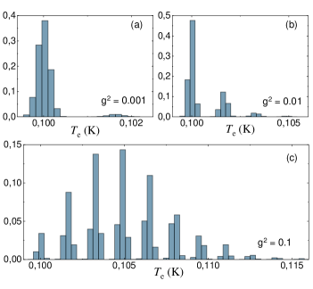
Figure 2: Temperature distributions after 10 periods of resonant driving for different values of the qubit-calorimeter coupling $g$. The distributions are obtained from histograms over $2\times 10^{5}$ realizations. The parameters used for the numerics are: $\hbar\omega_{q}=k_{\mathrm{B}}\times 1\mathrm{K}$, $V=10^{-21}$ m³, $\Sigma=2\times 10^{-9}$ WK^-5m^-3, $\gamma=1500k_{B}/(1$K), driving coupling constant $\kappa=0.05$ and the phonon temperature $T_{p}=0.1$ K.

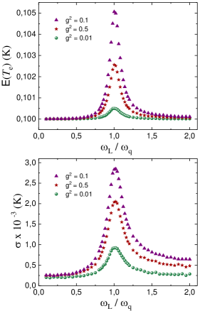
Figure 3: The first moment (top) and the standard deviation (bottom) for the distribution of the temperature after $10\frac{2\pi}{\omega_{q}}$ duration of driving. Both the mean and standard deviation peak for resonant driving and higher coupling. The parameters used for the simulations are in the caption of Figure 2.

On timescales of the order $10^{4}$ periods the qubit-temperature process exhibits convergence towards a steady state. Figure 4 illustrates this phenomenon. The (red) noisy line is a realisation of the qubit-temperature process. The smooth (blue) line is the evolution of the average temperature obtained from the analytic approximation, i.e. the evolution by the drift term of equation (26). Figure 5 shows the average value of the temperature process in the steady state versus the driving frequency, which we use as an estimate for $T_{S}$. The full line is an estimate of the same quantity as obtained by imposing the vanishing of the drift (27) and thus solving numerically the transcendental equation

$$J(X_{S})=0.$$ (44)

We notice that for $T_{e}=0$ the solution of this equation takes the form

$$T_{S}^{5}=T_{p}^{5}+\frac{g^{2}}{\Sigma\,V}\bigg{(}\hbar\,\omega^{2}_{L}\sin^{2}(\theta)$$

$$+\frac{\hbar(\omega_{L}+\nu)^{3}\sin^{4}(\theta/2)+\hbar(\omega_{L}-\nu)^{3}\cos^{4}(\theta/2)}{(\omega_{L}+\nu)\sin^{4}(\theta/2)+(\omega_{L}-\nu)\cos^{4}(\theta/2)}\bigg{)}$$ (45)

The long time behavior of the temperature is most interesting around the resonant frequency. For the rest of our numerical analysis we focus on resonant driving.

In Figure 6 we compare the value for $T_{S}$ from equation (45) (full line) with the average steady state temperature obtained from direct numerical simulations (dots). We find good agreement with the $g$ dependence predicted by (38). Furthermore, we compare the relaxation time prediction of the Ornstein–Uhlenbeck approximation with the numeric observation. The inserted plot in Figure 6 shows $\alpha=\tau_{S}^{-1}$, it demonstrates that the data are consistent with the $g$ dependence predicted by (39) and (45).

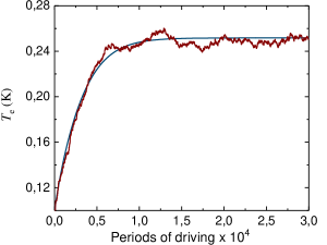
Figure 4: The long time behaviour of the temperature, the noisy (red) line is a single realisation of the qubit-temperature process given by equations (4) and (12) for $g^{2}=1/100$. The smooth (blue) line is the evolution of the average temperature by the effective temperature process (26). The parameter values are the same as in Figure 2.

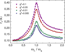
Figure 5: Mean value of the temperature in the steady state. The data come from a single realization after it reached the steady state as shown in Figure 4. The full lines are the estimate of the stationary temperature obtained from the solution of (44). The parameter values are the same as in Figure 2.

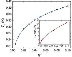
Figure 6: The mean value of the temperature in the steady state for different values of $g^{2}$ at resonant driving. The (blue) dots give an estimate for the stationary temperature obtained from the simulations. The full (blue) line is the solution obtained from the analytic approximation, the $g$ law from equation (45). (Inserted plot) The inverse of the relaxation time $\alpha=\tau_{S}^{-1}$. The (red) dots are obtained from the average of $10^{3}$ realisations of the qubit-calorimeter process by fitting to the temperature curve. The full (red) line is the $g$ law from equations (39) and (45). The parameters used for the simulations are in the caption of Figure 2.

In Figure 7 we plot the stationary value of the temperature for different values of the qubit-electron coupling $g$. We construct the histograms by sampling a single realization of the qubit-temperature process after convergence to the steady state. The full (red) line is the stationary solution of the Fokker–Planck equation (26). In Figure 7 we also report the values of the standard deviation and skewness as obtained from the numerics. In the stationary state the average value $T_{\star}$ of the temperature is close to the temperature $T_{S}$ specified by the solution of (44). The square root of the variance of the temperature process ranges from $0.004$ K to $0.005$ K.

Finally, Figure 8 shows a log-log plot of the power spectrum of the temperature process. We obtain the data by following the evolution of a single realization of the temperature process after it has reached the steady state. The spectrum exhibits a decay consistent with a fit equal to $-2$ of the slope. This is in agreement with the Ornstein–Uhlenbeck approximation (35), (36) of the drift and diffusion coefficients in the Fokker–Planck equation (26). We find in such a case the expression of the power spectrum

$$\mathcal{S}(\omega)=\frac{S^{2}(T_{S}^{2})\,\tau_{S}^{2}}{1+\omega^{2}\,\tau_{S}^{2}}$$

where $\tau_{S}$ is the relaxation time of the process.

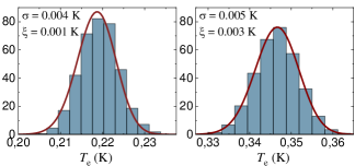
Figure 7: Probability density functions for the qubit-temperature steady state for different values of the coupling $g^{2}$. The (blue) histogram is generated from the numerical simulations. The full (red) line is the solution of equation (26). The values for the variance $\sigma=(\mathsf{E}[T_{e}(t)-\mathsf{E}(T_{e}(t))]^{2})^{1/2}$ and the skewness $\xi=(\mathsf{E}[T_{e}(t)-\mathsf{E}(T_{e}(t))]^{3})/\sigma^{3}$ obtained from the numerics are given in the figures. The parameters used for the simulations are in the caption of Figure 2.

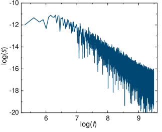
Figure 8: Power spectrum, for $g^{2}=\frac{10}{100}$. The spectrum decays with a $\omega^{-2}$ asymptotic law consistent with the Ornstein–Uhlenbeck approximation (35), (36)

VII Conclusion and Outlook

In summary, we present a theoretical model of calorimetric measurements in an integrated quantum circuit consisting of a superconducting qubit and a normal metal absorber element. The joint evolution of the population of the qubit state and the calorimeter temperature is governed by the Chapman–Kolmogorov master equation (18). Standard methods of asymptotic analysis reduce this equation to an effective Fokker–Planck equation for the probability distribution of the calorimeter temperature alone. In the asymptotic regime, we are able to make experimentally testable predictions about the dependence of statistical indicators of temperature fluctuations upon the qubit-calorimeter coupling constant.

The engineering of quantum integrated circuits of increasing tunability is in a phase of rapid development Cottet et al. (2017); Masuyama et al. (2017); Partanen et al. (2017). In particular, very recently Ronzani et al. (2018) has shown the realizability of a quantum heat valve to observe tunable heat transport between mesoscopic heat reservoirs at different temperatures. The laboratory implementation is a resonator-qubit-resonator assembly in which the qubit is capacitively embedded between two superconducting transmission lines each terminated by a normal metal resistor elements acting as mesoscopic heat reservoirs at different temperatures. The study of the heat flow in the presence of resonator elements thus appears as a natural direction towards which extend to the ideas of the present work.

VIII Acknowledgments

We warmly thank Bayan Karimi for discussions and help with the graphics. We are also gratefully acknowledge discussions with Lara Ulčakar, Antti Kupiainen and Dmitry Golubev. The work of B. D. is supported by DOMAST. B. D. and P.M-G. also acknowledge support by the Centre of Excellence in Analysis and Dynamics of the Academy of Finland. The work of J. P. P. is funded through Academy of Finland grant 312057 and from the European Union’s Horizon 2020 research and innovation programme under the European Research Council (ERC) programme (grant agreement 742559).

Appendix A Time scales in the model

Let $H(t)=H(t+\mathsf{T}_{\mathrm{p}})$ be a $\mathsf{T}_{\mathrm{p}}$-periodic self-adjoint matrix acting on $\mathbb{C}^{d}$. Floquet theory see e.g. Shirley (1965); Zel’dovich (1967); Sambe (1973); Blümel et al. (1991); Breuer and Petruccione (1997); Grifoni and Hänggi (1998); Holthaus (2015); Donvil (2018) links up solutions of the initial value problem

$$\begin{cases}\Big{(}H(t)-\imath\,\hbar\,\partial_{t}\Big{)}\psi(t)=0\\ \psi(0)=\bar{\psi}\end{cases}$$

with the spectral problem

$$\begin{cases}\Big{(}H(t)-\imath\,\hbar\,\partial_{t}\Big{)}\phi_{r,n}(t)=\epsilon_{r,n}\phi_{r,n}(t)\\ \phi_{r,n}(t+\mathsf{T}_{\mathrm{p}})=\phi_{r,n}(t).\end{cases}$$

in the Hilbert space $\mathcal{H}=\mathbb{C}^{d}\times L^{2}[0,\mathsf{T}_{\mathrm{p}}]$. Namely, if we denote by $\mathsf{F}$ the fundamental solution of (A)

$$\psi(t)=\mathsf{F}(t,0)\bar{\psi}\,,\hskip 28.45274pt\forall\,\psi\,\in\,\mathbb{C}^{d}$$ (46)

and by $\left\{\bm{e}_{r}\right\}_{r=1}^{d}$ the orthonormal basis (Floquet’s states) in $\mathbb{C}^{d}$ diagonalizing the monodromy matrix

$$\mathsf{F}(\mathsf{T}_{\mathrm{p}},0)\bm{e}_{r}=e^{-\frac{\imath\,\epsilon_{r}\,\mathsf{T}_{\mathrm{p}}}{\hbar}}\,\bm{e}_{r}$$ (47)

then, for $r=1,\dots,d$ and $n\in\mathbb{Z}$ the identities

$$\phi_{r,n}(t)=e^{\frac{\imath}{\hbar}\,\left(\epsilon_{r}+\frac{2\,\pi\,n}{\mathsf{T}_{\mathrm{p}}}\right)t}\,F_{t,0}\bm{e}_{r}$$ (48a)

$$\epsilon_{r,n}=\epsilon_{r}+\frac{2\,\pi\,n}{\mathsf{T}_{\mathrm{p}}}$$ (48b)

solve the spectral problem (A). The eigenvalues (48b) are the quasi-energies, see eq. (6) in the main text. The eigenvectors (48a) form a complete basis of $\mathcal{H}$. Setting the quantum number $n$ to zero conventionally specifies the first Brillouin zone. Note also that

$$\phi_{r,n}(0)=\bm{e}_{r}$$ (49)

for all $r,n$.

An immediate consequence of the completeness of the $\phi_{r,n}$’s is that any solution of (A) admits the expression

$$\psi(t)=\sum_{r=1}^{d}\sum_{n\in\mathbb{Z}}\phi_{r,n}(t)\,e^{-\frac{\imath\,\epsilon_{r,n}\,t}{\hbar}}\langle\langle\phi_{r,n}\,|\,\bar{\psi}\rangle\rangle$$ (50)

In (50) $\langle\langle\dots\rangle\rangle$ is the widely adopted physics notation for scalar product over $\mathcal{H}$ i.e. for any $f\,,g\,,\in\mathcal{H}$

$$\langle\langle\phi_{r,n}\,|\,\bar{\psi}\rangle\rangle\equiv\langle f\,,g\rangle_{\mathcal{H}}=\int_{0}^{\mathsf{T}_{\mathrm{p}}}\frac{\mathrm{d}t}{\mathsf{T}_{\mathrm{p}}}\langle f(t)\,|\,g(t)\rangle$$

whereas

$$\langle f(t)\,|\,g(t)\rangle=\langle f(t)\,,g(t)\rangle_{\mathbb{C}^{d}}$$

is the usual Dirac’s notation for the scalar product over $\mathbb{C}^{d}$. Finally, the insertion in (46) of the completeness relation in $\mathbb{C}^{d}$ in terms of the Floquet basis $\left\{\bm{e}_{r}\right\}_{r=1}^{d}$ combined with the definition (48a) of eigenstates of the spectral problem in the first Brillouin zone yields the identity

$$\psi(t)=\sum_{r=1}^{d}\phi_{r,0}(t)\,e^{\frac{\imath\,\epsilon_{r,0}t}{\hbar}}\,\langle\bm{e}_{r}|\bar{\psi}\rangle$$

This is the so-called Floquet’s representation of solutions of (A). As the coefficients $\langle\bm{e}_{r}|\bar{\psi}\rangle$ do not depend upon time, their absolute square value admits the interpretation of population probability of the Floquet state $r$. See Grifoni and Hänggi (1998); Holthaus (2015); Donvil (2018) for details.

Appendix B Qubit-Electron interaction

Let us consider the closed qubit-calorimeter dynamics. The Dirac’s picture Hamiltonian is

$$\tilde{H}_{qe}=\mathsf{F}^{\dagger}(t,0)\,e^{\frac{\imath\,H_{e}\,t}{\hbar}}\,H_{qe}\,e^{-\frac{\imath\,H_{e}\,t}{\hbar}}\mathsf{F}(t,0)$$ (51)

with $\mathsf{F}$ the flow (46). The Hamiltonian is the sum of tensor products of operators independently acting on the Hilbert space of the qubit and of the electrons. The operator acting on the qubit Hilbert space always admits the representation

$$\mathsf{F}^{\dagger}(t,0)(\sigma_{+}+\sigma_{-})\mathsf{F}(t,0)$$

$$=\sum_{r,s=0}^{1}e^{\imath\frac{\epsilon_{r,0}-\epsilon_{s,0}}{\hbar}t}|\phi_{r,0}(0)\rangle\tilde{D}_{r,s}(t)\langle\phi_{s,0}(0)|$$

where

$$\tilde{D}_{r,s}(t)=\langle\phi_{r,0}(t)|\sigma_{+}+\sigma_{-}|\phi_{s,0}(t)\rangle$$

The completeness for any $t$ in $\mathbb{C}^{2}$ of the Floquet basis immediately implies

$$\tilde{D}_{0,0}(t)=-\tilde{D}_{1,1}(t)$$

Furthermore, $\tilde{D}_{r,s}(t)$ is a $2\,\pi/\omega_{L}$ periodic function the Fourier series whereof is amenable to the form

$$\tilde{D}_{r,s}(t)=\sum_{n\in\mathbb{Z}}e^{\imath\,\omega_{L}\,n\,t}D_{r,s,n}$$ (52)

with $D_{r,n,s}$ defined by (7). The advantage of the Floquet representation is to couch the time dependence of the Dirac picture Hamiltonian into the form of a sum over purely oscillating exponentials as in the case of bipartite isolated systems.

In the weak coupling scaling limit, at leading order we consider transition occurring for non-vanishing matrix elements of (51) satisfying the resonance condition

$$\eta_{k}-\eta_{l}=\epsilon_{r,0}-\epsilon_{s,0}+n\,\hbar\,\omega_{L}$$

where $\eta_{k}$, $\eta_{l}$ are energy levels of the free electron Hamiltonian. These considerations Breuer and Petruccione (2002) fix the form of the Lindblad operators (5).

Finally, to explain the Bose–Einstein distribution appearing in (11), we observe that the emission of $\hbar\omega$ energy from the qubit to the calorimeter occurs with rate

$$\mathcal{R}(\omega)\propto$$ (53)

$$\frac{g^{2}}{N^{2}}\sum_{i\,j}f_{T_{e}}(\eta_{i})\left(1-f_{T_{e}}(\eta_{j})\right)\frac{\sin\big{(}\frac{\eta_{i}-\eta_{j}-\hbar\omega}{\hbar}t\big{)}}{\eta_{i}-\eta_{j}-\hbar\omega}$$

where $t$ is the duration of the interaction, $\eta_{i}$ denotes the $i$-th electron energy level and

$$f_{T_{e}}(\eta)=\frac{1}{e^{(\eta-\mu)/(k_{B}\,T_{e})}+1}.$$ (54)

is the Fermi–Dirac distribution at temperature $T_{e}$. In the large $N$ limit, we approximate the double sum over the electron energy levels with a double integral. The integrand is then amenable to further simplifications. The weak coupling scaling limit yields

$$\frac{\sin\big{(}\frac{\eta_{i}-\eta_{j}-\hbar\omega}{\hbar}t\big{)}}{\eta_{i}-\eta_{j}-\hbar\omega}\overset{t\uparrow\infty}{\to}\,\hbar\,\pi\,\delta\left(\eta_{i}-\eta_{j}-\hbar\omega\right)$$

Moreover, the low temperature limit permits to set the energy density of states to a constant value in the region where the integrand is sensibly different from zero Ingold and Nazarov (1992). Finally we can extend the range of integration to the full real axis. The upshot is

$$\mathcal{R}(\omega)\propto g^{2}\int_{\mathbb{R}}\mathrm{d}E\,f_{T_{e}}(E)\bigg{(}1-f_{T_{e}}(E-\hbar\,\omega)\bigg{)}$$

We avail us of the identity

$$f_{T_{e}}(E)\bigg{(}1-f_{T_{e}}(E-\hbar\,\omega)\bigg{)}$$ (55)

$$=\frac{e^{\hbar\,\omega/(K_{B}T_{e})}}{e^{\hbar\,\omega/(K_{B}T_{e})}-1}\bigg{(}f_{T_{e}}(E-\hbar\,\omega)-f_{T_{e}}(E)\bigg{)}$$

to couch the integral into the form

$$\mathcal{R}(\omega)\approx\frac{g^{2}\,e^{\hbar\omega/(k_{B}T_{e})}}{e^{\hbar\omega/(k_{B}T_{e})}-1}\,\int_{\mathbb{R}}\mathrm{d}E\,(f(E-\hbar\,\omega)-f(E))$$ (56)

and upon noticing that

$$\frac{\mathrm{d}\mathcal{R}}{\mathrm{d}\omega}(\omega)\approx-\frac{g^{2}\,e^{\hbar\omega/(k_{B}T_{e})}}{e^{\hbar\omega/(k_{B}T_{e})}-1}\,\int_{\mathbb{R}}\mathrm{d}E\,\frac{1}{\hbar}\frac{\mathrm{d}}{\mathrm{d}E}f(E-\hbar\,\omega)$$

we finally get into

$$\mathcal{R}(\omega)\approx\frac{g^{2}\,\hbar\,\omega\,e^{\hbar\omega/(k_{B}T_{e})}}{e^{\hbar\omega/(k_{B}T_{e})}-1}$$

Appendix C Electron-Phonon interaction

For reader convenience, we summarize here the calculation of the first two moments of the energy flux between the phonon and the electron reservoirs. We perform the calculation under the following hypotheses Wellstood et al. (1994)

1. The electron gas

   $$H_{e}=\sum_{k}\eta_{k}\,c_{k}^{\dagger}\,c_{k}$$

   is initially at equilibrium at a uniform temperature $T_{e}\ll T_{F}$ with $T_{F}$ the Fermi temperature. The energy of an electron having wave-number $\bm{k}$ is

   $$\eta_{k}=\frac{\hbar k^{2}}{2\,m}\,,\hskip 28.45274ptk=\|\bm{k}\|$$

2. The phonon gas

   $$H_{p}=\sum_{k}\hbar\,\omega_{k}\,b_{k}^{\dagger}\,b_{k}$$

   is initially at equilibrium with an uniform temperature $T_{p}\,\ll\,T_{D}$ with $T_{D}$ the Debye temperature Ashcroft and Mermin (1976). In this temperature limit, phonons obey a linear dispersion relation

   $$\omega_{k}=v_{s}\,k$$

   $v_{s}$ the speed of sound and $k=\|\bm{k}\|$ for $\bm{k}$ the phonon wavelength.

3. The interaction between the phonons and the electrons in the material is given by

   $$H_{ep}=\kappa\sum_{\bm{k},\bm{q}}\omega_{q}^{1/2}\Big{(}\,c^{\dagger}_{\bm{k}}\,c_{\bm{k}-\bm{q}}\,b_{\bm{q}}+c^{\dagger}_{\bm{k}}\,c_{\bm{k}-\bm{q}}\,b^{\dagger}_{\bm{q}}\Big{)}$$ (57)

   The sum in (57) ranges over energies sufficiently close to the Fermi surface.

4. Scattering processes with out-coming phonons with wave numbers in a different Brillouin zone than incoming ones, are negligible (no “umklapp” Ashcroft and Mermin (1976)).

5. The dimensions of the metal are much longer than the average phonon wavelength. This means that sums over wave numbers can be replaced by integrals over approximately constant density of states $D$ for phonons and $N$ for electrons.

Following Pekola and Karimi (2018) we evaluate the average heat current in terms of the current operator $\mathfrak{J}$ defined by

$$J=\frac{\mathrm{d}}{\mathrm{d}t}\operatorname{Tr}\left(\frac{H_{e}-H_{p}}{2}\,\bm{\rho}_{t}\right)\equiv\operatorname{Tr}(\mathfrak{J}\,\bm{\rho}_{t})$$ (58)

Here $\bm{\rho}_{t}$ is the state operator of the phonon-electron system in Schrödinger’s picture. The Liouville–von Neumann equation yields

$$\mathfrak{J}=-\frac{\imath\,\kappa}{2\,\hbar}\sum_{k,q}\omega_{q}^{1/2}\,\Omega_{k,q}\,(a^{\dagger}_{\bm{k}}\,a_{\bm{k}-\bm{q}}\,c_{\bm{q}}-a^{\dagger}_{\bm{k}-\bm{q}}\,a_{\bm{k}}\,c^{\dagger}_{\bm{q}})$$

with $\Omega_{k,q}=\omega_{q}+\eta_{k}-\eta_{\|\bm{k}-\bm{q}\|}$. Turning to Dirac’s picture and writing $\tilde{\mathfrak{J}}$ for heat current in said picture, within leading order accuracy in the weak coupling limit Breuer and Petruccione (2002) the average heat current

$$J=\imath\operatorname{Tr}\int_{0}^{t}\mathrm{d}s[\tilde{H}_{pe}(s),\tilde{\mathfrak{J}}(t)]\bm{\rho}_{0}+\mathrm{h.o.t.}$$

is amenable Kaganov et al. (1957); Wellstood et al. (1994) to the difference $J=J_{a}-J_{e}$ of two terms physically corresponding to the absorption and the emission of one phonon by the electron gas. Under the aforementioned hypotheses i-v, the absorption term is Wellstood et al. (1994)

$$J_{a}=C\int\mathop{}\!\mathrm{d}^{3}q\,n_{T_{p}}(\omega_{q})\,\Big{(}n_{T_{e}}(\omega_{q})+1\Big{)}\,\hbar^{2}\omega_{q}^{2}\,I(\omega_{q})$$ (59)

whilst emission is

$$J_{e}=C\int\mathop{}\!\mathrm{d}^{3}q\,\Big{(}n_{T_{p}}(\omega_{q})+1\Big{)}\,n_{T_{e}}(\omega_{q})\,\hbar^{2}\omega_{q}^{2}\,I(\omega_{q})$$ (60)

with

$$I(\omega_{q})=$$ (61)

$$\int\mathop{}\!\mathrm{d}^{3}k\Big{(}f_{T_{e}}(\eta_{k-q})-f_{T_{e}}(\eta_{k})\big{)}\,\delta(\eta_{k}-\eta_{\|\bm{k}-\bm{q}\|}-\hbar\omega_{q})$$

In writing (59), (60) we defined $C=2\,\pi\,D\,N\,\kappa^{2}\hbar^{-1}$ and we took advantage of the explicit form of the Fermi–Dirac (54) and Bose–Einstein distributions

$$n_{T_{p}}(\omega_{q})=\frac{1}{e^{\hbar\omega_{q}/(k_{B}T_{p})}-1}$$

and of the identity (55). We also exploited the fact that the Dirac delta in (61) fixes the difference $\eta_{\|\bm{k}-\bm{q}\|}-\eta_{k}=\omega_{q}$ to a $\bm{k}$ independent value. The integral (61) is most conveniently evaluated in polar coordinates

$$I(\omega_{q})=$$

$$2\,\pi\,\int_{0}^{\infty}\mathop{}\!\mathrm{d}k\,k^{2}\int_{-1}^{1}\mathop{}\!\mathrm{d}z\,\iota(k,z;\omega_{q})\,\delta\left(\hbar\,\omega_{q}+\frac{\omega_{q}\,k\,z}{m\,v_{s}}-\eta_{q}\right)$$

where $z$ is the angle between $\bm{k}$ and $\bm{q}$, and

$$\iota(k,z;\omega_{q})=$$

$$f_{T_{e}}\left(\eta_{k}+\eta_{q}-\frac{\omega_{q}\,k\,z}{m\,v_{s}}\right)-f_{T_{e}}(\eta_{k})$$

Upon evaluating the integral over $z$ we find

$$I(\omega_{q})=$$

$$\frac{2\,\pi\,m^{2}\,v_{s}}{\hbar^{4}\omega_{q}}\int_{E_{min}}^{+\infty}\mathop{}\!\mathrm{d}E\,\Big{(}f_{T_{e}}(E-\hbar\omega_{q})-f_{T_{e}}(E)\Big{)}$$

having set $E=\frac{\hbar^{2}|k|^{2}}{2m}$ and

$$E_{min}=\frac{\hbar^{2}}{2m}\left(\frac{\omega_{q}}{2\,v_{s}}+\frac{v_{s}m}{\hbar}\right)^{2}$$

The remaining integrand is peaked around $\mu$. Under our working hypotheses (see Kaganov et al. (1957); Wellstood et al. (1994)), the chemical potential satisfies $\mu\gg\frac{\hbar^{2}}{2m}(\frac{q}{2}+\frac{v_{s}m}{\hbar})^{2}$ allowing us to write

$$I(\omega_{q})\approx$$

$$\frac{2\,\pi\,m^{2}\,v_{s}}{\hbar^{4}\omega_{q}}\int_{-\infty}^{+\infty}\mathop{}\!\mathrm{d}E\,\Big{(}f_{T_{e}}(E-\hbar\omega_{q})-f_{T_{e}}(E)\Big{)}$$

whence

$$I(\omega_{q})\approx\frac{2\,\pi\,m^{2}\,v_{s}}{\hbar^{3}}$$

We thus get into

$$J=J_{a}-J_{e}=$$ (62)

$$\frac{2\,\pi m^{2}\,C\,v_{s}}{\hbar^{3}}\int\mathop{}\!\mathrm{d}^{3}q\,\Big{(}n_{T_{p}}(\omega_{q})-n_{T_{e}}(\omega_{q})\Big{)}\,\omega_{q}^{2}$$

The remaining integral is the proportional to the difference between two averages with respect to the Bose–Einstein distribution. It can be evaluated by standard techniques see e.g. Ashcroft and Mermin (1976). The final result is

$$J=\Sigma\,V\,(T_{p}^{5}-T_{e}^{5})$$ (63)

where $V$ is the volume of the metal and Pekola and Karimi (2018)

$$\Sigma=\frac{12\,\kappa^{2}\,\zeta(5)\,m\,k_{\mathrm{B}}^{5}}{\pi\,k_{F}\,v_{s}^{2}\,\hbar^{6}}$$ (64)

with $\zeta$ the Riemann zeta functions an $k_{F}$ the Fermi momentum. The definition of $\Sigma$ hinges upon setting $D=V/(2\pi)^{3}$ for the phonon density of states

The evaluation of current correlation function

$$\mathcal{C}_{t}=\operatorname{Tr}U^{\dagger}_{t}\mathfrak{J}U_{t}\mathfrak{J}\bm{\rho}_{0}$$

with

$$U_{t}=\exp\left(-\imath\frac{H_{e}+H_{p}+H_{pe}}{\hbar}t\right)$$

proceeds along the same lines as above. We refer to Pekola and Karimi (2018) for details. Within leading accuracy and at $T_{e}=T_{p}$ we get into

$$\int_{-\infty}^{\infty}\mathrm{d}t\,\mathcal{C}_{t}=10\,\Sigma\,V\,k_{B}\,T_{p}^{6}.$$ (65)

We use this result to weight Brownian fluctuations in the temperature process.

Appendix D Master equation

In this Appendix we derive the master equation (18). We start by writing the probability (17) in the form

$$P_{r}(X,t)=\mathsf{E}\Big{(}|\langle\bm{e}_{r}|\psi(t)\rangle|^{2}\delta(\xi(t)-X)\Big{)}$$ (66)

where $\mathsf{E}(.)$ is the average and $\bm{e}_{r}=\phi_{r,0}(0)$. We find the master equation by evaluating

$$\mathop{}\!\mathrm{d}P_{r}(X,t)=\mathsf{E}\mathop{}\!\mathrm{d}\Big{(}|\langle\bm{e}_{r}|\psi(t)\rangle|^{2}\delta(\xi(t)-X)\Big{)}$$ (67)

Let us call $f(\psi_{t},\psi^{*}_{t},\xi)=|\langle\bm{e}_{r}|\psi\rangle|^{2}\delta(\xi-X)$. The differential of $f$ is

$$\mathop{}\!\mathrm{d}f(\psi,\psi^{*},\xi)\equiv$$

$$f(\psi+\mathop{}\!\mathrm{d}\psi,\psi^{*}+\mathop{}\!\mathrm{d}\psi^{*},\xi+\mathop{}\!\mathrm{d}\xi)-f(\psi,\psi^{*},\xi)=$$

$$\sum_{\begin{subarray}{c}p=1\\ p=k_{1}+k_{2}+k_{3}\end{subarray}}^{\infty}\frac{(\mathop{}\!\mathrm{d}\xi)^{k_{1}}(\mathop{}\!\mathrm{d}\psi^{*})^{k_{2}}(\mathop{}\!\mathrm{d}\psi)^{k_{3}}}{k_{1}!k_{2}!k_{3}!}\partial_{\xi}^{k_{1}}\partial_{\psi^{*}}^{k_{2}}\partial_{\psi}^{k_{3}}f(\psi,\psi^{*},\xi)$$

We then use (4) and (16) to express the differentials $\mathrm{d}\psi$, $\mathrm{d}\psi^{*}$ and $\mathrm{d}\xi$, in terms of the time differential $\mathrm{d}t$ and the increments $\mathrm{d}w$ and $\mathrm{d}\nu$ of Wiener and Poisson processes. The rules of stochastic calculus, see e.g. Jacobs (2010), impose $\mathop{}\!\mathrm{d}w^{2}(t)=t$, $\mathop{}\!\mathrm{d}w(t)\mathop{}\!\mathrm{d}\nu_{r,n}(t)=0$ and $\mathop{}\!\mathrm{d}\nu_{r,n}(t)\mathop{}\!\mathrm{d}\nu_{r^{\prime},n^{\prime}}(t)=\delta_{r,r^{\prime}}\delta_{n,n^{\prime}}\mathop{}\!\mathrm{d}\nu_{r,n}(t)$. We thus get into the Itô–Poisson stochastic differential

$$\mathop{}\!\mathrm{d}f(\psi,\psi^{*},\xi)=\mathcal{L}_{\xi}^{\dagger}f(\psi,\psi^{*},\xi)\mathop{}\!\mathrm{d}t$$ (68)

$$+\frac{\sqrt{10\Sigma Vk_{B}}T^{3}_{p}}{\gamma}\partial_{\xi}f(\psi,\psi^{*},\xi)\mathop{}\!\mathrm{d}w(t)$$

$$-\frac{\imath}{\hbar}\Big{(}\,G(\psi)\partial_{\psi}-G^{*}(\psi)\partial_{\psi^{*}}\Big{)}f(\psi,\psi^{*},\xi)\mathop{}\!\mathrm{d}t$$

$$+\mathrm{d}_{jump}f(\psi,\psi^{*},\xi)$$

$\mathcal{L}^{\dagger}$ is the $\mathbb{L}^{(2)}$ adjoint of (19) with respect to the Lebesgue measure

$$\mathcal{L}_{\xi}^{\dagger}f=\frac{\Sigma\,V}{N\,\gamma}(T^{5}_{p}-\xi^{5/2})\partial_{\xi}f+\frac{10\Sigma Vk_{B}T^{6}_{p}}{2\,N^{2}\,\gamma^{2}}\partial^{2}_{\xi}f$$

Furthermore we can couch

$$-\frac{\imath}{\hbar}\Big{(}G(\psi)\partial_{\psi}-G^{*}(\psi)\partial_{\psi^{*}}\Big{)}\,|\left\langle\bm{e}_{r}\right|\psi\rangle|^{2}\delta(\xi-X)=$$

$$\sum_{\begin{subarray}{c}|s|\leq 1\\ |n|\leq\mathcal{N}\end{subarray}}\Gamma(\omega_{s,n},\xi)\|A_{s,n}\psi\|^{2}|\langle\bm{e}_{r}|\psi\rangle|^{2}\delta(\xi-X)$$

$$-\sum_{\begin{subarray}{c}|s|\leq 1\\ |n|\leq\mathcal{N}\end{subarray}}\Gamma(\omega_{s,n},\xi)\operatorname{Re}\langle\bm{e}_{r}|A^{\dagger}_{s,n}A_{s,n}|\psi\rangle\langle\psi|\bm{e}_{r}\rangle\delta(\xi-X)$$

into the form

$$-\imath\,\hbar\Big{(}G(\psi)\partial_{\psi}-G^{*}(\psi)\partial_{\psi^{*}}\Big{)}\|\left\langle\bm{e}_{r}\right|\psi\rangle\|^{2}\delta(\xi-X)=$$ (69)

$$\sum_{\begin{subarray}{c}|s|\leq 1\\ |n|\leq\mathcal{N}\end{subarray}}\Gamma(\omega_{s,n},\xi)\,\|A_{s,n}\psi\|^{2}\langle\bm{e}_{r}|\psi\rangle|^{2}\delta(\xi-X)\mathop{}\!\mathrm{d}t$$

$$-\sum_{\begin{subarray}{c}r^{\prime}=0,1\\ |n|\leq\mathcal{N}\end{subarray}}\mathcal{G}_{r^{\prime},r,n}(\xi)\,\langle\bm{e}_{r}|\psi\rangle|^{2}\delta(\xi-X)\mathop{}\!\mathrm{d}t$$

having used (5), (7) to derive

$$\sum_{|s|\leq 1}\Gamma(\omega_{s,n},\xi)\operatorname{Re}(\langle\bm{e}_{r}|A^{\dagger}_{s,n}A_{s,n}|\psi\rangle\langle\psi,\bm{e}_{r}\rangle)$$

$$=\Gamma(\omega_{0,n},\xi)|D_{1,1,n}|^{2}\langle\bm{e}_{r}|\psi\rangle$$

$$+\Big{(}\delta_{r,0}\Gamma(\omega_{1,n},\xi)\,|D_{1,0,n}|^{2}+\delta_{r,1}\Gamma(\omega_{-1,n},\xi)\,|D_{0,1,n}|^{2}\Big{)}\langle\bm{e}_{r}|\psi\rangle$$

and the definition (21) for $\mathcal{G}_{r^{\prime},r,n}(\xi)$. The last term on the right hand side of (68) is purely due to jumps

$$\mathrm{d}_{jump}f(\psi,\psi^{*},\xi)=-\sum_{\begin{subarray}{c}s=-1\\ |n|\leq\mathcal{N}\end{subarray}}^{1}\mathrm{d}\nu_{s,n}f(\psi,\psi^{*},\xi)$$

$$+\sum_{\begin{subarray}{c}|s|\leq 1\\ |n|\leq\mathcal{N}\end{subarray}}\mathrm{d}\nu_{s,n}f\left(\frac{(A_{s,n}\psi)}{\|A_{s,n}\psi\|},\frac{(A_{s,n}\psi)^{*}}{\|A_{s,n}\psi\|},\xi+\frac{\hbar\omega}{N\,\gamma}\right)$$

or more explicitly

$$\mathrm{d}_{jump}f(\psi,\psi^{*},\xi)=$$ (70)

$$-\sum_{\begin{subarray}{c}s=-1\\ |n|\leq\mathcal{N}\end{subarray}}^{1}\mathrm{d}\nu_{s,n}\,\langle\bm{e}_{r}|\psi\rangle|^{2}\delta(\xi-X)\mathop{}\!\mathrm{d}t$$

$$+\sum_{\begin{subarray}{c}s=-1\\ |n|\leq\mathcal{N}\end{subarray}}^{1}\mathrm{d}\nu_{s,n}\,\frac{|\langle\bm{e}_{r}|A_{s,n}|\psi\rangle|^{2}}{\|A_{s,n}\psi\|^{2}}\delta\left(\xi+\frac{\hbar\omega_{s,n}}{N\,\gamma}-X\right)$$

Taking the expectation value of (68) brings about several simplifications. To start with, the term proportional to the increment of the Wiener vanishes owing to the Itô prescription Jacobs (2010) whereas the identity

$$\mathsf{E}\Big{(}|\langle\bm{e}_{r}|\psi_{t}\rangle|^{2}\mathcal{L}_{\xi}\delta(\xi-X)\Big{)}=\mathcal{L}_{X}P_{r}(X,t)$$

holds in consequence of the properties of the Dirac-$\delta$ distribution. By (10), the expectation value of (70) yields

$$\mathsf{E}\Big{(}\mathrm{d}_{jump}f(\psi,\psi^{*},\xi)\Big{)}=$$

$$-\sum_{\begin{subarray}{c}s=-1\\ |n|\leq\mathcal{N}\end{subarray}}^{1}\mathsf{E}\Big{(}\Gamma(\omega_{s,n},\xi)\,\|A_{s,n}\psi\|^{2}\langle\bm{e}_{r}|\psi\rangle|^{2}\delta(\xi-X)\Big{)}\mathop{}\!\mathrm{d}t$$

$$+\sum_{\begin{subarray}{c}r^{\prime}=0,1\\ |n|\leq\mathcal{N}\end{subarray}}\mathsf{E}\left(\mathcal{G}_{r,r^{\prime},n}(\xi)\,\langle\bm{e}_{r^{\prime}}|\psi\rangle|^{2}\delta\left(\xi+\frac{\hbar\,\omega_{r-r^{\prime},n}}{N\,\gamma}-X\right)\right)\mathop{}\!\mathrm{d}t$$

having also used (5) to evaluate

$$|\langle\bm{e}_{r}|A_{s,n}|\psi\rangle|^{2}=\delta_{s,0}|D_{1,1,n}|^{2}\,|\langle\bm{e}_{r}|\psi\rangle|^{2}$$

$$+(\delta_{s,1}\delta_{r,1}+\delta_{s,-1}\delta_{r,0})|D_{r,r-s,n}|^{2}|\langle\bm{e}_{r-s}|\psi\rangle|^{2}$$

and the definition (21) of the rates of the master equation. If we contrast this last result with (69) we notice that the first term on the right hand side of both expression mutually cancel. Gathering all non vanishing contributions, and recalling the definitions (20), (21) we obtain

$$\frac{\mathrm{d}}{\mathrm{d}t}P_{r}(X,t)=\mathcal{L}_{X}P_{r}(X,t)$$ (71)

$$+\sum_{\begin{subarray}{c}r^{\prime}=0,1\\ |n|\leq\mathcal{N}\end{subarray}}\mathcal{G}_{r,r^{\prime},n}\left(X-\frac{\hbar\,\omega_{r-r^{\prime},n}}{N\,\gamma}\right)\,P_{r^{\prime}}\left(X-\frac{\hbar\,\omega_{r-r^{\prime},n}}{N\,\gamma},t\right)$$

$$-\sum_{\begin{subarray}{c}r^{\prime}=0,1\\ |n|\leq\mathcal{N}\end{subarray}}\mathcal{G}_{r^{\prime},r,n}(X)\,P_{r}(X,t)$$

which is (18).

Appendix E Temperature process

We analyze here the perturbative solution of (23) up to order $O(\varepsilon^{2})$.

Order $\varepsilon^{0}$

The lowest order satisfies

$$\sum_{s=0}^{1}\bigg{(}\mathds{G}^{(0)}_{r,s}(X)Q_{s}(X)-\mathds{G}^{(0)}_{s,r}(X)Q_{r}(X)\bigg{)}=0$$ (72a)

$$Q_{0}(X)+Q_{1}(X)=1$$ (72b)

It is helpful to represent the condition (72a) in the matrix form

$$\mathds{M}(X)\bm{Q}(X)=0$$

where $\mathds{M}$ is the two dimensional matrix

$$\mathds{M}(X)=\begin{bmatrix}-\mathds{G}^{(0)}_{1,0}(X)&\mathds{G}^{(0)}_{0,1}(X)\\ \mathds{G}^{(0)}_{1,0}(X)&-\mathds{G}^{(0)}_{0,1}(X)\end{bmatrix}$$ (73)

As required by probability conservation, columns of (73) add up to zero. The solution of (72a) is the thermal state for the qubit at temperature $T=\sqrt{X}$

$$Q_{r}(X)=\frac{\mathds{G}^{(0)}_{r,1-r}(X)}{\mathds{G}^{(0)}_{1,0}(X)+\mathds{G}^{(0)}_{0,1}(X)}\,\hskip 14.22636ptr=0,1$$ (74)

which in vector notation is (24).

Order $\varepsilon$

The first order correction solves

$$\sum_{s=0}^{1}\mathds{M}_{rs}(X)\bar{P}^{(1)}_{s}(X,t)=-\dot{F}^{(0)}(X,t)Q_{r}(X)$$

$$+\sum_{s=0}^{1}\big{(}\mathcal{L}_{X}^{(1)}\delta_{rs}+\partial_{X}\mathds{G}^{(1)}_{rs}(X)\big{)}\,Q_{s}(X)\,F^{(0)}(X,t)$$ (75)

By Fredholm’s alternative Pavliotis and Stuart (2008), linear non-homogeneous equations of generated by an Hilbert’s expansion are solvable if the non-homogeneous term is orthogonal to the kernel of the adjoint $\mathds{M}^{\dagger}$ of the leading order linear operator $\mathds{M}$ Pavliotis and Stuart (2008).

The spectral analysis of $\mathds{M}$ shows that the dual zero mode equation

$$\mathds{M}^{\dagger}\bm{Z}=0$$

yields (29). We choose the normalization of $\bm{Z}$ such that (72b) can be re-written as the scalar product

$$\langle\bm{Z}|\bm{Q}\rangle\equiv\sum_{r=0}^{1}Z_{r}Q_{r}(X)=1$$ (76)

The quantity $\lambda$ introduced in (31) is the non vanishing eigenvalue of $\mathds{M}$, $\mathds{M}^{\dagger}$. The corresponding left eigenvector is

$$\mathds{M}^{\dagger}(X)\bm{Q}^{\perp}(X)=\lambda(X)\bm{Q}^{\perp}(X)$$ (77a)

$$\bm{Q}^{\perp}(X)=\frac{1}{\lambda(X)}\begin{bmatrix}\mathds{G}^{(0)}_{1,0}\\ -\mathds{G}^{(0)}_{0,1}\end{bmatrix}=\mathds{J}\bm{Q}$$ (77b)

with $\mathds{J}$ defined by (32), so that

$$\sum_{r=0}^{1}Q^{\perp}_{r}(X)Q_{r}(X)=\langle\mathds{J}\bm{Q}|\bm{Q}\rangle=0$$

as $\mathds{J}$ is real antisymmetric. The right eigenvector is

$$\mathds{M}(X)\bm{V}(X)=\lambda(X)\bm{V}(X)$$ (78b)

$$\bm{V}(X)=\begin{bmatrix}-1\\ 1\end{bmatrix}=\mathds{J}\,\bm{Z}$$

normalized so that

$$\sum_{r=0}^{1}Q^{\perp}_{r}(X)V_{r}(X)=1$$

Finally we notice that for any $X$ we can write the completeness relation in $\mathbb{C}^{2}$ of left and right eigenvectors of $\mathds{M}$ as

$$\mathds{1}=|\bm{Q}\rangle\langle\bm{Z}|+|\bm{V}\rangle\langle\bm{Q}^{\perp}|$$ (79)

Projecting (E) onto the zero mode (29), yields the solvability condition

$$\dot{F}^{(0)}(X,t)=$$ (80)

$$\mathcal{L}_{X}^{(1)}\,F^{(0)}(X,t)+\partial_{X}\jmath^{(1)}(X)\,F^{(0)}(X,t)$$

with $\jmath^{(1)}$ respectively defined by (25) and (30a). This equation determines $F^{(0)}$. From the probabilistic point of view $F^{(0)}$ is within leading order approximation the probability density for the squared temperature $X$. From the geometric slant, $F^{(0)}$ is, within the same accuracy, the coordinate in the $\bm{Q}$, $\bm{V}$ basis of the solution of (23):

$$F^{(0)}=\langle\bm{Z}|\bm{P}^{(0)}\rangle$$

The projection of (E) onto (77b) yields

$$\lambda\sum_{r=0}^{1}Q^{\perp}_{r}\bar{P}_{r}^{(1)}=\sum_{r,s=0}^{1}Q^{\perp}_{r}(\mathcal{L}_{X}^{(1)}\delta_{rs}+\partial_{X}\mathds{G}^{(1)}_{rs})Q_{s}\,F^{(0)}$$

This equation yields the component along $\bm{V}$ of

$$\bm{\bar{P}}^{(1)}=F^{(1)}\,\bm{Q}+F_{V}^{(1)}\bm{V}$$

where

$$F^{(1)} = \langle\bm{Z}|\bm{P}^{(1)}\rangle=\bar{P}^{(1)}_{0}(X,t)+\bar{P}^{(1)}_{1}(X,t)$$

$$F_{V}^{(1)} = \frac{\langle\bm{Q}^{\perp}|\bm{P}^{(1)}\rangle}{\lambda}$$

$$= \frac{1}{\lambda}\left\langle\bm{Q}^{\perp}\big{|}(\mathcal{L}_{X}^{(1)}\bm{Q})\,F^{(0)}+\partial_{X}(\mathds{G}^{(1)}\bm{Q}\,F^{(0)})\right\rangle$$

Order $\varepsilon^{2}$

The second order equation is

$$\sum_{s=0}^{1}\mathds{M}_{rs}\bar{P}^{(2)}_{s}=-\partial_{t}\bar{P}^{(1)}_{r}+\mathcal{L}_{X}^{(1)}\bar{P}^{(1)}_{r}$$

$$+\sum_{s=0}^{1}\partial_{X}(\mathds{G}^{(1)}_{rs}P^{(1)}_{s})+\mathcal{L}_{X}^{(2)}Q_{r}F^{(0)}+\sum_{s=0}^{1}\partial_{X}(\mathds{G}^{(2)}_{rs}Q_{s}F^{(0)})$$

The solvability condition is

$$\partial_{t}F^{(1)}=\mathcal{L}_{X}^{(1)}F^{(1)}+\mathcal{L}_{X}^{(2)}F^{(0)}$$

$$+\sum_{r,s=0}^{1}\left(\partial_{X}\mathds{G}^{(1)}_{rs}P^{(1)}_{s}+\frac{1}{2}\partial_{X}^{2}\mathds{G}^{(2)}_{rs}Q_{s}\,F^{(0)}\right)$$

or equivalently in the scalar product notation

$$\partial_{t}F^{(1)} = \mathcal{L}_{X}^{(1)}F^{(1)}+\mathcal{L}_{X}^{(2)}F^{(0)}+\partial_{X}\langle\bm{Z}|\mathds{G}^{(1)}\bm{Q}\rangle\,F^{(1)}$$ (82)

$$+ \partial_{X}\frac{\langle\bm{Z}|\mathds{G}^{(1)}\bm{V}\rangle\langle\bm{Q}^{\perp}|(\mathcal{L}_{X}^{(1)}\bm{Q})\rangle}{\lambda}\,F^{(0)}$$

$$+ \partial_{X}\frac{\langle\bm{Z}|\mathds{G}^{(1)}\bm{V}\rangle\langle\bm{Q}^{\perp}|\partial_{X}(\mathds{G}^{(1)}\bm{Q}\,F^{(0)})\rangle}{\lambda}$$

$$+ \frac{1}{2}\partial_{X}^{2}\langle\bm{Z}|\mathds{G}^{(2)}\bm{Q}\rangle\,F^{(0)}$$

We get into

$$\partial_{t}F^{(1)}=\mathcal{L}_{X}^{(1)}F^{(1)}+\mathcal{L}_{X}^{(2)}F^{(0)}$$ (83)

$$-\partial_{X}\left(\sum_{i=1}^{2}\jmath^{(i)}\,F^{(i)}\right)+\frac{1}{2}\partial_{X}^{2}\left(S\,F^{(0)}\right)$$

where $\jmath^{(1)}$ and $\jmath^{(2)}$ are respectively specified by (30a), (30b) and the diffusion coefficient $S$ is defined by equation (33) in the main text.

Order $O(\varepsilon^{2})$ accuracy approximation

Let us now define $F(X,t)=F_{0}(X,t)+\varepsilon F_{1}(X,t)$ then summing equations (80) and $\varepsilon$ times (83) reconstruct within $O(\varepsilon)$ accuracy the Fokker-Planck equation (26).

Positivity of the diffusion coefficient

By construction the matrix $\mathds{G}^{(2)}$ has positive components. Hence

$$\Delta^{(1)}(X)\,>\,0$$

because it is the sum of positive addends. To prove that

$$\Delta^{(2)}(X)\,>\,0$$

we observe that the two dimensional matrix $\mathds{G}_{1}$ has the form

$$\mathds{G}^{(1)}=\begin{bmatrix}m_{1}&m_{2}\\ -m_{3}&m_{1}\end{bmatrix}$$

for $m_{i}\,\geq\,0$ and $i=1,2,3$. Hence

$$\Delta^{(2)}(X) = 2\,\frac{\langle\bm{Z}|\mathds{G}^{(1)}\mathds{J}\bm{Z}\rangle\langle\bm{Q}^{\perp}|\mathds{G}^{(1)}\mathds{J}^{-1}\bm{Q}^{\perp}\rangle}{\lambda}$$

$$= 2\frac{(\sum_{r=0}^{1}Z_{r}^{2}m_{r})(\sum_{s=0}^{1}(Q^{\perp}_{s})^{2}m_{s})}{|\lambda|}\,\geq\,0$$