On Hyperparameter Search
in Cluster Ensembles

1 Introduction

Hyperparameter optimization for supervised learning models is classically accomplished with respect to an external accuracy measure or objective function defined on behalf of either class labels or regression values. Different models and outcomes of different hyperparameter configurations can therefore be scored and compared easily. The actual hyperparameter optimization methods then depend on the chosen model and range from random search methods (see for example Bergstra and Bengio 2012) over brute force grid evaluation to gradient descent variants and greedy methods on the hyperparameter space (Kingma and Ba 2014). However, the situation in unsupervised learning tasks such as data clustering is generally different due to the lack of a universal interpretation of the validity of a model. Over the years, various approaches to define clustering quality measures have come up.

Internal measures such as the silhouette coefficient (see Rousseeuw 1987) or the Dunn index (see Dunn 1974) make use of intrinsic properties of the data and the corresponding clustering. This yields the fundamental drawback, that there is generally no internal measure that applies for every type of problem or every clustering algorithm. For example, an internal measure that is purely relying on inter- and intra-cluster distances might be misleading for data containing several accumulations of observations in elongated and nonconvex geometrical shapes. As another example, the notion of a cluster centroid might not be meaningful in scenarios with clusters embedded in highly nonlinear submanifolds.

External clustering quality measures like mutual information and its variants (Vinh et al. 2010) or the Rand index (see M. Rand 1971) are often derived by modifying already existing concepts from information theory and statistics. They rely on data from additional sources of knowledge. The additional information is mostly given in the form of some external observation labeling or clustering benchmark on the same data. For classical pattern recognition tasks in unsupervised learning, labeled data will generally not exist. Therefore, one might use external measures to compare distinct clusterings in a pairwise manner, yielding only a relative score. This lack of a universal benchmark makes the search for a suitable clustering algorithm and the optimal choice of a hyperparameter configuration extremely hard.

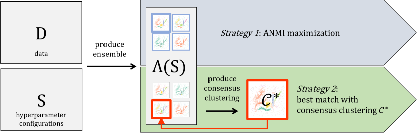
Figure 1: Schema for our proposed method for finding clustering hyperparameters. Here, $\Lambda(S)$ is an ensemble of clusterings of a data set $D$ based on a hyperparameter set $S$ and $\mathcal{C}^{*}$ is the consensus clustering of $\Lambda(S)$. For detailed explanations of the notation, see Section 2.4 and Section 3.

However, one may use outcomes of clustering ensemble aggregation methods such as consensus clustering as formulated by Strehl and Ghosh (2002) as some type of constrained ground truth labeling. In this paper, we propose to apply consensus clustering combined with normalized mutual information (Strehl and Ghosh 2002; Cover and Thomas 2006) as an exemplary external validity measure to classical problems to perform cluster evaluation and compare cluster algorithms and hyperparameters respectively. If the produced clustering ensemble for a specific data set is big and diverse enough, evaluating the individual clusterings relatively to the the aggregated clustering yields information about the quality of each clustering, see Figure 1. Furthermore, as a second strategy for validating individual clusterings, we propose to compare them more directly with the clustering ensemble, in our case using the average normalized mutual information.

This paper is structured as follows: In Section 2, we give a concise overview of normalized mutual information and consensus strategies for clustering problems and introduce our notation. In Section 3, we explain how these techniques can be combined to search for clustering hyperparameters. We present a choice of numerical experiments in Section 4. Concluding with Section 5, we again highlight the general features of our approach and give possible future directions. Appendix A serves as an overview of classically used clustering validation metrics which are employed for comparison in our experiments.

2 Background on NMI and Consensus Clustering

We first introduce our notation and explain the different approaches behind several classical clustering algorithms in Section 2.1. We will illustrate, how the shared information between two clusterings can be measured using the notion of normalized mutual information (NMI) in Section 2.3. Moreover, we explain how multiple clusterings of the same data set can be combined into a so-called consensus clustering, see Section 2.4 and 2.5. This gives the foundation of our proposed methods for finding hyperparameters in Section 3.

2.1 The Clustering Problem

The typical clustering problem setting is as follows: A set $D=\{x_{1},\dots,x_{n}\}\subseteq\mathbb{R}^{d}$ of data points is given. The goal is to define a clustering $\mathcal{C}=\{C_{1},\dots,C_{k}\}$ of $k$ clusters, such that one is either able to map the $x_{i}$ directly onto the clusters $C_{j}$ (hard clustering), or one maps the probability vectors in the $k$-dimensional probability simplex onto the clusters $C_{j}$ (fuzzy clustering). We consider the case of hard clustering in this article, so that $C_{j}\subset D,j=1,\dots,k$. Formally, $\mathcal{C}=\{C_{1},\dots,C_{k}\}$ is a hard clustering of $D$ if

$$C_{i}\cap C_{j}=\emptyset\quad\mbox{and}\quad\bigcup_{i=1}^{k}C_{i}=D.$$

The typical way of expressing a clustering is simply by labeling each data point with the index of its corresponding cluster.

2.2 Cluster comparison criteria

Suppose two clusterings $\mathcal{C}$ and $\mathcal{C}^{\prime}$ are given for the same problem. How should one measure their similarity? In this section, we briefly review some comparison criteria available in the literature.

Since the clusterings are often stored with lists of labels (where each data point is assigned a label or index of some cluster), a common requirement for any such similarity criterion is relabelling invariance, so that two clusterings $\mathcal{C}$ and $\mathcal{C}^{\prime}$ with label lists $(1,1,2,2,2,3)$ and $(3,3,1,1,1,2)$ are considered equal. Viewed differently, permuting the indices of the clusters should not change the similarity measure.

A useful tool is the contingency table or confusion matrix. The confusion matrix for two clusterings $\mathcal{C}=\{C_{1},\ldots C_{K}\}$ and $\mathcal{C}^{\prime}=\{C^{\prime}_{1},\ldots,C^{\prime}_{K^{\prime}}\}$ is a $K\times K^{\prime}$ matrix whose $kk^{\prime}$th entry measures the amount of overlap between clusters $C_{k}$ and $C^{\prime}_{k^{\prime}}$, i.e.

$$n_{kk^{\prime}}=|C_{k}\cup C^{\prime}_{k^{\prime}}|.$$

One category of criteria is based on counting pairs of points. Let $N_{11}$ be the number of pairs of points from $D$ that are in the same cluster under both $\mathcal{C}$ and $\mathcal{C}^{\prime}$, $N_{00}$ the number of pairs of points that are in different clusters under both $\mathcal{C}$ and $\mathcal{C}^{\prime}$, $N_{10}$ the number of point pairs that are in the same cluster under $\mathcal{C}$ but different clusters under $\mathcal{C}^{\prime}$ and $N_{01}$ the number of point pairs that are in different clusters under $\mathcal{C}$ but the same cluster under $\mathcal{C}^{\prime}$. Further, let $n=|D|$. Popular criteria are the Rand index $R(\mathcal{C},\mathcal{C}^{\prime})$ (M. Rand 1971) and Jaccard index $J(\mathcal{C},\mathcal{C}^{\prime})$ (Ben-Hur et al. 2001)

$$R(\mathcal{C},\mathcal{C}^{\prime})=\frac{N_{00}+N_{11}}{n(n-1)/2},\qquad J(\mathcal{C},\mathcal{C}^{\prime})=\frac{N_{11}}{N_{11}+N_{01}+N_{10}}.$$

In order to obtain an index that has range $[0,1]$, the adjusted Rand index $ARI(\mathcal{C},\mathcal{C}^{\prime})$ has been introduced in M. Rand (1971) and Hubert and Arabie (1985)

$$ARI(\mathcal{C},\mathcal{C}^{\prime})=\frac{R(\mathcal{C},\mathcal{C}^{\prime})-\mathbb{E}[R]}{1-\mathbb{E}[R]},$$

where $\mathbb{E}[R]$ is the expectation value of $R$ under a null model. For the detailed definitions of the measures used in our numerical experiments, see Appendix A.

A second category of criteria is based on set matching; each cluster in $\mathcal{C}$ is given a best match in $\mathcal{C}^{\prime}$ and then the total amount of ‘unmatched’ probability mass is computed. See Meilă and Heckerman (2001) and Larsen and Aone (1999) for examples in this category. The common problem of best matching criteria is that they ignore what happens to the unmatched part of the clusterings.

A third category of criteria, which includes the one we use mainly in this paper, is based on information theory. The common idea is to interpret a clustering $\mathcal{C}$ as a discrete valued random variable representing the outcome of drawing a point in $D$ uniformly at random and examining its label. Example criteria include the mutual information discussed below, various normalized variants, and the variation of information considered in Meilă (2007).

2.3 Normalized Mutual Information

For two discrete-valued random variables $X$ and $Y$, whose joint probability distribution is $p_{X,Y}$, the mutual information $I(X,Y)$ is defined as

$$I(X,Y)=\mathbb{E}_{p_{X,Y}}\left[\log\frac{p_{X,Y}}{p_{X}p_{Y}}\right]$$

where $\mathbb{E}_{p}$ denotes the expected value over the distribution $p$. The mutual information measures how much information about $X$ is contained in $Y$ and vice versa. $I(X,Y)$ is not bounded from above. In order to arrive at a comparison criterion with range $[0,1]$, we define the normalized mutual information following (Strehl and Ghosh 2002)

$$NMI(X,Y)=\frac{I(X,Y)}{\sqrt{H(X)H(Y)}}$$ (1)

where

$$H(X)=-\mathbb{E}_{p_{X}}\left[\log p_{X}\right]$$

is the entropy of $X$. The fact that $NMI(X,Y)\in[0,1]$ easily follows from the observation that $I(X,Y)\leq\min(H(X),H(Y))$. Alternative normalizations are possible, e.g. by the joint entropy $H(X,Y)$ Yao (2003), by $\max(H(X),H(Y))$ or by $\frac{1}{2}\ (H(X)+H(Y))$ Kvalseth (1987). We use the normalization (1) in order to be consistent with the framework in Strehl and Ghosh (2002) and because of the similarity to the Pearson correlation coefficient, which normalizes the covariance of two random variables.

The NMI score (1) yields a similarity measure $\phi^{\text{NMI}}(\mathcal{C}_{i},\mathcal{C}_{j})$ for the two clusterings $\mathcal{C}_{i}$ and $\mathcal{C}_{j}$ upon interpreting them as random variables (see Strehl and Ghosh 2002). Let $n_{s}^{i}$ respectively $n_{t}^{j}$ denote the number of $s$-labels in clustering $i$ respectively $t$-labels in clustering $j$. Moreover, let $n_{s,t}$ denote the number of data points, that have label $s$ in clustering $i$ and label $t$ in clustering $j$. Then we define

$$\phi^{\text{NMI}}(\mathcal{C}_{i},\mathcal{C}_{j})=\frac{\sum_{s=1}^{\#\mathcal{C}_{i}}\sum_{t=1}^{\#\mathcal{C}_{j}}n_{s,t}\log\left(\frac{n\cdot n_{s,t}}{n^{i}_{s}\cdot n^{j}_{t}}\right)}{\sqrt{\left(\sum_{s=1}^{\#\mathcal{C}_{i}}n_{s}\log\left(\frac{n_{s}^{i}}{n}\right)\right)\left(\sum_{t=1}^{\#\mathcal{C}_{j}}n_{t}\log\left(\frac{n_{t}^{j}}{n}\right)\right)}},$$

where $\#\mathcal{C}_{i}$, $\#\mathcal{C}_{j}$ denote the number of clusters in the clusterings $\mathcal{C}_{i}$ and $\mathcal{C}_{j}$, respectively. We note that $\phi^{\text{NMI}}(\mathcal{C}_{i},\mathcal{C}_{j})$ is invariant under relabeling, as required above. If either $\mathcal{C}_{i}$ or $\mathcal{C}_{j}$ only contains a single cluster, then the corresponding entropy is zero, and we define $\phi^{\text{NMI}}(\mathcal{C}_{i},\mathcal{C}_{j})$ to be zero as well.

Given an ensemble of $m$ clusterings $\Lambda=\{\mathcal{C}_{1},\ldots,\mathcal{C}_{m}\}$, in order to compare the information that a single clustering $\mathcal{C}$ (not necessarily part of the ensemble) shares with the ensemble $\Lambda$, the averaged normalized mutual information (ANMI) is defined (see Strehl and Ghosh 2002) as

$$\phi^{\text{ANMI}}(\mathcal{C},\Lambda)=\frac{1}{m}\sum_{i=1}^{m}\phi^{\text{NMI}}(\mathcal{C},\mathcal{C}_{i}).$$

For easier notation, we refer to $\phi^{\text{NMI}}$ and $\phi^{\text{ANMI}}$ simply by NMI and ANMI respectively.

2.4 Consensus Clustering

The idea of consensus clustering (also termed ensemble clustering) is to generate a set of $m$ initial clusterings $\Lambda=\{\mathcal{C}_{1},\dots,\mathcal{C}_{m}\}$ of some data set and obtain a final clustering result $\mathcal{C}^{*}$ by integrating the initial results (see Vega-Pons and Ruiz-Shulcloper 2011; Ghosh and Acharya 2011). As the name suggests, $\mathcal{C}^{*}$ should represent a “consensus” or common denominator among all given initial clusterings from the ensemble. Therefore one would want to aim for a consensus clustering $\mathcal{C}^{*}$ with a high ANMI compared to the ensemble of clusterings, that is

$$\mathcal{C}^{*}=\operatorname*{arg\,max}_{\mathcal{C}}\phi^{\text{ANMI}}(\mathcal{C},\Lambda),$$ (2)

where the maximum is taken over a class of conceivable clusterings of the data.

The introduction of the consensus clustering strategy is motivated by two issues that are notorious for existing clustering techniques: (i) Different clustering algorithms make different assumptions about the structure of the data, rendering the right choice of algorithm difficult if that structure is not known, (ii) it is difficult to choose hyperparameters for those algorithms that have them.

Generating a set of initial clusterings $\Lambda$ can be done either by using one classical clustering algorithm with various hyperparameter settings or different initializations, or by clustering the data using different clustering algorithms. It is advisable to use clustering algorithms that work well for the intrinsic structure of the data if it is known beforehand. Otherwise, a variety of clustering algorithms may be used so that the consensus clustering integrates as much information as possible.

2.5 Computation of consensus clusterings

Computing the consensus clustering by direct brute force maximization of (2) is not tractable since the number of possible consensus labellings grows exponentially in the number of data points. On the other hand, greedy algorithms are computationally not feasible and lead to local maxima according to Strehl and Ghosh (2002). Therefore, one needs to find good heuristics and rather use (2) as an evaluation measure. Several approaches for finding the consensus clustering $\mathcal{C}^{*}$ are discussed in the literature (Vega-Pons and Ruiz-Shulcloper 2011; Xu et al. 2012). In this paper, we give two possibilities (Strehl and Ghosh 2002).

Reclustering points.

This approach uses some distance

$$d_{p}:\{x_{1},\dots,x_{n}\}\times\{x_{1},\dots,x_{n}\}\to\mathbb{R}^{+}_{0}$$

on the data points in the following way: For each pair of points $(x_{i},x_{j})$ one can count the number of clusterings from $\Lambda$, in which $x_{i}$ and $x_{j}$ have a different label. That is, $d_{p}$ is the Hamming distance (Hamming 1950) on the points in this case. Then to get $\mathcal{C}^{*}$, one reclusters the points with a similarity based clustering algorithm, i.e. one that only requires a distance metric between the points as input, opposed to coordinates in Euclidean space. Examples include the agglomerative hierarchical clustering method (Ward Jr 1963) and spectral clustering (Ng et al. 2002).

Meta-clustering.

Another possibility is to introduce a distance $d_{C}$ on the set $\{C\in\mathcal{C}_{l}:l=1,\dots m\}$ containing all clusters from the clusterings of the ensemble and to cluster these into “meta-clusters”. Therefore, any data point $x$ is appearing $m$ times in this “meta-clustering” and is finally assigned to the meta-cluster, that it belongs most often to.

Although the second approach should be computationally more efficient than the first approach, one needs to implement a graph partitioning algorithm, if one follows Strehl and Ghosh (2002). The first approach on the other hand is easier to understand and implement, and thus we choose this method for our experiments in Section 4 and employ hierarchical clustering as the similarity based clustering method. Note that the focus of this paper is not the choice of the consensus function, but to present a framework for finding hyperparameters of clustering algorithms.

There is one more subtlety to computing the consensus clustering using this approach: Most consensus clustering methods require the practitioner to know the number of clusters $k^{*}$ for the computation of $\mathcal{C}^{*}$ in advance. Anyhow, our aim is to find clustering algorithm hyperparameters and not exchanging one choice for another. Therefore, we will show in an example, that for large enough $k^{*}$, the hyperparameters determined by our algorithm using consensus clustering is invariant under the choice of $k^{*}$, so that this does not pose a problem. Moreover, there are heuristics to choose $k^{*}$ in a principled way. See Sections 3 and 4.1.1 for more details.

3 Hyperparameter Search using NMI and ANMI

Our proposed approach for finding a reasonable choice of hyperparameters for some given clustering algorithms is twofold: First, an ensemble of clusterings $\Lambda$ is produced by varying the hyperparameters and clustering algorithms considered. Second, the point in parameter space is identified which produced the clustering that shared the most information given by the ensemble $\Lambda$. We will consider two strategies for finding this clustering. For a visual representation of the two approaches, see Figure 1.

For the sake of easier notation, we view the choice of a clustering algorithm as a hyperparameter as well. Having that in mind, let $S$ denote the finite set of all considered hyperparameter configurations, $\mathcal{C}(s)$ the clustering according to the hyperparameter configuration $s\in S$ and let $\Lambda(S)=\{\mathcal{C}(s):s\in S\}$ be the set of all clusterings depending on $S$. The simplest choice for $S$ is a grid search such that $S=P^{(1)}\times\dots\times P^{(l)}$ where $P^{(i)}$ denotes the range of hyperparameter $i$.

Strategy 1: ANMI maximization.

Optimal hyperparameters are selected according to their ANMI (averaged normalized mutual information) score. The “ANMI-best” hyperparameter configuration $s^{\text{ANMI}}$ is thus defined as

$$s^{\text{ANMI}}=\operatorname*{arg\,max}_{s\in S}\phi^{\text{ANMI}}(C(s),\Lambda(S)\setminus\{C(s)\}).$$

Strategy 2: Best match with consensus clustering.

Rather than aggregating information over $\Lambda(S)$ with the ANMI score, we aggregate information over $\Lambda(S)$ by constructing a consensus clustering $\mathcal{C}^{*}$ from $\Lambda(S)$ (as described in Section 2.5). We then select optimal hyperparameters according to their NMI score with $\mathcal{C}^{*}$, that is

$$s^{*}=\operatorname*{arg\,max}_{s\in S}\phi^{\text{NMI}}(\mathcal{C}(s),\mathcal{C}^{*}).$$

This idea translates into the following algorithm 1.

Input: Set $S$ of hyperparameter configurations for chosen clustering algorithms; consensus clustering algorithm with chosen hyperparameters; data $D=\{x_{1},\dots,x_{n}\}$ to cluster

Output: Optimal (in the sense of the NMI-criterion) hyperparameter configuration $s^{*}\in S$

foreach $s\in S$ do

       Produce clustering $\mathcal{C}(s)$ with hyperparameter configuration $s$ and with the corresponding clustering algorithm

end foreach

Produce consensus clustering $\mathcal{C}^{*}$ based on $\Lambda(S)$

return $s^{*}=\operatorname*{arg\,max}_{s\in S}\phi^{\text{NMI}}(\mathcal{C}(s),\mathcal{C}^{*})$

Algorithm 1 Hyperparameter search using Strategy 1

Note that one might also use other normalizations for measuring mutual information or different external clustering similarity measures like the adjusted Rand index $ARI(\mathcal{C},\mathcal{C}^{\prime})$. See Subsection 4.2 for an experimental comparison.

When applying Strategy 2 we need to compute the consensus clustering. Often the hyperparameter $k^{*}$ is needed as an input, i.e. the number of clusters that have to be chosen for computing the consensus clustering. Since we want to find hyperparameters for a clustering method, we have to address the problem of this additional hyperparameter. In 4.1.1 our clustering experiments indicate that Strategy 2 is very robust regarding the choice of $k^{*}$, when $k^{*}$ is at least large enough. Therefore, just choosing a large enough $k^{*}$ should suffice. However, there are even more ways to avoid this restriction, one possible solution is to use the PAC (proportion of ambiguous clustering) measure (Senbabaoğlu et al. 2014; Senbabaoglu et al. 2014; Monti et al. 2003) to infer the optimal $k^{*}$ by minimizing PAC over clusterings from the ensemble with different $k$. This can be performed as a preparation step for Strategy 2.

Computational complexity.

Considering their computational complexity, the two strategies differ. Both algorithms might not be feasible in all situations. Denoting the number of data points with $n$, the typical number of clusters with $k$ and the number of clusterings in the ensemble with $m$, we can do a naïve computational complexity analysis. For computing our consensus function, we computed the Hamming distance for every pair of data points, which is $O(n^{2}m)$. Using agglomerative hierarchical clustering is $O(n^{2}\log(n))$ in general. Moreover, for one NMI-evaluation, we need to go through all data points to count cluster label pairs, which is $O(n)$, and then add $O(k^{2})$ terms in the enumerator, which, for $m$ clusterings in the ensemble, yields $O(mn+mk^{2})$. In total, algorithm 1 costs $O(n^{2}\log(n)+mn+k^{2}m)$. In contrast, finding the ANMI maximizing (Strategy 1) clustering costs one NMI-evaluation for every pair of the $m$ clusterings, i.e. $O(nm^{2})$. In summary, algorithm 1 scales worse in the number of data points, whereas finding the ANMI maximizing (Strategy 1) clustering scales worse in the number of clusterings in the ensemble.

4 Experimental Results

We will give some examples of applying the strategies proposed in the previous section on two synthetic data sets and one real-world data set. Namely we apply the algorithm for finding the best hyperparameter configuration on a very fuzzy data set, see Section 4.1.1 and a data set of handwritten digits in Section 4.2. Moreover we present the results of using the algorithm for finding the best clustering method on a synthetic data set in Section 4.1.2. In each case the resulting clustering of the two strategies can be compared to the consensus clustering. For the algorithmic experiments, we implemented the methods in Python relying heavily on the Scikit-Learn library (Pedregosa et al. 2011).

For testing our proposed methods, we perform the following steps: First, we choose one or several classical clustering algorithms and hyperparameter configurations for each, i.e. we set $S$ in order to generate our set of initial clusterings $\Lambda(S)$ on a grid. Second, we construct the consensus clustering as described in Section 2.5 using the Hamming distance and hierarchical clustering. Next, the NMI of each clustering from $\Lambda(S)$ with the consensus clustering is evaluated. We additionally calculate the ANMI of the consensus clustering as well as of each clustering with the remaining clusterings. The average normalized mutual information of a clustering with a set of clusterings is one heuristic to measure how good they agree, i.e. it measures the shared information between the clustering and set of clusterings. Thus it would be desirable for the consensus clustering to have a high ANMI with $\Lambda(S)$. And last, we find the hyperparameter configuration of the ANMI maximization (Strategy 1) and of the best match with the consensus clustering (Strategy 2) and analyze the results.

4.1 Experiments on synthetic data

We chose two very different artificial data sets. For the “fuzzy” data set we estimate the best DBSCAN hyperparameters in the following. However, for the “spiral” data set we will estimate not only the best hyperparameters but also test which clustering algorithm should be preferred.

4.1.1 Finding hyperparameters for DBSCAN: The fuzzy data set

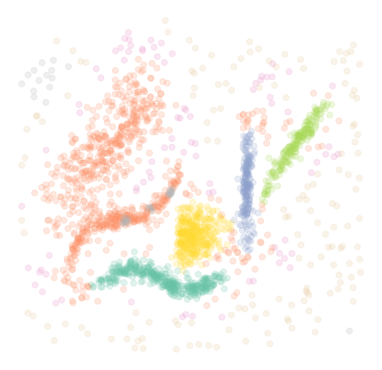
(a) Consensus clustering $\mathcal{C}^{*}$,
ANMI = 0.356

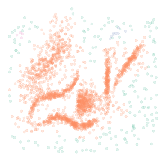
(b) Strategy 1 clustering,
ANMI = 0.372 , NMI = 0.38

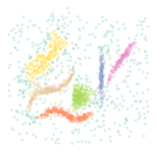
(c) Strategy 2 clustering,
ANMI = 0.292, NMI = 0.813

Figure 2: The “fuzzy” synthetic data set contains fuzzy, non-blob-shaped clusters and many noisy data points. The clusterings chosen by Strategy 1 and Strategy 2 over a grid of clusterings (see Figure 3) are shown here.

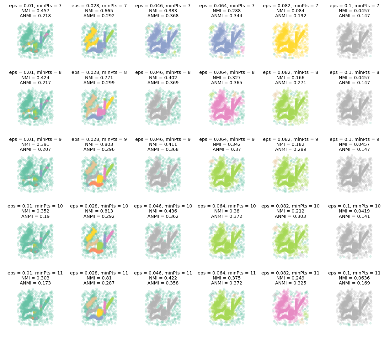
Figure 3: DBSCAN clusterings over a grid of hyperparameters for the “fuzzy” data set. We varied $\varepsilon$ and $m_{\mathrm{points}}$ to produce $\Lambda(S)$ on a grid. In order to generate the consensus clustering, the number of clusters has to be set, here we set $k^{*}=10$. For each clustering we computed the NMI with the consensus clustering (see Figure 2) and the ANMI with the set of clusterings.

The “fuzzy” data set (McInnes 2017) contains some non-globular clusters and some noise and is therefore not easy to cluster for most clustering algorithms. The data set consists of 2309 two-dimensional data points. To generate the set of initial clusterings $\Lambda$ we used the DBSCAN clustering algorithm with a range of different hyperparameters (in particular we varied $\varepsilon$ and $m_{\mathrm{points}}$). Density Based Spatial Clustering of Applications with Noise (DBSCAN) was first proposed by Ester et al. (1996) and is the most commonly used density based clustering approach in metric spaces. Given a density specification consisting of a radius hyperparameter $\varepsilon$ and a minimal point count hyperparameter $m_{\mathrm{points}}$, the algorithm iterates over the data set and searches clusters of density-connected structures, i.e. areas that satisfy a number of at least $m_{\mathrm{points}}$ in a $\varepsilon$-neighborhood of given cluster members and expanding the detected clusters successively. DBSCAN is very sensitive to its hyperparameters, but if they are well chosen, it is capable of detecting highly non-convex, densely connected structures in the data.

Having constructed the grid of clusterings (see Figure 3), it is not surprising that many clusterings are not very reasonable as DBSCAN is very sensitive to its hyperparameters. The consensus clustering should be a common denominator of all the clusterings. Given $\Lambda(S)$, the consensus clustering $\mathcal{C}^{*}$ can be produced and we can find the best match (Strategy 2) hyperparameter configuration and resulting clustering (see Figure 2).

Surprisingly the consensus clustering doesn’t look as good as the clustering with the best match with $\mathcal{C}^{*}$ (Strategy 2): For example in the consensus clustering, two obviously separate clusters are not clearly distinguished. A possible explanation for this effect is the influence of the substantial number of unreasonable clusterings in the ensemble on $\mathcal{C}^{*}$ (see Figure 3). Nevertheless, already minor indications for distinguishing these two clusters in $\mathcal{C}^{*}$ are enough to increase the NMI-score of the “correct” clustering. Note that NMI also accounts for the size of the clusters.

The results of our algorithms depend on the initially constructed ensemble of clusterings. In the given case, many clusterings in the ensemble contain only one or two clusters, i.e. either the whole data set is one cluster or the structure is one cluster, the noise the other cluster. Therefore the ANMI maximizing clustering (Strategy 1) resembles these two observations (see Figure 2).

The experiments in Figure 2 and 3 used the a priori choice of $k^{*}=10$ for the number of clusters in $\mathcal{C}^{*}$. In Figure 4 we repeat the same experiments but vary $k^{*}\in\{3,6,10,15,25,50\}$. We note that both the reported best match (Strategy 2) clustering as well as the chosen hyperparameters found by Strategy 2 are consistent for all $k^{*}\geq 10$. Looking at the NMI-values for the most reasonable four clusterings in the ensemble, even the second best clustering remains the same for large enough $k^{*}$.

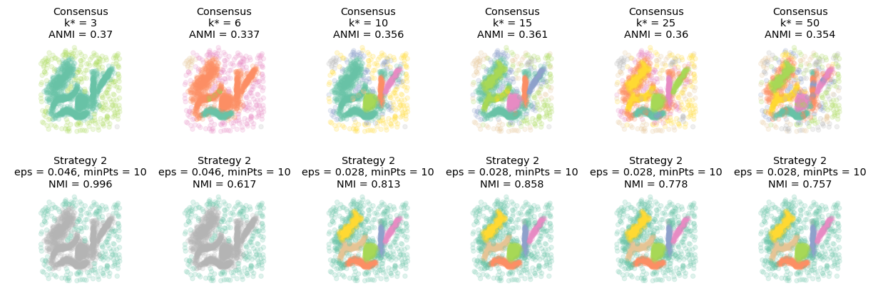
Figure 4: Consensus clusterings and the best match (Strategy 2) clusterings for different values of the number of clusters in the consensus clustering $k^{*}\in\{3,6,10,15,25,50\}$. For each Strategy 2 clustering, the found hyperparameters $s^{*}$ are given. The clustering ensemble is the same DBSCAN ensemble as in Figure 3. If $k^{*}$ is chosen to be large enough, the choice of the clustering always remains the same.

4.1.2 Finding the appropriate algorithm plus hyperparameters: The spiral data set

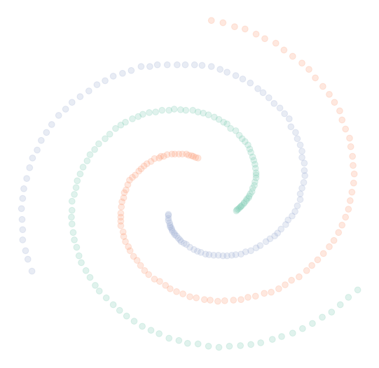
(a) Consensus clustering $\mathcal{C}^{*}$,
ANMI = 0.58

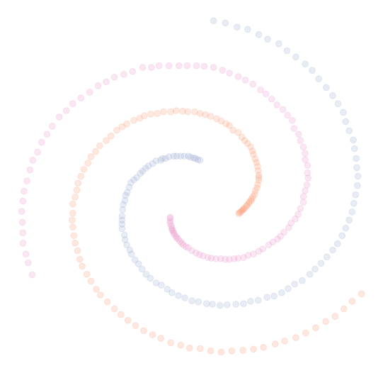
(b) Strategy 1 clustering,
ANMI = 0.58 , NMI = 1.0

(c) Strategy 2 clustering,
ANMI = 0.58 , NMI = 1.0

Figure 5: Synthetic spiral data set embedded in 2D. The data points form three spiral arms corresponding to three clusters. In this example, the results of our algorithms all lead to the same clustering as the consensus clustering, see Figure 6 for the grid of clusterings.

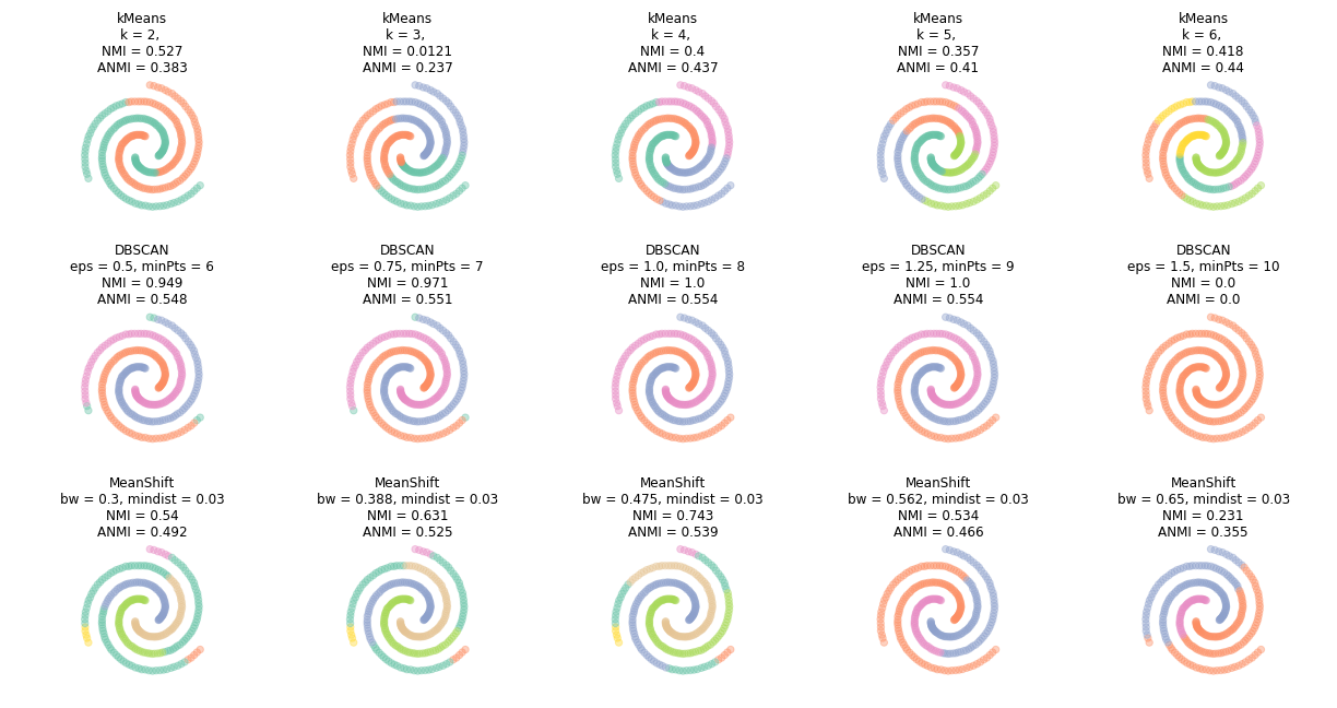
Figure 6: Clusterings over a grid of different algorithms for the spiral data set, namely for (i) k-Means (first row), (ii) DBSCAN (second row) and, (iii) Mean Shift (third row). (i) It is expected that k-Means performs badly, the NMI with $\mathcal{C}^{*}$ is quite low. On the other hand (ii) DBSCAN does very well even for dissimilar hyperparameters. Two clusterings on the grid even share all information with $\mathcal{C}^{*}$. And in the last row (iii), the Mean Shift algorithm outperforms k-Means, but doesn’t produce an outcome as good as DBSCAN. For producing $\mathcal{C}^{*}$ the number of clusters was set to $k^{*}=3$.

The spiral data set (Fränti 2015) contains three spiral arms and no noise or outliers. It consists of 312 data points in $\mathbb{R}^{3}$. The difficulty lies in the fact that the spiral arms, which form the clusters, are elongated and not blob-shaped at all. We chose to use k-Means (see Lloyd 1982; MacQueen et al. 1967), DBSCAN and the Mean Shift algorithm over a range a hyperparameters to generate the set of clusterings $\Lambda(S)$ (see Figure 6). The k-Means algorithm works well on blob-shaped data, thus one wouldn’t expect that it produces reasonable clusterings for any hyperparameter configuration here. Both DBSCAN and Mean Shift are density-based and thus could give good results on the spiral data set. The Mean Shift clustering approach builds on the idea that the data points represent samples from some underlying probability density function. It is an iterative algorithm in which the data points are shifted in the direction of maximum increase in the data sets’ density until convergence (Comaniciu and Meer 2002). Choosing a sensible bandwidth hyperparameter is essential for a good clustering outcome.

To generate $\Lambda(S)$ we varied the number of clusters $k$ for K-Means, for DBSCAN we used different values of $\varepsilon$ and $m_{\mathrm{points}}$ and for the Mean Shift algorithm we varied the bandwidth and minimum distance. The produced grid of clusterings and hyperparameter configurations can be seen in Figure 6. As expected k-means does not produce good clustering results on this type of data, neither does the Mean Shift algorithm for the chosen hyperparameter configurations, but DBSCAN produces very satisfying results.

The consensus clustering combines the clusterings from $\Lambda(S)$ and is able to distinguish the three spiral arms as three clusters, see Figure 5. The two satisfying clustering results generated using DBSCAN have NMI 1.0 with the consensus, i.e. they are exactly the same. Thus the best match (Strategy 2) hyperparameter configurations will give the same result as the consensus clustering. In this example, also the ANMI maximizing (Strategy 1) clustering is the same clustering as the consensus clustering. Our two algorithms thus yield the same clustering result.

4.2 Experiments on real-world data: The digit data set

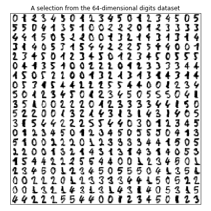
Figure 7: The digits data set (Lichman 2013) consists of preprocessed $8\times 8$ images, thus each data point is 64-dimensional. For visual verification purposes with 2D embeddings, we only used the handwritten digits $0$ to $5$ of which there are $1038$.

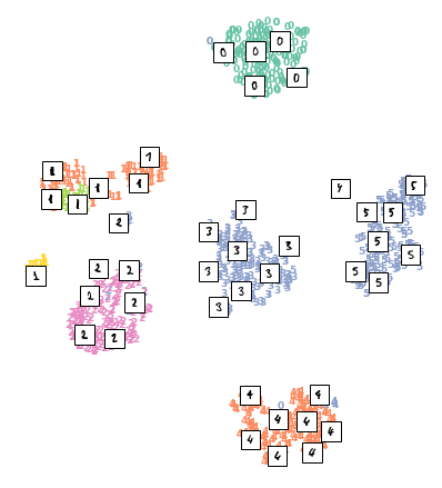
(a) Consensus clustering $\mathcal{C}^{*}$,
ANMI = 0.188

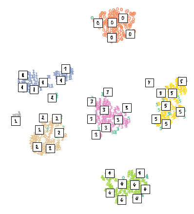
(b) Strategy 1 clustering,
ANMI = 0.193 , NMI = 0.816

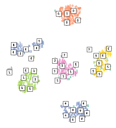
(c) Strategy 2 clustering,
ANMI = 0.188, NMI = 0.834

Figure 8: Results of our methods on a grid of different hyperparameters for DBSCAN. The digits data set is embedded in 2D using the t-distributed Stochastic Neighbor Embedding. For the underlying clustering ensemble, we refer the reader to Figure 9.

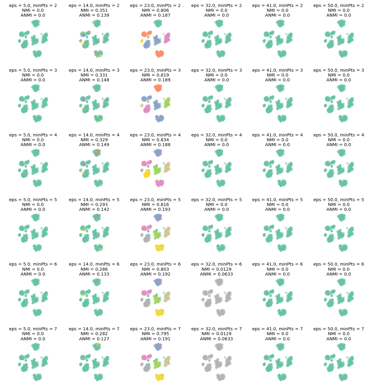
Figure 9: Grid of clusterings for the digits data over a range of DBSCAN hyperparameters. To produce the consensus clustering, the number of clusters was set to $k^{*}=6$. The digits data set is embedded in 2D using the t-distributed Stochastic Neighbor Embedding.

	$\varepsilon=5.0$	$\varepsilon=14.0$	$\varepsilon=23.0$	$\varepsilon=32.0$	$\varepsilon=41.0$	Hyperpar.
ANMI	0.0	0.14	0.19	0.00	0.0
ARI	0.0	0.12	0.67	0.00	0.0
CHI	–∗	4.34	44.99	–	–
DI1 (max.)	–	0.18	0.32	–	–	$m_{\mathrm{points}}=2$
DI2	–	0.34	0.55	–	–
NMI	0.0	0.35	0.81	0.00	0.0
Silhouette	–	-0.30	0.04	–	–
ANMI	0.0	0.15	0.19	0.00	0.0
ARI	0.0	0.10	0.68	0.00	0.0
CHI	–	6.75	66.25	–	–
DI1	–	0.14	0.19	–	–	$m_{\mathrm{points}}=3$
DI2	–	0.41	0.78	–	–
NMI	0.0	0.33	0.82	0.00	0.0
Silhouette	–	-0.33	0.11	–	–
ANMI	0.0	0.15	0.19	0.00	0.0
ARI (max.)	0.0	0.09	0.69	0.00	0.0
CHI	–	10.46	101.43	–	–
DI1	–	0.14	0.23	–	–	$m_{\mathrm{points}}=4$
DI2	–	0.39	0.93	–	–
NMI (max.)	0.0	0.33	0.83	0.00	0.0
Silhouette	–	-0.26	0.17	–	–
ANMI (max.)	0.0	0.14	0.19	0.00	0.0
ARI	0.0	0.07	0.60	0.00	0.0
CHI (max.)	–	10.69	123.87	–	–
DI1	–	0.12	0.20	–	–	$m_{\mathrm{points}}=5$
DI2	–	0.42	0.92	–	–
NMI	0.0	0.29	0.82	0.00	0.0
Silhouette	–	-0.26	0.20	–	–
ANMI	0.0	0.13	0.19	0.06	0.0
ARI	0.0	0.06	0.59	0.00	0.0
CHI	–	12.65	123.35	2.34	–
DI1	–	0.12	0.20	0.21	–	$m_{\mathrm{points}}=6$
DI2	–	0.40	0.92	1.08	–
NMI	0.0	0.29	0.80	0.01	0.0
Silhouette	–	-0.18	0.20	0.06	–
ANMI	0.0	0.13	0.19	0.06	0.0
ARI	0.0	0.05	0.58	0.00	0.0
CHI	–	21.55	122.83	2.34	–
DI1	–	0.12	0.20	0.21	–	$m_{\mathrm{points}}=7$
DI2 (max.)	–	0.94	0.93	1.08	–
NMI	0.0	0.28	0.79	0.01	0.0
Silhouette (max.)	–	-0.12	0.20	0.06	–

Table 1: A selection of commonly used cluster validation metrics on the clusterings depicted in Figure 9 (rounded values). The maximum value for each metric over the range of hyperparameters is highlighted in red. Definitions of the used measures can be found in Appendix A.
^∗value undefined due to single detected cluster

The digit data set (Lichman 2013) contains labeled handwritten digits and consists of preprocessed $8\times 8$ pixel images (see Figure 7 for some samples). For visual verification purposes, we used the t-distributed Stochastic Neighbor Embedding (Maaten and Hinton 2008) to display a clustered subset of the data (labels corresponding to the digits zero to five) in two dimensions. We want to emphasize that the actual clustering was done in the original space of $8\times 8$ pixels, i.e. not in the space obtained by t-SNE.

We used the DBSCAN algorithm (see Figure 9) with a grid of different $\varepsilon$- and $m_{\text{points}}$-parameters, produced the consensus clustering and calculated the NMI and ANMI for every clustering.

The generated consensus as well as the outcomes of Strategy 1 (ANMI maximization) and Strategy 2 (best match clustering) are shown in Figure 8. The consensus clustering fails to separate the digits “3” and “5” in the data (dark blue). Interestingly, the Strategy 2 clustering distinguishes in between the “3” and “5” (dark blue), but fails to separate the “1” and “4”. The ANMI-maximized (Strategy 1) clustering is able to capture the main classes in the data up to small noise, even though the consensus is not classifying everything correctly.

Moreover, we compare the results to a choice of classical internal clustering validation measures, including Dunn index-type measures (DI, see Dunn 1974), the silhouette coefficient (Rousseeuw 1987) and the Caliński-Harabasz index (CHI, Caliński and Harabasz 1974), as well as external measures like the Rand index (ARI, see M. Rand 1971), see Appendix A for detailed definitions. The Rand index is taken with respect to the computed consensus clustering. From the detailed listing of the measure values in Table 1 we conclude that in this example maximizing other classical clustering measures on the ensemble would not always have the same effect as maximizing NMI (Strategy 2) or ANMI (Strategy 1). Both Strategy 1 and 2 result in similar hyperparameter choices that are also chosen by the Caliński-Harabasz index, respectively by the adjusted Rand index. In some situations (e.g. DI1, DI2), it might even be misleading for the user when picking the inappropriate clustering measure.

It is interesting to note that the same intrinsic measures on $\mathcal{C}^{*}$ (see Table 2) can either be better than all the values observed in the ensemble (DI2), mediocre (CHI) or significantly worse (Silhouette). Thus, $\mathcal{C}^{*}$ itself can often be a poor clustering decision. However, Strategies 1 and 2 do lead to competitive clusterings in terms of most of the measures considered here, with Strategy 1 slightly outperforming Strategy 2.

	Consensus $\mathcal{C}^{*}$	Strategy 1	Strategy 2
CHI	113.42	123.87	101.43
DI	0.20	0.20	0.23
DI2	1.01	0.92	0.93
Silhouette	0.13	0.20	0.17

Table 2: Commonly used internal clustering metric values for ANMI- and best match-maximizers (Strategy 1 and 2 respectively) from Table 1 compared to the consensus clustering $\mathcal{C}^{*}$.

5 Conclusion

In this paper, we introduced a technique to validate and compare elements in a clustering ensemble using aggregated common information about clusters in the ensemble. This very general approach can be modified using different consensus strategies and external clustering or classification accuracy measures. We may furthermore interpret this technique as a way of making use of external verification methods even though a priori there is no external clustering we can compare the results to. To do so, we produced external information by constructing an ensemble of clusterings with different hyperparameters and clustering algorithms, such that the clustering ensemble is diverse with respect to the clusterings. And we make use of the information that is contained in the ensemble by evaluating clusterings against it.

Using normalized mutual information and consensus clustering, as well as the average normalized mutual information, we applied the developed heuristic to artificial as well as real-world data sets in order to

• implicitly compare a clustering to all remaining clusterings in the ensemble,

• search for optimal clustering hyperparameters for a given data set,

• determine a reasonable clustering algorithm for a given problem.

We showed that this method is able to filter for clusterings containing the highest degree of information in a noisy ensemble. In our experiments, the clustering produced with the found optimal hyperparameters, was always better or as good as the consensus clustering $\mathcal{C}^{*}$. This might be due to the fact that “correct” structures are in general more likely to be persistent in multiple clusterings, than “wrong” structures. Therefore, the consensus clustering $\mathcal{C}^{*}$ picks up on the correct structures (though it is perturbed by bad clusterings to some extent), which causes good clusterings to have high NMI with $\mathcal{C}^{*}$.

In the DBSCAN examples, our techniques work particularly well, since for too small bandwidth parameters (large clusters), there is few information to share with the ensemble or the consensus. On the other hand, for too high bandwidth parameters, the information contained in one particular clustering is too detailed to appear in multiple clusterings.

Future research may be conducted in directions such as algorithm complexity reduction (e.g. by using different consensus clustering methods) and parallelization, hyperparameter search in terms of random sampling and application of other quality measures alongside NMI or ANMI. Another question to be investigated is the robustness with respect to the number of clusters given to the consensus clustering as a hyperparameter. One idea of choosing this hyperparameter in a more principled manner could consist in using just the framework of this paper: Constructing an ensemble of consensus clusterings and then using a consensus of those as a hyperprior, which may yield a robust and reasonable choice.

Appendix A Clustering quality measures

This appendix serves as an overview of the used comparison measures in Table 1 from Section 4.2. Throughout this appendix we assume a clustering $\mathcal{C}=\{C_{1},\dots C_{k}\}$ on a data set $D$ and an external clustering $\mathcal{C}^{*}=\{\mathcal{C}^{*}_{1},\dots\mathcal{C}^{*}_{k^{*}}\}$. For our experiment, this external partition is given in terms of the associated consensus.

Adjusted Rand index.

The adjusted Rand index (ARI) is an external measure with values in $[-1,1]$ described in M. Rand (1971) and Hubert and Arabie (1985), see also 2.2. Based on the values $s_{ij}=|C_{i}\cap\mathcal{C}^{*}_{j}|$,

$$\textnormal{ }s_{i}=\sum\limits_{j=1}^{k^{*}}s_{ij}\textnormal{ and }s^{*}_{j}=\sum\limits_{i=1}^{k}s_{ij},$$

it is given as

$$\mathrm{ARI}(\mathcal{C},\mathcal{C}^{*})=\frac{\sum_{ij}\binom{s_{ij}}{2}-\big{[}\sum_{i}\binom{s_{i}}{2}\sum_{j}\binom{s^{*}_{j}}{2}\big{]}/\binom{|D|}{2}}{\frac{1}{2}\big{[}\sum_{i}\binom{s_{i}}{2}+\sum_{j}\binom{s^{*}_{j}}{2}\big{]}-\big{[}\sum_{i}\binom{s_{i}}{2}\sum_{j}\binom{s^{*}_{j}}{2}\big{]}/\binom{|D|}{2}}.$$

Larger ARI values indicate partitions with a higher similarity. An ARI value of $1.0$ describes a perfect matching of two clusterings and under consideration of label permutations.

Caliński-Harabasz index.

The Caliński-Harabasz index (CHI, see Caliński and Harabasz 1974) is an internal measure with values in $[0,\infty)$ defined by

$$\mathrm{CHI}(\mathcal{C})=\dfrac{\frac{1}{k-1}\sum\limits_{i=1}^{k}\|\mu_{i}-\mu\|^{2}}{\frac{1}{|D|-k}\sum\limits_{i=1}^{k}\sum\limits_{x\in C_{i}}\|x-\mu_{i}\|^{2}},$$

where $\mu_{i}$ is the barycenter of cluster $C_{i}$ and $\mu$ is the barycenter of the ground set $D$. A higher value indicates a higher ratio of between-cluster-variance and within-cluster-variance, which is interpreted as a better overall clustering.

Dunn-type indices.

The Dunn-type indices (see Dunn 1974) are internal metrics which are usually defined as a ratio of intercluster distances and intracluster diameters. Several different indices can be formulated by this approach. We use the following definitions:

$$\mathrm{DI_{1}}(\mathcal{C}) =\dfrac{\min\limits_{i\neq j}\left\{\inf\limits_{x\in C_{i},y\in C_{j}}\|x-y\|\right\}}{\max\limits_{i}\left\{\max\limits_{x,y\in C_{i}}\|x-y\|\right\}},$$

$$\mathrm{DI_{2}}(\mathcal{C}) =\dfrac{\frac{1}{\binom{k}{2}}\sum\limits_{i\neq j}\inf\limits_{x\in C_{i},y\in C_{j}}\|x-y\|}{\frac{1}{k}\sum\limits_{i=1}^{n}\max\limits_{x,y\in C_{i}}\|x-y\|}$$

A higher Dunn-index is interpreted as indication of a clustering that is able to separate the data better according to (average) distances of observations with respect to their associated clusters.

Silhouette coefficient.

The silhouette coefficient is an internal measure with values in $[-1,1]$. It was first introduced in Rousseeuw (1987) with the form

$$\mathrm{Silhouette}(\mathcal{C})=\dfrac{1}{|D|}\sum\limits_{x\in D}\dfrac{b(x)-a(x)}{\max\{a(x),b(x)\}},$$

where we assume $x\in C$ and set

$$a(x) =\dfrac{1}{|C|}\sum\limits_{y\in C}\|x-y\|_{2}\textnormal{ and}$$

$$b(x) =\min\limits_{A\neq C}\bigg{(}\dfrac{1}{|A|}\sum\limits_{y\in A}\|x-y\|_{2}\bigg{)}.$$

A higher value of the silhouette coefficient indicates a better average matching of all objects in the ground set to their associated cluster. Note that silhouette coefficients can also be computed for subsets of the clustering or single clusters. However, we only use the given version of the coefficient on the whole clustering.

References

- Ben-Hur et al. [2001] Asa Ben-Hur, Andre Elisseeff, and Isabelle Guyon. A stability based method for discovering structure in clustered data. In Biocomputing 2002, pages 6–17. World Scientific, 2001.
- Bergstra and Bengio [2012] James Bergstra and Yoshua Bengio. Random search for hyper-parameter optimization. Journal of Machine Learning Research, 13:281–305, 2012.
- Caliński and Harabasz [1974] T. Caliński and J. Harabasz. A dendrite method for cluster analysis. Communications in Statistics, 3(1):1–27, 1974.
- Comaniciu and Meer [2002] Dorin Comaniciu and Peter Meer. Mean shift: A robust approach toward feature space analysis. IEEE Transactions on pattern analysis and machine intelligence, 24(5):603–619, 2002.
- Cover and Thomas [2006] Thomas M Cover and Joy A Thomas. Elements of information theory 2nd edition. 2006.
- Dunn [1974] J. C. Dunn. Well-separated clusters and optimal fuzzy partitions. Journal of Cybernetics, 4(1):95–104, 1974. doi: 10.1080/01969727408546059.
- Ester et al. [1996] Martin Ester, Hans-Peter Kriegel, Jörg Sander, Xiaowei Xu, et al. A density-based algorithm for discovering clusters in large spatial databases with noise. In Kdd, volume 96, pages 226–231, 1996.
- Fränti [2015] Pasi Fränti. Clustering datasets, 2015. URL http://cs.uef.fi/sipu/datasets/.
- Ghosh and Acharya [2011] Joydeep Ghosh and Ayan Acharya. Cluster ensembles. Wiley Interdisciplinary Reviews: Data Mining and Knowledge Discovery, 1(4):305–315, 2011.
- Hamming [1950] Richard W Hamming. Error detecting and error correcting codes. Bell Labs Technical Journal, 29(2):147–160, 1950.
- Hubert and Arabie [1985] L. Hubert and F. Arabie. Comparing partitions. Journal of Classification, 2:193–218, 1985.
- Kingma and Ba [2014] Diederik P. Kingma and Jimmy Ba. Adam: A method for stochastic optimization. CoRR, abs/1412.6980, 2014. URL http://arxiv.org/abs/1412.6980.
- Kvalseth [1987] Tarald O Kvalseth. Entropy and correlation: Some comments. IEEE Transactions on Systems, Man, and Cybernetics, 17(3):517–519, 1987.
- Larsen and Aone [1999] Bjornar Larsen and Chinatsu Aone. Fast and effective text mining using linear-time document clustering. In Proceedings of the fifth ACM SIGKDD international conference on Knowledge discovery and data mining, pages 16–22. ACM, 1999.
- Lichman [2013] M. Lichman. UCI machine learning repository, 2013. URL http://archive.ics.uci.edu/ml.
- Lloyd [1982] Stuart Lloyd. Least squares quantization in pcm. IEEE transactions on information theory, 28(2):129–137, 1982.
- M. Rand [1971] William M. Rand. Objective criteria for the evaluation of clustering methods. Journal of the American Statistical Association, 66:846–850, 12 1971.
- Maaten and Hinton [2008] Laurens van der Maaten and Geoffrey Hinton. Visualizing data using t-sne. Journal of Machine Learning Research, 9(Nov):2579–2605, 2008.
- MacQueen et al. [1967] James MacQueen et al. Some methods for classification and analysis of multivariate observations. In Proceedings of the fifth Berkeley symposium on mathematical statistics and probability, volume 1, pages 281–297. Oakland, CA, USA., 1967.
- McInnes [2017] Astels McInnes, Healy. Hierarchical density based clustering. Journal of Open Source Software, The Open Journal, 2(11), 2017.
- Meilă and Heckerman [2001] Marina Meilă and David Heckerman. An experimental comparison of model-based clustering methods. Machine learning, 42(1-2):9–29, 2001.
- Meilă [2007] Marina Meilă. Comparing clusterings—an information based distance. Journal of Multivariate Analysis, 98(5):873 – 895, 2007. ISSN 0047-259X. doi: https://doi.org/10.1016/j.jmva.2006.11.013. URL http://www.sciencedirect.com/science/article/pii/S0047259X06002016.
- Monti et al. [2003] Stefano Monti, Pablo Tamayo, Jill Mesirov, and Todd Golub. Consensus clustering: a resampling-based method for class discovery and visualization of gene expression microarray data. Machine learning, 52(1):91–118, 2003.
- Ng et al. [2002] Andrew Y Ng, Michael I Jordan, and Yair Weiss. On spectral clustering: Analysis and an algorithm. In Advances in neural information processing systems, pages 849–856, 2002.
- Pedregosa et al. [2011] F. Pedregosa, G. Varoquaux, A. Gramfort, V. Michel, B. Thirion, O. Grisel, M. Blondel, P. Prettenhofer, R. Weiss, V. Dubourg, J. Vanderplas, A. Passos, D. Cournapeau, M. Brucher, M. Perrot, and E. Duchesnay. Scikit-learn: Machine learning in Python. Journal of Machine Learning Research, 12:2825–2830, 2011.
- Rousseeuw [1987] Peter Rousseeuw. Silhouettes: A graphical aid to the interpretation and validation of cluster analysis. J. Comput. Appl. Math., 20(1):53–65, November 1987. ISSN 0377-0427. doi: 10.1016/0377-0427(87)90125-7. URL http://dx.doi.org/10.1016/0377-0427(87)90125-7.
- Senbabaoglu et al. [2014] Yasin Senbabaoglu, George Michailidis, and Jun Z Li. A reassessment of consensus clustering for class discovery. Sci Rep, 6207, 2014.
- Senbabaoğlu et al. [2014] Yasin Senbabaoğlu, George Michailidis, and Jun Z Li. Critical limitations of consensus clustering in class discovery. Scientific reports, 4, 2014.
- Strehl and Ghosh [2002] Alexander Strehl and Joydeep Ghosh. Cluster ensembles—a knowledge reuse framework for combining multiple partitions. Journal of machine learning research, 3(Dec):583–617, 2002.
- Vega-Pons and Ruiz-Shulcloper [2011] Sandro Vega-Pons and José Ruiz-Shulcloper. A survey of clustering ensemble algorithms. International Journal of Pattern Recognition and Artificial Intelligence, 25(03):337–372, 2011.
- Vinh et al. [2010] Nguyen Xuan Vinh, Julien Epps, and James Bailey. Information theoretic measures for clusterings comparison: Variants, properties, normalization and correction for chance. Journal of Machine Learning Research, 11(Oct):2837–2854, 2010.
- Ward Jr [1963] Joe H Ward Jr. Hierarchical grouping to optimize an objective function. Journal of the American statistical association, 58(301):236–244, 1963.
- Xu et al. [2012] Sen Xu, Tian Zhou, and Hua Long Yu. Analysis and comparisons of clustering consensus functions. In 2nd International Conference on Electronic & Mechanical Engineering and Information Technology. Atlantis Press, 2012.
- Yao [2003] YY Yao. Information-theoretic measures for knowledge discovery and data mining. In Entropy Measures, Maximum Entropy Principle and Emerging Applications, pages 115–136. Springer, 2003.