Copula Variational Bayes inference
via information geometry

Abstract

Variational Bayes (VB), also known as independent mean-field approximation, has become a popular method for Bayesian network inference in recent years. Its application is vast, e.g. in neural network, compressed sensing, clustering, etc. to name just a few. In this paper, the independence constraint in VB will be relaxed to a conditional constraint class, called copula in statistics. Since a joint probability distribution always belongs to a copula class, the novel copula VB (CVB) approximation is a generalized form of VB. Via information geometry, we will see that CVB algorithm iteratively projects the original joint distribution to a copula constraint space until it reaches a local minimum Kullback-Leibler (KL) divergence. By this way, all mean-field approximations, e.g. iterative VB, Expectation-Maximization (EM), Iterated Conditional Mode (ICM) and k-means algorithms, are special cases of CVB approximation.

For a generic Bayesian network, an augmented hierarchy form of CVB will also be designed. While mean-field algorithms can only return a locally optimal approximation for a correlated network, the augmented CVB network, which is an optimally weighted average of a mixture of simpler network structures, can potentially achieve the globally optimal approximation for the first time. Via simulations of Gaussian mixture clustering, the classification’s accuracy of CVB will be shown to be far superior to that of state-of-the-art VB, EM and k-means algorithms.

I Introduction

Originally, the idea of mean-field theory is to approximate an interacting system by a non-interacting system, such that the mean values of system’s nodes are kept unchanged [1]. Variational Bayes (VB) is a redefined method of mean-field theory, in which the joint probability distribution $f_{\boldsymbol{\theta}}$ of a system is approximated by a free-form independent distribution $\widetilde{f}_{\boldsymbol{\theta}}=\prod_{k=1}^{K}\widetilde{f}_{\theta_{k}}$, such that the Kullback-Leibler (KL) divergence $\text{KL}_{\widetilde{f}_{\boldsymbol{\theta}}||f_{\boldsymbol{\theta}}}$ is minimized [2], $\boldsymbol{\theta}\triangleq\{\theta{}_{1},\theta{}_{2},\ldots,\theta_{K}\}$. The term “variational” in VB originates from “calculus of variations” in differential mathematics, which is used to find the derivative of KL divergence over distribution space [3, 4].

The VB approximation is particularly useful for estimating unknown parameters in a complicated system. If the true value of parameters $\boldsymbol{\theta}$ is unknown, we assume they follow a probabilistic model a-priori. We then apply Bayesian inference, also called inverse probability in the past [5, 6], to minimizing the expected loss function between true value $\boldsymbol{\theta}$ and posterior estimate $\widehat{\boldsymbol{\theta}}(\boldsymbol{x})$. In practice, the computational complexity of posterior estimate $\widehat{\boldsymbol{\theta}}(\boldsymbol{x})$ often grows exponentially with arriving data $\boldsymbol{x}$ and, hence, yields the curse of dimensionality [7]. For tractable computation, as shown in this paper, the VB algorithm iteratively projects the originally complex distribution into simpler independent class of each unknown parameter $\theta_{k}$, one by one, until the KL divergence converges to a local minimum. For this reason, the VB algorithm has been used extensively in many fields requiring tractable parameter’s inference, e.g. in neural networks [8], compressed sensing [9], data clustering [10], etc. to name just a few.

Nonetheless, the independent class is too strict in practice, particularly in case of highly correlated model [2]. In order to capture the dependence in a probabilistic model, a popular method in statistics is to consider a copula class. The key idea is to separate the dependence structure, namely copula, of a joint distribution from its marginal distributions. In this way, the copula concept is similar to nonnegative compatibility functions over cliques in factor graphs [11, 12], although the compatibility functions are not probability distributions like copula. Indeed, a copula $c_{\boldsymbol{\theta}}$ is a joint distribution whose marginals are uniform, as originally proposed in [13]. For example, the copula of a bivariate discrete distribution is a bi-stochastic matrix, whose sum of any row or any column is equal to one [14, 15]. More generally, by Sklar’s theorem [13, 16], any joint distribution $f_{\boldsymbol{\theta}}$ can always be written in copula form $f_{\boldsymbol{\theta}}=c_{\boldsymbol{\theta}}\prod_{k=1}^{K}f_{\theta_{k}}$, in which $c_{\boldsymbol{\theta}}$ fully describes the inter-dependence of variables in a joint distribution. For independent class, the copula density $c_{\boldsymbol{\theta}}$ is merely a constant and equal to one everywhere [14].

In this paper, the novel copula VB (CVB) approximation $\widetilde{f}_{\boldsymbol{\theta}}=\widetilde{c}_{\boldsymbol{\theta}}\prod_{k=1}^{K}\widetilde{f}_{\theta_{k}}$ will extend the independent constraint in VB to a copula class of dependent distributions. After fixing the distributional form of $\widetilde{c}_{\boldsymbol{\theta}}$, the CVB iteratively updates the free-form marginals $\widetilde{f}_{\theta_{k}}$ one by one, similarly to traditional VB, until KL divergence $\text{KL}_{\widetilde{f}_{\boldsymbol{\theta}}||f_{\boldsymbol{\theta}}}$ converges to a local minimum. The CVB approximation will become exact if the form of $\widetilde{c}_{\boldsymbol{\theta}}$ is the same as that of original copula $c_{\boldsymbol{\theta}}$. The study of copula form $c_{\boldsymbol{\theta}}$ is still an active field in probability theory and statistics [14], owing to its flexibility to modeling the dependence of any joint distribution $f_{\boldsymbol{\theta}}$. Also, because the mutual information $f_{\boldsymbol{\theta}}$ is equal to entropy of its copula $c_{\boldsymbol{\theta}}$ [17], the copula is currently an interesting topic for information criterions [18, 19].

In information geometry, the KL divergence is a special case of the Bregman divergence, which, in turn, is a generalized concept of distance in Euclidean space [20]. By reinterpreting the KL minimization in VB as the Bregman projection, we will see that CVB, and its special case VB, iteratively projects the original distribution to a fixed copula constraint space until convergence. Then, similar to the fact that the mean is the point of minimum total distance to data, an augmented CVB approximation will also be designed as a distribution of minimum total Bregman divergence to the original distribution in this paper.

Three popular special cases of VB will also be revisited in this paper, namely Expectation-Maximization (EM) [21, 22], Iterated Conditional Mode (ICM) [23, 24] and k-means algorithms [25, 26]. In literature, the well-known EM algorithm was shown to be a special case of VB [1, 2], in which one of VB’s marginal is restricted to a point estimate via Dirac delta function. In this paper, the EM algorithm will be shown that it does not only reach a local minimum KL divergence, but it may also return a local maximum-a-posteriori (MAP) point estimate of the true marginal distribution. This justifies the superiority of EM algorithm to VB in some cases of MAP estimation, since the peaks in VB marginals might not be the same as those of true marginals.

If all VB marginals are restricted to Dirac delta space, the iterative VB algorithm will become ICM algorithm, which returns a locally joint MAP estimate of the original distribution. Also, for standard Normal mixture clustering, the ICM algorithm is equivalent to the well-known k-means algorithm, as shown in this paper. The k-means algorithm is also equivalent to the Lloyd-Max algorithm [25], which has been widely used in quantization context [27].

For illustration, the CVB and its special cases mentioned above will be applied to two canonical models in this paper, namely bivariate Gaussian distribution and Gaussian mixture clustering. By tuning the correlation in these two models, the performance of CVB will be shown to be superior to that of state-of-the-art mean-field methods like VB, EM and k-means algorithm. An augmented CVB form for a generic Bayesian network will also be studied and applied to this Gaussian mixture model.

I-A Related works

Although some generalized forms of VB have been proposed in literature, most of them are merely variants of mean-field approximations and, hence, still confined within independent class. For example, in [28, 29], the so-called Conditionally Variational algorithm is an application of traditional VB to a joint conditional distribution $\widetilde{f}(\boldsymbol{\theta}|\xi)=\prod_{k=1}^{K}\widetilde{f}_{k}(\theta_{k}|\xi)$, given a latent variable $\xi$. Hence, different to CVB above, the approximated marginal $\widetilde{f}_{\xi}$ was not updated in their scheme. In [30], the so-called generalized mean-field algorithm is merely to apply the traditional VB method to the independent class of a set of variables, i.e. each $\theta_{k}$ consists of a set of variables. In [31], the so-called Structured Variational inference is the same as the generalized mean-field, except that the dependent structure inside the set $\theta_{k}$ is also specified. In summary, they are different ways of applying traditional VB, without changing the VB’s updating formula. In contrast, the CVB in this paper involves new tractable formulae and broader copula constraint class.

The closest form to the CVB of this paper is the so-called Copula Variational inference in [32], which fixes the form of approximated distribution $\widetilde{f}_{\boldsymbol{\theta}|\xi}=\widetilde{c}_{\boldsymbol{\theta}|\xi}\prod_{i=1}^{N}\widetilde{f}_{\theta_{i}|\xi}$ and applies gradient decent method upon the latent variable $\xi$ in order to find a local minimum of KL divergence. In contrast, the CVB in this paper is a free-form approximation, i.e. it does not impose any particular form initially, and provides higher-order moment’s estimates than a mere point estimate. Hence, the fixed-form constraint class in their Copula Variational inference is much more restricted than the free-form copula constraint class of CVB in this paper. Also, the iterative computation for CVB will be given in closed form with low complexity, rather than relying point estimates of gradient decent methods.

I-B Contributions and organization

The contributions of this paper are summarized as follows:

• A novel copula VB (CVB) algorithm, which extends the independent constraint class of traditional VB to a copula constraint class, will be given. The convergence of CVB will be proved via three methods: Lagrange multiplier method in calculus of variation, Jensen’s inequality and the Bregman projection in information geometry. The two former methods have been used in literature for proof of convergence of traditional VB, while the third method is new and provides a unified scheme for the former two methods.

• The EM, ICM and k-means algorithms will be shown to be special cases of the traditional VB, i.e. they all locally minimize the KL divergence under a fixed-form independent constraint class.

• An augmented form of CVB, namely hierarchical CVB approximation, with linear computational complexity for a generic Bayesian network will also be provided.

• In simulations, the CVB algorithm for Gaussian mixture clustering will be illustrated. The classification’s performance of CVB will be shown to be far superior to that of VB, EM and k-means algorithms for this model.

The paper is organized as follows: since the Bregman projection in information geometry is insightful and plays central role to VB method, it will be presented first in section II. The definition and property of copula will then be introduced in section III. The novel copula VB (CVB) method and its special cases will be presented in section IV. The computational flow of CVB for a Bayesian network is studied in section V and will be applied to simulations in section VI. The paper is then concluded in section VII.

Note that, for notational simplicity, the notion of probability density function (p.d.f.) for continuous random variable (r.v.) in this paper will be implicitly understood as the probability mass function (p.m.f) in the case of discrete r.v., when the context is clear.

II Information geometry

In this section, we will revisit a geometric interpretation of one of fundamental measures in information theory, namely Kullback-Leibler (KL) divergence, which is also the central part of VB (i.e. mean-field) approximation. For this purpose, the Bregman divergence, which is a generalization of both Euclidean distance and KL divergence, will be defined first. Two important theorems, namely Bregman pythagorean theorem and Bregman variance theorem, will then be presented. These two theorems generalize the concept of Euclidean projection and variance theorem to the probabilistic functional space, respectively. The Bregman divergence is also a key concept in the field of information geometry in literature [33, 20].

II-A Bregman divergence for vector space

For simplicity, in this subsection, we will define Bregman divergence for real vector space first, which helps us visualize the Bregman pythagorean theorem later.

Figure 1: Illustration of Bregman divergence $\mathcal{D}$ for convex function $\phi$. The hyperplane $\mathcal{H}_{\boldsymbol{\beta}}(\boldsymbol{\alpha})\triangleq\phi(\boldsymbol{\beta})+\left\langle\boldsymbol{\alpha}-\boldsymbol{\beta},\nabla\phi(\boldsymbol{\beta})\right\rangle$ is tangent to $\phi$ at point $\boldsymbol{\beta}$. Note that, if $\phi(\boldsymbol{\alpha})$ is equal to the continuous entropy function $H_{\boldsymbol{\alpha}}(\boldsymbol{\alpha})$, the hyperplane $\mathcal{H}_{\boldsymbol{\beta}}(\boldsymbol{\alpha})$ is equal to the cross entropy $H_{\boldsymbol{\beta}}(\boldsymbol{\alpha})$ from $\boldsymbol{\alpha}$ to $\boldsymbol{\beta}$ and $\mathcal{D}(\boldsymbol{\alpha}||\boldsymbol{\beta})=H_{\boldsymbol{\alpha}}(\boldsymbol{\alpha})-H_{\boldsymbol{\beta}}(\boldsymbol{\alpha})$ is equal to Kullback-Leibler (KL) divergence (c.f. section II-A2).

Definition 1.

(Bregman divergence)
Let $\phi:\mathbb{R}^{K}\rightarrow\mathbb{R}$ be a strictly convex and differentiable function. Given two points $\boldsymbol{\alpha},\boldsymbol{\beta}\in\mathbb{R}^{K}$, with $\boldsymbol{\alpha}\triangleq[\alpha{}_{1},\alpha{}_{2},\ldots,\alpha_{K}]^{T}$ and $\boldsymbol{\beta}\triangleq[\beta{}_{1},\beta{}_{2},\ldots,\beta_{K}]^{T}$, the Bregman divergence $\mathcal{D}:\mathbb{R}^{K}\times\mathbb{R}^{K}\rightarrow\mathbb{R}^{+}$, with $\mathbb{R}^{+}\triangleq[0,+\infty)$ , is defined as follows:

$$\mathcal{D}(\boldsymbol{\alpha}||\boldsymbol{\beta}) \triangleq\mathcal{H}_{\boldsymbol{\alpha}}(\boldsymbol{\alpha})-\mathcal{H}_{\boldsymbol{\beta}}(\boldsymbol{\alpha})$$ (1)

$$=\phi(\boldsymbol{\alpha})-\phi(\boldsymbol{\beta})-\left\langle\boldsymbol{\alpha}-\boldsymbol{\beta},\nabla\phi(\boldsymbol{\beta})\right\rangle,$$

where $\nabla$ is gradient operator, $\left\langle\cdot,\cdot\right\rangle$ denotes inner product and $\mathcal{H}_{\boldsymbol{\beta}}(\boldsymbol{\alpha})\triangleq\phi(\boldsymbol{\beta})+\left\langle\boldsymbol{\alpha}-\boldsymbol{\beta},\nabla\phi(\boldsymbol{\beta})\right\rangle$ is hyperplane tangent to $\phi$ at point $\boldsymbol{\beta}$, as illustrated in Fig. 1.

For simplicity, the notations $\mathcal{D}$ and $\mathcal{D}_{\phi}$ are used interchangeably in this paper when the context is clear. Some well-known properties of Bregman divergence (1) are summarized below:

Proposition 2.

(Bregman divergence’s properties)

1. Non-negativity: $\mathcal{D}(\boldsymbol{\alpha}||\boldsymbol{\beta})\geq 0$.

2. Equality:$\mathcal{D}(\boldsymbol{\alpha}||\boldsymbol{\beta})=0\Leftrightarrow\boldsymbol{\alpha}=\boldsymbol{\beta}$.

3. Asymmetry: $\mathcal{D}(\boldsymbol{\alpha}||\boldsymbol{\beta})\neq\mathcal{D}(\boldsymbol{\beta}||\boldsymbol{\alpha})$ in general.

4. Convexity: $\mathcal{D}(\boldsymbol{\alpha}||\boldsymbol{\beta})$ is convex over $\boldsymbol{\alpha}$, but not over $\boldsymbol{\beta}$ in general.

5. Gradient: $\nabla_{\boldsymbol{\alpha}}\mathcal{D}(\boldsymbol{\alpha}||\boldsymbol{\beta})=\nabla\phi(\boldsymbol{\alpha})-\nabla\phi(\boldsymbol{\beta})$ and $\nabla_{\boldsymbol{\beta}}\mathcal{D}(\boldsymbol{\alpha}||\boldsymbol{\beta})=\nabla^{2}\phi(\boldsymbol{\beta})[\boldsymbol{\beta}-\boldsymbol{\alpha}]$.

6. Affine equivalence class: $\mathcal{D}_{\phi}(\boldsymbol{\alpha}||\boldsymbol{\beta})=\mathcal{D}_{\widetilde{\phi}}(\boldsymbol{\alpha}||\boldsymbol{\beta})$ if $\widetilde{\phi}(\boldsymbol{x})=\phi(\boldsymbol{x})+\left\langle\boldsymbol{\gamma},\boldsymbol{x}\right\rangle+c$, e.g. $\widetilde{\phi}(\boldsymbol{x})=\mathcal{D}_{\phi}(\boldsymbol{x}||\boldsymbol{\beta})$.

7. Three-point property:

$$\mathcal{D}(\boldsymbol{\alpha}||\boldsymbol{\beta})+\mathcal{D}(\boldsymbol{\beta}||\boldsymbol{\gamma})-\mathcal{D}(\boldsymbol{\alpha}||\boldsymbol{\gamma}) =\left\langle\boldsymbol{\beta}-\boldsymbol{\alpha},\underset{\nabla_{\boldsymbol{\beta}}\mathcal{D}(\boldsymbol{\beta}||\boldsymbol{\gamma})}{\underbrace{\nabla\phi(\boldsymbol{\beta})-\nabla\phi(\boldsymbol{\gamma})}}\right\rangle$$ (2)

The points $\{\boldsymbol{\alpha},\boldsymbol{\beta},\boldsymbol{\gamma}\}$ in (2) are called Bregman orthogonal at point $\boldsymbol{\beta}$ if $\left\langle\boldsymbol{\beta}-\boldsymbol{\alpha},\nabla\phi(\boldsymbol{\beta})-\nabla\phi(\boldsymbol{\gamma})\right\rangle=0$.

Proof:

All properties 1-7 are direct consequence of Bregman definition (1). The derivation of well-known properties 1-4 and 6-7 can be found in [20, 34] and [35, 36], respectively, for any $\boldsymbol{x},\boldsymbol{\gamma}\in\mathbb{R}^{K}$, $c\in\mathbb{R}$. In property 6, since $\mathcal{D}_{\phi}(\boldsymbol{x}||\boldsymbol{\beta})$ is both convex and affine over $\boldsymbol{x}$, as defined in (1), we can assign $\widetilde{\phi}(\boldsymbol{x})=\mathcal{D}_{\phi}(\boldsymbol{x}||\boldsymbol{\beta})$. In property 7, the $\nabla_{\boldsymbol{\beta}}$ form is a consequence of gradient property. The gradient property, i.e. the property 5, can be derived from definition (1) as follows: $\nabla_{\boldsymbol{\alpha}}\mathcal{D}_{\phi}(\boldsymbol{\alpha}||\boldsymbol{\beta})=\nabla_{\boldsymbol{\alpha}}\phi(\boldsymbol{\alpha})-\nabla_{\boldsymbol{\alpha}}\left\langle\boldsymbol{\alpha}-\boldsymbol{\beta},\nabla\phi(\boldsymbol{\beta})\right\rangle=\nabla_{\boldsymbol{\alpha}}\phi(\boldsymbol{\alpha})-\nabla\phi(\boldsymbol{\beta})$. Similarly, from (1), we have $\nabla_{\boldsymbol{\beta}}\mathcal{D}_{\phi}(\boldsymbol{\alpha}||\boldsymbol{\beta})=-\nabla_{\boldsymbol{\beta}}\phi(\boldsymbol{\beta})-\nabla_{\boldsymbol{\beta}}\left\langle\boldsymbol{\alpha}-\boldsymbol{\beta},\nabla\phi(\boldsymbol{\beta})\right\rangle=-\nabla_{\boldsymbol{\beta}}\phi(\boldsymbol{\beta})-\left(-\nabla\phi(\boldsymbol{\beta})+\nabla^{2}\phi(\boldsymbol{\beta})[\boldsymbol{\alpha}-\boldsymbol{\beta}]\right)=\nabla^{2}\phi(\boldsymbol{\beta})[\boldsymbol{\beta}-\boldsymbol{\alpha}]$, in which $\nabla^{2}$ denotes Hessian matrix operator. ∎

Remark 3.

The gradient property gives us some insight on Bregman divergence. For example, from gradient property, we can see that $\boldsymbol{\alpha}=\boldsymbol{\beta}$ is the stationary and minimum point of $\mathcal{D}(\boldsymbol{\alpha}||\boldsymbol{\beta})$. Also, $\mathcal{D}(\boldsymbol{\alpha}||\boldsymbol{\beta})$ is convex over $\boldsymbol{\alpha}$ but not over $\boldsymbol{\beta}$ since $\phi(\cdot)$ is a convex function, as shown intuitively in the form of $\nabla_{\boldsymbol{\alpha}}\mathcal{D}(\boldsymbol{\alpha}||\boldsymbol{\beta})$ and $\nabla_{\boldsymbol{\beta}}\mathcal{D}(\boldsymbol{\alpha}||\boldsymbol{\beta})$, respectively. The gradient form $\nabla_{\boldsymbol{\beta}}\mathcal{D}(\boldsymbol{\beta}||\boldsymbol{\gamma})$ in (2) represents the changing value of $\mathcal{D}(\boldsymbol{\beta}||\boldsymbol{\gamma})$ over $\boldsymbol{\beta}$ and, hence, explains the three-point property intuitively, as illustrated in Fig. 2.

Let us now consider the most important property of Bregman divergence in this paper, namely Bregman pythagorean inequality, which defines the Bregman projection over a closed convex subset $\mathcal{X}\subset\mathbb{R}^{K}$.

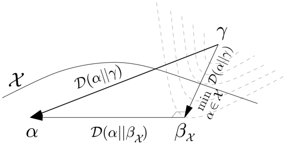
Figure 2: Illustration of Bregman pythagorean inequality over closed convex set $\boldsymbol{\alpha}\in\mathcal{X}$. The point $\boldsymbol{\beta}_{\mathcal{X}}\in\mathcal{X}$ is called the Bregman projection of $\boldsymbol{\gamma}\in\mathbb{R}^{K}$ onto $\mathcal{X}\subset\mathbb{R}^{K}$. The dashed contours represent the convexity of $\mathcal{D}(\boldsymbol{\beta}||\boldsymbol{\gamma})$ over arbitrary point $\boldsymbol{\beta}\in\mathbb{R}^{K}$ in general.

Theorem 4.

(Bregman pythagorean inequality)
Let $\mathcal{X}$ be a closed convex subset in $\mathbb{R}^{K}$. For any points $\boldsymbol{\alpha}\in\mathcal{X}$ and $\boldsymbol{\gamma}\in\mathbb{R}^{K}$, we have:

$$\mathcal{D}(\boldsymbol{\alpha}||\boldsymbol{\beta}_{\mathcal{X}})+\mathcal{D}(\boldsymbol{\beta}_{\mathcal{X}}||\boldsymbol{\gamma})\leq\mathcal{D}(\boldsymbol{\alpha}||\boldsymbol{\gamma}),$$ (3)

where the unique point $\boldsymbol{\beta}_{\mathcal{X}}$ is called the Bayesian projection of $\boldsymbol{\gamma}$ onto $\mathcal{X}$ and defined as follows:

$$\boldsymbol{\beta}_{\mathcal{X}}\triangleq\operatornamewithlimits{arg\,min}_{\boldsymbol{\alpha}\in\mathcal{X}}\mathcal{D}(\boldsymbol{\alpha}||\boldsymbol{\gamma}).$$ (4)

From three-point property (2), we can see that the Bregman pythagorean inequality in (3) becomes equality for all $\boldsymbol{\alpha}\in\mathcal{X}$ if and only if $\mathcal{X}$ is an affine set (i.e. the triple points $\{\boldsymbol{\alpha},\boldsymbol{\beta}_{\mathcal{X}},\boldsymbol{\gamma}\}$ are Bregman orthogonal at $\boldsymbol{\beta}_{\mathcal{X}}$, $\forall\boldsymbol{\alpha}\in\mathcal{X}$).

Proof:

Note that $\boldsymbol{\beta}_{\mathcal{X}}$, as defined in (4), is not necessarily unique if $\mathcal{X}$ is not convex [20]. The uniqueness of $\boldsymbol{\beta}_{\mathcal{X}}$ (4) for convex set $\mathcal{X}$ can be proved either via contradiction [34] or via convexity of $\mathcal{X}$ in three-point property (2), c.f. [20, 37]. Substituting $\boldsymbol{\beta}_{\mathcal{X}}$ in (4) to three-point property (2) yields the Bregman pythagorean inequality (3). ∎

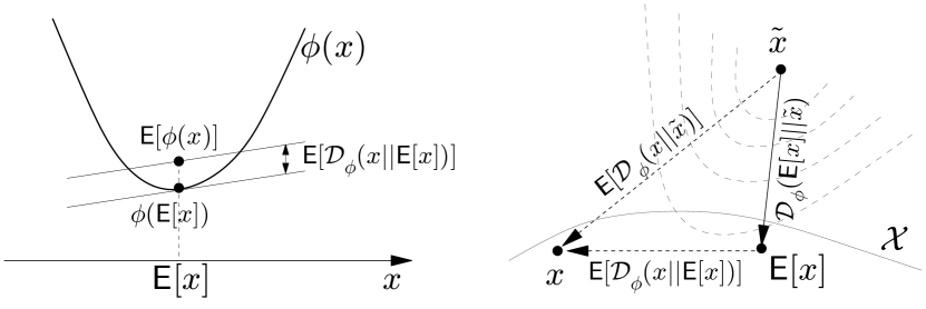
Figure 3: Illustration of equivalence between Jensen’s inequality (left) and Bregman variance theorem (right). Similar to Fig. 1 and Fig. 2, the dashed contours on the right represent the convexity of $\mathcal{D}_{\phi}(\boldsymbol{x}||\widetilde{\boldsymbol{x}})$ over $\boldsymbol{x}$, which, in turn, can be regarded as another convex function $\widetilde{\phi}$ for Jensen’s inequality on the left.

Owing to Bregman divergence, we also have a geometrical interpretation of probabilistic variance, as shown in the following theorem on Jensen’s inequality:

Theorem 5.

(Bregman variance theorem - Jensen’s inequality)
Let $\boldsymbol{x}\in\mathbb{R}^{K}$ be a r.v. with mean $\mathbb{E}[\boldsymbol{x}]$ and variance $\text{Var}[\boldsymbol{x}]$. The Bregman variance $\text{$\text{Var}$}_{\phi}[\boldsymbol{x}]$ is defined as follows:

$$\text{$\text{Var}$}_{\phi}[\boldsymbol{x}]\text{$\triangleq$}\mathbb{E}[\mathcal{D}_{\phi}(\boldsymbol{x}||\mathbb{E}[\boldsymbol{x}])]=\mathbb{E}[\phi(\boldsymbol{x})]-\phi(\mathbb{E}[\boldsymbol{x}])\geq 0.$$ (5)

Equivalently, we have:

$$\text{$\text{Var}$}_{\phi}[\boldsymbol{x}]\text{$\triangleq$}\mathbb{E}[\mathcal{D}_{\phi}(\boldsymbol{x}||\mathbb{E}[\boldsymbol{x}])]=\mathbb{E}[D_{\phi}(\boldsymbol{x}||\widetilde{\boldsymbol{x}})]-\mathcal{D}_{\phi}(\mathbb{E}[\boldsymbol{x}]||\widetilde{\boldsymbol{x}})\geq 0$$ (6)

for any fixed point $\widetilde{\boldsymbol{x}}\in\mathbb{R}^{K}$. The right hand side (r.h.s.) of (5) is called Jensen’s inequality in literature, i.e. $\mathbb{E}(\phi(\boldsymbol{x}))\geq\phi(\mathbb{E}(\boldsymbol{x}))$, for any convex function $\phi$ [38]. Also, from (6), we have:

$$\boldsymbol{x}_{0}\triangleq\mathbb{E}[\boldsymbol{x}]=\operatornamewithlimits{arg\,min}_{\widetilde{\boldsymbol{x}}}\mathbb{E}[D(\boldsymbol{x}||\widetilde{\boldsymbol{x}})],$$ (7)

as illustrated in Fig. 3.

Proof:

Let us show the proof in reverse way. Firstly, the mean property (7) is a consequence of (6), i.e. we have: $\mathbb{E}[D(\boldsymbol{x}||\widetilde{\boldsymbol{x}})]=\mathbb{E}[\mathcal{D}(\boldsymbol{x}||\mathbb{E}[\boldsymbol{x}])]+\mathcal{D}(\mathbb{E}[\boldsymbol{x}]||\widetilde{\boldsymbol{x}})$ and $\mathcal{D}(\mathbb{E}[\boldsymbol{x}]||\widetilde{\boldsymbol{x}})=0\Leftrightarrow\widetilde{\boldsymbol{x}}=\mathbb{E}[\boldsymbol{x}]$. Secondly, by replacing $\phi(\boldsymbol{x})$ in (5) with $\widetilde{\phi}(\boldsymbol{x})=D_{\phi}(\boldsymbol{x}||\widetilde{\boldsymbol{x}})$, the form (6) is equivalent to (5), owing to the affine equivalence property in Proposition 2. Lastly, the form (5) is a direct derivation from Bregman definition (1), with $\boldsymbol{\alpha}=\boldsymbol{x}$ and $\boldsymbol{\beta}=\mathbb{E}[\boldsymbol{x}]$, as follows: $\mathcal{D}(\boldsymbol{x}||\mathbb{E}[\boldsymbol{x}])=\phi(\boldsymbol{x})-\phi(\mathbb{E}[\boldsymbol{x}])-\left\langle\boldsymbol{x}-\mathbb{E}[\boldsymbol{x}],\nabla\phi(\mathbb{E}[\boldsymbol{x}])\right\rangle$ and, hence, $\mathbb{E}[\mathcal{D}(\boldsymbol{x}||\mathbb{E}[\boldsymbol{x}])]=\mathbb{E}[\phi(\boldsymbol{x})]-\mathbb{E}[\phi(\mathbb{E}[\boldsymbol{x}])]-\left\langle\underset{=0}{\underbrace{\mathbb{E}[\boldsymbol{x}]-\mathbb{E}[\boldsymbol{x}]}},\nabla\phi(\mathbb{E}[\boldsymbol{x}])\right\rangle$. ∎

Remark 6.

Although we have $\text{Var}[\boldsymbol{x}]\neq\text{$\text{Var}$}_{\phi}[\boldsymbol{x}]$ in general, the mean $\mathbb{E}[\boldsymbol{x}]$ is the same minimum point for any expected Bregman divergence, as shown in (7). This notable property of the mean has been exploited extensively for Bregman k-means algorithms in literature [34, 35].

A list of Bregman divergences, corresponding to different functional forms of $\phi(\boldsymbol{x})$, can be found feasibly in literature, e.g. in [20, 39]. Let us recall two most popular forms below.

II-A1 Euclidean distance

A special case of Bregman divergence is squared Euclidean distance [35]:

$$\mathcal{D}_{\phi_{E}}(\boldsymbol{\alpha}||\boldsymbol{\beta})=||\boldsymbol{\alpha}-\boldsymbol{\beta}||^{2},\ \text{with}\ \phi_{E}(\boldsymbol{x})\triangleq||\boldsymbol{x}||^{2},$$ (8)

where $||\cdot||$ denotes $\mathcal{L}_{2}$-norm for elements of a vector or matrix. In this case, the Bregman pythagorean theorem (3) becomes the traditional Pythagorean theorem and the Bregman variance (5) becomes the traditional variance theorem, i.e. $\text{$\text{Var}$}_{\phi_{E}}[\boldsymbol{x}]=\text{Var}[\boldsymbol{x}]=\mathbb{E}[||\boldsymbol{x}||^{2}]-||\mathbb{E}[\boldsymbol{x}]||^{2}$.

II-A2 Kullback-Leibler (KL) divergence

Another popular case of Bregman divergence is the KL divergence [35]:

$$\text{KL}(\boldsymbol{\alpha}||\boldsymbol{\beta})\triangleq\mathcal{D}_{\text{KL}}(\boldsymbol{\alpha}||\boldsymbol{\beta})=\sum_{k=1}^{K}\alpha_{k}\log\frac{\alpha_{k}}{\beta_{k}}-\sum_{k=1}^{K}\alpha_{k}+\sum_{k=1}^{K}\beta_{k},$$

with $\phi_{\text{KL}}(\boldsymbol{x})\triangleq\sum_{k=1}^{K}x_{k}\log x_{k}$, $\forall x_{k}\in\mathbb{R}^{+}$. More generally, it can be shown that [39]:

$$\text{KL}{}_{\widetilde{f}||f}\triangleq\mathcal{D}_{\text{KL}}(\widetilde{f}||f)=\mathbb{E}_{\widetilde{f}(\theta)}\log\frac{\widetilde{f}(\theta)}{f(\theta)},$$ (9)

where $\phi_{\text{KL}}(f(\theta))\triangleq H(\theta)=\mathbb{E}_{f(\theta)}\log f(\theta)$ is the continuous entropy and $\mathcal{D}_{\text{KL}}(\widetilde{f}||f)$ is the Bregman divergence between two density distributions $\widetilde{f}(\theta)$ and $f(\theta)$, as presented below.

II-B Bregman divergence for functional space

In the calculus of variations, the Bregman divergence for vector space is a special case of the Bregman divergence for functional space, defined as follows:

Definition 7.

(Bregman divergence for functional space) [33]
Let $\phi:\mathcal{L}_{p}(\theta)\rightarrow\mathbb{R}$ be a strictly convex and twice Fréchet-differentiable functional over $\mathcal{L}_{p}$-normed space. The Bregman divergence $\mathcal{D}:\mathcal{L}_{p}(\theta)\times\mathcal{L}_{p}(\theta)\rightarrow\mathbb{R}^{+}$ between two functions $f,g\in\mathcal{L}_{p}(\theta)$ is defined as follows:

$$\mathcal{D}(f||g) \triangleq\phi(f)-\phi(g)-\delta\phi(f-g;g),$$ (10)

where $\delta\phi(\cdot;g)$ is Fréchet derivative of $\phi$ at $g$.

Apart from gradient form, all well-known properties of Bregman divergence in Proposition 2 are also valid for functional space [33, 40]. Hence, we can feasibly derive the Bregman variance theorem for probabilistic functional space, as follows:

Proposition 8.

(Bregman variance theorem for functions)
Let functional point $f(\theta)$ be a r.v. drawn from the functional space $\mathcal{L}_{p}(\theta)$ with functional mean $\mathbb{E}[f]\triangleq\mathbb{E}[f(\theta)]$ and functional variance $\text{Var}[f]\text{$\triangleq$}\mathbb{E}[||f(\theta)-\mathbb{E}[f]||^{2}]$. Then we have:

$$\text{$\text{Var}$}_{\phi}[f]\text{$\triangleq$}\mathbb{E}\left[\mathcal{D}(f||\mathbb{E}(f))\right]=\mathbb{E}[\phi(f)]-\phi(\mathbb{E}[f])\geq 0.$$

Equivalently, we have:

$$\text{$\text{Var}$}_{\phi}[f]\triangleq\mathbb{E}\left[\mathcal{D}(f||\mathbb{E}(f))\right]=\mathbb{E}[D(f||\widetilde{f})]-\mathcal{D}(\mathbb{E}[f]||\widetilde{f})\geq 0,$$

for any functional point $\widetilde{f}\triangleq\widetilde{f}(\theta)\in\mathcal{L}_{p}(\theta)$ and:

$$f_{0}\triangleq\mathbb{E}[f]=\operatornamewithlimits{arg\,min}_{\widetilde{f}}\mathbb{E}[D(f||\widetilde{f})].$$ (11)

Proof:

Because the Fréchet derivative in (10) is a linear operator like gradient in (1), we can derive the above results in the same manner of the proof of Theorem 5. ∎

Remark 9.

From Proposition 8, we have $\text{Var}[f]=\text{$\text{Var}$}_{\phi_{E}}[f]$ for Euclidean case $\phi_{E}(f)=||f(\theta)-\mathbb{E}[f]||^{2}$, but $\text{Var}[f]\neq\text{$\text{Var}$}_{\phi}[f]$ in general. The functional mean $f_{0}\triangleq\mathbb{E}[f]$ is also the same minimum function for any expected Bregman divergence, similarly to Remark 6.

For later use, let us apply Proposition 8 and show here the Bregman variance for a probabilistic mixture:

Corollary 10.

(Bregman variance theorem for mixture)
Let functional point $f(\theta)$ be a r.v. drawn from a functional set $\boldsymbol{f}\triangleq\{f_{`1}(\theta),\ldots,f_{`N}(\theta)\}$ of $N$ distributions over $\theta$, with probabilities $p_{i}\in\mathbb{I}\triangleq[0,1]$, $\sum_{i=1}^{N}p_{i}=1$. The functional mean (11) is then regarded as a mixture, as follows:

$$f_{0}(\theta)\triangleq\mathbb{E}[f]=\sum_{i=1}^{K}p_{i}f_{i}(\theta),$$ (12)

with variance $\text{Var}[f]\text{=}\sum_{i=1}^{K}p_{i}||f(\theta)-\bar{f}(\theta)||^{2}$. The Bregman variance is then:

$$\text{$\text{Var}$}_{\phi}[f]=\sum_{i=1}^{K}p_{i}D(f_{i}||f_{0})=\sum_{i=1}^{K}p_{i}D(f_{i}||\widetilde{f})-D(f_{0}||\widetilde{f})\geq 0,$$ (13)

for any distribution $\widetilde{f}\triangleq\widetilde{f}(\theta)$ and, hence, from (11-12), we have:

$$f_{0}(\theta)=\mathbb{E}[f]=\sum_{i=1}^{K}p_{i}f_{i}(\theta)=\operatornamewithlimits{arg\,min}_{\widetilde{f}}\sum_{i=1}^{K}p_{i}D(f_{i}||\widetilde{f}).$$ (14)

Proof:

This case is a consequence of Proposition 8. ∎

The case of KL divergence, which is a special case of Bregman variance with $\phi=\phi_{KL}$ in (13), is illustrated in Fig. 4.

Remark 11.

The computation of KL variance via (13) for a mixture is often more feasible than the computation of Euclidean variance in practice. Indeed, the KL form corresponds to geometric mean [39], which can yield linearly computational complexity over exponential coordinates (particularly for exponential family [20, 39]), while the Euclidean form corresponds to arithmetic mean, which would yield exponentially computational complexity for exponential family distributions over Euclidean coordinates in general, as shown in section IV-B3.

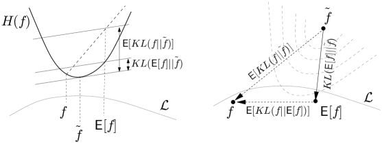
Figure 4: Application of Bregman variance theorem (13) to KL divergence in distribution space $f\in\mathcal{L}$, with the same convention in Fig. 3. As an example, the mixture $f_{0}(\theta)\triangleq\mathbb{E}[f]=\sum_{i=1}^{5}p_{i}f_{i}(\theta)$ in (12) must lie inside the polytope $\mathcal{L}=\{f_{1}(\theta),\ldots,f_{5}(\theta)\}$. In middle sub-figure, $H(f)$ denotes the continuous entropy over p.d.f. $f$. The mixture $\widetilde{f}=f_{0}=\mathbb{E}[f]$ is then the minimum functional point of $\mathbb{E}[\text{KL}(f||\widetilde{f})]$, which is also an upper bound of $\text{KL}(\mathbb{E}[f]||\widetilde{f})$ over $\widetilde{f}\in\mathcal{L}$, as shown in (13-14).

III Copula theory

The copula concept was firstly defined in [13], although it was also defined under different names such as “uniform representation” or “dependence function” [14]. The copula has been studied intensively in many decades in statistics, particularly for finances [41, 42]. Yet the application of copula in information theory is still limited at the moment. In this section, we will review the basic concept of copula and its direct connection to mutual information of a system. The KL divergence for copula, which is the nutshell of CVB approximation in next section, will be provided at the end of this section.

III-A Sklar’s theorem

Because the Sklar’s paper [13] is the beginning of copula’s history, let us recall the Sklar’s theorem first.

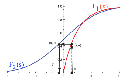
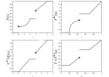
Figure 5: Illustration of variable transformation from $x$ to $s$ in the case of continuous c.d.f. [43] (left), together with pseudo-inverse $F^{\leftarrow}(u)$ of a non-continuous c.d.f. $F(x)$ and their concatenations $F^{\leftarrow}\circ F(x)$, $F\circ F^{\leftarrow}(u)$ [42] (right). We can see that the uniqueness of copula requires the continuous property of c.d.f., since non-continuous c.d.f. does not preserve the inverse transformation.

Definition 12.

(Pseudo-inverse function)
Let $F:\mathbb{R}\rightarrow\mathbb{I}$ be a cumulative distributional function (c.d.f.) of a r.v. $\theta\in\mathbb{R}$. Since $F(\theta)$ is not strictly increasing in general, as illustrated in Fig. 5, a pseudo-inverse function (also called quantile function) $F^{\leftarrow}:\mathbb{I}\rightarrow\mathbb{R}$ is defined as follows:

$$F^{\leftarrow}(u)\triangleq\inf\{\theta\in\mathbb{R}:F(\theta)\geq u\},\ u\in\mathbb{I}.$$

Note that, the quasi-inverse $F^{\leftarrow}$ coincides with the inverse function $F^{-1}$ if $F(\theta)$ is continuous and strictly increasing, as illustrated in Fig. 5.

Theorem 13.

(Sklar’s theorem) [13, 16]
For any r.v. $\boldsymbol{\theta}=[\theta{}_{1},\theta{}_{2},\ldots,\theta_{K}]^{T}\in\mathbb{R}^{K}$ with joint c.d.f. $F(\boldsymbol{\theta})$ and marginal c.d.f. $F_{k}(\theta_{k})$, $\forall k\in\{1,2,\ldots,K\}$, there always exists an equivalent joint c.d.f., namely copula $C$, whose all marginal c.d.f. $C_{k}(F_{k}(\theta_{k}))$ are uniform over $\mathbb{I}$ as follows:

$$F(\boldsymbol{\theta})=C(F_{1}(\theta_{1}),\ldots,F_{K}(\theta_{K}))$$ (15)

In general, the copula form $C$ of a joint c.d.f. $F$ is not unique, but its value on the range $\boldsymbol{u}\in\text{Range}\{F_{1}\}\times\ldots\times\text{Range}\{F_{K}\}\subseteq\mathbb{I}^{K}$ is always unique, as follows:

$$C(\boldsymbol{u})=F(F^{\leftarrow}_{1}(u_{1}),\ldots,F^{\leftarrow}_{K}(u_{K}))$$ (16)

with $\boldsymbol{u}\triangleq[u{}_{1},u{}_{2},\ldots,u_{K}]^{T}$and $u_{k}\triangleq F_{k}(\theta_{k}):\mathbb{R}\rightarrow\mathbb{I}$, $\forall k$. If all marginals $F_{1},\ldots F_{K}$ are continuous, the copula $C$ in (15) is uniquely determined by quantile transformation (16), in which $F^{\leftarrow}$ coincides with the inverse function $F^{-1}$.

III-A1 Bound of copula

For rough visualization of copula, let us recall the Fréchet-Hoeffding bound of copula [14, 42]:

$$\max\{0,1-K+\sum_{k=1}^{K}u_{k})\}\leq C(u_{1},\ldots,u_{K})\leq\min\{u_{1},\ldots,u_{K}\}$$

where $u_{k}\triangleq F_{k}(\theta_{k}):\mathbb{R}\rightarrow\mathbb{I}$. This bound is illustrated in Fig. 6 for the case of two dimensions.

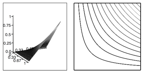
Figure 6: All bivariate copulas must lie inside the pyramid of Fréchet-Hoeffding bound. Both marginal c.d.f. $C(u_{1},1)$ and $C(1,u_{2})$ must be uniform over $[0,1]$ by definition and, hence, plotted in the left sub-figure as straight lines. The two sub-figures on the right illustrates the contours of independent copula $C(u_{1},u_{2})=u_{1}u_{2}$ [41].

III-A2 Discrete copula

The pseudo-inverse form (16) is often called sub-copula in literature [14], since its values are only defined on a possibly subset of $\mathbb{I}^{K}$. This mostly happens in the case of discrete distributions, where marginal $F(\boldsymbol{\theta})$ is not continuous, as illustrated in Fig. 5. Hence, there are possibly more than one continuous copula (15) satisfying the discrete sub-copula form (15) at specific values $\boldsymbol{u}\in\text{Range}\{F_{1}\}\times\ldots\times\text{Range}\{F_{K}\}$.

As illustrated in Fig. 5, the Sklar’s theorem only guarantees the uniqueness of copula form $C$ for a strictly increasing continuous $F$ (c.f. [14] for examples of non-unique copulas $C$ associated with a discrete $F$). Nonetheless, the quantile function in (16) is still useful to compute copula values in the discrete range of $F$. For example, in [14, 15], the copula form of any discrete bivariate distribution was shown to be equivalent to a bi-stochastic non-negative matrix, whose sum of any row or column is equal to one.

III-A3 Continuous copula

For simplicity, let us focus on copula form of continuous c.d.f. $F$, although the results in this paper can be extended to discrete case via pseudo-inverse function in (16). For continuous case, the quantile transformation (16) yields the density form of copula $C$, as follows:

Corollary 14.

(Copula density function) [14]
If all marginals $F_{1},\ldots F_{K}$ are absolutely continuous with respect to Lebesgue measure on $\mathbb{R}^{K}$, the density $c(\boldsymbol{u})\triangleq\frac{\partial C(\boldsymbol{u})}{\partial u_{1}\ldots\partial u_{K}}$ of copula $C$ in (15) is given by:

$$f(\boldsymbol{\theta})=c(\boldsymbol{u}(\boldsymbol{\theta}))\prod_{k=1}^{K}f_{k}(\theta_{k})$$ (17)

where $f$ is density of c.d.f. $F$ and $\boldsymbol{u}\triangleq\boldsymbol{u}(\boldsymbol{\theta})\in\mathbb{I}^{K}$, with $u_{k}\triangleq F_{k}(\theta_{k})$, $\forall k\in\{1,2,\ldots,K\}$.

Proof:

By chain rule, we have $f(\boldsymbol{\theta})=\frac{\partial F(\boldsymbol{\theta})}{\partial\theta_{1}\ldots\partial\theta_{K}}=\frac{\partial C(\boldsymbol{u})}{\partial u_{1}\ldots\partial u_{K}}\prod_{k=1}^{K}\frac{\partial u_{k}}{\partial\theta_{k}}=c(\boldsymbol{u})\prod_{k=1}^{K}f_{k}(\theta_{k})$. ∎

The density (17) shows that a joint p.d.f. can be factorized into two parts: the dependent part represented by copula and the independent part represented by product of its marginals. Hence, the copula fully extracts all dependent relationships between r.v. $\theta_{k}$, $k\in\{1,2,\ldots,K\}$, from joint p.d.f. $f(\boldsymbol{\theta})$.

Remark 15.

Note that, since copula $C$ is essentially a c.d.f. by definition (15), the copula $C(\boldsymbol{u})$ of independent c.d.f. $F(\boldsymbol{\theta})=\prod_{k=1}^{K}F_{k}(\theta_{k})$ is also factorable, i.e. $C(\boldsymbol{u})=\prod_{k=1}^{K}u_{k}$, and, hence, $c(\boldsymbol{u})=1$ by (17), as illustrated in Fig. 6.

III-B Copula’s invariant transformations

Let us focus on continuous copula and its useful transformation’s properties in this subsection. These properties are also satisfied with discrete copulas via pseudo-inverse function (16).

III-B1 Copula’s rescaling transformation

By copula’s density definition (17), we can see that a copula $c(\boldsymbol{u}(\boldsymbol{\theta}))$ is merely a rescaled coordinate form of original joint p.d.f. $f(\boldsymbol{\theta})$, as follows:

Corollary 16.

(Copula’s rescaling property)

$$1=\int_{\boldsymbol{u}(\boldsymbol{\theta})\in\mathbb{I}^{K}}c(\boldsymbol{u})d\boldsymbol{u}=\int_{\boldsymbol{\theta}\in\mathbb{R}^{K}}f(\boldsymbol{\theta})d\boldsymbol{\theta}$$ (18)

Proof:

By definition in (17), we have $u_{k}\triangleq F_{k}(\theta_{k})$ and $d\boldsymbol{\theta}\triangleq\prod_{k=1}^{K}d\theta_{k}$, which yields: $d\boldsymbol{u}=\prod_{k=1}^{K}du_{k}=\prod_{k=1}^{K}f_{k}(\theta_{k})d\boldsymbol{\theta}=\frac{f(\boldsymbol{\theta})}{c(\boldsymbol{u}(\boldsymbol{\theta}))}d\boldsymbol{\theta}.$ Q.E.D. ∎

The rescaling property (18) will be useful later when we wish to change the integrated variables from $\boldsymbol{\theta}$ to $\boldsymbol{u}$ in copula’s manipulation.

III-B2 Copula’s monotone transformation

Under generally monotonic transformation, which is not necessarily strictly increasing, the copula is linearly invariant (c.f. [14] for details). In this paper, let us recall here the useful rank-invariant property of copula under increasing transformation, as follows:

Theorem 17.

(Copula’s rank-invariant property) [42, 14]
Let $\widetilde{\boldsymbol{\theta}}\triangleq[\widetilde{\theta}{}_{1},\widetilde{\theta}{}_{2},\ldots,\widetilde{\theta}_{K}]^{T}\in\mathbb{R}^{K}$, in which $\widetilde{\theta}_{k}\triangleq\varphi_{k}(\theta_{k})$ is a strictly increasing function of r.v. $\theta_{k}\in\mathbb{R}$, $\forall k\in\{1,2,\ldots,K\}$. Then the density copulas $\widetilde{c}$ and $c$ of $\widetilde{\boldsymbol{\theta}}$ and $\boldsymbol{\theta}$, respectively, have the same form, i.e. $\widetilde{c}(\boldsymbol{u})=c(\boldsymbol{u})$, $\forall\boldsymbol{u}\in\mathbb{I}^{K}$.

Intuitively, the copula’s rank-invariant property is merely a consequence of natural rank-invariant property of marginal c.d.f. under increasing transformation, as implied by definition of copula (15) and illustrated in Fig. 5.

III-B3 Copula’s marginal transformation

For later use, let us emphasize a very special case of rank-invariant property, namely marginal transformation. By definition (17), we can see that copula separates the dependence part of joint p.d.f. from its marginals. Hence, we can freely replace any marginal $F_{k}$ with new marginal $\widetilde{F}_{k}$, $\forall k\in\{1,2,\ldots,K\}$, without changing the form of copula, as shown below:

Corollary 18.

(Copula’s marginal-invariant property)
Let $\widetilde{\boldsymbol{\theta}}(\boldsymbol{\theta})\triangleq[\theta_{1},\ldots,\widetilde{\theta}_{k}(\theta_{k}),\ldots,\theta_{K}]^{T}\in\mathbb{R}^{K}$, in which r.v. $\theta_{k}$ in $\boldsymbol{\theta}$ is replaced by a continuously transformed r.v. $\widetilde{\theta}_{k}(\theta_{k})\triangleq\widetilde{F}^{\leftarrow}_{k}(F_{k}(\theta_{k}))$ , for any $k\in\{1,2,\ldots,K\}$. Then the density copulas $\widetilde{c}_{k}$ and $c$ of $\widetilde{\boldsymbol{\theta}}(\boldsymbol{\theta})$ and $\boldsymbol{\theta}$, respectively, have the same form, i.e. $\widetilde{c}_{k}(\boldsymbol{u})=c(\boldsymbol{u})$, $\forall\boldsymbol{u}\in\mathbb{I}^{K}$.

Proof:

This corollary is a direct consequence of the copula’s rank-invariant property, since the continuous c.d.f. functions $\widetilde{F}^{\leftarrow}_{k}$ and $F_{k}$ are both strictly increasing function for continuous variables. ∎

The marginal-invariant property shows that when we replace the marginal distribution $f_{k}(\theta_{k})$ of joint p.d.f. $f(\boldsymbol{\theta})$ in (17) by another marginal distribution $\widetilde{f}_{k}(\theta_{k})$, the resulted joint distribution $\widetilde{f}(\boldsymbol{\theta})$ does not change its original copula form, i.e.:

$$\left.\begin{array}[]{cc}f(\boldsymbol{\theta})&=f(\theta_{\backslash k}|\theta_{k})f_{k}(\theta_{k})\\ \widetilde{f}(\boldsymbol{\theta})&=f(\theta_{\backslash k}|\theta_{k})\widetilde{f}_{k}(\theta_{k})\end{array}\right\}\Rightarrow\widetilde{c}(\boldsymbol{u})=c(\boldsymbol{u}),\forall\boldsymbol{u}\in\mathbb{I}^{K}$$ (19)

Indeed, by Corollary 18, we have $f(\boldsymbol{\theta})=\widetilde{f}(\widetilde{\boldsymbol{\theta}}(\boldsymbol{\theta}))$, i.e. the distribution $\widetilde{f}(\boldsymbol{\theta})$ is merely a marginally rescaling form of $f(\boldsymbol{\theta})$ and, hence, does not change the form of copula.

III-C Copula’s divergence

Because the copula is essentially a distribution itself, the KL divergence (9) can be applied directly to any two copulas. Let us show the relationship between joint p.d.f. and its copula via KL divergence in this subsection.

III-C1 Mutual information

Because all dependencies in a joint p.d.f. $f$ in (17) is captured by its copula, it is natural that the mutual information of joint p.d.f. $f$ can also be computed via its copula form $c$ in (17), as shown below.

Proposition 19.

(Mutual information)
For continuous copula $c$ in (17), the mutual information $I(\boldsymbol{\theta})$ of joint p.d.f. $f(\boldsymbol{\theta})$ is equal to continuous entropy $H$ of copula density $c(\boldsymbol{u}(\boldsymbol{\theta}))$, as follows:

$$I(\boldsymbol{\theta})=H(c(\boldsymbol{u})).$$ (20)

Proof:

The proof is straight-forward from definition of KL divergence (9) and copula density (17), as follows: $I(\boldsymbol{\theta})\triangleq\text{$\text{KL}$}(f(\boldsymbol{\theta})||\prod_{k=1}^{K}f_{k}(\theta_{k}))=\mathbb{E}_{f(\boldsymbol{\theta})}\log\frac{f(\boldsymbol{\theta})}{\prod_{k=1}^{K}f_{k}(\theta_{k})}=\mathbb{E}_{f(\boldsymbol{\theta})}\log c(\boldsymbol{u}(\boldsymbol{\theta}))=\mathbb{E}_{c(\boldsymbol{u})}\log c(\boldsymbol{u})=\text{H}(c(\boldsymbol{u}))$, in which $\boldsymbol{\theta}$ was transformed to $\boldsymbol{u}$ via rescaling property (18). For a special case of bivariate copula density, another proof was given in [17]. ∎

III-C2 KL divergence (KLD)

In literature, the below copula-based KL divergence for a joint p.d.f. was already given for a special case of conditional structure [44]. For later use, let us recall their proof here in a slightly more generally form, via pseudo-inverse (16) and rescaling property (18).

Proposition 20.

(Copula’s divergence) [44]
The KLD of two joint p.d.f. $f$, $\widetilde{f}$ in (17) is the sum of KLD of their copulas $c$, $\widetilde{c}$ and KLDs of their marginals $f_{k}$, $\widetilde{f}_{k}$, as follows:

$$\text{$\text{KL}$}_{\widetilde{f}||f}=\text{$\text{KL}$}(\widetilde{c}(\boldsymbol{u})||c(F(\widetilde{F}^{\leftarrow}(\boldsymbol{u}))))+\sum_{k=1}^{K}\text{$\text{KL}$}_{\widetilde{f}_{k}||f_{k}}$$ (21)

in which the copula $\widetilde{c}$ of $\widetilde{f}$ was rescaled back to marginal coordinates of $f$, i.e. $\widetilde{c}(\widetilde{F}(F^{\leftarrow}(\boldsymbol{u})))\triangleq\widetilde{c}(\widetilde{F}_{1}(F^{\leftarrow}_{1}(u_{1})),\ldots,\widetilde{F}_{K}(F^{\leftarrow}_{K}(u_{K}))).$

Proof:

By definition of KLD (9) and copula density (17), we have: $\text{$\text{KL}$}(f(\boldsymbol{\theta})||\widetilde{f}(\boldsymbol{\theta}))=\mathbb{E}_{f(\boldsymbol{\theta})}\log\frac{f(\boldsymbol{\theta})}{\widetilde{f}(\boldsymbol{\theta})}=\mathbb{E}_{f(\boldsymbol{\theta})}\log\frac{c(\boldsymbol{u}(\boldsymbol{\theta}))}{\widetilde{c}(\tilde{\boldsymbol{u}}(\boldsymbol{\theta}))}+\sum_{k=1}^{K}\mathbb{E}_{f(\boldsymbol{\theta})}\log\frac{f_{k}(\theta_{k})}{\widetilde{f}_{k}(\theta_{k})}$, of which the second term in r.h.s. is actually KLDs of marginal, i.e. $\mathbb{E}_{f(\boldsymbol{\theta})}\log\frac{f_{k}(\theta_{k})}{\widetilde{f}_{k}(\theta_{k})}=\mathbb{E}_{f_{k}(\theta_{k})}\log\frac{f_{k}(\theta_{k})}{\widetilde{f}_{k}(\theta_{k})}=\text{$\text{KL}$}(f_{k}(\theta_{k}))||\widetilde{f}_{k}(\theta_{k}))$ and the first term in r.h.s. is actually KLD of copulas, via rescaling property (18), as follows: $\mathbb{E}_{f(\boldsymbol{\theta})}\log\frac{c(\boldsymbol{u}(\boldsymbol{\theta}))}{\widetilde{c}(\tilde{\boldsymbol{u}}(\boldsymbol{\theta}))}=\mathbb{E}_{f(\boldsymbol{\theta})}\log\frac{c(F_{1}(\theta_{1}),\ldots,F_{K}(\theta_{K}))}{\widetilde{c}(\widetilde{F}_{1}(\theta_{1}),\ldots,\widetilde{F}_{K}(\theta_{K}))}=\mathbb{E}_{c(\boldsymbol{u})}\log\frac{c(\boldsymbol{u})}{\widetilde{c}(\widetilde{F}(F^{\leftarrow}(\boldsymbol{u})))}=\text{$\text{KL}$}(c(\boldsymbol{u})||\widetilde{c}(\widetilde{F}(F^{\leftarrow}(\boldsymbol{u}))))$. ∎

Note that, by copula’s marginal- and rank-invariant properties in section III-B, we can see that the marginal rescaling form $\widetilde{c}(\widetilde{F}(F^{\leftarrow}(\boldsymbol{u})))$ of $\widetilde{c}$ in (21) does not change the original form of copula $\widetilde{c}$.

Remark 21.

If all $\widetilde{F}_{k}$ are exact marginals of $F(\boldsymbol{\theta})$, i.e. $\widetilde{F}_{k}=F_{k}$ in (21), $\forall k\in\{1,2,\ldots,K\}$, we have $\text{$\text{KL}$}(f(\boldsymbol{\theta})||\widetilde{f}(\boldsymbol{\theta}))=\text{$\text{KL}$}(c(\boldsymbol{u})||\widetilde{c}(\boldsymbol{u}))$. Furthermore, if $\widetilde{c}(\boldsymbol{u})$ is also an independent copula, as noted in Remark 15, the KL divergence in (21) will be equal to mutual information $I(\boldsymbol{\theta})$ in (20).

IV Copula Variational Bayes approximation

As shown in (21), the KL divergence between any two distributions can always be factorized as the sum of KL divergence of their copulas and KL divergences of their marginals. Exploiting this property, we will design a novel iterative copula VB (CVB) algorithm in this section, such that the CVB distribution is closest to the true distribution in terms of KL divergence, under constraint of initially approximated copula’s form. The mean-field approximations, which are special cases of CVB, will also be revisited later in this section.

IV-A Motivation of marginal approximation

Let us now consider a joint p.d.f. $f(\boldsymbol{\theta})$, of which the true marginals $f_{k}(\theta_{k})=\int_{\theta_{\backslash k}}f(\boldsymbol{\theta})d\theta_{\backslash k}$, $k\in\{1,2,\ldots,K\},$ are either unknown or too complicated to compute. A natural approximation of $f_{k}(\theta_{k})$ is then to seek a closed form distribution $\widetilde{f}_{k}(\theta_{k})$ such that their KL divergences $\sum_{k=1}^{K}\text{$\text{KL}$}_{f_{k}||\widetilde{f}_{k}}$ in (21) is minimized. This direct approach is, however, not feasible if the integration for true marginal $f_{k}(\theta_{k})$ is very hard to compute at the beginning.

A popular approach in literature is to find an approximation $\widetilde{f}(\boldsymbol{\theta})$ of the joint distribution $f(\boldsymbol{\theta})$ such that their KL divergence $\text{KL}{}_{\widetilde{f}||f}\triangleq\text{KL}(\widetilde{f}(\boldsymbol{\theta})||f(\boldsymbol{\theta}))$ can be minimized. This indirect approach is more feasible since it circumvents the explicit form of $f_{k}(\theta_{k})$. Also, since $\text{KL}{}_{\widetilde{f}||f}$ is the upper bound of $\sum_{k=1}^{K}\text{$\text{KL}$}_{\widetilde{f}_{k}||f_{k}}$, as shown in (21), it would yield good approximated marginals $\widetilde{f}_{k}(\theta_{k})$ if $\text{KL}{}_{\widetilde{f}||f}$ could be set low enough. This is the objective of CVB algorithm in this section.

Remark 22.

Another approximation approach is to find $\widetilde{f}(\boldsymbol{\theta})$ such that the copula’s KL divergence $\text{$\text{KL}$}(\widetilde{c}(\boldsymbol{u})||c(F(\widetilde{F}^{\leftarrow}(\boldsymbol{u}))))$ in (21) is as close as possible to $\text{$\text{KL}$}(c(\boldsymbol{u})||\widetilde{c}(\boldsymbol{u}))$, which is equivalent to the exact case $\widetilde{f}_{k}=f_{k}$, $\forall k\in\{1,2,\ldots,K\}.$ This copula’s analysis approach is promising, since the original copula form can be extracted from mutual dependence part of the original $f(\boldsymbol{\theta})$, without the need of marginal’s normalization, as shown in [44] for a simple case of a Gaussian copula function. However, this approach would generally involve copula’s explicit analysis, which is not a focus of this paper and will be left for future work.

IV-B Copula Variational approximation

Since the CVB algorithm is actually an iterative procedure of many Conditionally Variational approximation (CVA) steps, let us define the CVA step first, which is also illustrated in Fig. 7.

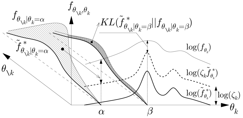
Figure 7: Illustration of Conditionally Variational approximation (CVA), as defined in (23). The lower KL divergence, the better approximation. Given initially a conditional form $\widetilde{f}_{\theta_{\backslash k}|\theta_{k}}^{*}$ for $\widetilde{f}_{\boldsymbol{\theta}}=\widetilde{f}_{\theta_{\backslash k}|\theta_{k}}^{*}\widetilde{f}_{\theta_{k}}$, the optimally approximated marginal $\widetilde{f}_{\theta_{k}}^{*}$ minimizing $\text{KL}(\widetilde{f}_{\boldsymbol{\theta}}||f_{\boldsymbol{\theta}})$ is proportional to the true marginal $f_{\theta_{k}}$ in $f_{\boldsymbol{\theta}}=f_{\theta_{\backslash k}|\theta_{k}}f_{\theta_{k}}$ by a fraction of normalized conditional divergence $\text{$\zeta$}_{k}\exp\text{KL}(\widetilde{f}_{\theta_{\backslash k}|\theta_{k}}^{*}||f_{\theta_{\backslash k}|\theta_{k}})$, where $\text{$\zeta$}_{k}$ is the normalizing constant. In traditional VB approximation (29), we simply set $\widetilde{f}_{\theta_{\backslash k}|\theta_{k}}^{*}=\widetilde{f}_{\theta_{\backslash k}}^{*}$, which is independent of $\theta_{k}$.

IV-B1 Conditionally Variational approximation (CVA)

For a good approximation $\widetilde{f}_{k}$ of $f_{k}$, let us initially pick a closed form p.d.f. $\widetilde{f}(\boldsymbol{\theta})=\widetilde{f}^{*}(\theta_{\backslash k}|\theta_{k})\widetilde{f}_{k}(\theta_{k})$, in which the conditional distribution $\widetilde{f}_{\backslash k|k}^{*}\triangleq\widetilde{f}^{*}(\theta_{\backslash k}|\theta_{k})$ is fixed and given. The optimal approximation $\widetilde{f}_{k}^{*}\triangleq\widetilde{f}_{k}^{*}(\theta_{k})$ is then found by the following Theorem, which is also the foundational idea of this paper:

Theorem 23.

(Conditionally Variational approximation)
Let $\widetilde{f}=\widetilde{f}_{\backslash k|k}^{*}\widetilde{f}_{k}$ be a family of distributions with fixed-form conditional $\widetilde{f}_{\backslash k|k}^{*}$. Then $\widetilde{f}$ is convex over marginals $\widetilde{f}_{k}$, which yields:

$$\text{KL}_{\widetilde{f}||f}=\text{KL}_{\widetilde{f}||\widetilde{f}^{*}}+\text{KL}_{\widetilde{f}^{*}||f}\geq\text{KL}_{\widetilde{f}^{*}||f}=\log\frac{1}{\zeta_{k}}$$ (22)

owing to Bregman pythagorean property (3) for functional space (9-10). The distribution $\widetilde{f}=\widetilde{f}^{*}$ minimizing $\text{KL}_{\widetilde{f}||f}$ and the value $\zeta_{k}$ in (22) are given as follows:

$$\widetilde{f}_{k}^{*}(\theta_{k}) =\frac{f_{k}(\theta_{k})}{\text{$\zeta$}_{k}\exp(\text{KL}_{\widetilde{f}_{\backslash k|k}^{*}||f_{\backslash k|k}})}$$ (23)

$$=\frac{1}{\text{$\zeta$}_{k}}\exp\mathbb{E}_{\widetilde{f}^{*}(\theta_{\backslash k}|\theta_{k})}\log\frac{f(\boldsymbol{\theta})}{\widetilde{f}^{*}(\theta_{\backslash k}|\theta_{k})}$$

in which $\zeta_{k}$ is the normalizing constant of $\widetilde{f}_{k}^{*}$ in (23) and $\text{KL}_{\widetilde{f}_{\backslash k|k}^{*}||f_{\backslash k|k}}\triangleq\text{KL}(\widetilde{f}^{*}(\theta_{\backslash k}|\theta_{k})||f(\theta_{\backslash k}|\theta_{k}))$.

Note that, if the marginal $\widetilde{f}_{k}=\widetilde{f}_{k}$ is initially fixed instead, $\widetilde{f}$ is then convex over $\widetilde{f}_{\backslash k|k}$ and, hence, the conditional $\widetilde{f}_{\backslash k|k}^{*}$ minimizing $\text{KL}_{\widetilde{f}||f}$ in (22) is the true conditional distribution $f_{\backslash k|k}$, i.e. $\widetilde{f}_{\backslash k|k}^{*}=f_{\backslash k|k}$.

Proof:

Firstly, we note that, for any mixture $\widetilde{f}_{k}(\theta_{k})=p_{1}\widetilde{f}_{1}(\theta_{k})+p_{2}\widetilde{f}_{2}(\theta_{k})$, we always have $\widetilde{f}(\boldsymbol{\theta})=p_{1}\widetilde{f}_{1}(\boldsymbol{\theta})+p_{2}\widetilde{f}_{2}(\boldsymbol{\theta})$. Hence, $\widetilde{f}$ is convex over $\widetilde{f}_{k}$ with fixed $\widetilde{f}_{\backslash k|k}$ and satisfies the Bregman pythagorean equality (22), since KL divergence is a special case of Bregman divergence (9). We can also verify the pythagorean equality (22) directly, similarly to the proof of copula’s KL divergence (21), as follows:

$$\text{$\text{KL}$}_{\widetilde{f}||f} =\mathbb{E}_{\widetilde{f}_{k}}\text{$\text{KL}$}_{\widetilde{f}_{\backslash k|k}^{*}||f_{\backslash k|k}}+\text{$\text{KL}$}_{\widetilde{f}_{k}||f_{k}}$$

$$=\mathbb{E}_{\widetilde{f}_{k}}\log\frac{\widetilde{f}_{k}}{\frac{1}{\text{$\zeta$}_{k}}\frac{f_{k}}{\exp(\text{$\text{KL}$}_{\widetilde{f}_{\backslash k|k}^{*}||f_{\backslash k|k}})}}+\mathbb{E}_{\widetilde{f}_{k}}\log\frac{1}{\text{$\zeta$}_{k}}$$

$$=\underset{\text{KL}_{\widetilde{f}||\widetilde{f}^{*}}}{\underbrace{\text{$\text{KL}$}_{\widetilde{f}_{k}||\widetilde{f}_{k}^{*}}}}+\underset{\text{KL}_{\widetilde{f}^{*}||f}}{\underbrace{\log\frac{1}{\text{$\zeta_{k}$}}}}$$ (24)

in which the form $\widetilde{f}_{k}^{*}$ is defined in (23) and $\zeta_{k}$ is independent of $\theta_{k}$. Also, we have $\text{KL}_{\widetilde{f}||\widetilde{f}^{*}}=\text{$\text{KL}$}_{\widetilde{f}_{k}||\widetilde{f}_{k}^{*}}$ in the first term of r.h.s. of (24) since $\widetilde{f}$ and $\widetilde{f}^{*}$ only differ in marginals $\widetilde{f}_{k}$, $\widetilde{f}_{k}^{*}$. For the second term, by definition (23), we have $\text{$\text{KL}$}_{\widetilde{f}_{\backslash k|k}^{*}||f_{\backslash k|k}}=\log\frac{1}{\text{$\zeta$}_{k}}\frac{f_{k}(\theta_{k})}{\widetilde{f}_{k}^{*}(\theta_{k})}$, which yields: $\mathbb{E}_{\widetilde{f}_{k}^{*}}\text{$\text{KL}$}_{\widetilde{f}_{\backslash k|k}^{*}||f_{\backslash k|k}}=\log\frac{1}{\text{$\zeta$}_{k}}-\text{$\text{KL}$}_{\widetilde{f}_{k}^{*}||f_{k}}\Leftrightarrow\text{KL}_{\widetilde{f}^{*}||f}=\log\frac{1}{\text{$\zeta$}_{k}}$ in (22) and (24). Lastly, the second equality in (23) is given as follows: $f_{k}(\theta_{k})/\exp\text{KL}_{\widetilde{f}_{\backslash k|k}^{*}||f_{\backslash k|k}}=f_{k}(\theta_{k})\exp\mathbb{E}_{\widetilde{f}_{\backslash k|k}^{*}}\log\frac{f_{\backslash k|k}}{\widetilde{f}_{\backslash k|k}^{*}}=\exp\mathbb{E}_{\widetilde{f}_{\backslash k|k}^{*}}\log\frac{f(\boldsymbol{\theta})}{\widetilde{f}_{\backslash k|k}^{*}}$.

If $\widetilde{f}_{k}=\widetilde{f}_{k}^{*}$ is fixed instead, $\widetilde{f}$ is then convex over a mixture of $\widetilde{f}_{\backslash k|k}$ as shown above. Then, $\text{$\text{KL}$}_{\widetilde{f}||f}$ in (24) is minimum at $\widetilde{f}_{\backslash k|k}^{*}=f_{\backslash k|k}$, since the term $\text{$\text{KL}$}_{\widetilde{f}_{k}||f_{k}}=\text{$\text{KL}$}_{\widetilde{f}_{k}^{*}||f_{k}}$ in (24) is now fixed and the term $\mathbb{E}_{\widetilde{f}_{k}^{*}}\text{$\text{KL}$}_{\widetilde{f}_{\backslash k|k}^{*}||f_{\backslash k|k}}$ is minimum at zero with $\widetilde{f}_{\backslash k|k}^{*}=f_{\backslash k|k}$. ∎

In Theorem 23, the conditional $\widetilde{f}_{\backslash k|k}^{*}$ is fixed beforehand and $\widetilde{f}_{k}^{*}$ is found in a free-form variational space, hence the name Conditionally Variational approximation (CVA). The case of fixed marginal $\widetilde{f}_{k}^{*}$ is not interesting, since $\text{KL}_{\widetilde{f}||f}$ in this case is only minimized at the true conditional $f_{\backslash k|k}$, which is often unknown initially.

Remark 24.

The CVA form above is a generalized form of the so-called Conditional Variational Bayesian inference [28] or Conditional mean-field [29] in literature, which are merely applications of mean-field approximations to a conditionally independent structure, i.e. $\widetilde{f}(\boldsymbol{\theta}|\xi)=\prod_{k=1}^{K}\widetilde{f}_{k}(\theta_{k}|\xi)$, given a latent variable $\xi$ in this case.

IV-B2 Copula Variational algorithm

In CVA form above, we can only find one approximated marginal $\widetilde{f}_{k}^{*}(\theta_{k})$, given conditional form $\widetilde{f}_{\backslash k|k}^{*}(\theta_{\backslash k}|\theta_{k})$. In the iterative form below, we will iteratively multiply $\widetilde{f}_{k}^{*}(\theta_{k})$ back to $\widetilde{f}_{\backslash k|k}^{*}(\theta_{\backslash k}|\theta_{k})$ in order to find the reverse conditional $\widetilde{f}_{k|\backslash k}^{*}(\theta_{k}|\theta_{\backslash k})$ for the next $\widetilde{f}_{\backslash k}^{*}(\theta_{\backslash k})$ via (23). At convergence, we can find a set of approximations $\widetilde{f}_{k}$, $\forall k\in\{1,2,\ldots,K\}$, such that the $\text{KL}_{\widetilde{f}||f}$ is locally minimized, as follows:

Corollary 25.

(Copula Variational approximation)
Let $\widetilde{f}=\widetilde{f}_{\backslash k|k}^{[0]}\widetilde{f}_{k}$ be the initial approximation with initial form $\widetilde{f}_{\backslash k|k}^{[0]}$. At iteration $\nu\in\{1,2,\ldots,\nu_{c}\}$, the approximation $\widetilde{f}^{[\nu]}=\widetilde{f}_{\backslash k|k}^{[\nu-1]}\widetilde{f}_{k}^{[\nu]}=\widetilde{f}_{k|\backslash k}^{[\nu]}\widetilde{f}_{\backslash k}^{[\nu]}$ is given by (23), as follows:

$$\widetilde{f}_{k}^{[\nu]}(\theta_{k})=\frac{f_{k}(\theta_{k})}{\zeta_{k}^{[\nu]}\exp(\text{KL}_{\widetilde{f}_{\backslash k|k}^{[\nu-1]}||f_{\backslash k|k}})}$$ (25)

in which the reverse conditional is $\widetilde{f}_{k|\backslash k}^{[\nu]}=\frac{\widetilde{f}_{\backslash k|k}^{[\nu-1]}\widetilde{f}_{k}^{[\nu]}}{\widetilde{f}_{\backslash k}^{[\nu]}}$ and $\widetilde{f}_{\backslash k}^{[\nu]}\triangleq\int_{\theta_{k}}\widetilde{f}_{\backslash k|k}^{[\nu-1]}\widetilde{f}_{k}^{[\nu]}$, $\forall k\in\{1,2,\ldots,K\}$. Then, the value $\text{KL}_{\widetilde{f}^{[\nu]}||f}=\log\frac{1}{\zeta_{k}^{[\nu]}}$ in (22), where $\zeta_{k}^{[\nu]}$ is the normalizing constant of marginal $\widetilde{f}_{k}^{[\nu]}$, monotonically decreases to a local minimum at convergence $\nu=\nu_{c}$, as illustrated in Fig. 8.

Note that, by copula’s marginal-invariant property (19), the copula’s form of the iterative joint distribution $\widetilde{f}^{[\nu]}(\boldsymbol{\theta})$ is invariant with any updated marginals $\widetilde{f}_{k}^{[\nu]}(\theta_{k})$, $\forall k$, hence the name Copula Variational approximation.

Proof:

Since the calculation of reverse form $\widetilde{f}_{k|\backslash k}^{[\nu]}$ does not change $\widetilde{f}^{[\nu]}(\boldsymbol{\theta})$, the value $\text{KL}_{\widetilde{f}^{[\nu]}||f}$ only decreases with marginal update $\widetilde{f}_{k}^{[\nu]}$ via (22-23) and, hence, converges monotonically. ∎

If the initial form $\widetilde{f}_{\backslash k|k}^{[0]}$ belongs to the independent space, i.e. $\widetilde{f}_{\backslash k|k}^{[0]}=\widetilde{f}_{\backslash k}^{[0]}$, the copula of the joint $\widetilde{f}_{\boldsymbol{\theta}}^{[0]}$ will have independent form, as noted in Remark 15, and cannot leave this independence space via dual iterations of (25). Hence, for a binary partition $\boldsymbol{\theta}=\{\theta_{\backslash k},\theta_{k}\}$, an initially independent copula will lead to a mean-field approximation.

Nonetheless, this is not true in general for ternary partition $\boldsymbol{\theta}=\{\theta_{k},\theta_{j},\theta_{m}\}$ or for a generic network of parameters, since the iterative CVA (25) can be implemented with different partitions of a network at any iteration, without changing the joint network’s copula or increasing the joint KL divergence $\text{KL}_{\widetilde{f}^{[\nu]}||f}$.

For example, in ternary partition, even if we initially set $\widetilde{f}_{k|\backslash k}^{[0]}=\widetilde{f}_{k}^{[0]}$ independent of $\theta_{\backslash k}=\{\theta_{j},\theta_{m}\}$ and yield the updated $\widetilde{f}_{\backslash k}^{[1]}=\widetilde{f}^{[1]}(\theta_{j},\theta_{m})$ for $\widetilde{f}^{[1]}=\widetilde{f}_{k}^{[0]}\widetilde{f}_{\backslash k}^{[1]}=\widetilde{f}_{m|j}^{[1]}\widetilde{f}_{\backslash m}^{[1]}$ via (25), the reverse form $\widetilde{f}_{m|j}^{[1]}$ yields $\widetilde{f}_{\backslash m}^{[2]}\triangleq\widetilde{f}^{[2]}(\theta_{k},\theta_{j})$ via (25) again and, hence $\widetilde{f}_{k|\backslash k}^{[2]}=\widetilde{f}^{[2]}(\theta_{k}|\theta_{j})$ dependent on $\theta_{j}$ again, which does not yield a mean-field approximation in subsequent iterations of (25). This ternary partition scheme will be implemented in (59) and clarified further in Remark 42.

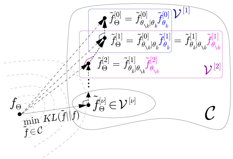
Figure 8: Venn diagram for iterative Copula Variational approximation (CVA), given in (25). The dashed contours represent the convexity of $\text{KL}(\widetilde{f}_{\boldsymbol{\theta}}||f_{\boldsymbol{\theta}})$ over distributional points $\widetilde{f}_{\boldsymbol{\theta}}$. The set $\mathcal{C}$, possibly nonconvex, denotes a class of distributions with the same copula form. Given initial form $\widetilde{f}_{\theta_{\backslash k}|\theta_{k}}^{[0]}$, the joint distributions $\widetilde{f}_{\boldsymbol{\theta}}^{[0]}$ and $\widetilde{f}_{\boldsymbol{\theta}}^{[1]}$ belong to the same convex set $\mathcal{V}^{[1]}\subseteq\mathcal{C}$, by Theorem 23 and Corollary 25. The CVA $\widetilde{f}_{\boldsymbol{\theta}}^{[1]}$ is the Bregman projection of the true distribution $f_{\boldsymbol{\theta}}$ onto $\mathcal{V}^{[1]}$, with $\widetilde{f}_{\theta_{k}}^{[1]}=\operatornamewithlimits{arg\,min}_{\widetilde{f}_{\theta_{k}}\in\mathcal{V}^{[1]}}\text{KL}(\widetilde{f}_{\boldsymbol{\theta}}||f_{\boldsymbol{\theta}})$, as shown in (22) and illustrated in Fig. 2. By interchanging the role of $\theta_{\backslash k}$ and $\theta_{k}$, the $\text{KL}(\widetilde{f}_{\boldsymbol{\theta}}^{[\nu]}||f_{\boldsymbol{\theta}})$ never increases over iterations $\nu$ and, hence, converges to a local minimum inside copula set $\mathcal{C}$. In traditional VB algorithm, we set $\widetilde{f}_{\theta_{\backslash k}|\theta_{k}}^{[\nu]}=\widetilde{f}_{\theta_{\backslash k}}^{[\nu]}$, which belongs to the independent copula class at all iterations $\nu$.

IV-B3 Conditionally exponential family (CEF) approximation

The computation in above approximations will be linearly tractable, if the true joint $f(\boldsymbol{\theta})$ and the approximated conditional $\widetilde{f}_{\backslash k|k}$ can be linearly factorized with respect to $\log$-operator in (23) and (25). The distributions satisfying this property belong to a special class of distributions, namely CEF, defined as follows:

Definition 26.

(Conditionally Exponential Family)
A joint distribution $f(\boldsymbol{\theta})$ is a member of CEF if it has the following form:

$$f(\boldsymbol{\theta})\propto\exp\left\langle\boldsymbol{g}_{k}(\theta_{k}),\boldsymbol{g}_{\backslash k}(\theta_{\backslash k})\right\rangle$$ (26)

where $\boldsymbol{g}_{k}$, $\boldsymbol{g}_{\backslash k}$ are vectors dependent on $\theta_{k}$, $\theta_{\backslash k}$ element-wise, respectively. Note that, the form (26) is similar to the well-known Exponential Family in literature [2, 45], hence the name CEF.

From (26), the marginal of a joint CEF distribution is:

$$f(\theta_{k})\propto\int_{\theta_{\backslash k}}\exp\left\langle\boldsymbol{g}_{k}(\theta_{k}),\boldsymbol{g}_{\backslash k}(\theta_{\backslash k})\right\rangle d\theta_{\backslash k}$$ (27)

which may not be tractable, since the CEF form is not factorable in general. In contrast, the CVA (23) for CEF distributions (26) is more tractable, as follows:

Corollary 27.

(CEF approximation)
Let $\widetilde{f}=\widetilde{f}_{\backslash k|k}^{*}\widetilde{f}_{k}$ be a distribution with $\widetilde{f}_{\backslash k|k}^{*}=\exp\left\langle\boldsymbol{h}_{k}(\theta_{k}),\boldsymbol{h}_{\backslash k}(\theta_{\backslash k})\right\rangle$ given by CEF form in (26). If the true distribution $f(\boldsymbol{\theta})$ also takes the CEF form (26), the approximation $\widetilde{f}^{*}$ minimizing $\text{KL}_{\widetilde{f}||f}$ in (22), as given by (23), also belongs to CEF, as follows:

$$\widetilde{f}_{k}^{*}(\theta_{k})\propto\exp\left\langle\boldsymbol{\eta}_{k}(\theta_{k}),\boldsymbol{\eta}_{\backslash k}^{*}(\theta_{k})\right\rangle$$ (28)

where $\boldsymbol{\eta}_{\backslash k}^{*}(\theta_{k})\triangleq\mathbb{E}_{\widetilde{f}_{\backslash k|k}^{*}}\boldsymbol{\eta}_{\backslash k}(\theta_{\backslash k})$, with $\boldsymbol{\eta}_{k}\triangleq\boldsymbol{g}_{k}-\boldsymbol{h}_{k}$ and $\boldsymbol{\eta}_{\backslash k}\triangleq\boldsymbol{g}_{\backslash k}-\boldsymbol{h}_{\backslash k}$.

Proof:

The form (28) is a direct consequence of (23), since both $\widetilde{f}_{\backslash k|k}^{*}$ and $f(\boldsymbol{\theta})$ in (23) now have CEF form (26). ∎

From (27-28), we can see that the integral in (27) has moved inside the non-linear $\exp$ operator in (28) and, hence, become linear and numerically tractable. Then, substituting (28) into iterative CVA (25), we can see that the iterative CVA for CEF is also tractable, since we only have to update the parameters of CEF iteratively in (28) until convergence.

Remark 28.

In the nutshell, the key advantage of KL divergence is to approximate the originally intractable arithmetic mean (27) by the tractable geometric mean in exponential domain (28), as noted in Remark 11.

IV-B4 Backward KLD and minimum-risk (MR) approximation

In above approximations, we have used the forward $\text{$\text{KL}$}_{\widetilde{f}||f}$ (22) as the approximation criterion, since the Bregman pythagorean property (3) is only valid for forward $\text{$\text{KL}$}_{\widetilde{f}||f}$. Moreover, the approximation via backward $\text{$\text{KL}$}_{f||\widetilde{f}}$ is not interesting since the minimum is only achieved with the true distributions, as shown below:

Corollary 29.

(Conditionally minimum-risk approximation)
The approximation $\widetilde{f}^{*}=\widetilde{f}_{\backslash k|k}\widetilde{f}_{k}$ minimizing backward $\text{$\text{KL}$}_{f||\widetilde{f}}$ is either $\widetilde{f}^{*}=\widetilde{f}_{\backslash k|k}^{\text{MR}}f_{k}$ or $\widetilde{f}^{*}=f_{\backslash k|k}\widetilde{f}_{k}^{\text{MR}}$ for fixed $\widetilde{f}_{\backslash k|k}^{\text{MR}}$ or fixed $\widetilde{f}_{k}^{\text{MR}}$, respectively, where $f_{k}$ and $f_{\backslash k|k}$ are the true marginal and conditional distributions.

Proof:

Similar to proof of Theorem 23, the backward form is $\text{$\text{KL}$}_{f||\widetilde{f}}=\mathbb{E}_{f_{k}}\text{$\text{KL}$}_{f_{\backslash k|k}||\widetilde{f}_{\backslash k|k}}+\text{$\text{KL}$}_{f_{k}||\widetilde{f}_{k}}$. Hence, $\text{$\text{KL}$}_{f||\widetilde{f}^{*}}$ is minimum at $\widetilde{f}_{k}^{\text{MR}}=f_{k}$ for fixed $\text{$\text{KL}$}_{f_{\backslash k|k}||\widetilde{f}_{\backslash k|k}^{\text{MR}}}$ and minimum at $\widetilde{f}_{\backslash k|k}^{\text{MR}}=f_{\backslash k|k}$ for fixed $\text{$\text{KL}$}_{f_{k}||\widetilde{f}_{k}^{\text{MR}}}$. ∎

Remark 30.

The Corollary 29 is the generalized form of the minimum-risk approximation in [2], which minimizes backward KL divergence in the context of VB approximation in mean-field theory. The name “minimum-risk” refers to the fact that the true distribution always yields minimum-risk estimation in Bayesian theory (c.f. Appendix A).

IV-C Mean-field approximations

If we confine the conditional form $\widetilde{f}=\widetilde{f}_{\backslash k|k}\widetilde{f}_{k}$ in above approximations by independent form, i.e. $\widetilde{f}=\widetilde{f}_{\backslash k}\widetilde{f}_{k}$, we will recover the so-called mean-field approximations in literature. Four cases of them, namely VB, EM, ICM and k-means algorithms, will be presented below.

IV-C1 Variational Bayes (VB) algorithm

From CVA (23), the VB algorithm is given as follows:

Corollary 31.

(VB approximation)
The independent distribution $\widetilde{f}^{*}=\widetilde{f}_{\backslash k}^{*}\widetilde{f}_{k}^{*}$ minimizing $\text{KL}_{\widetilde{f}||f}$ in (22) is given by (23), as follows:

$$\widetilde{f}_{k}^{*}(\theta_{k}) \propto\frac{f_{k}(\theta_{k})}{\exp(\text{KL}_{\widetilde{f}_{\backslash k}^{*}||f_{\backslash k|k}})}\propto\exp\mathbb{E}_{\widetilde{f}_{\backslash k}^{*}(\theta_{\backslash k})}\log f(\boldsymbol{\theta}),$$ (29)

$\forall k\in\{1,2,\ldots,K\}$, as illustrated in Fig. 7.

Proof:

Since $\widetilde{f}_{\backslash k|k}=\widetilde{f}_{\backslash k}$ does not depends on $\theta_{k}$ in this case, substituting $\widetilde{f}_{\backslash k|k}=\widetilde{f}_{\backslash k}$ into (23) yields (29). ∎

Since there is no conditional form $\widetilde{f}_{\backslash k|k}$ to be updated, the iterative VB algorithm simply updates (29) iteratively for all marginals $\widetilde{f}_{k}$ and $\widetilde{f}_{\backslash k}$, similar to (25), until convergence. Hence, VB algorithm is a special case of Copula Variational algorithm in Corollary 25, in which the approximated copula is of independent form, as noted in Remark 15.

IV-C2 Expectation-Maximization (EM) algorithm

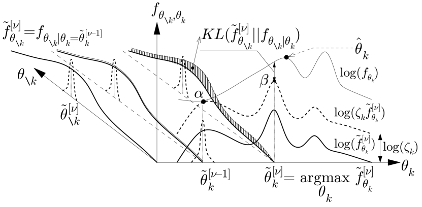
Figure 9: Illustration of Expectation-Maximization (EM) algorithm (30) as a special case of VB approximation. The lower KL divergence, the better approximation. Given restricted form $\widetilde{f}_{\theta_{\backslash k}}^{[\nu]}=f(\theta_{\backslash k}|\widetilde{\theta}_{k}^{[\nu-1]})$ at iteration $\nu$, the approximated $\widetilde{f}_{\theta_{k}}^{[\nu]}$ minimizing $\text{KL}(\widetilde{f}_{\theta_{\backslash k}}^{[\nu]}\widetilde{f}_{\theta_{k}}^{[\nu]}||f_{\boldsymbol{\theta}})$ is proportional to the true marginal $f_{\theta_{k}}$ by a fraction of conditional divergence, similar to Fig. 7. Note that, $\widetilde{\theta}_{k}^{[\nu]}$ might fail to converge to a local mode $\widehat{\theta}_{k}$ of the true marginal $f_{\theta_{k}}$, if the peak $\beta$ is lower than point $\alpha$. For ICM algorithm (31), we further restrict $\widetilde{f}_{\theta_{\backslash k}}^{[\nu]}$ to a Dirac delta distribution concentrating around its mode $\widetilde{\theta}_{\backslash k}^{[\nu]}$ and, hence, $\tilde{\boldsymbol{\theta}}^{[\nu]}=\{\widetilde{\theta}_{\backslash k}^{[\nu]},\widetilde{\theta}_{k}^{[\nu]}\}$ always converges to a joint local mode $\widehat{\boldsymbol{\theta}}$ of the true distribution $f_{\boldsymbol{\theta}}$.

If we restrict the independent form $\widetilde{f}=\widetilde{f}_{\backslash k}\widetilde{f}_{k}$ in VB algorithm with Dirac delta form $\widetilde{f}_{\text{EM}}\triangleq\widetilde{f}_{\backslash k}\widetilde{\delta}_{k}$, where $\widetilde{\delta}_{k}\triangleq\delta(\theta_{k}-\widetilde{\theta}_{k})$, we will recover the EM algorithm, as follows:

Corollary 32.

(EM algorithm)
At iteration $\nu\in\{1,2,\ldots,\nu_{c}\}$, the EM approximation of $f(\boldsymbol{\theta})$ is $\widetilde{f}_{\text{EM}}^{[\nu]}\triangleq\widetilde{f}_{\backslash k}^{[\nu]}\widetilde{\delta}_{k}^{[\nu]}$, in which $\widetilde{f}_{\backslash k}^{[\nu]}=f(\theta_{\backslash k}|\widetilde{\theta}_{k}^{[\nu]})$ and $\widetilde{\delta}_{k}^{[\nu]}\triangleq\delta(\theta_{k}-\widetilde{\theta}_{k}^{[\nu]})$, as given by (29):

$$\widetilde{\theta}_{k}^{[\nu]} \triangleq\operatornamewithlimits{arg\,max}_{\theta_{k}}\widetilde{f}_{k}^{[\nu]}(\theta_{k})=\operatornamewithlimits{arg\,max}_{\theta_{k}}\mathbb{E}_{f(\theta_{\backslash k}|\widetilde{\theta}_{k}^{[\nu-1]})}\log f(\boldsymbol{\theta})$$ (30)

$$=\operatornamewithlimits{arg\,max}_{\theta_{k}}\frac{f_{k}(\theta_{k})}{\exp(\text{KL}_{f(\theta_{\backslash k}|\widetilde{\theta}_{k}^{[\nu-1]})||f(\theta_{\backslash k}|\theta_{k})})}.$$

If $\widetilde{\theta}_{k}^{[\nu]}$ converges to a true local maximum $\widehat{\theta}_{k}$ of the original marginal $f_{k}(\theta_{k})$, as illustrated in Fig. 9, then $\text{KL}_{\widetilde{f}_{\text{EM}}^{[\nu]}||f}=-\log f_{k}(\widetilde{\theta}_{k}^{[\nu]})$ converges to a local minimum.

Proof:

Substituting the Dirac delta function $\widetilde{f}_{k}^{*}(\theta_{k})=\delta(\theta_{k}-\widetilde{\theta}_{k}^{[\nu-1]})$ to VB approximation (29), we have $\widetilde{f}_{\backslash k}^{[\nu-1]}(\theta_{\backslash k})=f(\theta_{\backslash k}|\widetilde{\theta}_{k}^{[\nu-1]})$, which yields (30) owing to (29).

Since the KL value in (30) is never negative, we have $g(\theta_{k})\triangleq f_{k}(\theta_{k})/\exp(\text{KL}_{f(\theta_{\backslash k}|\widetilde{\theta}_{k}^{[\nu-1]})||f(\theta_{\backslash k}|\theta_{k})})\leq f_{k}(\theta_{k})$ and the equality $g(\widetilde{\theta}_{k}^{[\nu]})=f_{k}(\widetilde{\theta}_{k}^{[\nu]})$ happens at $\theta_{k}=\widetilde{\theta}_{k}^{[\nu]}$, which means: $f_{k}(\widetilde{\theta}_{k}^{[\nu-1]})=g(\widetilde{\theta}_{k}^{[\nu-1]})\leq g(\widetilde{\theta}_{k}^{[\nu]})=\max g(\theta_{k})\leq\max f_{k}(\theta_{k})$. Then, as illustrated in Fig. 9, if $\widetilde{f}_{k}^{[\nu]}(\widetilde{\theta}_{k}^{[\nu]})$ strictly increases over $\nu$, $\widetilde{\theta}_{k}^{[\nu]}$ will converge to a local mode $\widehat{\theta}_{k}$ of $f_{k}(\theta_{k})$, owing to majorization-maximization (MM) principle [21, 22]. Otherwise, $\widetilde{\theta}_{k}^{[\nu]}$ might fail to converge to $\widehat{\theta}_{k}$.

Lastly, from (24), we have: $\text{KL}_{\widetilde{f}_{\text{EM}}^{[\nu]}||f}=\mathbb{E}_{\widetilde{\delta}_{k}^{[\nu]}}\text{KL}_{f(\theta_{\backslash k}|\widetilde{\theta}_{k}^{[\nu]})||f(\theta_{\backslash k}|\theta_{k})}+\text{$\text{KL}$}_{\widetilde{\delta}_{k}^{[\nu]}||f_{k}}=\text{$\text{KL}$}_{\widetilde{\delta}_{k}^{[\nu]}||f_{k}}=-\log f_{k}(\widetilde{\theta}_{k}^{[\nu]})$ by sifting property of Dirac delta function. ∎

From (29-30), we can see that EM algorithm is a special case of VB algorithm. Both of them minimizes the KL divergence within the independent distribution space, namely mean-field space.

Since EM algorithm is a fixed-form approximation, it has low computational complexity. Nonetheless, as illustrated in Fig. 9, the point estimate $\widetilde{\theta}_{k}^{[\nu]}$ in EM algorithm (30) might fail to converge to a local mode $\widehat{\theta}_{k}$ of true marginal $f_{k}(\theta_{k})$ in practice. In contrast, VB approximation is a free-form distribution and capable of approximating higher-order moments of true marginal $f_{k}(\theta_{k})$.

Remark 33.

Note that, EM algorithm is also a special case of Copula Variational algorithm (25) in conditional space. Indeed, if the marginal $\widetilde{f}_{k}$ of $\widetilde{f}=\widetilde{f}_{\backslash k|k}\widetilde{f}_{k}$ in (25) is restricted to Dirac delta form, i.e. $\widetilde{f}_{k}=\widetilde{\delta}_{k}$, the joint $\widetilde{f}$ will become a degenerated independent distribution, i.e. $\widetilde{f}=\widetilde{f}(\theta_{\backslash k}|\theta_{k}=\widetilde{\theta}_{k})\delta(\theta_{k}-\widetilde{\theta}_{k})=\widetilde{f}_{\backslash k}\widetilde{\delta}_{k}$, owing to sifting property of Dirac delta. Hence, EM algorithm is a very special approximation, since it belongs to both mean-field and copula-field approximations.

IV-C3 Iterative conditional mode (ICM) algorithm

If we further restrict the independent form $\widetilde{f}=\widetilde{f}_{\backslash k}\widetilde{f}_{k}$ in VB algorithm fully to Dirac delta form $\widetilde{f}_{\text{ICM}}\triangleq\widetilde{\delta}_{\backslash k}\widetilde{\delta}_{k}$, we will recover the iterative plug-in algorithm, also called Iterative Conditional Mode (ICM) in literature [23, 24], as follows:

Corollary 34.

(ICM algorithm)
At iteration $\nu\in\{1,2,\ldots,\nu_{c}\}$, the ICM approximation of $f(\boldsymbol{\theta})$ is $\widetilde{f}_{\text{ICM}}^{[\nu]}\triangleq\widetilde{f}_{\backslash k}^{[\nu]}\widetilde{f}_{k}^{[\nu]}=\widetilde{\delta}_{\backslash k}^{[\nu]}\widetilde{\delta}_{k}^{[\nu]}$, where $\widetilde{\delta}_{\backslash k}^{[\nu]}\triangleq\delta(\theta_{\backslash k}-\widetilde{\theta}_{\backslash k}^{[\nu]})$ and $\widetilde{\delta}_{k}^{[\nu]}\triangleq\delta(\theta_{k}-\widetilde{\theta}_{k}^{[\nu]})$ is given by (29), as follows:

$$\widetilde{\theta}_{k}^{[\nu]} \triangleq\operatornamewithlimits{arg\,max}_{\theta_{k}}f(\theta_{k}|\widetilde{\theta}_{\backslash k}^{[\nu-1]})=\operatornamewithlimits{arg\,max}_{\theta_{k}}f(\theta_{k},\theta_{\backslash k}=\widetilde{\theta}_{\backslash k}^{[\nu-1]})$$ (31)

$$\widetilde{\theta}_{\backslash k}^{[\nu]} \triangleq\operatornamewithlimits{arg\,max}_{\theta_{\backslash k}}f(\theta_{\backslash k}|\widetilde{\theta}_{k}^{[\nu]})=\operatornamewithlimits{arg\,max}_{\theta_{\backslash k}}f(\theta_{k}=\widetilde{\theta}_{k}^{[\nu]},\theta_{\backslash k})$$

From (31), we can see that $\tilde{\boldsymbol{\theta}}^{[\nu]}=\{\widetilde{\theta}_{\backslash k}^{[\nu]},\widetilde{\theta}_{k}^{[\nu]}\}$ iteratively converges to a local maximum $\hat{\boldsymbol{\theta}}$ of the true distribution $f(\boldsymbol{\theta})$ and, hence, $\text{KL}_{\widetilde{f}_{\text{ICM}}^{[\nu]}||f}=-\log f(\tilde{\boldsymbol{\theta}}^{[\nu]})$ converges to a local minimum.

Proof:

The proof is a straight-forward derivation from either VB (29) or EM (30) algorithms, by sifting property of Dirac delta forms $\widetilde{f}_{\backslash k}^{[\nu]}=\delta(\theta_{\backslash k}-\widetilde{\theta}_{\backslash k}^{[\nu]})$ and $\widetilde{f}_{k}^{[\nu]}=\delta(\theta_{k}-\widetilde{\theta}_{k}^{[\nu]})$. ∎

Since we merely plug the value $\{\widetilde{\theta}_{\backslash k}^{[\nu]},\widetilde{\theta}_{k}^{[\nu]}\}$ into the true distribution $f(\boldsymbol{\theta})$ iteratively in (31) until it reaches a local maximum, the performance of this naive hit-or-miss approach is strongly influenced by the initial points $\{\widetilde{\theta}_{\backslash k}^{[0]},\widetilde{\theta}_{k}^{[0]}\}$. Hence it is often used in practice when very low computational complexity is required or when the true distribution $f(\boldsymbol{\theta})$ does not have tractable CEF form (26).

Remark 35.

Similar to the Remark 33, we can see that ICM is a degenerated form of VB, EM and Copula Variational approximations, owing to its very simple form (31).

IV-C4 K-means algorithm

In section VI-B1, we will show that the popular k-means algorithm is equivalent to ICM algorithm being applied to a mixture of independent Gaussian distributions. Hence, k-means is also a member of mean-field approximations.

IV-D Copula Variational Bayes (CVB) approximation

In a model with unknown multi-parameters $\boldsymbol{\theta}=\{\theta_{k},\theta_{\backslash k}\}$, the minimum-risk estimation of $\theta_{k}$ can be evaluated from the marginal posterior $f(\theta_{k}|\boldsymbol{x})=\int_{\theta_{\backslash k}}f(\boldsymbol{\theta}|\boldsymbol{x})d\theta_{\backslash k}$ (c.f. Appendix A), in which the posterior distribution $f(\boldsymbol{\theta}|\boldsymbol{x})$ is then given via Bayes’ rule: $f(\boldsymbol{\theta}|\boldsymbol{x})\propto f(\boldsymbol{x},\boldsymbol{\theta})=f(\boldsymbol{x}|\boldsymbol{\theta})f(\boldsymbol{\theta})$. In practice, however, the computational complexity of the normalizing constant of $f(\boldsymbol{\theta}|\boldsymbol{x})$ involves all possible values of $\boldsymbol{\theta}$ and typically grows exponentially with number of data’s dimension, which is termed the curse of dimensionality [7]. Then, without normalizing constant of $f(\boldsymbol{\theta}|\boldsymbol{x})$, the computation of moments of $f(\theta_{k}|\boldsymbol{x})$ is also intractable.

In this subsection, we will apply both copula-field and mean-field approximations to the joint posterior distribution $f(\boldsymbol{\theta}|\boldsymbol{x})\propto f(\boldsymbol{x},\boldsymbol{\theta})$ and, then, return all marginal approximations $\widetilde{f}(\theta_{k}|\boldsymbol{x})$ directly from the joint model $f(\boldsymbol{x},\boldsymbol{\theta})$, without computing the normalizing constant of $f(\boldsymbol{\theta}|\boldsymbol{x})$, as explained below.

Corollary 36.

(Copula Variational Bayes algorithm)
At iteration $\nu\in\{1,2,\ldots,\nu_{c}\}$, the CVB approximation $\widetilde{f}^{[\nu]}(\boldsymbol{\theta}|\boldsymbol{x})=\widetilde{f}^{[\nu-1]}(\theta_{\backslash k}|\theta_{k},\boldsymbol{x})\widetilde{f}_{k}^{[\nu]}(\theta_{k}|\boldsymbol{x})$ for the joint posterior $f(\boldsymbol{\theta}|\boldsymbol{x})$ is given by (23) and (25), as follows:

$$\widetilde{f}_{k}^{[\nu]}(\theta_{k}|\boldsymbol{x}) =\frac{1}{\zeta_{k}^{[\nu]}(\boldsymbol{x})}\frac{f(\theta_{k}|\boldsymbol{x})}{\text{KL}(\widetilde{f}^{[\nu-1]}(\theta_{\backslash k}|\theta_{k},\boldsymbol{x})||f(\theta_{\backslash k}|\theta_{k},\boldsymbol{x}))}$$ (32)

$$=\frac{1}{\zeta_{k}^{[\nu]}(\boldsymbol{x})}\exp\mathbb{E}_{\widetilde{f}^{[\nu-1]}(\theta_{\backslash k}|\theta_{k},\boldsymbol{x})}\log\frac{f(\boldsymbol{x},\boldsymbol{\theta})}{\widetilde{f}^{[\nu-1]}(\theta_{\backslash k}|\theta_{k},\boldsymbol{x})}$$

in which $\widetilde{f}^{[\nu]}(\theta_{k}|\theta_{\backslash k},\boldsymbol{x})=\widetilde{f}^{[\nu]}(\boldsymbol{\theta}|\boldsymbol{x})/\widetilde{f}_{\backslash k}^{[\nu]}(\theta_{\backslash k}|\boldsymbol{x})$, $\forall k\in\{1,2,\ldots,K\}$. For stopping rule, the evidence lower bound (ELBO) for CVB is defined similarly to (22), as follows: $\text{KL}_{\widetilde{f}^{[\nu]}||f}=-\text{ELBO}^{[\nu]}+\log f(\boldsymbol{x})\geq 0$, i.e. we have:

$$\log f(\boldsymbol{x})\geq\text{ELBO}^{[\nu]}\triangleq-\text{KL}_{\widetilde{f}^{[\nu]}(\boldsymbol{\theta}|\boldsymbol{x})||f(\boldsymbol{x},\boldsymbol{\theta})}=\log\zeta_{k}^{[\nu]}(\boldsymbol{x})$$ (33)

Since the evidence $f(\boldsymbol{x})$ is a constant, $\text{$\text{KL}$}_{\widetilde{f}^{[\nu]}||f}\triangleq\text{$\text{KL}$}_{\widetilde{f}^{[\nu]}(\boldsymbol{\theta}|\boldsymbol{x})||f(\boldsymbol{\theta}|\boldsymbol{x})}$ monotonically decreases to a local minimum, while the marginal normalizing constant $\zeta_{k}^{[\nu]}(\boldsymbol{x})$ in (32) and $\text{ELBO}^{[\nu]}$ in (33) monotonically increase to a local maximum at convergence $\nu=\nu_{c}$.

Note that, the copula’s form of the iterative CVB $\widetilde{f}^{[\nu]}(\boldsymbol{\theta}|\boldsymbol{x})$ is invariant with any updated marginal $\widetilde{f}_{k}^{[\nu]}(\theta_{k}|\boldsymbol{x})$, $\forall k\in\{1,2,\ldots,K\}$, as shown in (19), hence the name Copula Variational Bayes approximation.

Proof:

Firstly, we have $\text{KL}_{\widetilde{f}^{[\nu]}(\boldsymbol{\theta}|\boldsymbol{x})||f(\boldsymbol{x},\boldsymbol{\theta})}=\text{$\text{KL}$}_{\widetilde{f}^{[\nu]}||f}-\log f(\boldsymbol{x})$ by definition of KL divergence (9), hence the definition of $\text{ELBO}^{[\nu]}$ in (33). Then, similar to (24), the value $\text{$\text{KL}$}_{\widetilde{f}||f}\triangleq\text{$\text{KL}$}_{\widetilde{f}(\boldsymbol{\theta}|\boldsymbol{x})||f(\boldsymbol{\theta}|\boldsymbol{x})}$ for arbitrary $\widetilde{f}$ in this case is:

$$\text{$\text{KL}$}_{\widetilde{f}||f}=\underset{-\text{ELBO}}{\underbrace{\text{$\text{KL}$}_{\widetilde{f}_{k}||\widetilde{f}_{k}^{[\nu]}}+\log\frac{1}{\text{$\zeta_{k}^{[\nu]}$($\boldsymbol{x}$)}}}}+\log f(\boldsymbol{x}),$$ (34)

in which $\widetilde{f}_{k}^{[\nu]}$ is defined in 32, the form $f(\boldsymbol{\theta})$ in (24) is now replaced by $f(\boldsymbol{\theta}|\boldsymbol{x})=f(\boldsymbol{x},\boldsymbol{\theta})/f(\boldsymbol{x})$, hence the term $f(\boldsymbol{x},\boldsymbol{\theta})$ in (32) and the constant evidence $\log f(\boldsymbol{x})$ in (34). Since $\text{$\text{KL}$}_{\widetilde{f}_{k}||\widetilde{f}_{k}^{[\nu]}}=0$ for the case $\widetilde{f}_{k}=\widetilde{f}_{k}^{[\nu]}$, the value ELBO in (34) is equal to $\log\zeta_{k}^{[\nu]}(\boldsymbol{x})$, which yields (33). The rest of proof is similar to the proof of Corollary 25. ∎

Note that, CVB algorithm (32) is essentially the same as the Copula Variational algorithm in (25). The key difference is that the former is applied to a joint posterior $f(\boldsymbol{\theta}|\boldsymbol{x})$, while the latter is applied to a joint distribution $f(\boldsymbol{\theta})$. Hence, in CVB, the joint model $f(\boldsymbol{x},\boldsymbol{\theta})$ and ELBO (33) are preferred, since the evidence $\log f(\boldsymbol{x})$ is often hard to compute in practice. Nevertheless, for notational simplicity, let us call both of them CVB hereafter. By this way, the name CVA (23) also implies that it is the first step of CVB algorithm.

Remark 37.

Although the iterative CVB form (32) is novel, the definition of ELBO via KL divergence in (33) was recently proposed in [32]. Nevertheless, the value $\log\zeta_{k}^{[\nu]}(\boldsymbol{x})$ of ELBO in (33) was not given therein. Also, the so-called copula variational inference in [32] was to locally minimize ELBO (33) via a sampling-based stochastic-gradient decent for copula’s parameters, rather than via a deterministic expectation operator in (32). No explicit CVB’s marginal form at convergence was given in [32].

IV-D1 Conditionally Exponential Family (CEF) for posterior distribution

Similar to (28), the computation of CVB algorithm (32) will be linearly tractable if the true posterior $f(\boldsymbol{\theta}|\boldsymbol{x})$ belongs to CEF (26), as follows:

$$f(\boldsymbol{\theta}|\boldsymbol{x})\propto f(\boldsymbol{x},\boldsymbol{\theta})=\frac{1}{Z}\exp\left\langle\boldsymbol{g}_{k}(\theta_{k},\boldsymbol{x}),\boldsymbol{g}_{\backslash k}(\theta_{\backslash k},\boldsymbol{x})\right\rangle.$$ (35)

Since $Z$ is merely a normalizing constant in (35), we can also replace $f(\boldsymbol{x},\boldsymbol{\theta})$ in CVB algorithm (32) by its unnormalized form $q(\boldsymbol{x},\boldsymbol{\theta})\triangleq\exp\left\langle\boldsymbol{g}_{k},\boldsymbol{g}_{\backslash k}\right\rangle$ in (35). Since the parameters $\theta_{k}$ and $\theta_{\backslash k}$ in (35) are separable, the CVB form (28) is tractable and conjugate to the original distribution (35). For this reason, the CEF form (35) was also called the conditionally conjugate model for exponential family [46], the conjugate-exponential class [3] or the separable-in-parameter family [2] in mean-field context.

IV-D2 Mean-field approximations for posterior distribution

Similar to CVB (32), the mean-field algorithms in section IV-C can be applied to the posterior $f(\boldsymbol{\theta}|\boldsymbol{x})$, except that the original joint distribution $f(\boldsymbol{\theta})$ in those mean-field algorithms is now replaced by the joint model $f(\boldsymbol{x},\boldsymbol{\theta})$. By this way, the EM and ICM algorithms are also able to return a local maximum-a-posteriori (MAP) estimate of the true marginal $f(\theta_{k}|\boldsymbol{x})$ and the true joint $f(\boldsymbol{\theta}|\boldsymbol{x})$, respectively, either directly from joint model $f(\boldsymbol{x},\boldsymbol{\theta})$ or indirectly from its unnormalized form $q(\boldsymbol{x},\boldsymbol{\theta})$.

In literature, there are three main approaches for proof of VB approximation (29) when applied to the joint model $f(\boldsymbol{x},\boldsymbol{\theta})$ in (32), as briefly summarized below. All VB’s proofs were, however, confined within independent space $\widetilde{f}=\widetilde{f}_{\backslash k}\widetilde{f}_{k}$ and, hence, did not yield the CVB form (32):

• The first approach (e.g. in [2, 47, 48]) is to expand $\text{$\text{KL}$}_{\widetilde{f}||f}$ directly, i.e. similar to CVA’s proof (24).

• The second approach (e.g. in [11, 49]) is to start with Jensen’s inequality for the so-called energy [50, 12]: $\log Z(\boldsymbol{x})=\log\mathbb{E}_{\widetilde{f}(\boldsymbol{\theta})}\frac{q(\boldsymbol{x},\boldsymbol{\theta})}{\widetilde{f}(\boldsymbol{\theta})}\geq\mathbb{E}_{\widetilde{f}(\boldsymbol{\theta})}\log\frac{q(\boldsymbol{x},\boldsymbol{\theta})}{\widetilde{f}(\boldsymbol{\theta})}$, which is equivalent to the ELBO’s inequality in (33), since the term $Z(\boldsymbol{x})\triangleq\int_{\boldsymbol{\theta}}q(\boldsymbol{x},\boldsymbol{\theta})d\boldsymbol{\theta}$ is proportional to $f(\boldsymbol{x})$, i.e. $f(\boldsymbol{x})=\int_{\boldsymbol{\theta}}f(\boldsymbol{x},\boldsymbol{\theta})d\boldsymbol{\theta}=\frac{1}{Z}\int_{\boldsymbol{\theta}}q(\boldsymbol{x},\boldsymbol{\theta})d\boldsymbol{\theta}=\frac{Z(\boldsymbol{x})}{Z}$, owing to (35). Note that, the Jensen’s inequality is merely a consequence of Bregman variance theorem, of which KL divergence is a special case, as shown in Theorem 5.

• The third approach (e.g. in [3, 4]) is to derive the functional derivative of $\text{$\text{KL}$}_{\widetilde{f}||f}$ via Lagrange multiplier in calculus of variations (hence the name “variational” in VB). In this paper, however, the Bregman pythagorean projection for functional space (3, 10) was applied instead and it gave a simpler proof for CVA (22) and VB (29), since the gradient form of Bregman divergence in (2) is more concise than traditional functional derivative.

In practice, since the evidence $f(\boldsymbol{x})$ is hard to compute, the ELBO term in (33) was originally defined as a feasible stopping rule for iterative VB algorithm [46]. The ELBO for CVB in (33), computed via conditional form $\widetilde{f}_{\backslash k|k}^{[\nu-1]}$ in (32), can also be used as a stopping rule for CVB algorithm.

Figure 10: Augmented CVB approximation $\widetilde{f}_{0}(\boldsymbol{\theta})$ for a complicated joint distribution $f(\boldsymbol{\theta})$, illustrated via directed acyclic graphs (DAG). Each $\widetilde{f}_{i}(\boldsymbol{\theta})$ is a converged CVB approximation of $f(\boldsymbol{\theta})$ with simpler structure. The weight vector $\widetilde{\boldsymbol{p}}\triangleq[\widetilde{p}{}_{1},\widetilde{p}{}_{2},\ldots,\widetilde{p}_{N}]^{T}$, with $\sum_{i=1}^{N}\widetilde{p}_{i}=1$, is then calculated via (38) and yields the optimal mixture $\widetilde{f}_{0}(\boldsymbol{\theta})\triangleq\sum_{i=1}^{N}\widetilde{p}_{i}\widetilde{f}_{i}(\boldsymbol{\theta})$ minimizing the upper bounds (39-40) of $\text{KL}_{\widetilde{f}_{0}||f}$. Since $\text{KL}_{\widetilde{f}_{0}||f}$ is convex over $\widetilde{f}_{0}$, the mixture $\widetilde{f}_{0}$ would be close to the original $f$, if we can design a set of $\widetilde{f}_{i}$ such that $f$ stays inside a polytope bounded by vertices $\widetilde{f}_{i}$, as illustrated in Fig. 4. Hence, a good choice of $\widetilde{f}_{i}$ might be a set of overlapped sectors of the original network $f$, such that its mixture would have a similar structure of $f$, as illustrated in above DAGs.

V Hierarchical CVB for Bayesian network

In this section, let us apply the CVB approximation to a joint posterior $f(\boldsymbol{\theta}|\boldsymbol{x})$ of a generic Bayesian network. Since the network structure of $f(\boldsymbol{\theta}|\boldsymbol{x})$ is often complicated in practice, an intuitive approach is to approximate $f(\boldsymbol{\theta}|\boldsymbol{x})$ with a simpler CEF structure $\widetilde{f}(\boldsymbol{\theta}|\boldsymbol{x})$, such that the $\text{KL}_{\widetilde{f}||f}$ can be locally minimized via iterative CVB algorithm.

Nevertheless, since CVB approximation $\widetilde{f}^{[\nu]}(\boldsymbol{\theta}|\boldsymbol{x})$ in (32) cannot change its copula form at any iteration $\nu$, a natural approach is to design initially a set of simple network structures $\widetilde{f}_{i}^{[0]}$, $i\in\{1,2,\ldots,N\}$, and then combine them into a more complex structure with lowest $\text{KL}_{\widetilde{f}^{[\nu_{c}]}||f}$, or equivalently, highest ELBO (33) at convergence $\nu=\nu_{c}$. An augmented hierarchy method for merging potential CVB’s structures, as illustrated in Fig. 10, will be studied below.

For simplicity, let us consider the case of joint distribution $f(\boldsymbol{\theta})$ first, before applying the augmented approach to joint posterior $f(\boldsymbol{\theta}|\boldsymbol{x})$.

V-A Augmented CVB for mixture model

Let us firstly consider a mixture model, which is the simplest structure of a hierarchical network. The traditional mixture $f(\boldsymbol{\theta}|\boldsymbol{p})=\sum_{i=1}^{N}p_{i}f_{i}(\boldsymbol{\theta})=\sum_{\boldsymbol{l}}f(\boldsymbol{\theta},\boldsymbol{l}|\boldsymbol{p})$ and its approximation $\widetilde{f}(\boldsymbol{\theta}|\widetilde{\boldsymbol{p}})=\sum_{i=1}^{N}\widetilde{p}_{i}\widetilde{f}_{i}(\boldsymbol{\theta})=\sum_{\boldsymbol{l}}\widetilde{f}(\boldsymbol{\theta},\boldsymbol{l}|\widetilde{\boldsymbol{p}})$ can be written in augmented form via a boolean label vector $\boldsymbol{l}\triangleq[l{}_{1},l{}_{2},\ldots,l_{N}]^{T}\in\mathbb{I}^{N}$, as follows:

$$f(\boldsymbol{\theta},\boldsymbol{l}|\boldsymbol{p}) =f(\boldsymbol{\theta}|\boldsymbol{l})f(\boldsymbol{l}|\boldsymbol{p})=\prod_{i=1}^{N}f_{i}^{l{}_{i}}(\boldsymbol{\theta})p_{i}^{l{}_{i}},$$ (36)

$$\widetilde{f}(\boldsymbol{\theta},\boldsymbol{l}|\widetilde{\boldsymbol{p}}) =\widetilde{f}(\boldsymbol{\theta}|\boldsymbol{l})\widetilde{f}(\boldsymbol{l}|\widetilde{\boldsymbol{p}})=\prod_{i=1}^{N}\widetilde{f}_{i}^{l{}_{i}}(\boldsymbol{\theta})\widetilde{p}_{i}^{l{}_{i}},$$

where $\boldsymbol{l}\in\{\boldsymbol{\epsilon}{}_{1},\boldsymbol{\epsilon}{}_{2},\ldots,\boldsymbol{\epsilon}_{N}\}$ and $\boldsymbol{\epsilon}_{i}\triangleq[0,\ldots,1,\ldots 0]^{T}$ is a $N\times 1$ element vector with all zero elements except the unit value at $i$-th position, $\forall i\in\{1,2,\ldots,N\}$. Each $\widetilde{f}_{i}$ is then assumed to be the converged CVB approximation of each original component $f_{i}$.

Ideally, our aim is to pick the weight vector $\widetilde{\boldsymbol{p}}\triangleq[\widetilde{p}{}_{1},\widetilde{p}{}_{2},\ldots,\widetilde{p}_{N}]^{T}$ such that $\text{KL}(\widetilde{f}(\boldsymbol{\theta}|\widetilde{\boldsymbol{p}})||f(\boldsymbol{\theta}|\boldsymbol{p}))$ is minimized. Nevertheless, it is not feasible to directly factorize the mixture form $f(\boldsymbol{\theta}|\boldsymbol{p})$ and $\widetilde{f}(\boldsymbol{\theta}|\widetilde{\boldsymbol{p}})$ via non-linear form of KL divergence. Instead, let us minimize the KL divergence of their augmented forms in (36), as follows:

$$\widetilde{\boldsymbol{p}}^{*}\triangleq\operatornamewithlimits{arg\,min}_{\widetilde{\boldsymbol{p}}}\text{KL}(\widetilde{f}(\boldsymbol{\theta},\boldsymbol{l}|\widetilde{\boldsymbol{p}})||f(\boldsymbol{\theta},\boldsymbol{l}|\boldsymbol{p})),$$ (37)

which is also an upper bound of $\text{KL}(\widetilde{f}(\boldsymbol{\theta}|\widetilde{\boldsymbol{p}})||f(\boldsymbol{\theta}|\boldsymbol{p}))$, as shown in (21). The solution for (37) can be found via CVA (23), as follows:

Corollary 38.

(CVA for mixture model)
Applying CVA (23) to (37), we can compute the optimal weight $\widetilde{\boldsymbol{p}}^{*}\triangleq[\widetilde{p}^{*}{}_{1},\widetilde{p}^{*}{}_{2},\ldots,\widetilde{p}^{*}_{N}]^{T}$ minimizing (37), as follows:

$$\widetilde{p}_{i}^{*}\propto\frac{p_{i}}{\exp(\text{$\text{KL}$}_{\widetilde{f}_{i}||f_{i}})},\ \forall i\in\{1,2,\ldots,N\}.$$ (38)

From (24), the minimum value of (37) is then:

$$\text{KL}_{\widetilde{\boldsymbol{p}}^{*}}\triangleq\sum_{i=1}^{N}\widetilde{p}_{i}^{*}\text{$\text{KL}$}_{\widetilde{f}_{i}||f_{i}}+\sum_{i=1}^{N}\widetilde{p}_{i}^{*}\log\frac{p_{i}}{\widetilde{p}_{i}^{*}}$$ (39)

Proof:

From CVA (23), the marginal $\widetilde{f}(\boldsymbol{l}|\widetilde{\boldsymbol{p}})$ minimizing (37) is $\widetilde{f}(\boldsymbol{l}|\widetilde{\boldsymbol{p}})\propto f(\boldsymbol{l}|\boldsymbol{p})/\exp(\text{$\text{KL}$}(\widetilde{f}(\boldsymbol{\theta}|\boldsymbol{l})||f(\boldsymbol{\theta}|\boldsymbol{l}))$, which yields (38), since $\text{$\text{KL}$}(\widetilde{f}(\boldsymbol{\theta}|\boldsymbol{l})||f(\boldsymbol{\theta}|\boldsymbol{l}))=\sum_{i=1}^{N}l_{i}\text{$\text{KL}$}(\widetilde{f}_{i}(\boldsymbol{\theta})||f_{i}(\boldsymbol{\theta}))$. ∎

V-B Augmented CVB for Bayesian network

Let us now apply the above approach to a generic network $f(\boldsymbol{\theta})$. In (36), let us set $f_{i}(\boldsymbol{\theta})=f(\boldsymbol{\theta})$, $\forall i$, together with uniform weight $\boldsymbol{p}=\bar{\boldsymbol{p}}\triangleq[\bar{p}{}_{1},\bar{p}{}_{2},\ldots,\bar{p}_{N}]^{T}=[\frac{1}{N},\ldots,\frac{1}{N}]^{T}$. Each $\widetilde{f}_{i}$ in (38) is now a CVB approximation, with possibly simpler structures, of the same original network $f(\boldsymbol{\theta})$, as illustrated in Fig. 10.

Owing to Bregman’s property 4 in Proposition 2, $\text{$\text{KL}$}_{\widetilde{f}||f}$ is convex over $\widetilde{f}$. Hence, there exists a linear mixture $\widetilde{f}_{0}(\boldsymbol{\theta}|\widetilde{\boldsymbol{p}})=\sum_{i=1}^{N}\widetilde{p}_{i}\widetilde{f}_{i}(\boldsymbol{\theta})$, such that:

$$\text{KL}_{\widetilde{f}_{0}||f}\leq\text{KL}_{\boldsymbol{\epsilon}_{i^{*}}}\triangleq\min_{i\in\{1,2,\ldots,N\}}\text{KL}_{\widetilde{f}_{i}||f}$$ (40)

in which the equality is reached if we set $\widetilde{\boldsymbol{p}}=\boldsymbol{\epsilon}_{i^{*}}$, with $i^{*}\triangleq\arg\min_{i}\text{KL}_{\widetilde{f}_{i}||f}$.

Since minimizing $\text{KL}_{\widetilde{f}_{0}||f}$ directly is not feasible, as explained above, we can firstly minimize $\text{$\text{KL}$}_{\widetilde{f}_{i}||f}$ in (40) via iterative CVB algorithm for each approximated structure $\widetilde{f}_{i}$. We then compute the optimal weights $\widetilde{\boldsymbol{p}}^{*}$ in (37, 38) for the minimum upper bound $\text{KL}_{\widetilde{\boldsymbol{p}}^{*}}$ of $\text{KL}_{\widetilde{f}_{0}||f}$. Note that $\text{KL}_{\widetilde{\boldsymbol{p}}^{*}}$in (39) and $\text{KL}_{\boldsymbol{\epsilon}_{i^{*}}}$ in (40) are two different upper bounds of $\text{KL}_{\widetilde{f}_{0}||f}$ and may not yield the global minimum solution for $\text{KL}_{\widetilde{f}_{0}||f}$ in general. The choice $\widetilde{\boldsymbol{p}}=\boldsymbol{\epsilon}_{i^{*}}$ might yield lower $\text{KL}_{\widetilde{f}_{0}||f}$ than $\widetilde{\boldsymbol{p}}=\widetilde{\boldsymbol{p}}^{*}$, even when we have $\text{KL}_{\boldsymbol{\epsilon}_{i^{*}}}>\text{KL}_{\widetilde{\boldsymbol{p}}^{*}}$.

Although we can only find the minimum upper bound solution for the mixture $\widetilde{f}_{0}$ in this paper, the key advantage of the mixture form is that the moments of $\widetilde{f}_{0}$ are simply a mixture of moments of $\widetilde{f}_{i}$, i.e.:

$$\widehat{\boldsymbol{\theta}}_{0}=\mathbb{E}_{\widetilde{f}_{0}}(\boldsymbol{\theta})=\sum_{i=1}^{N}\widetilde{p}_{i}\mathbb{E}_{\widetilde{f}_{i}}(\boldsymbol{\theta})=\sum_{i=1}^{N}\widetilde{p}_{i}\widehat{\boldsymbol{\theta}}_{i}.$$ (41)

By this way, the true moments $\widehat{\boldsymbol{\theta}}$ of complicated network $f(\boldsymbol{\theta})$ can be approximated by a mixture of moments $\widehat{\boldsymbol{\theta}}_{i}$ of simpler CVB’s network structure $\widetilde{f}_{i}(\boldsymbol{\theta})$.

Another advantage of mixture form is that the optimal weight vector $\tilde{\boldsymbol{p}}$ can be evaluated tractably, without the need of normalizing constant of $f(\boldsymbol{\theta}|\boldsymbol{x})$ in Bayesian context. Indeed, for a posterior Bayesian network $f(\boldsymbol{\theta}|\boldsymbol{x})$, we can simply replace the value $\text{$\text{KL}$}_{\widetilde{f}_{i}||f}$ in (38-40) by ELBO’s value in (33), since the evidence $f(\boldsymbol{x})$ is a constant.

V-C Hierarchical CVB approximation

In principle, if we keep augmenting the above CVB’s augmented mixture, it is possible to establish an $m$-order hierarchical CVB approximation $\widetilde{f}^{\{m\}}(\boldsymbol{\theta})$ for a complicated network $f(\boldsymbol{\theta})$, $\forall m\in\{0,1,\ldots,M\}$. For example, each zero-order mixture $\widetilde{f}_{i}^{\{0\}}(\boldsymbol{\theta}|\widetilde{\boldsymbol{p}}_{i}^{*})=\sum_{m=1}^{M}\widetilde{p}_{i,m}^{*}\widetilde{f}_{i,m}(\boldsymbol{\theta})=\sum_{\boldsymbol{l}_{i}}\widetilde{f}(\boldsymbol{\theta},\boldsymbol{l}_{i}|\widetilde{\boldsymbol{p}}_{i}^{*})$, $\forall i\in\{1,2,\ldots,N\}$, can be considered as a component of the first-order mixture $\widetilde{f}_{0}^{\{1\}}(\boldsymbol{\theta}|\widetilde{\boldsymbol{q}},\widetilde{\boldsymbol{P}}^{*})=\sum_{i=1}^{N}\widetilde{q}_{i}\widetilde{f}_{i}^{\{0\}}(\boldsymbol{\theta}|\widetilde{\boldsymbol{p}}_{i}^{*})$, where $\widetilde{\boldsymbol{P}}^{*}\triangleq[\widetilde{\boldsymbol{p}}^{*}{}_{1},\widetilde{\boldsymbol{p}}^{*}{}_{2},\ldots,\widetilde{\boldsymbol{p}}^{*}_{N}]$ and $\widetilde{\boldsymbol{q}}\triangleq[\widetilde{q}{}_{1},\widetilde{q}{}_{2},\ldots,\widetilde{q}_{N}]^{T}$.

If $\widetilde{f}_{i,m}(\boldsymbol{\theta})$ are all tractable CVB’s approximations with simpler and possibly overlapped sectors of the network $f(\boldsymbol{\theta})$, the optimal vectors $\widetilde{\boldsymbol{p}}_{i}^{*}$ can be evaluated feasibly via $\text{KL}_{\widetilde{f}_{i,m}||f}$ in (38). Nonetheless, the computation of the optimal vector $\widetilde{\boldsymbol{q}}^{*}$ via $\text{KL}_{\widetilde{f}_{i}^{\{0\}}||f}$ in (38) might be intractable in practice, because $\text{KL}_{\widetilde{f}_{i}^{\{0\}}||f}$ is a KL divergence of a mixture of distributions and, hence, it is difficult to evaluate $\text{KL}_{\widetilde{f}_{i}^{\{0\}}||f}$ directly in closed form.

An intuitive solution for this issue might be to apply CVB again to the augmented form $\text{KL}(\widetilde{f}(\boldsymbol{\theta},\boldsymbol{l}_{i}|\widetilde{\boldsymbol{p}}_{i})||f(\boldsymbol{\theta},\boldsymbol{l}_{i}|\bar{\boldsymbol{p}})),$ similar to (37). By this way, we could avoid the mixture form $\widetilde{f}_{i}^{\{0\}}(\boldsymbol{\theta}|\widetilde{\boldsymbol{p}}_{i})=\sum_{\boldsymbol{l}_{i}}\widetilde{f}(\boldsymbol{\theta},\boldsymbol{l}_{i}|\widetilde{\boldsymbol{p}}_{i}^{*})$ and directly derive a CVB’s closed form for $\widetilde{f}_{i}^{\{0\}}(\boldsymbol{\theta}|\widetilde{\boldsymbol{p}}_{i})$. This hierarchical CVB approach is, however, outside the scope of this paper and will be left for future work.

Remark 39.

In literature, the idea of augmented hierarchy was mentioned briefly in [51, 52], in which the potential approximations $\widetilde{f}_{i}$ are confined to a set of mean-field approximations and the prior $\widetilde{f}(\boldsymbol{l}|\widetilde{\boldsymbol{p}})$ is extended from a mixture to a latent Markovian model. Nevertheless, the ELBO minimization in [51, 52] was implemented via stochastic-gradient decent methods and did not yield an explicit form for the mixture’s weights in (38).

VI Case study

In this section, let us illustrate the superior performance of CVB to mean-field approximations for two canonical scenarios in practice: the bivariate Gaussian distribution and Gaussian mixture clustering. These two cases belong to CEF class (26) and, hence, their CVB approximation is tractable, as shown below.

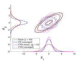
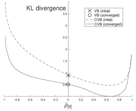
Figure 11: CVB and VB approximations $\widetilde{f}_{\boldsymbol{\theta}}$ for a zero-mean bivariate Gaussian distribution $f_{\boldsymbol{\theta}}$, with true variances $\sigma_{1}^{2}=4$, $\sigma_{2}^{2}=1$ and correlation coefficient $\rho=0.8$. The initial guess values for CVB and VB are $\widetilde{\sigma}_{1}^{[0]}=\widetilde{\sigma}_{2}^{[0]}=1$, together with various $\widetilde{\rho}_{[0]}\in(-1,1)$ for CVB. The cases $\widetilde{\rho}_{[0]}=0.5$ and $\widetilde{\rho}_{[0]}=-0.5$ are shown on the left and middle panel, respectively. The marginal distributions, which are also Gaussian, are plotted on two axes in these two panels. The lower KL divergence $\text{KL}(\widetilde{f}_{\boldsymbol{\theta}}||f_{\boldsymbol{\theta}})$ on the right panel, the better approximation, as illustrated in Fig. 7, 9. The CVB will be exact, i.e. $\text{KL}(\widetilde{f}_{\boldsymbol{\theta}}||f_{\boldsymbol{\theta}})\approx 0$ at convergence, if the initial guess values $\widetilde{\rho}_{[0]}$ are in range $\widetilde{\rho}_{[0]}\in[0.6,0.7]$, which is close to the true value $\rho=0.8$. If $\widetilde{\rho}_{[0]}=0$, the CVB is equivalent to VB approximation in independent class. The number $\nu_{c}$ of iterations until convergence for VB and CVB are, respectively, 8 and $11.1\pm 5.2$, averaged over all cases of $\widetilde{\rho}_{[0]}\in(-1,1)$ for CVB. Only one marginal is updated per iteration.

VI-A Bivariate Gaussian distribution

In this subsection, let us approximate a bivariate Gaussian distribution $f(\boldsymbol{\theta})=\mathcal{N}_{\boldsymbol{\theta}}(0,\boldsymbol{\Sigma})$ with zero mean and covariance matrix $\boldsymbol{\Sigma}\triangleq\left[\begin{array}[]{cc}\sigma_{1}^{2}&\rho\sigma_{1}\sigma_{2}\\ \rho\sigma_{1}\sigma_{2}&\sigma_{2}^{2}\end{array}\right]$. The purpose is then to illustrate the performance of CVB and VB approximations for $f(\boldsymbol{\theta})$ with different values of correlation coefficient $\rho\in[-1,1]$.

For simple notation, let us denote the marginal and conditional distributions of $f(\boldsymbol{\theta})$ by $f_{1}=\mathcal{N}_{\theta_{1}}(0,\sigma_{1})$ and $f_{2|1}=\mathcal{N}_{\theta_{2}}(\beta_{2|1}\theta_{1},\sigma_{2|1})$, respectively, in which $\beta_{2|1}\triangleq\rho\frac{\sigma_{2}}{\sigma_{1}}$ and $\sigma_{2|1}\triangleq\sigma_{2}\sqrt{1-\rho^{2}}$.

VI-A1 CVB approximation

Since Gaussian distribution belongs to CEF class (26), the CVB form $\widetilde{f}_{\text{CVB}}^{[1]}=\widetilde{f}_{2|1}^{[0]}\widetilde{f}_{1}^{[1]}=\widetilde{f}_{1|2}^{[1]}\widetilde{f}_{2}^{[1]}$ in (25) is also Gaussian, as shown in (28). Then, given initial values $\tilde{\beta}_{2|1}^{[0]}\triangleq\widetilde{\rho}_{[0]}\frac{\widetilde{\sigma}_{2}^{[0]}}{\widetilde{\sigma}_{1}^{[0]}}$ and $\widetilde{\sigma}_{2|1}^{[0]}\triangleq\widetilde{\sigma}_{2}^{[0]}\sqrt{1-\widetilde{\rho}_{[0]}^{2}}$, we have $\widetilde{f}_{2|1}^{[0]}=\mathcal{N}_{\theta_{2}}(\tilde{\beta}_{2|1}^{[0]}\theta_{1},\widetilde{\sigma}_{2|1}^{[0]})$. At iteration $\nu=1$, the CVA form (23) yields:

$$\widetilde{f}_{1}^{[1]} =\frac{1}{\zeta_{1}^{[1]}}\frac{f_{1}}{\exp(\text{KL}_{\widetilde{f}_{2|1}^{[0]}||f_{2|1}})}$$

$$=\frac{1}{\zeta_{1}^{[1]}}\frac{\frac{1}{\sigma_{1}\sqrt{2\pi}}\exp-\frac{\theta_{1}^{2}}{2\sigma_{1}^{2}}}{\frac{\sigma_{2|1}}{\widetilde{\sigma}_{2|1}^{[0]}}\exp\frac{1}{2}\left[\frac{\left(\tilde{\beta}_{2|1}^{[0]}-\beta_{2|1}\right)^{2}\theta_{1}^{2}+(\widetilde{\sigma}_{2|1}^{[0]})^{2}}{\sigma_{2|1}^{2}}-1\right]}$$

$$=\mathcal{N}_{\theta_{1}}(0,\widetilde{\sigma}_{1}^{[1]}),$$

in which $\text{KL}_{\widetilde{f}_{2|1}^{[0]}||f_{2|1}}$ is KL divergence between Gaussian distributions and:

$$\widetilde{\sigma}_{1}^{[1]} =\frac{1}{\sqrt{\frac{1}{\sigma_{1}^{2}}+\frac{\left(\tilde{\beta}_{2|1}^{[0]}-\beta_{2|1}\right)^{2}}{\sigma_{2}^{2}(1-\rho^{2})}}},\ \zeta_{1}^{[1]}=\frac{\widetilde{\sigma}_{1}^{[1]}}{\sigma_{1}}\frac{\widetilde{\sigma}_{2|1}^{[0]}}{\sigma_{2|1}}\exp\frac{\sigma_{2|1}^{2}-(\widetilde{\sigma}_{2|1}^{[0]})^{2}}{2\sigma_{2|1}^{2}}.$$ (42)

Then, in order to derive the reverse form $\widetilde{f}_{1|2}^{[1]}\widetilde{f}_{2}^{[1]}=\widetilde{f}_{2|1}^{[0]}\widetilde{f}_{1}^{[1]}$, let us firstly note that $\tilde{\beta}_{2|1}^{[0]}=\tilde{\beta}_{2|1}^{[1]}$ and $\widetilde{\sigma}_{2|1}^{[0]}=\widetilde{\sigma}_{2|1}^{[1]}$ , since the conditional form $\widetilde{f}_{2|1}$ of two distributions $\widetilde{f}_{2|1}^{[0]}\widetilde{f}_{1}^{[0]}$ and $\widetilde{f}_{2|1}^{[0]}\widetilde{f}_{1}^{[1]}=\widetilde{f}_{1|2}^{[1]}\widetilde{f}_{2}^{[1]}$ are still the same. Then, the updated parameters are:

$$\begin{cases}\tilde{\beta}_{2|1}^{[0]}&=\tilde{\beta}_{2|1}^{[1]}\\ \widetilde{\sigma}_{2|1}^{[0]}&=\widetilde{\sigma}_{2|1}^{[1]}\end{cases}\Leftrightarrow\begin{cases}\widetilde{\rho}_{[0]}\frac{\widetilde{\sigma}_{2}^{[0]}}{\widetilde{\sigma}_{1}^{[0]}}&=\widetilde{\rho}_{[1]}\frac{\widetilde{\sigma}_{2}^{[1]}}{\widetilde{\sigma}_{1}^{[1]}}\\ \widetilde{\sigma}_{2}^{[0]}\sqrt{1-\widetilde{\rho}_{[0]}^{2})}&=\widetilde{\sigma}_{2}^{[1]}\sqrt{1-\widetilde{\rho}_{[1]}^{2}}\end{cases}$$

which, by solving for $\widetilde{\rho}_{[1]}$ and $\widetilde{\sigma}_{2}^{[1]}$, yields:

$$\widetilde{\rho}_{[1]}^{2} =\frac{\widetilde{\rho}_{[0]}^{2}}{\widetilde{\rho}_{[0]}^{2}+\left(\frac{\widetilde{\sigma}_{1}^{[0]}}{\widetilde{\sigma}_{1}^{[1]}}\right)^{2}(1-\widetilde{\rho}_{[0]}^{2})},$$

$$\widetilde{\sigma}_{2}^{[1]} =\widetilde{\sigma}_{2}^{[0]}\sqrt{\widetilde{\rho}_{[0]}^{2}\left(\frac{\widetilde{\sigma}_{1}^{[1]}}{\widetilde{\sigma}_{1}^{[0]}}\right)^{2}+(1-\widetilde{\rho}_{[0]}^{2}))}.$$

Hence, we have $\tilde{\beta}_{1|2}^{[1]}=\widetilde{\rho}_{[1]}\frac{\widetilde{\sigma}_{1}^{[1]}}{\widetilde{\sigma}_{2}^{[1]}}$ and $\widetilde{\sigma}_{1|2}^{[1]}=\widetilde{\sigma}_{1}^{[1]}\sqrt{1-\widetilde{\rho}_{[1]}^{2}}$, which yield the updated forms $\widetilde{f}_{2}^{[1]}=\mathcal{N}_{\theta_{1}}(0,\widetilde{\sigma}_{2}^{[1]})$ and $\widetilde{f}_{1|2}^{[1]}=\mathcal{N}_{\theta_{1}}(\tilde{\beta}_{1|2}^{[1]}\theta_{2},\widetilde{\sigma}_{1|2}^{[1]})$. Reversing the role of $\theta_{1}$ with $\theta_{2}$ and repeating the above steps for iteration $\nu>1$, we will achieve the CVB approximation at convergence $\nu=\nu_{c}$, with $\text{KL}_{\widetilde{f}_{\text{CVB}}^{[\nu]}||f}=\log\frac{1}{\zeta_{1}^{[\nu]}}$.

The CVB approximation will be exact if its conditional mean and variance are exact, i.e. $\tilde{\beta}_{2|1}^{[\nu_{c}]}=\beta_{2|1}$ and $\widetilde{\sigma}_{2|1}^{[\nu_{c}]}=\sigma_{2|1}$, since we have $\text{KL}_{\widetilde{f}_{\text{CVB}}^{[\nu_{c}]}||f}=\log\frac{1}{\zeta_{1}^{[\nu_{c}]}}=0$ in this case, as shown in (42).

VI-A2 VB approximation

Since VB is a special case of CVB in independence space, we can simply set $\rho=0$ in above CVB algorithm and the result will be VB approximation.

VI-A3 Simulation’s results

The CVB and VB approximations for the case of $f(\boldsymbol{\theta})=\mathcal{N}_{\boldsymbol{\theta}}(0,\boldsymbol{\Sigma})$ are illustrated in Fig. 11. Since $\text{KL}_{\widetilde{f}_{\boldsymbol{\theta}}^{[\nu]}||f_{\boldsymbol{\theta}}}$ monotonically decreases with iteration $\nu$, the right panel shows the value of KL divergence at initialization $\nu=0$ and at convergence $\nu=\nu_{c}$, with $0\leq\text{KL}(\widetilde{f}_{\boldsymbol{\theta}}^{[\nu_{c}-1]}||f_{\boldsymbol{\theta}})-\text{KL}(\widetilde{f}_{\boldsymbol{\theta}}^{[\nu_{c}]}||f_{\boldsymbol{\theta}})\leq 0.01$. We can see that VB is a mean-field approximation and, hence, cannot accurately approximate a correlated Gaussian distribution. In contrast, the CVB belongs to a conditional copula class and, hence, can yield higher accuracy. In this sense, CVB can potentially return a globally optimal approximation for a correlated distribution, while VB can only return a locally optimal approximation.

Nevertheless, since the iterative CVB cannot escape its initialized copula class, its accuracy depends heavily on initialization. A solution for this issue is to initialize CVB with some information of original distribution. For example, merely setting the initial sign of $\widetilde{\rho}_{[0]}$ equal to the sign of true value $\rho$ would gain tremendously higher accuracy for CVB at convergence, as shown in the left and middle panel of Fig. 11.

Another solution for CVB’s initialization issue is to generate a lot of potential structures initially and take the average of the results at convergence. This CVB’s mixture-scheme will be illustrated in the next subsection.

VI-B Gaussian mixture clustering

  

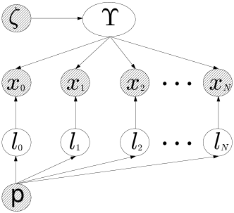
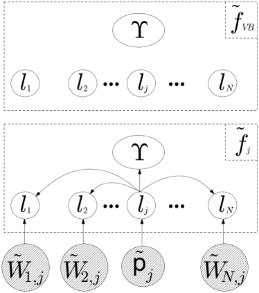
Figure 12: Directed acyclic graphs (DAG) for Gaussian clustering model with uniform hyper-parameters $\zeta$, $\boldsymbol{p}$ (left), the VB approximation with independent structure (upper right) and the CVB approximations (lower right). All variables in shaded nodes are known, while the others are random variables. Each $\widetilde{f}_{j}$ is a ternary structure centered around $l_{j}$, $j\in\{1,2,\ldots,N\}$. The augmented CVB approximation $\widetilde{f}_{0}=\sum_{j=1}^{N}q_{j}^{*}\widetilde{f}_{j}$ is designed in (70) and illustrated in Fig. 10.

In this subsection, let us illustrate the performance of CVB for a simple bivariate Gaussian mixture model. For this purpose, let us consider clusters of bivariate observation data $\boldsymbol{X}\triangleq[\boldsymbol{x}{}_{1},\boldsymbol{x}{}_{2},\ldots,\boldsymbol{x}_{N}]\in\mathbb{R}^{2\times N}$, such that $\boldsymbol{x}_{i}=[x_{1,i},x_{2,i}]^{T}\in\mathbb{R}^{2}$ at each time $i\in\{1,2,\ldots,N\}$ randomly belongs to one of $K$ bivariate independent Gaussian clusters $\mathcal{N}_{\boldsymbol{x}_{i}}(\boldsymbol{\mu},\mathbf{I}_{2})$ with equal probability $\boldsymbol{p}\triangleq[p{}_{1},p{}_{2},\ldots,p_{K}]^{T}$, i.e. $p_{k}=\frac{1}{K}$, $\forall k\in\{1,2,\ldots,K\}$, at unknown means $\boldsymbol{\Upsilon}\triangleq[\boldsymbol{\mu}{}_{1},\boldsymbol{\mu}{}_{2},\ldots,\boldsymbol{\mu}_{K}]\in\mathbb{R}^{2\times K}$. $\mathbf{I}_{2}$ denotes the $2\times 2$ identity covariance matrix.

Let us also define a temporal matrix $\boldsymbol{L}\triangleq[\boldsymbol{l}{}_{1},\boldsymbol{l}{}_{2},\ldots,\boldsymbol{l}_{N}]\in\mathbb{I}^{K\times N}$ of categorical vector labels $\boldsymbol{l}_{i}=[l{}_{1,i},l{}_{2,i},\ldots,l_{K,i}]^{T}\in\{\boldsymbol{\epsilon}{}_{1},\boldsymbol{\epsilon}{}_{2},\ldots,\boldsymbol{\epsilon}_{K}\}$, where $\boldsymbol{\epsilon}_{k}=[0,\ldots,1,\ldots 0]^{T}\in\mathbb{I}^{K}$ denotes the boolean vector with $k$-th non-zero element. By this way, we set $\boldsymbol{l}_{i}=\boldsymbol{\epsilon}_{k}$ if $\boldsymbol{x}_{i}$ belongs to $k$-th cluster. Then, by probability chain rule, our model is a Gaussian mixture $f(\boldsymbol{X},\boldsymbol{\Theta})=f(\boldsymbol{X}|\boldsymbol{\Theta})f(\boldsymbol{\Theta})$, in which $\boldsymbol{\Theta}\triangleq[\boldsymbol{\Upsilon},\boldsymbol{L}]$ are unknown parameters, as follows:

$$f(\boldsymbol{X},\boldsymbol{\Upsilon},\boldsymbol{L}) =f(\boldsymbol{X}|\boldsymbol{\Upsilon},\boldsymbol{L})f(\boldsymbol{\Upsilon},\boldsymbol{L})$$

$$=f(\boldsymbol{\Upsilon}|\boldsymbol{L},\boldsymbol{X})f(\boldsymbol{L},\boldsymbol{X})$$ (43)

$$=f(\boldsymbol{L}|\boldsymbol{\Upsilon},\boldsymbol{X})f(\boldsymbol{\Upsilon},\boldsymbol{X}).$$

In the first line of (43), the distributions are:

$$f(\boldsymbol{X}|\boldsymbol{\Upsilon},\boldsymbol{L}) =\prod_{i=1}^{N}f(\boldsymbol{x}_{i}|\boldsymbol{\Upsilon},\boldsymbol{l}_{i})=\prod_{i=1}^{N}\prod_{k=1}^{K}\mathcal{N}_{\boldsymbol{x}_{i}}^{l_{k,i}}(\boldsymbol{\mu}_{k},\mathbf{I}_{2}),$$

$$f(\boldsymbol{\Upsilon},\boldsymbol{L}) =f(\boldsymbol{\Upsilon})f(\boldsymbol{L})=\frac{1}{\zeta K^{N}},$$ (44)

in which the prior $f(\boldsymbol{L})=\prod_{i=1}^{N}\boldsymbol{l}_{i}^{T}\boldsymbol{p}=\frac{1}{K^{N}}$ is uniform by default and $f(\boldsymbol{\Upsilon})$ is the non-informative prior over $\mathbb{R}^{2\times K}$, i.e. $f(\boldsymbol{\Upsilon})=\frac{1}{\zeta}$, with constant $\zeta$ being set as high as possible (ideally $\zeta\rightarrow\infty$).

The second line of (43) can be written as follows:

$$f(\boldsymbol{\Upsilon}|\boldsymbol{L},\boldsymbol{X}) =\prod_{k=1}^{K}\mathcal{N}_{\boldsymbol{\mu}_{k}}\left(\overline{\boldsymbol{\mu}}_{k}(\boldsymbol{L}),\overline{\sigma}_{k}(\boldsymbol{L})\mathbf{I}_{2}\right),$$ (45)

$$f(\boldsymbol{L},\boldsymbol{X}) =\frac{1}{\zeta K^{N}}\prod_{k=1}^{K}\gamma_{k}(\boldsymbol{L}),$$

with $\overline{\boldsymbol{\mu}}_{k}(\boldsymbol{L})$ and $\overline{\sigma}_{k}(\boldsymbol{L})$ denoting posterior mean and standard deviation of $\boldsymbol{\mu}_{k}$, respectively, and $\gamma_{k}(\boldsymbol{L})$ denoting the updated form of weight’s probability $p_{k}=\frac{1}{K}$, as follows:

$$\overline{\boldsymbol{\mu}}_{k}(\boldsymbol{L}) \triangleq\frac{\sum_{i=1}^{N}l_{k,i}\boldsymbol{x}_{i}}{\sum_{i=1}^{N}l_{k,i}},\ \overline{\sigma}_{k}(\boldsymbol{L})\triangleq\frac{1}{\sqrt{\sum_{i=1}^{N}l_{k,i}}},$$ (46)

$$\gamma_{k}(\boldsymbol{L}) \triangleq 2\pi\overline{\sigma}_{k}^{2}(\boldsymbol{L})\prod_{i=1}^{N}\mathcal{N}_{\boldsymbol{x}_{i}}^{l_{k,i}}(\overline{\boldsymbol{\mu}}_{k}(\boldsymbol{L}),\mathbf{I}_{2}),$$

Note that, the first form (44) is equivalent to the second form (45-46) since we have:

$$\frac{\sum_{i=1}^{N}l_{k,i}||\boldsymbol{x}_{i}-\boldsymbol{\mu}_{k}||^{2}}{\sum_{i=1}^{N}l_{k,i}} =\frac{\sum_{i=1}^{N}l_{k,i}||\boldsymbol{x}_{i}-\overline{\boldsymbol{\mu}}_{k}(\boldsymbol{L})||^{2}}{\sum_{i=1}^{N}l_{k,i}}$$

$$+||\boldsymbol{\mu}_{k}-\overline{\boldsymbol{\mu}}_{k}(\boldsymbol{L})||^{2},$$ (47)

owing to Bregman variance theorem in (6), (13).

Similarly, the third line in (43) can be derived from (44), as follows:

$$f(\boldsymbol{X},\boldsymbol{\Upsilon})=\sum_{\boldsymbol{L}} f(\boldsymbol{X},\boldsymbol{\Upsilon},\boldsymbol{L})=\frac{\prod_{i=1}^{N}\sum_{k=1}^{K}\mathcal{N}_{\boldsymbol{x}_{i}}(\boldsymbol{\mu}_{k},\mathbf{I}_{2})}{\zeta K^{N}},$$

$$f(\boldsymbol{L}|\boldsymbol{\Upsilon},\boldsymbol{X})= \frac{f(\boldsymbol{X},\boldsymbol{\Upsilon},\boldsymbol{L})}{f(\boldsymbol{\Upsilon},\boldsymbol{X})}=\prod_{i=1}^{N}\underset{f(\boldsymbol{l}_{i}|\boldsymbol{\Upsilon},\boldsymbol{x}_{i})}{\underbrace{\frac{\prod_{k=1}^{K}\mathcal{N}_{\boldsymbol{x}_{i}}^{l_{k,i}}(\boldsymbol{\mu}_{k},\mathbf{I}_{2})}{\sum_{k=1}^{K}\mathcal{N}_{\boldsymbol{x}_{i}}(\boldsymbol{\mu}_{k},\mathbf{I}_{2})}}}.$$ (48)

Note that, the model without labels $f(\boldsymbol{X},\boldsymbol{\Upsilon})=f(\boldsymbol{X}|\boldsymbol{\Upsilon})f(\boldsymbol{\Upsilon})$ in (48) is a mixture of $K^{N}$ Gaussian components with unknown means $\boldsymbol{\Upsilon}$, since we have augmented the model $f(\boldsymbol{X}|\boldsymbol{\Upsilon})$ with label’s form $f(\boldsymbol{X}|\boldsymbol{\Upsilon},\boldsymbol{L})$ above. The posterior form $f(\boldsymbol{\Upsilon}|\boldsymbol{X})\propto f(\boldsymbol{X},\boldsymbol{\Upsilon})=\sum_{\boldsymbol{L}}f(\boldsymbol{X},\boldsymbol{\Upsilon},\boldsymbol{L})$ in this case is intractable, since its normalization’s complexity $\mathcal{O}(K^{N})$ grows exponentially with number of data $N$, hence the curse of dimensionality.

VI-B1 ICM and k-means algorithms

From (45-46), we can see that the conditional mean $\overline{\boldsymbol{\mu}}_{k}(\boldsymbol{L})$ is actually the $k$-th clustering sample’s mean of $\boldsymbol{\mu}_{k}$, given all possible boolean values of $l_{k,i}\in\mathbb{I}=\{0,1\}$ over time $i\in\{1,2,\ldots,N\}.$ The probability of categorical label $f(\boldsymbol{L}|\boldsymbol{X})\propto f(\boldsymbol{L},\boldsymbol{X})$ in (45) is, in turn, calculated as the distance of all observation $\boldsymbol{x}_{i}$ to sample’s mean $\overline{\boldsymbol{\mu}}_{k}$ of each cluster $k\in\{1,2,\ldots,K\}$ via $\gamma_{k}(\boldsymbol{L})$ in (46). Nevertheless, since the weights $\gamma_{k}(\boldsymbol{L})$ in (45-46) are not factorable over $\boldsymbol{L}$, the posterior probability $f(\boldsymbol{L}|\boldsymbol{X})$ needs to be computed brute-forcedly over all $K^{N}$ possible values of label matrix $\boldsymbol{L}$ as a whole and, hence, yields the curse of dimensionality.

A popular solution for this case is the k-means algorithm, which is merely an application of iteratively conditional mode (ICM) algorithm (31) to above clustering mixture (45), (48), as follows:

$$\widehat{\boldsymbol{\Upsilon}}^{[\nu]} =\operatornamewithlimits{arg\,max}_{\boldsymbol{\Upsilon}}f(\boldsymbol{\Upsilon}|\widehat{\boldsymbol{L}}^{[\nu-1]},\boldsymbol{X}),$$ (49)

$$\widehat{\boldsymbol{L}}^{[\nu]} =\operatornamewithlimits{arg\,max}_{\boldsymbol{L}}f(\boldsymbol{L}|\widehat{\boldsymbol{\mu}}^{[\nu]},\boldsymbol{X}).$$

where $\widehat{\boldsymbol{\Upsilon}}^{[\nu]}\triangleq[\widehat{\boldsymbol{\mu}}{}_{1}^{[\nu]},\widehat{\boldsymbol{\mu}}{}_{2}^{[\nu]},\ldots,\widehat{\boldsymbol{\mu}}_{K}^{[\nu]}]$ and $\widehat{\boldsymbol{L}}^{[\nu]}\triangleq[\widehat{\boldsymbol{l}}{}_{1}^{[\nu]},\widehat{\boldsymbol{l}}{}_{2}^{[\nu]},\ldots,\widehat{\boldsymbol{l}}_{N}^{[\nu]}]$. Since the mode of Gaussian distribution is also its mean value, let us substitute (49) to $f(\boldsymbol{\Upsilon}|\boldsymbol{L},\boldsymbol{X})$ in (45-46) and $f(\boldsymbol{L}|\boldsymbol{\Upsilon},\boldsymbol{X})$ in (48), as follows:

$$\widehat{\boldsymbol{\mu}}_{k}^{[\nu]} =\overline{\boldsymbol{\mu}}_{k}(\widehat{\boldsymbol{L}}^{[\nu-1]})=\frac{\sum_{i=1}^{N}\widehat{l}_{k,i}^{[\nu-1]}\boldsymbol{x}_{i}}{\sum_{i=1}^{N}\widehat{l}_{k,i}^{[\nu-1]}},$$

$$\widehat{k}_{i}^{[\nu]} =\operatornamewithlimits{arg\,max}_{k}\mathcal{N}_{\boldsymbol{x}_{i}}(\overline{\boldsymbol{\mu}}_{k}^{[\nu]},\mathbf{I}_{2})$$ (50)

$$=\operatornamewithlimits{arg\,min}_{k}||\boldsymbol{x}_{i}-\overline{\boldsymbol{\mu}}_{k}^{[\nu]}||^{2},$$

in which the form of $\overline{\boldsymbol{\mu}}_{k}$ is given in (46), $\widehat{\boldsymbol{l}}_{i}^{[\nu]}\triangleq[\widehat{l}{}_{1,i}^{[\nu]},\widehat{l}{}_{2,i}^{[\nu]},\ldots,\widehat{l}_{K,i}^{[\nu]}]^{T}$ and $\widehat{l}_{k,i}^{[\nu]}=\delta[k-\widehat{k}_{i}^{[\nu]}]$, with $\delta[\cdot]$ denoting the Kronecker delta function, $\forall i\in\{1,2,\ldots,N\}$. By convention, we keep $\widehat{\boldsymbol{\mu}}_{k}^{[\nu]}=\widehat{\boldsymbol{\mu}}_{k}^{[\nu-1]}$ unchanged if $\sum_{i=1}^{N}\widehat{l}_{k,i}^{[\nu-1]}=0$, since no update for $k$-th cluster is found in this case.

From (50), we can see that the algorithm starts with $K$ initial mean values $\overline{\boldsymbol{\mu}}_{k}^{[0]}$, $\forall k\in\{1,2,\ldots,K\}$, then assigns categorical labels to clusters via minimum Euclidean distance in (50), which, in turn, yields $K$ new cluster’s means $\overline{\boldsymbol{\mu}}_{k}^{[1]}$, $\forall k\in\{1,2,\ldots,K\}$, and so forth. Hence it is called the k-means algorithm in literature [25, 26].

At convergence $\nu=\nu_{c}$, the k-means algorithm returns a locally joint MAP value $\widehat{\boldsymbol{\Theta}}^{[\nu_{c}]}=\text{[$\widehat{\boldsymbol{\Upsilon}}^{[\nu_{c}]}$,$\widehat{\boldsymbol{L}}^{[\nu_{c}]}$]}$, which depends on initial guess value $\widehat{\boldsymbol{\Theta}}^{[0]}$.

From Corollary 34, the convergence of ELBO can be used as a stopping rule, as follows:

$$\text{ELBO}_{\text{ICM}}^{[\nu]} =\log f(\boldsymbol{X},\widehat{\boldsymbol{\Upsilon}}^{[\nu]},\widehat{\boldsymbol{L}}^{[\nu]})$$

$$=\log\frac{\prod_{i=1}^{N}\prod_{k=1}^{K}\mathcal{N}_{\boldsymbol{x}_{i}}^{\widehat{l}_{k,i}^{[\nu]}}(\widehat{\boldsymbol{\mu}}_{k}^{[\nu]},\mathbf{I}_{2})}{\zeta K^{N}},$$

since $\text{KL}_{\widetilde{f}_{\text{ICM}}^{[\nu]}||f}=-\text{ELBO}_{\text{ICM}}^{[\nu]}+\log f(\boldsymbol{X}),$ as shown in (34).

VI-B2 EM algorithms

Let us now derive two EM approximations for true posterior distribution $f(\boldsymbol{\Upsilon},\boldsymbol{L}|\boldsymbol{X})$ via (30), as follows:

$$\widetilde{f}_{\text{EM}_{1}}(\boldsymbol{\Upsilon},\boldsymbol{L}|\boldsymbol{X}) =f(\boldsymbol{\Upsilon}|\widehat{\boldsymbol{L}}_{\text{EM}_{1}},\boldsymbol{X})\delta[\boldsymbol{L}-\widehat{\boldsymbol{L}}_{\text{EM}_{1}}],$$

$$\widetilde{f}_{\text{EM}_{2}}(\boldsymbol{\Upsilon},\boldsymbol{L}|\boldsymbol{X}) =f(\boldsymbol{L}|\widehat{\boldsymbol{\Upsilon}}_{\text{EM}_{2}},\boldsymbol{X})\delta(\boldsymbol{\Upsilon}-\widehat{\boldsymbol{\Upsilon}}_{\text{EM}_{2}}).$$ (51)

Since our joint model $f(\boldsymbol{\Upsilon},\boldsymbol{L},\boldsymbol{X})$ in (43-48) is of CEF form (26), the EM forms (51) can be feasibly identified via (28), as follows:

$$\widehat{\boldsymbol{L}}_{\text{EM}_{1}}^{[\nu]} =\operatornamewithlimits{arg\,max}_{\boldsymbol{L}}\mathbb{E}_{f(\boldsymbol{\Upsilon}|\widehat{\boldsymbol{L}}_{\text{EM}_{1}}^{[\nu-1]},\boldsymbol{X})}\log f(\boldsymbol{X},\boldsymbol{\Upsilon},\boldsymbol{L}),$$ (52)

$$\widehat{\boldsymbol{\Upsilon}}_{\text{EM}_{2}}^{[\nu]} =\operatornamewithlimits{arg\,max}_{\boldsymbol{\Upsilon}}\mathbb{E}_{f(\boldsymbol{L}|\widehat{\boldsymbol{\Upsilon}}_{\text{EM}_{2}}^{[\nu-1]},\boldsymbol{X})}\log f(\boldsymbol{X},\boldsymbol{\Upsilon},\boldsymbol{L}),$$ (53)

where $f(\boldsymbol{\Upsilon}|\widehat{\boldsymbol{L}}_{\text{EM}_{1}}^{[\nu-1]},\boldsymbol{X})=\prod_{k=1}^{K}\mathcal{N}_{\boldsymbol{\mu}_{k}}(\widetilde{\boldsymbol{\mu}}_{k}^{[\nu]},\widetilde{\sigma}_{k}^{[\nu]}\mathbf{I}_{2})$ and $f(\boldsymbol{L}|\widehat{\boldsymbol{\Upsilon}}_{\text{EM}_{2}}^{[\nu-1]},\boldsymbol{X})=\prod_{i=1}^{N}Mu_{\boldsymbol{l}_{i}}(\widetilde{\boldsymbol{p}}_{i}^{[\nu-1]})$.

Replacing $\boldsymbol{\Upsilon}$ and $\boldsymbol{L}$ in $f(\boldsymbol{X},\boldsymbol{\Upsilon},\boldsymbol{L})$ in (52) and (53) with $\widetilde{\boldsymbol{\Upsilon}}^{[\nu-1]}\triangleq\mathbb{E}_{f(\boldsymbol{\Upsilon}|\widehat{\boldsymbol{L}}_{\text{EM}_{1}}^{[\nu-1]},\boldsymbol{X})}(\boldsymbol{\Upsilon})$ and $\widetilde{\boldsymbol{P}}^{[\nu-1]}\triangleq\mathbb{E}_{f(\boldsymbol{L}|\widehat{\boldsymbol{\Upsilon}}_{\text{EM}_{2}}^{[\nu-1]},\boldsymbol{X})}(\boldsymbol{L})$, we then have, respectively:

$$\widetilde{\boldsymbol{\mu}}_{k}^{[\nu]} =\overline{\boldsymbol{\mu}}_{k}(\widehat{\boldsymbol{L}}_{\text{EM}_{1}}^{[\nu-1]}),\ \widetilde{\sigma}_{k}^{[\nu]}=\overline{\sigma}_{k}(\widehat{\boldsymbol{L}}_{\text{EM}_{1}}^{[\nu-1]}),$$

$$\widehat{k}_{i}^{[\nu]} =\operatornamewithlimits{arg\,max}_{k}\frac{\mathcal{N}_{\boldsymbol{x}_{i}}(\widetilde{\boldsymbol{\mu}}_{k}^{[\nu]},\mathbf{I}_{2})}{\exp((\widetilde{\sigma}_{k}^{[\nu]})^{2})},$$ (54)

and:

$$\widetilde{p}_{k,i}^{[\nu]} \propto\mathcal{N}_{\boldsymbol{x}_{i}}(\widehat{\boldsymbol{\mu}}_{k}^{[\nu]},\mathbf{I}_{2}),$$ (55)

$$\widehat{\boldsymbol{\mu}}_{k}^{[\nu]} =\overline{\boldsymbol{\mu}}_{k}(\widetilde{\boldsymbol{P}}^{[\nu-1]})=\frac{\sum_{i=1}^{N}\widetilde{p}_{k,i}^{[\nu-1]}\boldsymbol{x}_{i}}{\sum_{i=1}^{N}\widetilde{p}_{k,i}^{[\nu-1]}},$$

where $\widehat{\boldsymbol{\Upsilon}}_{\text{EM}_{2}}^{[\nu]}\triangleq[\widehat{\boldsymbol{\mu}}{}_{1}^{[\nu]},\widehat{\boldsymbol{\mu}}{}_{2}^{[\nu]},\ldots,\widehat{\boldsymbol{\mu}}_{K}^{[\nu]}]$, $\widetilde{\boldsymbol{\Upsilon}}^{[\nu]}\triangleq[\widetilde{\boldsymbol{\mu}}{}_{1}^{[\nu]},\widetilde{\boldsymbol{\mu}}{}_{2}^{[\nu]},\ldots,\widetilde{\boldsymbol{\mu}}_{K}^{[\nu]}]$, $\widehat{\boldsymbol{L}}_{\text{EM}_{1}}^{[\nu]}\triangleq[\widehat{\boldsymbol{l}}{}_{1}^{[\nu]},\widehat{\boldsymbol{l}}{}_{2}^{[\nu]},\ldots,\widehat{\boldsymbol{l}}_{N}^{[\nu]}]$ with $\widehat{\boldsymbol{l}}_{i}^{[\nu]}\triangleq[\widehat{l}{}_{1,i},\widehat{l}{}_{2,i},\ldots,\widehat{l}_{K,i}]^{T}$ and $\widehat{l}_{k,i}^{[\nu]}=\delta[k-\widehat{k}_{i}^{[\nu]}]$, $\widetilde{\boldsymbol{P}}^{[\nu]}\triangleq[\widetilde{\boldsymbol{p}}{}_{1}^{[\nu]},\widetilde{\boldsymbol{p}}{}_{2}^{[\nu]},\ldots,\widetilde{\boldsymbol{p}}_{N}^{[\nu]}]$ with $\sum_{k=1}^{K}\widetilde{p}_{k,i}^{[\nu]}=1$, $\forall i\in\{1,2,\ldots,N\}$.

The forms $\overline{\boldsymbol{\mu}}_{k}$ and $\overline{\sigma}_{k}$ are given in (46). By convention, we keep $\widetilde{\boldsymbol{\mu}}_{k}^{[\nu]}=\widetilde{\boldsymbol{\mu}}_{k}^{[\nu-1]}$ and $\widetilde{\sigma}_{k}^{[\nu]}=\widetilde{\sigma}_{k}^{[\nu-1]}$ unchanged if $\sum_{i=1}^{N}\widehat{l}_{k,i}^{[\nu-1]}=0$ in (54).

Also, since $f(\boldsymbol{\Upsilon},\boldsymbol{L},\boldsymbol{X})$ is of CEF form (26), we can feasibly evaluate $\text{KL}_{\widetilde{f}_{\text{EM}}^{[\nu]}||f(\boldsymbol{X},\boldsymbol{\Upsilon},\boldsymbol{L})}$ directly for $\widetilde{f}_{\text{EM}_{1}}^{[\nu]}$and $\widetilde{f}_{\text{EM}_{2}}^{[\nu]}$, as defined in (51). The convergence of $\text{ELBO}_{\text{EM}}^{[\nu]}$, as given in (33), is then computed as follows:

$$\text{ELBO}_{\text{EM}}^{[\nu]} =-\text{KL}_{\widetilde{f}_{\text{EM}}^{[\nu]}||f(\boldsymbol{X},\boldsymbol{\Upsilon},\boldsymbol{L})}=\log\frac{\zeta_{\text{EM}}^{[\nu]}}{\zeta K^{N}},$$

$$\zeta_{\text{EM}_{1}}^{[\nu]} =\frac{f(\boldsymbol{\Upsilon}=\widetilde{\boldsymbol{\Upsilon}}^{[\nu]},\boldsymbol{L}=\widehat{\boldsymbol{L}}_{\text{EM}}^{[\nu]},\boldsymbol{X})}{\exp\left(\sum_{k=1}^{K}(\widetilde{\sigma}_{k}^{[\nu]})^{2}\sum_{i=1}^{N}\widehat{l}_{k,i}^{[\nu]}\right)}\prod_{k=1}^{K}((\widetilde{\sigma}_{k}^{[\nu]})^{2}2\pi e),$$

$$\zeta_{\text{EM}_{2}}^{[\nu]} =\frac{f(\boldsymbol{\Upsilon}=\widehat{\boldsymbol{\Upsilon}}_{\text{EM}}^{[\nu]},\boldsymbol{L}=\widetilde{\boldsymbol{P}}^{[\nu]},\boldsymbol{X})}{\prod_{k=1}^{K}\prod_{i=1}^{N}\widetilde{p}_{k,i}^{[\nu]\widetilde{p}_{k,i}^{[\nu]}}}.$$

Remark 40.

Comparing (54-55) with (50), we can see that the k-means algorithm only considers the mean (i.e. the first moment), while EM algorithm takes both mean and variance (i.e. the first and second moments) into account.

VI-B3 VB approximation

Let us now derive VB approximation $\widetilde{f}_{\text{VB}}(\boldsymbol{\Upsilon},\boldsymbol{L}|\boldsymbol{X})=\widetilde{f}_{\text{VB}}(\boldsymbol{\Upsilon}|\boldsymbol{X})\widetilde{f}_{\text{VB}}(\boldsymbol{L}|\boldsymbol{X})$ in (29) for true posterior distribution $f(\boldsymbol{\Upsilon},\boldsymbol{L}|\boldsymbol{X})$. Since $f(\boldsymbol{\Upsilon},\boldsymbol{L},\boldsymbol{X})$ is of CEF form (26), the VB form can be feasibly identified via (28), as follows:

$$\widetilde{f}_{\text{VB}}^{[\nu]}(\boldsymbol{\Upsilon}|\boldsymbol{X}) \propto\exp\mathbb{E}_{\widetilde{f}_{\text{VB}}^{[\nu-1]}(\boldsymbol{L}|\boldsymbol{X})}\log f(\boldsymbol{X},\boldsymbol{\Upsilon},\boldsymbol{L})$$ (56)

$$=\prod_{k=1}^{K}\mathcal{N}_{\boldsymbol{\mu}_{k}}\left(\widetilde{\boldsymbol{\mu}}_{k}^{[\nu]},\widetilde{\sigma}_{k}^{[\nu]}\mathbf{I}_{2}\right),$$

$$\widetilde{f}_{\text{VB}}^{[\nu]}(\boldsymbol{L}|\boldsymbol{X}) \propto\exp\mathbb{E}_{\widetilde{f}_{\text{VB}}^{[\nu]}(\boldsymbol{\Upsilon}|\boldsymbol{X})}\log f(\boldsymbol{X},\boldsymbol{\Upsilon},\boldsymbol{L})$$

$$=\prod_{i=1}^{N}\text{$Mu$}_{\boldsymbol{l}_{i}}\left(\widetilde{\boldsymbol{p}}_{i}^{[\nu]}\right),$$

Replacing $\boldsymbol{L}$ in (46) with $\widetilde{\boldsymbol{P}}^{[\nu]}=\mathbb{E}_{\widetilde{f}_{\text{VB}}^{[\nu]}(\boldsymbol{L}|\boldsymbol{X})}(\boldsymbol{L})$, we then have:

$$\widetilde{\boldsymbol{\mu}}_{k}^{[\nu]} =\overline{\boldsymbol{\mu}}_{k}(\widetilde{\boldsymbol{P}}^{[\nu-1]}),\ \widetilde{\sigma}_{k}^{[\nu]}=\overline{\sigma}_{k}(\widetilde{\boldsymbol{P}}^{[\nu-1]}),$$

$$\widetilde{p}_{k,i}^{[\nu]} \propto\frac{\mathcal{N}_{\boldsymbol{x}_{i}}(\widetilde{\boldsymbol{\mu}}_{k}^{[\nu]},\mathbf{I}_{2})}{\exp((\widetilde{\sigma}_{k}^{[\nu]})^{2})},$$ (57)

where $\widetilde{\boldsymbol{P}}^{[\nu]}\triangleq[\widetilde{\boldsymbol{p}}{}_{1}^{[\nu]},\widetilde{\boldsymbol{p}}{}_{2}^{[\nu]},\ldots,\widetilde{\boldsymbol{p}}_{N}^{[\nu]}]$ and $\sum_{k=1}^{K}\widetilde{p}_{k,i}^{[\nu]}=1$, $\forall i\in\{1,2,\ldots,N\}$. The forms $\overline{\boldsymbol{\mu}}_{k}$ and $\overline{\sigma}_{k}$ are given in (46).

From (56), let $\zeta_{\text{VB}}^{[\nu]}$ denote the normalizing constant of $\widetilde{f}_{\text{VB}}^{[\nu]}(\boldsymbol{\Upsilon}|\boldsymbol{X})=\frac{1}{\zeta_{\text{VB}}^{[\nu]}}\exp\mathbb{E}_{\widetilde{f}_{\text{VB}}^{[\nu-1]}(\boldsymbol{L}|\boldsymbol{X})}\log\frac{f(\boldsymbol{X},\boldsymbol{\Upsilon},\boldsymbol{L})}{\widetilde{f}_{\text{VB}}^{[\nu-1]}(\boldsymbol{L}|\boldsymbol{X})}$, similarly to (32). We then have:

$$\text{ELBO}_{\text{VB}}^{[\nu]}=\log\zeta_{\text{VB}}^{[\nu]}=\log\frac{1}{\zeta K^{N}}\prod_{k=1}^{K}\frac{\gamma_{k}(\widetilde{\boldsymbol{P}}^{[\nu]})}{\prod_{i=1}^{N}\widetilde{p}_{k,i}^{[\nu]\widetilde{p}_{k,i}^{[\nu]}}},$$ (58)

where $\gamma_{k}(\widetilde{\boldsymbol{P}}^{[\nu]})$ is given in (46), with $\boldsymbol{L}$ being replaced by $\widetilde{\boldsymbol{P}}^{[\nu]}$. The convergence of $\text{ELBO}_{\text{VB}}^{[\nu]}$, as mentioned in (33), can be used as a stopping rule.

Remark 41.

From (56-57), we can see that the VB algorithm combines two EM algorithms (51-55) together and takes all moments of clustering data into account.

VI-B4 CVB approximation

Let us now derive CVB approximation $\widetilde{f}_{\text{CVB}}^{[1]}=\widetilde{f}_{2|1}^{[0]}\widetilde{f}_{1}^{[1]}=\widetilde{f}_{1|2}^{[1]}\widetilde{f}_{2}^{[1]}$ for true posterior distribution $f(\boldsymbol{\Theta}|\boldsymbol{X})=f(\boldsymbol{\Upsilon},\boldsymbol{L}|\boldsymbol{X})$, with $\boldsymbol{\Theta}=[\boldsymbol{\Upsilon},\boldsymbol{L}]$, via (25), (32). Firstly, let us note that, the denominator $f(\boldsymbol{\Upsilon},\boldsymbol{X})$ of $f(\boldsymbol{L}|\boldsymbol{\Upsilon},\boldsymbol{X})$ in (48) is a mixture of $K^{N}$ Gaussian components, which is not factorable over its marginals on $\boldsymbol{\mu}_{k}$, $k\in\{1,2,\ldots,K\}$. Hence, a direct application of CVB algorithm (32) with $\boldsymbol{\theta}_{1}=\boldsymbol{L}$ and $\boldsymbol{\theta}_{2}=\boldsymbol{\Upsilon}$ would not yield a closed form for $\widetilde{f}_{CVB}(\boldsymbol{\Upsilon}|\boldsymbol{X})$, when the total number $K$ of clusters is not small.

• CVB’s ternary partition:

For a tractable form of $\widetilde{f}_{CVB}(\boldsymbol{\Upsilon}|\boldsymbol{X})$, let us now define two different binary partitions $\boldsymbol{\theta}_{1}$ and $\boldsymbol{\theta}_{2}$ for $\boldsymbol{\Theta}=[\boldsymbol{\Upsilon},\boldsymbol{L}]$ at each CVB’s iteration, as explained in subsection IV-B2:

$$f(\boldsymbol{\Theta}|\boldsymbol{X}) =\underset{f_{2|1}}{\underbrace{f(\boldsymbol{\Upsilon}|\boldsymbol{L},\boldsymbol{X})}}\underset{f_{1}}{\underbrace{f(\boldsymbol{L}|\boldsymbol{X})}}=\underset{f_{1|2}}{\underbrace{f(\boldsymbol{L}_{\backslash j}|\boldsymbol{\Upsilon},\boldsymbol{X})}}\underset{f_{2}}{\underbrace{f(\boldsymbol{\Upsilon},\boldsymbol{l}_{j}|\boldsymbol{X})},}$$

$$\widetilde{f}(\boldsymbol{\Theta}|\boldsymbol{X}) =\underset{\widetilde{f}_{2|1}}{\underbrace{\widetilde{f}(\boldsymbol{\Upsilon}|\boldsymbol{l}_{j},\boldsymbol{X})}}\underset{\widetilde{f}_{1}}{\underbrace{\widetilde{f}(\boldsymbol{L}|\boldsymbol{X})}}=\underset{\widetilde{f}_{1|2}}{\underbrace{\widetilde{f}(\boldsymbol{L}_{\backslash j}|\boldsymbol{l}_{j},\boldsymbol{X})}}\underset{\widetilde{f}_{2}}{\underbrace{\widetilde{f}(\boldsymbol{\Upsilon},\boldsymbol{l}_{j}|\boldsymbol{X})},}$$ (59)

for any node $j\in\{1,2,\ldots,N\}.$ Note that, the true conditional $f_{1|2}\triangleq f(\boldsymbol{L}_{\backslash j}|\boldsymbol{\Upsilon},\boldsymbol{l}_{j},\boldsymbol{X})=f(\boldsymbol{L}_{\backslash j}|\boldsymbol{\Upsilon},\boldsymbol{X})$ in (59) does not depends on $\boldsymbol{l}_{j}$, since $f(\boldsymbol{L}|\boldsymbol{\Upsilon},\boldsymbol{X})$ in (48) is conditionally independent, i.e. $f(\boldsymbol{L}|\boldsymbol{\Upsilon},\boldsymbol{X})=\prod_{i=1}^{N}f(\boldsymbol{l}_{i}|\boldsymbol{\Upsilon},\boldsymbol{X})$, as illustrated in Fig. 12.

Hence, given a ternary partition $\boldsymbol{\Theta}=[\boldsymbol{L}_{\backslash j},\boldsymbol{l}_{j},\boldsymbol{\Upsilon}]$ for each node $j$ in (59), we have set $\boldsymbol{\theta}_{1}=\boldsymbol{L}=[\boldsymbol{L}_{\backslash j},\boldsymbol{l}_{j}]$ and $\boldsymbol{\theta}_{2}=\boldsymbol{\Upsilon}$ in the forward form, but $\boldsymbol{\theta}_{1}=\boldsymbol{L}_{\backslash j}$ and $\boldsymbol{\theta}_{2}=[\boldsymbol{l}_{j},\boldsymbol{\Upsilon}]$ in reverse form in (59). The equality in CVB form $\widetilde{f}_{\text{CVB}}^{[1]}=\widetilde{f}_{2|1}^{[0]}\widetilde{f}_{1}^{[1]}=\widetilde{f}_{1|2}^{[1]}\widetilde{f}_{2}^{[1]}$ is still valid, since we still have the same joint parameters $\boldsymbol{\Theta}=[\boldsymbol{\Upsilon},\boldsymbol{L}]$ on both sides.

• CVB’s initialization:

Let us consider the left form in (59) first. For tractability, the initial CVB $\widetilde{f}_{2|1}^{[0]}\triangleq\widetilde{f}^{[0]}(\boldsymbol{\Upsilon}|\boldsymbol{l}_{j},\boldsymbol{X})$ will be set as a restricted form of the true conditional $f_{2|1}\triangleq f(\boldsymbol{\Upsilon}|\boldsymbol{L},\boldsymbol{X})$ in (45), as follows:

$$\widetilde{f}_{2|1}^{[0]}=\prod_{k=1}^{K}\widetilde{f}^{[0]}(\boldsymbol{\mu}_{k}|\boldsymbol{l}_{j})=\prod_{k=1}^{K}\prod_{m=1}^{K}\mathcal{N}_{\boldsymbol{\mu}_{k}}^{l_{m,j}}\left(\widetilde{\boldsymbol{\mu}}_{k,m,j}^{[0]},\widetilde{\sigma}_{k,m,j}^{[0]}\mathbf{I}_{2}\right)$$ (60)

where $\widetilde{\boldsymbol{\mu}}_{k,m,j}^{[0]}\in\mathbb{R}^{2}$ and $\widetilde{\sigma}_{k,m,j}^{[0]}>0$ are initial means and variances of $\widetilde{f}^{[0]}(\boldsymbol{\mu}_{k}|\boldsymbol{l}_{j})=\prod_{m=1}^{K}\widetilde{f}^{[0]}(\boldsymbol{\mu}_{k}|l_{m,j})$.

• CVB’s iteration (forward step):

Let us now apply CVB algorithm (32) to (59) and approximate $f_{1}\triangleq f(\boldsymbol{L}|\boldsymbol{X})$ via $\widetilde{f}_{2|1}^{[0]}$ in (60), as follows:

$$\widetilde{f}_{1}^{[1]}\triangleq \widetilde{f}^{[1]}(\boldsymbol{L}|\boldsymbol{X})=\frac{1}{\zeta_{1}^{[1]}}\exp\mathbb{E}_{\widetilde{f}_{2|1}^{[0]}}\log\frac{f(\boldsymbol{X},\boldsymbol{\Upsilon},\boldsymbol{L})}{\widetilde{f}_{2|1}^{[0]}}$$ (61)

$$=\frac{1}{\zeta_{1}^{[1]}\zeta K^{N}}\prod_{k=1}^{K}\prod_{m=1}^{K}(\widetilde{\kappa}_{k,m,j}^{[1]}\prod_{i=1}^{N}(\widetilde{\gamma}_{k,m,i,j}^{[1]})^{l_{k,i}})^{l_{m,j}},$$

in which $f(\boldsymbol{X},\boldsymbol{\Upsilon},\boldsymbol{L})$ is given in (43-44) and, hence:

$$\widetilde{\kappa}_{k,m,j}^{[1]}=2\pi e(\widetilde{\sigma}_{k,m,j}^{[0]})^{2},\ \widetilde{\gamma}_{k,m,i,j}^{[1]}\triangleq\frac{\mathcal{N}_{\boldsymbol{x}_{i}}(\widetilde{\boldsymbol{\mu}}_{k,m,j}^{[0]},\mathbf{I}_{2})}{\exp((\widetilde{\sigma}_{k,m,j}^{[0]})^{2})},$$ (62)

since we have $\exp\mathbb{E}_{\mathcal{N}_{\boldsymbol{\mu}}(\widetilde{\boldsymbol{\mu}},\widetilde{\sigma}\mathbf{I}_{2})}\log\frac{\mathcal{N}_{\boldsymbol{x}_{i}}(\boldsymbol{\mu},\mathbf{I}_{2})}{\mathcal{N}_{\boldsymbol{\mu}}(\widetilde{\boldsymbol{\mu}},\widetilde{\sigma}\mathbf{I}_{2})}=\frac{\mathcal{N}_{\boldsymbol{x}_{i}}(\widetilde{\boldsymbol{\mu}},\mathbf{I}_{2})\exp(-\widetilde{\sigma}^{2})}{1/(2\pi\widetilde{\sigma}^{2}e)}$ in general, as shown in (28). Comparing the true updated weights $\gamma_{k}(\boldsymbol{L})$ of $f_{1}$ in (46) with the approximated weights $\widetilde{\gamma}_{k,m,i,j}^{[1]}$ of $\widetilde{f}_{1}^{[1]}$ in (62), we can see that CVB algorithm has approximated the intractable forms $\{\overline{\boldsymbol{\mu}}_{k}(\boldsymbol{L}),\overline{\sigma}_{k}^{2}(\boldsymbol{L})\}$ with total $K^{N}$ elements by a factorized set of $N$ tractable forms $\{\widetilde{\boldsymbol{\mu}}_{k,m,j}^{[0]},\widetilde{\sigma}_{k,m,j}^{[0]}\}$ with only $K^{2}N$ elements.

Comparing (59) with (61), we can identify the form of $\widetilde{f}_{1|2}^{[1]}$ in (59), as follows:

$$\widetilde{f}_{1|2}^{[1]}\triangleq\widetilde{f}^{[1]}(\boldsymbol{L}_{\backslash j}|\boldsymbol{l}_{j},\boldsymbol{X}) =\prod_{i\neq j}\text{$Mu$}_{\boldsymbol{l}_{i}}\left(\widetilde{\boldsymbol{W}}_{i,j}^{[1]}\boldsymbol{l}_{j}\right)$$ (63)

where $\widetilde{\boldsymbol{W}}_{i,j}^{[1]}$ is a left stochastic matrix, whose $\{m,k\}$-element is the updated transition probability from $l_{m,j}$ to $l_{k,i}$: $\widetilde{w}_{k,m}^{[1]}(i,j)\triangleq\frac{\widetilde{\gamma}_{k,m,i,j}^{[1]}}{\sum_{k=1}^{K}\widetilde{\gamma}_{k,m,i,j}^{[1]}}$, $\forall i\neq j$. For later use, let us assign $\widetilde{\boldsymbol{W}}_{j,j}^{[\nu]}\triangleq\mathbf{I}_{K}$, with $\mathbf{I}_{K}$ denoting $K\times K$ identity matrix, when $i=j$, at any iteration $\nu$.

• CVB’s iteration (reverse step):

Let us apply CVB (32) to (59) again and approximate $f_{2}\triangleq f(\boldsymbol{\Upsilon},\boldsymbol{l}_{j}|\boldsymbol{X})$ by $\widetilde{f}_{2}^{[2]}$ in $\widetilde{f}_{\text{CVB}}^{[2]}=\widetilde{f}_{2|1}^{[2]}\widetilde{f}_{1}^{[2]}=\widetilde{f}_{1|2}^{[1]}\widetilde{f}_{2}^{[2]}$, via $\widetilde{f}_{1|2}^{[1]}$ in (63), as follows:

$$\widetilde{f}_{2}^{[2]}\triangleq \widetilde{f}^{[2]}(\boldsymbol{\Upsilon},\boldsymbol{l}_{j}|\boldsymbol{X})=\frac{1}{\zeta_{2}^{[2]}}\exp\mathbb{E}_{\widetilde{f}_{1|2}^{[1]}}\log\frac{f(\boldsymbol{X},\boldsymbol{\Upsilon},\boldsymbol{L})}{\widetilde{f}_{1|2}^{[1]}}$$

$$= \widetilde{f}^{[2]}(\boldsymbol{\Upsilon}|\boldsymbol{l}_{j}.\boldsymbol{X})\text{$\widetilde{f}^{[2]}$($\boldsymbol{l}_{j}$|$\boldsymbol{X}$)}$$ (64)

in which, similar to (45-46), we have:

$$\widetilde{f}_{2|1}^{[2]}\triangleq\widetilde{f}^{[2]}(\boldsymbol{\Upsilon}|\boldsymbol{l}_{j}.\boldsymbol{X}) =\prod_{k=1}^{K}\prod_{m=1}^{K}\mathcal{N}_{\boldsymbol{\mu}_{k}}^{l_{m,j}}\left(\widetilde{\boldsymbol{\mu}}_{k,m,j}^{[1]},\widetilde{\sigma}_{k,m,j}^{[1]}\mathbf{I}_{2}\right)$$

$$\widetilde{f}^{[2]}(\boldsymbol{l}_{j}|\boldsymbol{X}) =\frac{1}{\zeta_{2}^{[2]}\zeta K^{N}}\prod_{k=1}^{K}\prod_{m=1}^{K}(\widetilde{\gamma}_{k,m,j}^{[1]})^{l_{m,j}}$$ (65)

Note that, as shown in (28), we have replaced $l_{k,i}$ in (46) by $\widetilde{l}_{k,i}(\boldsymbol{l}_{j})\triangleq\mathbb{E}_{\widetilde{f}_{1|2}^{[1]}}(l_{k,i})=\sum_{m=1}^{M}\widetilde{w}_{k,m}(i,j)l_{m,j}$ in (65) and, hence:

$$\widetilde{\boldsymbol{\mu}}_{k,m,j}^{[1]}\triangleq\frac{\sum_{i=1}^{N}\widetilde{w}_{k,m}^{[1]}(i,j)\boldsymbol{x}_{i}}{\sum_{i=1}^{N}\widetilde{w}_{k,m}^{[1]}(i,j)},\ \widetilde{\sigma}_{k,m,j}^{[1]}\triangleq\frac{1}{\sqrt{\sum_{i=1}^{N}\widetilde{w}_{k,m}^{[1]}(i,j)}},$$

$$\widetilde{\gamma}_{k,m,j}^{[1]}=\frac{2\pi(\widetilde{\sigma}_{k,m,j}^{[1]})^{2}\prod_{i=1}^{N}\mathcal{N}_{\boldsymbol{x}_{i}}^{\widetilde{w}_{k,m}^{[1]}(i,j)}(\widetilde{\boldsymbol{\mu}}_{k,m,j}^{[1]},\mathbf{I}_{2})}{\prod_{i\neq j}\widetilde{w}_{k,m}^{[1]}(i,j)^{\widetilde{w}_{k,m}^{[1]}(i,j)}},$$ (66)

in which, by convention, $\widetilde{\boldsymbol{\mu}}_{k,m,j}^{[1]}=\widetilde{\boldsymbol{\mu}}_{k,m,j}^{[0]}$, $\widetilde{\sigma}_{k,m,j}^{[1]}=\widetilde{\sigma}_{k,m,j}^{[0]}$ are kept unchanged and $\widetilde{\gamma}_{k,m,j}^{[1]}=1$ if $\sum_{i=1}^{N}\widetilde{w}_{k,m}^{[1]}(i,j)=0$.

It is feasible to recognize that $\widetilde{f}^{[2]}(\boldsymbol{l}_{j}|\boldsymbol{X})$ in (65) is actually a Multinomial distribution: $\widetilde{f}^{[2]}(\boldsymbol{l}_{j}|\boldsymbol{X})=Mu_{\boldsymbol{l}_{j}}(\widetilde{\boldsymbol{p}}_{j}^{[2]})$, in which $\widetilde{\boldsymbol{p}}_{j}^{[2]}\triangleq[\widetilde{p}{}_{1,j}^{[2]},\widetilde{p}{}_{2,j}^{[2]},\ldots,\widetilde{p}_{K,j}^{[2]}]^{T}$ and $\sum_{m=1}^{K}\widetilde{p}_{m,j}^{[2]}=1$, as follows:

$$\widetilde{p}_{m,j}^{[2]}\triangleq\frac{\prod_{k=1}^{K}\widetilde{\gamma}_{k,m,j}^{[1]}}{\sum_{m=1}^{M}\prod_{k=1}^{K}\widetilde{\gamma}_{k,m,j}^{[1]}},\ \zeta_{2}^{[2]}=\frac{\sum_{m=1}^{M}\prod_{k=1}^{K}\widetilde{\gamma}_{k,m,j}^{[1]}}{\zeta K^{N}}$$ (67)

• CVB’s form at convergence:

From (60) and (65), we can see that $\widetilde{f}_{2|1}^{[\nu]}$ can be updated iteratively from $\widetilde{f}_{2|1}^{[\nu-2]},$ given that only one CVB marginal is updated per iteration $\nu$. The iterative CVB then converges when the $\text{ELBO}^{[\nu]}\triangleq\log\zeta_{2}^{[\nu]}$, given in (67), converges at $\nu=\nu_{c}$, as shown in (33).

Then, for any chosen $j\in\{1,2,\ldots,M\}$, the marginals in converged CVB $\widetilde{f}_{j}^{[\nu_{c}]}$ can be derived from $\widetilde{f}^{[\nu_{c}]}(\boldsymbol{l}_{j}|\boldsymbol{X})=Mu_{\boldsymbol{l}_{j}}(\widetilde{\boldsymbol{p}}_{j}^{[\nu_{c}]})$ in (67), as follows:

$$\widetilde{f}_{j}^{[\nu_{c}]}(\boldsymbol{\Upsilon}|\boldsymbol{X}) \triangleq\sum_{\boldsymbol{l}_{j}}\widetilde{f}^{[\nu_{c}]}(\boldsymbol{\Upsilon}|\boldsymbol{l}_{j}.\boldsymbol{X})\widetilde{f}^{[\nu_{c}]}(\boldsymbol{l}_{j}|\boldsymbol{X}),$$ (68)

$$\widetilde{f}_{j}^{[\nu_{c}]}(\boldsymbol{L}|\boldsymbol{X}) \triangleq\prod_{i\neq j}\widetilde{f}^{[\nu_{c}]}(\boldsymbol{l}_{i}|\boldsymbol{l}_{j}.\boldsymbol{X})\widetilde{f}^{[\nu_{c}]}(\boldsymbol{l}_{j}|\boldsymbol{X}),$$

in which $\widetilde{f}_{j}^{[\nu_{c}]}(\boldsymbol{\Upsilon}|\boldsymbol{X})$ is a mixture of $M$ Gaussian components:

$$\widetilde{f}_{j}^{[\nu_{c}]}(\boldsymbol{\Upsilon}|\boldsymbol{X}) =\sum_{m=1}^{K}\widetilde{p}_{m,j}^{[\nu_{c}]}\prod_{k=1}^{K}\mathcal{N}_{\boldsymbol{\mu}_{k}}(\widetilde{\boldsymbol{\mu}}_{k,m,j}^{[\nu_{c}]},\widetilde{\sigma}_{k,m,j}^{[\nu_{c}]}\mathbf{I}_{2}),$$

$$\widetilde{f}_{j}^{[\nu_{c}]}(\boldsymbol{l}_{i}|\boldsymbol{X}) =\sum_{\boldsymbol{L}_{\backslash i}}\widetilde{f}_{j}^{[\nu_{c}]}(\boldsymbol{L}|\boldsymbol{X})=Mu_{\boldsymbol{l}_{i}}(\widetilde{\boldsymbol{q}}_{i}^{[\nu_{c}]}(j)),$$

with $\widetilde{\boldsymbol{q}}_{i}^{[\nu_{c}]}(j)\triangleq[\widetilde{q}_{1,i}^{[\nu_{c}]}(j),\ldots,\widetilde{q}_{K,i}^{[\nu_{c}]}(j)]^{T}=\widetilde{\boldsymbol{W}}_{i,j}^{[\nu_{c}]}\widetilde{\boldsymbol{p}}_{j}^{[\nu_{c}]}$, $\forall i\in\{1,2,\ldots,N\}$. The approximated posterior estimates for cluster’s means and labels in this case are, respectively:

$$\widehat{\boldsymbol{\Upsilon}}(j) \triangleq\mathbb{E}_{\widetilde{f}_{j}^{[\nu_{c}]}(\boldsymbol{\Upsilon}|\boldsymbol{X})}(\boldsymbol{\Upsilon})=\sum_{m=1}^{K}\widetilde{p}_{m,j}^{[\nu_{c}]}\widetilde{\boldsymbol{\Upsilon}}_{m,j}^{[\nu_{c}]},$$

$$\widehat{\boldsymbol{l}_{i}}(j) \triangleq\arg\max_{\boldsymbol{l}_{i}}\widetilde{f}_{j}^{[\nu_{c}]}(\boldsymbol{l}_{i}|\boldsymbol{X})=\boldsymbol{\epsilon}_{\widehat{k_{i}}(j)},$$ (69)

where $\widetilde{\boldsymbol{\Upsilon}}_{m,j}^{[\nu_{c}]}\triangleq[\widetilde{\boldsymbol{\mu}}_{1,m,j}^{[\nu_{c}]},\ldots,\widetilde{\boldsymbol{\mu}}_{K,m,j}^{[\nu_{c}]}]$ and $\widehat{k_{i}}(j)\triangleq\operatornamewithlimits{arg\,max}_{k}\widetilde{q}_{k,i}^{[\nu_{c}]}(j),$ $\forall i\in\{1,2,\ldots,N\}$.

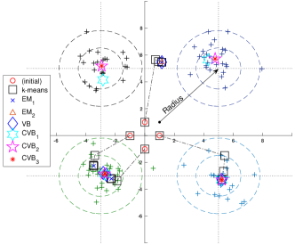
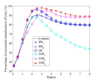
Figure 13: CVB and mean-field approximations for $K=4$ bivariate independent Normal clusters $\mathcal{N}(\boldsymbol{\mu},\mathbf{I}_{2})$, with mean vectors $\boldsymbol{\mu}$ located diagonally and equally at radius $R$ from the offset point $[1,1]^{T}$. The upper left panel shows the convergent results of approximated mean vectors for one Monte Carlo run in the case $R=4$, with true mean vectors located at intersections of four dotted lines. The dashed circles represent contours of true Normal distributions. The plus signs $+$ are $N=100$ random data, generated with equal probability from each Normal cluster. The four smallest circles are the same initial guesses of true mean vectors for all algorithms. The dash-dot line illustrates the k-means algorithm, from initial to convergent points. The other panels show the Purity, MSE and ELBO values at convergence with varying radius. The higher Purity, the higher percentage of correct classification of data. The higher ELBO at each radius, the lower KL divergence and, hence, the better approximation for that case of radius, as shown in (33-34) and illustrated in Fig. 7, 9. The number of Monte Carlo runs for each radius is $10^{4}$.

• Augmented CVB approximation:

As shown above, each value $j\in\{1,2,\ldots,N\}$ yields a different network structure for CVB approximation, as mentioned in section V. Let us consider here three simple ways to make use of these $N$ CVB’s structures.

The first and heuristic way, namely $\text{CVB}_{1}$ scheme, is to choose $\text{$\widehat{\boldsymbol{l}_{j}}$}(j)$ in (69), as the estimate for $j$-th label, because the CVB’s ternary structure is more focused on $\boldsymbol{l}_{j}$ at each $j\in\{1,2,\ldots,N\}$, as shown in Fig. 12. Since every $j$-th structure is equally important in this way, we can pick the empirical average $\widehat{\boldsymbol{\Upsilon}}\triangleq\sum_{j=1}^{N}\frac{1}{N}\widehat{\boldsymbol{\Upsilon}}(j)$ as estimate for cluster’s means.

The second way, namely $\text{CVB}_{2}$ scheme, is to pick $j$ such that $\text{KL}_{\widetilde{f}_{j}^{[\nu_{c}]}||f}$ at convergence is minimized, as mentioned in (40) . From (33-34), we then have $\widehat{j}\triangleq\operatornamewithlimits{arg\,min}_{j}\text{KL}_{\widetilde{f}_{j}^{[\nu_{c}]}||f}=\operatornamewithlimits{arg\,max}_{j}\text{ELBO}^{[\nu_{c}]}(j)=\operatornamewithlimits{arg\,max}_{j}\log\zeta_{2}^{[\nu_{c}]}(j)$, with $\zeta_{2}^{[\nu_{c}]}(j)$ given in (67). Then, $\widehat{\boldsymbol{l}_{i}}(\widehat{j})$ and $\widehat{\boldsymbol{\Upsilon}}(\widehat{j})$ in (69) will be used as estimates for categorical label $\boldsymbol{l}_{i}$ and cluster means, respectively, $\forall i\in\{1,2,\ldots,N\}$.

The third way, namely $\text{CVB}_{3}$ scheme, is to apply the augmented approach for CVB, given in (38). Then, from (41) and (69), the augmented CVB’s estimates for cluster’s means and labels in this case are $\widehat{\boldsymbol{\Upsilon}}^{*}\triangleq\sum_{j=1}^{N}q_{j}^{*}\widehat{\boldsymbol{\Upsilon}}(j)$ and $\widehat{\boldsymbol{l}_{i}}^{*}=\boldsymbol{\epsilon}_{\widehat{k_{i}}^{*}},$ respectively, with:

$$\widehat{k_{i}}^{*} \triangleq\operatornamewithlimits{arg\,max}_{k}\sum_{j=1}^{N}q_{j}^{*}\widetilde{q}_{k,i}^{[\nu_{c}]}(j),$$

$$q_{j}^{*} =\frac{\exp(-\text{KL}_{\widetilde{f}_{j}^{[\nu_{c}]}||f})}{\sum_{j=1}^{N}\exp(-\text{KL}_{\widetilde{f}_{j}^{[\nu_{c}]}||f})}=\frac{\zeta_{2}^{[\nu_{c}]}(j)}{\sum_{j=1}^{N}\zeta_{2}^{[\nu_{c}]}(j)},$$ (70)

in which $q_{j}^{*}$ is found via (38) and $\text{KL}_{\widetilde{f}_{j}^{[\nu_{c}]}||f}=-\text{ELBO}^{[\nu_{c}]}(j)+\log f(\boldsymbol{X}),$ as shown in (34) $\forall j\in\{1,2,\ldots,N\}$.

Although we can compute all moments of augmented CVB $\widetilde{f}_{0}^{[\nu_{c}]}=\sum_{j=1}^{N}q_{j}^{*}\widetilde{f}_{j}^{[\nu_{c}]}$via (41) and (70), it is difficult to evaluate $\text{KL}_{\widetilde{f}_{0}^{[\nu_{c}]}||f}$ and its ELBO value directly, as mentioned in subsection V-B. Hence, for comparison with $\text{CVB}_{2}$ scheme in simulations, let us instead compute heuristic values $\sum_{j=1}^{N}\frac{1}{N}\text{ELBO}^{[\nu_{c}]}(j)$ and $\sum_{j=1}^{N}q_{j}^{*}\text{ELBO}^{[\nu_{c}]}(j)$ at convergence for $\text{CVB}_{1}$ and $\text{CVB}_{3}$ schemes, respectively, with $\text{ELBO}^{[\nu_{c}]}(j)\triangleq\log\zeta_{2}^{[\nu_{c}]}(j)$ given in (67).

Remark 42.

Note that, the CVB $\widetilde{f}_{j}^{[\nu_{c}]}$ still belongs to a conditional structure class of node $j$ at convergence, even if the initialization $\{\widetilde{\boldsymbol{\mu}}_{k,m,j}^{[0]},\widetilde{\sigma}_{k,m,j}^{[0]}\}$ of CVB is exactly the same as that of VB. Indeed, in below simulations, even though initially we set $\widetilde{\boldsymbol{\mu}}_{k,m,j}^{[0]}=\widetilde{\boldsymbol{\mu}}_{k}^{[0]}$, $\widetilde{\sigma}_{k,m,j}^{[0]}=\widetilde{\sigma}_{k}^{[0]}$, $\forall m,j$ and, hence, $\widetilde{f}_{2|1}^{[0]}=\widetilde{f}^{[0]}(\boldsymbol{\Upsilon}|\boldsymbol{l}_{j},\boldsymbol{X})$ in (60) independent of $\boldsymbol{l}_{j}$, the conditional $\widetilde{f}^{[\nu]}(\boldsymbol{\Upsilon}|\boldsymbol{l}_{j},\boldsymbol{X})$ in (65-66) depends on $\boldsymbol{l}_{j}$ again in subsequent iterations, as already explained in subsection IV-B2 for this case of ternary partition.

VI-B5 Simulation’s results

Since k-means algorithm (50) works best for independent Normal clusters, let us illustrate the superior performance of CVB to mean-field approximations even in this case. For this purpose, a set of $K=4$ bivariate independent Normal clusters $\mathcal{N}(\boldsymbol{\mu}_{k},\mathbf{I}_{2})$ are generated randomly, with true means $\boldsymbol{\Upsilon}=\boldsymbol{\Upsilon}_{0}R+\left[\begin{array}[]{c}1\\ 1\end{array}\right]$ and $\boldsymbol{\Upsilon}_{0}\triangleq\left[\begin{array}[]{cccc}-1&1&1&-1\\ 1&1&-1&-1\end{array}\right]$. At each time $i$, a cluster is then chosen with equal probabilities $p_{k}=\frac{1}{K}$, $k\in\{1,2,\ldots,K\}$ in order to generate the data $\boldsymbol{x}_{i}\in\mathbb{R}^{2}$, $i\in\{1,2,\ldots,N\},$ with $N=100$, as shown in Fig. 13. The varying radius $R$ then controls the inter-distance between clusters. In order to quantify the algorithm’s performance, let us compute the Purity and mean squared error (MSE) for estimates $\widehat{\boldsymbol{l}}_{i}$, $\widehat{\boldsymbol{\Upsilon}}$ of categorical labels $\boldsymbol{l}_{i}$ and mean vectors $\boldsymbol{\Upsilon}$, respectively. The Purity, which is a common measure for percentage of successful label’s classification [53], is calculated as follows: $\text{Purity}=\sum_{k=1}^{K}\frac{1}{N}\max_{m}\sum_{i=1}^{N}\delta[\widehat{l}_{k,i}=l_{m,i}]$ in each Monte Carlo run. The higher $\text{Purity}\in[0,1]$, the better estimate for labels. The MSE in each Monte Carlo run is calculated as follows: $\text{MSE}=\frac{1}{K}\min_{\phi\in\Phi}||\phi(\widehat{\boldsymbol{\Upsilon}})-\boldsymbol{\Upsilon}||^{2}$, where $\Phi$ is all $K!$ possible permutations of $K$ estimated cluster means in $\widehat{\boldsymbol{\Upsilon}}\in\mathbb{R}^{2\times K}$.

For comparison at convergence, the initialization $\widetilde{\boldsymbol{\Upsilon}}^{[0]}=\boldsymbol{\Upsilon}_{0}$ and $\widetilde{\sigma}^{[0]}=1$ are the same for all algorithms. The k-means (50) and $\text{EM}_{1}$ algorithms (54) will converge at iteration $\nu_{c}$ if there is no update for categorical labels, i.e. $\widehat{\boldsymbol{L}}^{[\nu_{c}]}=\widehat{\boldsymbol{L}}^{[\nu_{c}-1]}\Leftrightarrow\text{ELBO}^{[\nu_{c}]}=\text{ELBO}^{[\nu_{c}-1]}$ in this case. The other algorithms are called converged at iteration $\nu_{c}$ if $0\leq\text{ELBO}^{[\nu_{c}]}-\text{ELBO}^{[\nu_{c}-1]}\leq 0.01$. The averaged values of $\nu_{c}$ over all cases in Fig. 13 are $[16.4,16.4,27.2,27.4,27.8]\pm[5.0,5.1,10.4,10.4,7.8]$ for k-means, $\text{EM}_{1}$, $\text{EM}_{2}$,VB and CVB algorithms. Only one approximated marginal is updated per iteration.

We can see that both performance and number of iterations of k-means and $\text{EM}_{1}$ algorithms are almost identical to each other, since they use the same approach with point estimates for categorical labels. Although the $\text{EM}_{1}$ (54) takes one extra data-driven step, in comparison with k-means, by using the total number of classified labels in each cluster as an indicator for credibility, the $\text{EM}_{1}$ is virtually the same as k-means in estimate’s accuracy. Likewise, since the point estimates of labels are data-driven and use hard decision approach, the k-means and $\text{EM}_{1}$ yield lower accuracy than other methods, which are model-driven and use soft decision approach.

The $\text{EM}_{2}$ (55) and VB (57) also have almost identical performance and number of iterations, even though $\text{EM}_{2}$ does not update the cluster mean’s credibility via total number of classified labels like VB does. Hence, like the case of $\text{EM}_{1}$ versus k-means, this extra step of data-driven update seems insignificant in terms of estimate’s accuracy. Nevertheless, since both $\text{EM}_{2}$ and VB use the model’s probability of each label as weighted credibility and make soft decision at each iteration, their performance is significantly better than k-means and $\text{EM}_{1}$ in the range of radius $R\in[2,4]$. Hence, the model-driven update step seems to exploit more information from the true model than the data-driven update step, when the clusters are close to each other.

For a large radius $R>4$, there is not much difference between soft and hard decisions for these standard Normal clusters, since the tail of Normal distribution is very small in these cases. Hence, given the same initialization at origin, the performances of all mean-field approximations like k-means, $\text{EM}_{1}$, $\text{EM}_{2}$ and VB are very close to each other when the inter-distance between clusters is high. Also, since the computation of soft decision in VB and $\text{EM}_{2}$ requires almost double number of iterations, compared with hard decision approaches like k-means and $\text{EM}_{1}$, the k-means is more advantageous in this case, owing to its low computational complexity.

The CVB algorithms are the slowest methods overall. Since the CVB in (70) requires nearly the same number of iterations as VB for each structure $j\in\{1,2,\ldots,N\}$, as illustrated in Fig. 12, the CVB’s complexity is at least $N$ times slower than VB method, where $N$ is the number of data. In practice, we may not have to update all $N$ CVB’s potential structures, since there might be some good candidates out of exponentially growing number of potential structures. In this paper, however, let us consider the case of $N$ structures in order to illustrate the superior performance of augmented CVB form in $\text{CVB}_{3}$ (70), in comparison with VB, heuristic $\text{CVB}_{1}$ and hit-or-miss $\text{CVB}_{2}$ approaches.

The heuristic $\text{CVB}_{1}$, which takes uniform average for mean vectors over all $N$ potential structures, returns a lower MSE than mean-field approximations in all cases. This result seems reasonable, since cluster means are common parameters of all potential CVB structures in Fig. 12. In contrast, $\text{CVB}_{1}$ returns label’s estimate $\widehat{\boldsymbol{l}}_{j}$ via $j$-th structure only, without considering label’s estimates from other CVB’s structures. Hence, the label’s Purity of $\text{CVB}_{1}$ is only on par with that of mean-field approximations for short radius $R\leq 2$ and deteriorates over longer radius $R>2$. As illustrated in Fig. 11, CVB might be the worst approximation if the CVB’s structure is too different from true posterior structure. In this case, a single $j$-th structure seems to be a bad CVB candidate for estimating label $\boldsymbol{l}_{j}$ at time $j\in\{1,2,\ldots,N\}.$

The hit-or-miss $\text{CVB}_{2}$, which picks the single best structure $\widehat{j}$ in terms of KL divergence, yields the worst performance in the range $R\in[1,2.5]$, while in other cases, it is the second-best method. The structure $\widehat{j}$, as illustrated in Fig. 12, concentrates on the $\widehat{j}$-th label. Hence, the classification’s accuracy of $\text{CVB}_{2}$ depends on whether the hard decision on $\widehat{j}$-th label serves as a good reference for other labels, as illustrated in Fig. 11. For this reason, $\text{CVB}_{2}$ may be able to achieve globally optimal approximation, but it may also be worse than mean-field approximations. When $R<3$, which is less than three standard deviation of a standard Normal cluster, the clusters data are likely overlapped with each other. Within this range, the hard decision of $\text{CVB}_{2}$ on $\widehat{j}$ destroys the correlated information between clusters and, hence, becomes worse than other methods. For $R\geq 3$, the $\text{CVB}_{2}$ becomes better, which indicates that the classification’s accuracy now relies more on the most significantly correlated structure between labels.

Generalizing both schemes $\text{CVB}_{1}$ and $\text{CVB}_{2}$, $\text{CVB}_{3}$ (70) can return the optimal weights for the mixture of $N$ potential structures and achieve the minimum upper bound of KL divergence (37), as illustrated in Fig. 4. Hence, the $\text{CVB}_{3}$ yields the best performance in Fig. 13. When $R<3$, the $\text{CVB}_{3}$ is on par with VB approximation, since the probabilities computed via Normal model are high enough for making soft decisions in VB. When $R>3$, however, VB has to rely on hard decisions like k-means, since the standard Normal probabilities are too low. The $\text{CVB}_{3}$, in contrast, automatically move the mixture’s weights closer to hard decision on the best structures like $\text{CVB}_{2}$.

Note that, although the computed ELBO values for $\text{CVB}_{2}$ in Fig. 13 are correct, the computed ELBO values for $\text{CVB}_{1}$ and $\text{CVB}_{3}$ are merely heuristic and not correct values, since their ELBO values are hard to compute in this case. Nonetheless, from their performance in Purity and MSE, we may speculate that the true ELBO values of $\text{CVB}_{1}$ and $\text{CVB}_{3}$ are lower and higher than those of $\text{CVB}_{2}$, respectively. Equivalently, in terms of KL divergence, the $\text{CVB}_{3}$ seems to be the best posterior approximation for this independent Normal cluster model, followed by $\text{CVB}_{2}$, $\text{CVB}_{1}$ and mean-field approximations, which yield almost identical ELBO values.

Intuitively, as shown in the case of $R=4$ in the upper left panel of Fig. 13, the mean-field approximations like VB, EM and k-means seems not to recognize the correlations between data of the same clusters, but focus more on the inter-distance between clusters as a whole. The CVB approximations, in contrast, exploit the correlations between each label $\boldsymbol{l}_{j}$ to all other labels, as shown in Fig. 12. Although the heuristic $\text{CVB}_{1}$ becomes worse when $R$ increases, the $\text{CVB}_{2}$ and $\text{CVB}_{3}$ are still able to pick the best correlated structures to represent the data. When inter-distance of cluster is much higher than cluster’s variance, these two CVB methods stabilize and accurately classify $90\%$ of total data in average. The successful rate is only about $80\%$ for all other state-of-the-art mean-field approximations.

VII Conclusion

In this paper, the independent constraint of mean-field approximations like VB, EM and k-means algorithms has been shown to be a special case of a broader conditional constraint class, namely copula. By Sklar’s theorem, which guarantees the existence of copula for any joint distribution, a copula Variational Bayes (CVB) algorithm is then designed in order to minimize the Kullback-Leibler (KL) divergence from the true joint distribution to an approximated copula class. The iterative CVB can converge to the true probability distribution when their copula structures are close to each other. From perspective of generalized Bregman divergence in information geometry, the CVB algorithm and its special cases in mean-field approximations have been shown to iteratively project the true probability distribution to a conditional constraint class until convergence at a local minimum KL divergence.

For a global approximation of a generic probabilistic network, the CVB is then further extended to the so-called augmented CVB form. This global CVB network can be seen as an optimally weighted hierarchical mixture of many local CVB approximations with simpler network structures. By this way, the locally optimal approximation in mean-field methods can be extended to be globally optimal in copula class for the first time. This global property was then illustrated via simulations of correlated bivariate Gaussian distribution and standard Normal clustering, in which the CVB’s performance was shown to be far superior to VB, EM and k-means algorithms in terms of percentage of accurate classifications, mean squared error (MSE) and KL divergence. Despite being canonical, these popular Gaussian models illustrated the potential applications of CVB to machine learning and Bayesian network. The application of copula’s design in statistics and a faster computational flow for augmented CVB network may be regarded as two out of many promising approaches for improving CVB approximation in future works.

Appendix A Bayesian minimum-risk estimation

Let us briefly review the importance of posterior distributions in practice, via minimum-risk property of Bayesian estimation method. Without loss of generalization, let us assume that the unknown parameter $\theta$ in our model is continuous. In practice, the aim is often to return estimated value $\hat{\theta}\triangleq\hat{\theta}(\boldsymbol{x})$, as a function of noisy data $\boldsymbol{x}$, with least mean squared error $\text{MSE}(\hat{\theta},\theta)\triangleq\mathbb{E}_{f(\boldsymbol{x},\theta)}||\hat{\theta}(\boldsymbol{x})-\theta||^{2}$, where $||\cdot||$ is $\mathcal{L}_{2}$-normed operator. Then, by basic chain rule of probability $f(\boldsymbol{x},\theta)=f(\theta|\boldsymbol{x})f(\boldsymbol{x})$, we have [45, 1]:

$$\hat{\theta} \triangleq\operatornamewithlimits{arg\,min}_{\tilde{\theta}}\text{MSE}(\tilde{\theta},\theta)$$

$$=\operatornamewithlimits{arg\,min}_{\tilde{\theta}}\mathbb{E}_{f(\theta|\boldsymbol{x})}||\tilde{\theta}(\boldsymbol{x})-\theta||^{2}$$ (71)

$$=\mathbb{E}_{f(\theta|\boldsymbol{x})}(\theta),$$

which shows that the posterior mean $\hat{\theta}=\mathbb{E}_{f(\theta|\boldsymbol{x})}(\theta)$ is the least MSE estimate. Note that, the result (71) is also a special case of Bregman variance theorem (7) when applied to Euclidean distance (8). In general, we may replace the $\mathcal{L}_{2}$-norm in (71) by other normed functions. For example, it is well-known that the best estimators for the least total variation norm $\mathcal{L}_{1}$ and the zero-one loss $\mathcal{L}_{\infty}$ are the median and mode of the posterior $f(\theta|\boldsymbol{x})$, respectively [45, 1].

Viet Hung Tran received the B.Eng. degree from Hochiminh city University of Technology, Vietnam, in 2008, the master‘s degree from ENS Cachan, Paris, France, in 2009, and the Ph.D. degree from the Trinity College Dublin, Ireland, in 2014. From 2014 to 2016, he held a post-doctoral position with Telecom ParisTech. He is currently a Research Fellow at University of Surrey, London suburb, U.K. His research interest is optimal algorithms for Bayesian learning network and information theory. He was awarded the best mathematical paper prize at IEEE Irish Signals and Systems Conference, 2011.

References

- [1] V. H. Tran, “Variational Bayes inference in digital receivers,” Ph.D. dissertation, Trinity College Dublin, 2014.
- [2] V. Smidl and A. Quinn, The Variational Bayes Method in Signal Processing. Springer, 2006.
- [3] M. Beal, “Variational algorithms for approximate Bayesian inference,” Ph.D. dissertation, University College London, Jun. 2003.
- [4] S. Watanabe and J.-T. Chien, Bayesian Speech and Language Processing. Cambridge University Press, 2015.
- [5] T. Bayes, “An essay towards solving a problem in the doctrine of chances,” Philosophical Transactions of the Royal Society of London, vol. 53, pp. 370–418, 1763.
- [6] S. M. Stigler, The History of Statistics: The Measurement of Uncertainty Before 1900. Harvard University Press, 1986.
- [7] M. Karny and K. Warwick, Eds., Computer Intensive Methods in Control and Signal Processing - The Curse of Dimensionality. Birkhauser, Boston, MA, 1997.
- [8] A. Graves, “Practical variational inference for neural networks,” Advances in Neural Information Processing Systems (NIPS), 2011.
- [9] L. He, H. Chen, and L. Carin, “Tree-structured compressive sensing with Variational Bayesian analysis,” IEEE Signal Processing Letters, vol. 17, no. 3, pp. 233–236, Mar. 2010.
- [10] S. Subedi and P. D. McNicholas, “Variational Bayes approximations for clustering via mixtures of normal inverse Gaussian distributions,” Advances in Data Analysis and Classification, vol. 8, no. 2, pp. 167–193, Jun. 2014.
- [11] M. J. Wainwright and M. I. Jordan, “Graphical models, exponential families, and variational inference,” Foundations and Trends in Machine Learning, vol. 1, no. 1-2, pp. 1–305, Nov. 2008.
- [12] J. S. Yedidia, W. T. Freeman, and Y. Weiss, “Constructing free-energy approximations and generalized belief propagation algorithms,” IEEE Transactions on Information Theory, vol. 51, no. 7, pp. 2282–2312, Jul. 2005.
- [13] A. Sklar, “Fonctions de répartition à N dimensions et leurs marges,” Publications de l’Institut Statistique de l’Université de Paris, vol. 8, pp. 229–231, 1959.
- [14] F. Durante and C. Sempi, Principles of Copula Theory. Chapman and Hall/CRC, 2015.
- [15] A. Kolesarova, R. Mesiar, J. Mordelova, and C. Sempi, “Discrete copulas,” IEEE Transactions on Fuzzy Systems, vol. 14, no. 5, pp. 698–705, Oct. 2006.
- [16] A. Sklar, “Random variables, distribution functions, and copulas - a personal look backward and forward,” in Distributions with fixed marginals and related topics, ser. Lecture Notes-Monograph, L. Ruschendorf, B. Schweizer, and M. D. Taylor, Eds., vol. 28. Institute of Mathematical Statistics, Hayward, CA, 1996, pp. 1–14.
- [17] X. Zeng and T. Durrani, “Estimation of mutual information using copula density function,” IEEE Electronics Letters, vol. 47, no. 8, pp. 493–494, Apr. 2011.
- [18] S. Grønneberg and N. L. Hjort, “The copula information criteria,” Scandinavian Journal of Statistics, vol. 41, no. 2, pp. 436–459, 2014.
- [19] L. A. Jordanger and D. Tjøstheim, “Model selection of copulas - AIC versus a cross validation copula information criterion,” Statistics and Probability Letters, vol. 92, pp. 249–255, Jun. 2014.
- [20] S. ichi Amari, Information Geometry and Its Applications. Springer Japan, Feb. 2016.
- [21] P. Stoica and Y. Selen, “Cyclic minimizers, majorization techniques, and the Expectation-Maximization algorithm - a refresher,” IEEE Signal Processing Magazine, vol. 21, no. 1, pp. 112–114, Jan. 2004.
- [22] Y. Sun, P. Babu, and D. P. Palomar, “Majorization-Minimization algorithms in signal processing, communications, and machine learning,” IEEE Transactions on Signal Processing, vol. 65, no. 3, pp. 794–816, Feb. 2017.
- [23] J. Besag, “On the statistical analysis of dirty pictures,” Journal of the Royal Statistical Society, vol. B-48, pp. 259–302, 1986.
- [24] A. Dogandzic and B. Zhang, “Distributed estimation and detection for sensor networks using hidden Markov random field models,” IEEE Transactions on Signal Processing, vol. 54, no. 8, pp. 3200–3215, 2006.
- [25] S. P. Lloyd, “Least squares quantization in PCM,” IEEE Transactions on Information Theory, vol. 28, no. 2, pp. 129–137, Mar. 1982.
- [26] C. Boutsidis, A. Zouzias, M. W. Mahoney, and P. Drineas, “Randomized dimensionality reduction for k-means clustering,” IEEE Transactions on Information Theory, vol. 61, no. 2, pp. 1045–1062, Feb. 2015.
- [27] V. H. Tran, “Cost-constrained Viterbi algorithm for resource allocation in solar base stations,” IEEE Transactions on Wireless Communications, vol. 16, no. 7, pp. 4166–4180, Apr. 2017.
- [28] T. Jebara and A. Pentland, “On reversing Jensen’s inequality,” Advances in Neural Information Processing Systems 13 (NIPS), pp. 231–237, 2001.
- [29] P. Carbonetto and N. de Freitas, “Conditional mean field,” Proceedings of the 19th International Conference on Neural Information Processing Systems (NIPS), pp. 201–208, Dec. 2006.
- [30] E. P. Xing, M. I. Jordan, and S. Russell, “A generalized mean field algorithm for variational inference in exponential families,” Proceedings of the Nineteenth conference on Uncertainty in Artificial Intelligence (UAI), pp. 583–591, Aug. 2003.
- [31] D. Geiger, C. Meek, and C. Meek, “Structured variational inference procedures and their realizations,” Proceedings of Tenth International Workshop on Artificial Intelligence and Statistics, 2005.
- [32] D. Tran, D. M. Blei, and E. M. Airoldi, “Copula variational inference,” 28th International Conference on Neural Information Processing Systems (NIPS), vol. 2, pp. 3564–3572, Dec. 2015.
- [33] B. A. Frigyik, S. Srivastava, and M. R. Gupta, “Functional Bregman divergence and Bayesian estimation of distributions,” IEEE Transactions on Information Theory, vol. 54, no. 11, pp. 5130–5139, Nov. 2008.
- [34] J.-D. Boissonnat, F. Nielsen, and R. Nock, “Bregman voronoi diagrams,” Discrete & Computational Geometry (Springer), vol. 44, no. 2, pp. 281–307, Sep. 2010.
- [35] A. Banerjee, S. Merugu, I. S. Dhillon, and J. Ghosh, “Clustering with Bregman divergences,” Journal of Machine Learning Research, vol. 6, pp. 1705–1749, Oct. 2005.
- [36] S. ichi Amari, “Divergence, optimization and geometry,” International Conference on Neural Information Processing, pp. 185–193, 2009.
- [37] M. Adamcík, “The information geometry of Bregman divergences and some applications in multi-expert reasoning,” Entropy, vol. 16, no. 12, pp. 6338–6381, Dec. 2014.
- [38] M. A. Proschan and P. A. Shaw, Essentials of Probability Theory for Statisticians. Chapman and Hall/CRC, Apr. 2016.
- [39] F. Nielsen and R. Nock, “Sided and symmetrized Bregman centroids,” IEEE Transactions on Information Theory, vol. 55, no. 6, pp. 2882–2904, Jun. 2009.
- [40] B. A. Frigyik, S. Srivastava, and M. R. Gupta, “An introduction to functional derivatives,” Department of Electronic Engineering, University of Washington, Seattle, WA, Tech. Rep. 0001, 2008.
- [41] U. Cherubini, E. Luciano, and W. Vecchiato, Copula Methods in Finance. John Wiley & Sons, Oct. 2004.
- [42] J.-F. Mai and M. Scherer, Financial Engineering with Copulas Explained. Palgrave Macmilan, 2014.
- [43] A. Shemyakin and A. Kniazev, Introduction to Bayesian Estimation and Copula Models of Dependence. Wiley-Blackwell, May 2017.
- [44] S. Han, X. Liao, D. Dunson, and L. Carin, “Variational Gaussian copula inference (and supplementary materials),” Proceedings of the 19th International Conference on Artificial Intelligence and Statistics, vol. 51, pp. 829–838, May 2016.
- [45] J. M. Bernardo and A. F. M. Smith, Bayesian Theory. John Wiley & Sons Canada, 2006.
- [46] D. M. Blei, A. Kucukelbir, and J. D. McAuliffe, “Variational inference - a review for statisticians,” Journal of the American Statistical Association, vol. 112, no. 518, pp. 859–877, Feb. 2017.
- [47] J. Winn and C. M. Bishop, “Variational message passing,” Journal of Machine Learning Research, vol. 6, pp. 661–694, Apr. 2005.
- [48] D. G. Tzikas, A. C. Likas, and N. P. Galatsanos, “The variational approximation for Bayesian inference,” IEEE Signal Processing Magazine, vol. 25, no. 6, pp. 131–146, Nov. 2008.
- [49] M. Sugiyama, Introduction to Statistical Machine Learning. Elsevier, 2015.
- [50] D. J. MacKay, Information Theory, Inference, and Learning Algorithms. Cambridge University Press, 2003.
- [51] R. Ranganath, D. Tran, and D. M. Blei, “Hierarchical variational models,” 33rd International Conference on International Conference on Machine Learning (ICML), vol. 48, pp. 2568–2577, Jun. 2016.
- [52] D. Tran, R. Ranganath, and D. Blei, “Hierarchical implicit models and likelihood-free variational inference,” Advances in Neural Information Processing Systems (NIPS), pp. 5529–5539, Dec. 2017.
- [53] P.-N. Tan, M. Steinbach, and V. Kumar, Introduction to Data Mining. Addison-Wesley, Boston, 2006.