Error Analysis and Improving the Accuracy of Winograd Convolution for Deep Neural Networks

Abstract.

Popular deep neural networks (DNNs) spend the majority of their execution time computing convolutions. The Winograd family of algorithms can greatly reduce the number of arithmetic operations required and is present in many DNN software frameworks. However, the performance gain is at the expense of a reduction in floating point (FP) numerical accuracy. In this paper, we analyse the worst case FP error and prove the estimation of norm and conditioning of the algorithm. We show that the bound grows exponentially with the size of the convolution, but the error bound of the modified algorithm is smaller than the original one. We propose several methods for reducing FP error. We propose a canonical evaluation ordering based on Huffman coding that reduces summation error. We study the selection of sampling “points” experimentally and find empirically good points for the most important sizes. We identify the main factors associated with good points. In addition, we explore other methods to reduce FP error, including mixed-precision convolution, and pairwise summation across DNN channels. Using our methods we can significantly reduce FP error for a given block size, which allows larger block sizes and reduced computation.

1. Motivation

Deep Neural Networks (DNNs) have become powerful tools for image, video, speech and language processing. However, DNNs are very computationally demanding, both during and after training. A large part of this computations consists of convolution operations, which are used across a variety of DNNs, and in particular convolutional neural networks (CNNs). As DNNs become ubiquitous, reducing the cost of DNN convolution is increasingly important.

Simple direct convolution require $O(n^{2})$ operations to convolve a size $n$ input with size $n$ convolution kernel. In contrast, fast convolution algorithms require asymptotically fewer operations. For example, converting the kernel and input to the Fourier domain with the fast Fourier transform (FFT) requires just $O(nlog_{2}(n))$ operations. In the Fourier domain, convolution can be computed in $O(n)$ operations by pairwise multiplication (Hadamard product) of the input vectors.

Although FFT convolution is a popular approach, within the area of deep neural networks (DNNs) a less well known algorithm is widely used. The Winograd family of fast convolution algorithms attempts to minimize the number of operations needed for fixed-size small convolutions. Around 1980, Winograd proved that a convolution of the input of length $n$ with a kernel of length $n_{h}$ can be computed using a theoretical minimum of just $n+n_{h}-1$ general multiplications (Hadamard product operations) [31].

Winograd convolutions use a predetermined triple of linear transforms. The first two transform the input and the kernel to space where, like in the Fourier domain, pointwise multiplication (Hadamard product) can be used to perform convolution. The third transform moves the result back to the space of the inputs. In Winograd convolution, each of the transforms requires $O(n^{2})$ operations, as compared to $O(nlog_{2}(n))$ for FFT. Thus, Winograd convolution is efficient only for very small convolutions, or where the cost of the transform can be amortized over many uses of the transformed data. In DNN convolution, the kernels are small, typically $3\times 3$ or $5\times 5$, and large inputs can be broken into a sequence of smaller segments. Further, each input is convolved with many kernels, and each kernel with many input segments, so the cost of transform operations is amortized over multiple uses. Further, DNNs often operate on a mini-batch of many inputs (typically 32–512) at a time, which further increases the re-use of each transformed kernel.

Although the transforms are expensive, Winograd convolution can guarantee the theoretical minimum number of general multiplications. The Winograd transform of a real-valued input is real-valued, so that real (not complex) multiplication is used for pairwise multiplication (Hadamard product). Real-valued multiplication requires just one machine multiply, whereas complex multiplication requires four multiplies and two adds, or three multiplies and five adds [17]. Compared with the FFT approach, Winograd convolution allows for faster Hadamard product computations, at the cost of more expensive transforms.

Winograd convolution has a further weakness. The linear transforms are pathologically bad cases for FP accuracy, as we describe in Section 4. To obtain a good level of numerical accuracy it is normally necessary to break convolutions with a large input into a sequence of smaller ones. However, recall that Winograd convolution requires $n+h_{h}-1$ general multiplications to convolve an input of size $n$ with a kernel of size $n_{h}$. Thus, when a large input is split into segments, there is an overhead of $n_{h}-1$ additional general multiplications for each segment.

In this paper, we address the question of numerical accuracy of Winograd convolution for deep neural networks. Better numerical accuracy allows inputs to be split into a smaller number of larger segments, which in turn reduces the number of general multiplications. We take both analytical and experimental approaches to the problem. We isolate the components of error which can be identified with mathematical analysis, and establish empirical bounds for the components which cannot. We make the following specific contributions.

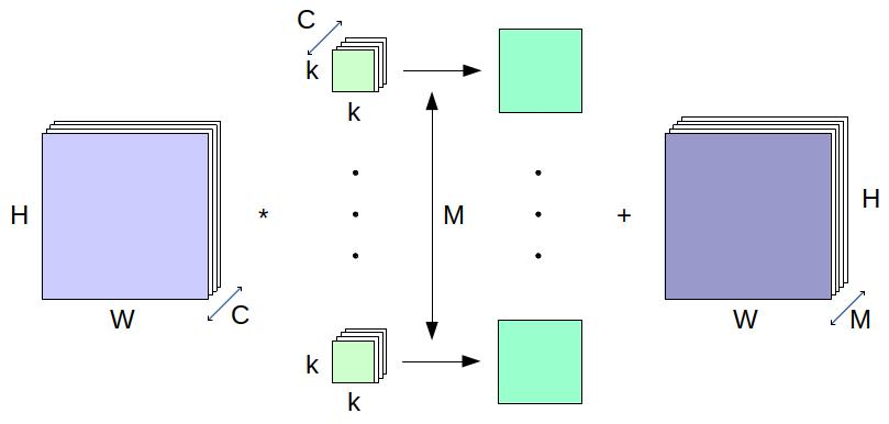
Figure 1. Diagram of the structure of DNN convolution. 2D convolutions are computed between kernels of size $k\times k$ and inputs of size $H\times W$. Bundles of $C$ such convolution are summed pointwise to produce 1 output. $M$ outputs are produced this way, and concatenated along the $M$ index to produce the input for the next operation.

• We formalize and prove worst-case FP error bounds and identify error terms for the Toom-Cook algorithm, and show that error grows at least exponentially.

• We present a formal analysis of the error bounds for the “modified” Toom-Cook algorithm, and prove that it has a lower, but nonetheless exponentially-growing error.

• We estimate the algorithm norm and conditioning.

• We demonstrate that order of evaluation of FP expressions in the linear transform impacts accuracy. We propose a canonical Huffman tree evaluation order that reduces average error at no additional cost in computation.

• We experimentally evaluate strategies for selecting algorithm coefficients for typical DNN convolutions. We show relationships between coefficients which improve accuracy.

• We investigate algorithms that use a higher (double) precision transform. These methods reduce the error typically by around one third in our experiments.

2. Fast Convolution and Deep Neural Networks

In DNN convolution, each input segment (or kernel) is typically convolved with many kernels (or input segments). When the 2D convolutions are implemented with a fast convolution algorithm, the transforms are thus amortized over many reuses of the transformed segments. Therefore, we are primarily interested in convolution algorithms that minimize the general multiplications which implement the pairwise multiplication (Hadamard product) step.

Winograd [31] proved that the minimum number of general multiplications (that is the multiplications used in the Hadamard product) is $n+n_{h}-1$. Winograd demonstrated that the existing Toom-Cook method [26, 6] is capable of generating optimal convolution algorithms that achieve this minimum. Winograd also developed his own method for generating fast algorithms.

In 2016 Lavin and Gray [18] demonstrated that Winograd convolution can be around twice as fast as direct convolution in DNNs [18]. A key contribution of their paper is an algorithm to break multi-channel multi-kernel DNN convolution into smaller segments that can be computed with matrix multiplication. Lavin and Gray actually used the Toom-Cook rather than Winograd’s method to generate their convolution algorithms. However, they described their approach as “Winograd convolution” and within the DNN research literature that term has come to include both Toom-Cook and Winograd methods.

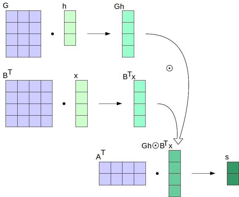
Figure 2. Toom-Cook Convolution. The forward linear transform of kernel $h$ is computed by multiplication with matrix $G$. Similarly, the forward linear transform of input $x$ is computed by multiplication with a matrix $B^{T}$. Corresponding elements of the two resulting vectors are then multiplied pairwise (compute Hadamard product) to perform the convolution. The resulting vector is the image under the linear transform of the actual convolution output. To translate the result back to the domain of the inputs, $h$ and $x$, the backward transform is applied by multiplication with a matrix $A^{T}$ to produce the final output $s$.

2.1. Decomposing Convolution and Minimizing General Multiplications

A convolution of any output size $n_{o}>1$ can be decomposed into the sum of smaller convolutions. For example, a convolution with $n_{o}=8$ can be computed as eight convolutions with $n_{o}=1$ (i.e. direct convolution), four convolutions with $n_{o}=2$, two convolutions with $n_{o}=4$, or one convolution with $n_{o}=8$. With a kernel of size $n_{h}=3$, the total number of general multiplications for each of these decompositions will be $8\times 3=24$, $4\times 4=16$, $2\times 6=12$ or $1\times 10=10$ respectively.

The larger the size of each sub-convolution, the fewer general multiplications are needed to compute the total output. Unfortunately, bigger output sizes lead to larger FP errors. In fact, as we show in Section 4, the error grows at least exponentially with $n_{o}+n_{h}-1$.

Table 1 summarizes the number of general multiplications per output point for different output block sizes using a selection of typical kernel sizes from real-world DNNs. Clearly, we would like to benefit from the efficiency of large output block sizes. For example, a $5\times 5$ Toom-Cook convolution with an output block size of $12\times 12$ (bottom right) uses around $14\times$ fewer general multiplications per output point than direct convolution (top right). However, the error for $n_{h}=5\times 5$ is so large, that in practice sizes $n_{o}>3\times 3$ are not used in any current DNN software framework.

Table 1. Number of multiplications per single output point for direct and Toom-Cook convolutions for different kernel and output size

No of	Output	Mult/	Output size	Mult/	Output	Mult/	Output	Mult/
points	$K=3$	output	$K=3\times 3$	output	for $K=5$	output	$K=5\times 5$	output
0	1	3	1$\times$1	9	1	5	1$\times$1	25
4	2	2	2$\times$2	4	-	-	-	-
5	3	1.67	3$\times$3	2.78	-	-	-	-
6	4	1.5	4$\times$4	2.25	2	3	2$\times$2	9
7	5	1.4	5$\times$5	1.96	3	2.33	3$\times$3	5.44
8	6	1.34	6$\times$6	1.78	4	2	4$\times$4	4
9	7	1.29	7$\times$7	1.65	5	1.8	5$\times$5	3.24
10	8	1.25	8$\times$8	1.56	6	1.67	6$\times$6	2.78
11	9	1.22	9$\times$9	1.49	7	1.57	7$\times$7	2.47
12	10	1.2	10$\times$10	1.44	8	1.5	8$\times$8	2.25
13	11	1.18	11$\times$11	1.4	9	1.44	9$\times$9	2.09
14	12	1.17	12$\times$12	1.36	10	1.4	10$\times$10	1.96
15	13	1.15	13$\times$13	1.33	11	1.36	11$\times$11	1.86
16	14	1.14	14$\times$14	1.31	12	1.33	12$\times$12	1.78

3. Toom-Cook algorithm

In this section we describe the Toom-Cook convolution algorithm. It is based on the Chinese Remainder Theorem (CRT) for polynomials and the Matrix Exchange Theorem. Toom [26] and Cook [6] provide details on the theoretical background. Parhi [20], Tolimieri [25] and Blahut [4] provide useful descriptions of using the Toom-Cook algorithm to perform a discrete convolution. The one-dimensional discrete convolution of two vectors $h\begin{bmatrix}h_{1}&\cdots&h_{n_{h}}\end{bmatrix}$ and $x=\begin{bmatrix}x_{1}&\cdots&x_{n}\end{bmatrix}$ is the vector $s=h\ast x$ where $s_{i}=\sum_{j=1}^{i}h_{i}x_{i-j}$.

The main idea of Toom-Cook convolution is to transform the kernel and input into the modulo polynomial domain where convolution becomes an element-wise multiplication (Hadamard product) and then transform the result back. We construct three matrices, one for the kernel transform, one for the input transform, and one to transform the result back. We denote these matrices as $G$, $A$ and $B$ respectively.

Theorem 1 (Chinese Remainder Theorem for polynomials).

Let $\mathbb{F}[a]$ be the ring of all polynomials over a field $\mathbb{F}$. Consider the polynomial $M(a)\in\mathbb{F}[a]$ such as $M(a)=m_{1}(a)...m_{\ell}(a)$ where $m_{i}(a)$ irreducible $\forall i=1,2,..,\ell$ and $GCD(m_{i}(a),m_{j}(a))=1$ $\forall i=1,2,..,\ell,\ i\neq j$. Let $s_{i}(a)\in\mathbb{F}[a]$ be any polynomials for $i=1,2,..,\ell$. Then there exists $s(a)\in\mathbb{F}[a]$ a unique solution of the system of congruences:

$$s(a)=s_{i}(a)\;mod\;m_{i}(a)\qquad\forall\ i=1,2,..,\ell$$

and

$$s(a)=\sum_{i=1}^{\ell}s_{i}(a)N_{i}(a)M_{i}(a)\;mod\;M(a)$$

where:

$$N_{i}(a)M_{i}(a)+n_{i}(a)m_{i}(a)=1,\qquad N_{i}(a),\;M_{i}(a)=\frac{M(a)}{m_{i}(a)},\ \mbox{and}\qquad m_{i}(a)\in\mathbb{F}[a].$$

Let us assume in what follows that $\mathbb{F}$ is equal to $\mathbb{R}$, a field of real numbers, and represent the one-dimensional kernel vector $h=\begin{bmatrix}h_{1}&h_{2}&\cdots&h_{n_{h}}\end{bmatrix}$ and one-dimensional input vector $x=\begin{bmatrix}x_{1}&x_{2}&\cdots&x_{n}\end{bmatrix}$ as polynomials $h(a)$ and $x(a)$, with coefficients equal to their respective components, such that the leading coefficients of $h(a)$ and $x(a)$ are taken to be $h_{n_{h}}$ and $x_{n}$, respectively. Then computing the one-dimensional discrete convolution is equivalent to computing the coefficients of the polynomial product $s(a)=h(a)x(a)$.

In the Toom-Cook algorithms, it is assumed that all $m^{(i)}(a)$ are monomials; so the computation reduces to the following steps:

1. Choosing points $p_{i}$ to construct polynomials $m_{i}(a)=a-p_{i}$;

2. Evaluating polynomials $h(a)$, $x(a)$ at each point $p_{i}$ to change the domain, which is equivalent to computing $h_{i}(a)=h(a)\;mod\;m_{i}(a)$ and $x_{i}(a)=x(a)\;mod\;m_{i}(a)$;

3. Performing the multiplication $s_{i}(a)=h_{i}(a)x_{i}(a)$; and

4. Applying the Chinese Reminder Theorem to compute the coefficients of the polynomial $s_{i}$.

We can represent this algorithm as:

$$V^{-1}(V_{x}x\odot V_{h}h)$$

where matrices $V_{x}$ and $V_{h}$ (called Vandermonde matrices) represent transformation into the modulo polynomial domain, which is equivalent to evaluation of the polynomial in different points $p_{i}$. The matrix $V^{-1}$ is the inverse Vandermonde matrix for the transformation of the result back from the modulo polynomial domain. The nonsingularity of these matrices is guaranteed by choosing the different $a_{i}$ so that the assumptions of the CRT are fulfilled.

3.1. Matrix Interchange

It is possible to interchange matrices in the convolution formula using the Matrix Exchange theorem.

Theorem 2.

Let $M$ be a diagonal matrix. If matrix $M$ can be factorised as $M=CDE$ then it also can be factorised as $M=(\overline{E})^{T}D(\underline{C})^{T}$, where matrix $\overline{E}$ is a matrix obtained from $E$ by reversing the order of its columns and $\underline{C}$ is a matrix obtained from $C$ by reversing its rows.

Although the literature on DNNs typically calls this operation convolution, from a mathematical point of view the operation we want to compute is, in fact, the correlation. This is why, when applying the Matrix Exchange Theorem, we do not reverse the order of columns in matrix $E$. Thus

$$V^{-1}(V_{x}x\odot V_{h}h)=V^{-1}Diag(V_{h}h)V_{x}x={V_{x}}^{T}(V_{h}h\odot V^{-T}x)$$

Putting $A=V_{x}$, $G=V_{h}$ and $B=V^{-1}$ we obtain the following formula for one-dimensional convolution

$$(h\ast x)_{1D}=A^{T}(Gh\odot B^{T}x)$$

In a similar way, using the Kronecker product, we obtain a formula for two-dimensional convolution

$$(H\ast X)_{2D}=A^{T}(GHG^{T}\odot B^{T}XB)A$$

where matrices $H$ and $X$ are the two-dimensional kernel and input, respectively.

3.2. Linear Transform Matrix Construction

The method of constructing matrices $A^{T}$, $G$ and $B^{T}$ is presented in Algorithm 1. To compute a 1D convolution of size $n_{o}$ with the kernel of size $n_{h}$, we need a input of size $n=n_{h}+n_{o}-1$. As inputs to the algorithm we provide $n$ different real points $p_{1},..,p_{n}$ and use them to construct $n$ linear polynomials $m_{i}(a)=x-p_{i}$, for $i=1,..,n$. We compute polynomial $M(a)=(a-p_{1})..(a-p_{n})$ and polynomials $M_{i}(a)=M(a)/m_{i}(a)=\sum_{j}{M_{j,i}a^{j-1}}$ for $i=1,2,\ldots,n$ and $j=0,1,\ldots,n$ used in CRT.

The matrix $A^{T}$ is a transposed rectangular Vandermonde matrix of size $n_{o}\times n$. We compute its elements as the $0$th to $n_{o}-1$th powers of the $n$ selected points. Next, we construct the matrix $G$ of size $n\times n_{h}$ in a very similar way. Note that we scale one of the Vandermonde matrices by coefficients $N_{i}$ to obtain matrices $G$ and $B^{T}$. We find the coefficients $N_{i}$ using the Euclidean algorithm [2].

Input: $n_{o}$ - size of output, $n_{h}$ - size of kernel, ;

$\{p_{1},\cdots,p_{n}\}$ set of $n$ different points

Output: Three matrices $A^{T}$, $G$ $B^{T}$ for Toom-Cook convolution

1 $n=n_{o}+n_{h}-1$;

2 for $i=1$ to $n$ do

3      for $j=1$ to $n$ do

4           $M_{i,j}$ = coefficient of the polynomial $\prod_{k\neq i}({a-p_{k}})$ stands for $a^{j-1}$

5          

6           for $i=1$ to $n$ do

7                $N_{i}=\frac{1}{\prod_{j\neq i}(p_{i}-p_{j})}$

8                for $i=1$ to $n_{o}$ do

9                     for $j=1$ to $n$ do

10                          $A^{T}_{i,j}={p_{j}}^{i-1}$

11                         

12                          for $i=1$ to $n$ do

13                               for $j=1$ to $n_{h}$ do

14                                    $G_{i,j}={p_{i}}^{j-1}*N_{i}$

15                                   

16                                    for $i=1$ to $n$) do

17                                         for $j=1$ to $n$ do

18                                              $B^{T}_{i,j}=M_{j,i}$

19                                             

ALGORITHM 1 Toom-Cook algorithm

The general form of matrices obtained by the Toom-Cook algorithm is as follows:

$${G=\begin{bmatrix}1&p_{1}*N_{1}&\cdots&{p_{1}}^{n_{h}-1}*N_{1}\\ 1&p_{2}*N_{2}&\cdots&{p_{2}}^{n_{h}-1}*N_{2}\\ \vdots&\vdots&\ddots&\vdots\\ 1&p_{n}*N_{n}&\cdots&{p_{n}}^{n_{h}-1}*N_{n}\end{bmatrix};\ \ A^{T}=\begin{bmatrix}1&1&\cdots&1\\ p_{1}&p_{2}&\cdots&p_{n}\\ \vdots&\vdots&\ddots&\vdots\\ p_{1}^{n_{o}-1}&p_{2}^{n_{o}-1}&\cdots&{p_{n}}^{n_{o}-1}\end{bmatrix};\mbox{ and}\ \ \ B^{T}=\begin{bmatrix}M_{1,1}&\cdots&M_{1,n}\\ \vdots&\ddots&\vdots\\ M_{n,1}&\cdots&M_{n,n}\end{bmatrix}.}$$

A note on matrix construction

Theoretically, the evaluation of the polynomials at the chosen interpolation points corresponds to the action of square Vandermonde matrices on the coefficient vectors. These matrices are nonsingular due to our choice of points $p_{i}$. Thus, in our analysis, we use properties of square Vandermonde matrices to understand the stability properties of the Toom-Cook algorithm and conditioning of the underlying calculation. The properties of square Vandermonde matrices are well understood [19], but the matrices $G$ and $A$ as described in our implementation are actually rectangular. However, this is an advantage we take at the algorithmic level rather than a mathematical property of the interpolation process. We can mathematically interpret the actions of $G$ and $A$ as square Vandermonde matrices acting on vectors whose last entry is zero. Thus, we can analyse these methods in terms of the square matrices while the implementation is done in terms of rectangular matrices which are the square matrices with the last column deleted.

The matrix $G$ shown in Figure 2 has only three elements in each row, rather than four, because the kernel in the example has just $n_{h}=3$ elements. The full (square) Vandermonde matrix $G$ actually has four elements per row, with the fourth element computed in the same pattern as the first three. The kernel $h$ also has four elements, but the fourth is always zero. Thus, the fourth element of each row of $G$ is multiplied by the fourth element of $h$ which is always zero. As a result, we can safely eliminate the last column of the square Vandermonde matrix $G$, and crucially, all associated computation.

Similarly, $A^{T}$ in Figure 2 is shown with just two rows rather than four, because in this example we compute an output block of size two (that is equivalent to the number of fully computed elements). However, we could equally show all four rows of the Vandermonde matrix $A$ and discard two of the computed results.

4. Error in Toom-Cook Convolution

In this section, we derive a bound on the FP error that can arise in Toom-Cook convolution. We use the methods and notation of Higham’s standard textbook on FP error [14]. In line with Higham, and many other formal analyses of FP error [14, p. 48], we provide a worst-case error analysis.

4.1. FP error

FP error arises because FP numbers are limited precision approximations of real numbers. Each real number can be mapped to its nearest FP equivalent with the rounding function $x\rightarrow fl(x)$ such that $fl(x)=min_{f\in F}(f-x)$. Where the absolute value of a real number is larger than the largest representable FP number, the number is said to overflow. Overflow results in a catastropic loss of accuracy, but it is rare at least within the field of DNNs. In the absence of overflow, we have the assumption $fl(x)=x(1+\delta)$ where $-\varepsilon<\delta<\varepsilon$ and $\varepsilon$ is a machine epsilon dependent on precision. Similarly provided there is no overflow in inputs or results, FP arithmetic operators can be described as follows: $fl(x\;\mathrm{op}\;y)=(x\;\mathrm{op}\;y)(1+\delta)$, where $|\delta|\leq\varepsilon$, $x,y\in F$ and $\mathrm{op}\in\left\{+,-,*,/\right\}$; see, e.g., [14, 11, 29]. In this paper, for a quantity $x$, we denote the floating point representation of $x$ by $\hat{x}$ and FP operations by $fl(\cdot)$.

4.2. FP Error in the Linear Transforms

The core operation in the linear transforms is a matrix-vector product, which can be represented as a set of dot products $a^{T}x$. Let us take an input vector $x=\begin{bmatrix}x_{1}&x_{2}&\cdots&x_{n}\end{bmatrix}^{T}$ where $x_{i}\in F$, $\forall i=1,2,\ldots,n$, and another vector $a=\begin{bmatrix}a_{1}&a_{2}&\cdots&a_{n}\end{bmatrix}^{T}$ which is part of the algorithm, so $fl(a)=\begin{bmatrix}fl(a_{1})&fl(a_{2})&\cdots&fl(a_{n})\end{bmatrix}^{T}$ and $fl(a_{i})=a_{i}(1+\delta_{i})$, where $|\delta_{i}|\leq\varepsilon$ $\forall a_{i}=1,2,\ldots,n$ [14]. Then

(1) $$|a^{T}x-fl(fl(a^{T})x)|\leq|a^{T}||x|\alpha^{(n)}\varepsilon+O(\varepsilon^{2})$$

Higham provides a similar bound on the error for dot product but uses $n$ where we use $\alpha^{(n)}$. That is because he assumes linear summation in dot product computations. There is a wide range of summation methods that allows us to compute dot product with smaller floating point error than using linear summation. Demmel and Rump have analysed various summarion algorithms. The algorithms, as well as their floating point error estimations, can be found in ([21], [22], [8]). Fo generality, we do not assume any particular method of dot product evaluation. Instead, we use $\alpha^{(n)}$, which stands for the error of dot product computations for vectors of $n$ elements.

Also in our analysis, the vector $a^{T}$ is a constant, not an input. The value of $a^{T}$ depends on the parameters of the algorithm. We write $fl(a^{T})$ because the mathematically exact value of $a^{T}$ may not be exactly representable in finite precision FP. We want to estimate the error of the algorithm, as it depends on these parameters, as well as of the number and type of operations.

Note that the value of $\alpha^{(n)}$ depends on the error from multiplication, as well as on $n$ and on the method of summation. We have three possible cases that give us different boundaries for the error of multiplication $a_{i}x_{i}$:

• Values of $a_{i}$ are not exactly representable in $F$ (the set of FP numbers). In this case we have an error from the inexact representation of $a_{i}$ and from the multiplication, so $fl(a_{i})=a_{i}(1+\delta_{i})$ where $|\delta_{i}|\leq\varepsilon$. Then $|fl(fl(a_{i})x_{i})-a_{i}x_{i}|\leq|a_{i}||x_{i}|2\varepsilon+O(\varepsilon^{2})$, $\forall i=1,2,\ldots,n$.

• Values of $a_{i}$ are exactly representable in $F$. In this case only the multiplication and summation errors remain, that is: $|fl(fl(a_{i})x_{i})-a_{i}x_{i}|\leq|a_{i}||x_{i}|\varepsilon+O(\varepsilon^{2})$, $\forall i=1,2,\ldots,n$.

• When of $a_{i}$ are integer powers of $2$ we have no error from either representation or from multiplication, so $|fl(fl(a_{i})x_{i})-a_{i}x_{i}|\leq|a_{i}||x_{i}|$, $\forall i=1,2,\ldots,n$.

If we assume linear summation in Equation 1 we have $\alpha^{(n)}=n+1$ for any elements $a_{i}$, $\alpha^{(n)}=n$ for $a_{i}$ exactly represented in $F$ and $\alpha^{(n)}=n-1$ if all $a_{i}$ are integer powers of $2$. However $n-1<n<n+1$ so using $\alpha^{(n)}=n+1$ is a correct estimate but does not give the tightest possible bound.

4.3. Toom-Cook Convolution Error Estimation

In this section, we present a formal error analysis of the Toom-Cook convolution algorithm, which to our knowledge is the first such formulation. Our approach uses the Higham [14] method of FP error estimation and results on the instability of Vandermonde systems by Higham [14] and Pan [19]. The error estimation allows us to show that the Toom-Cook convolution algorithm is unstable and to identify the components of the error.

The Toom-Cook method generates algorithms for fixed-size convolution, which are expressed as a set of three matrices, $G$, $B^{T}$ and $A^{T}$. These matrices are computed once, ahead of time, and can be used with many different inputs and kernels. Figure 2 shows the three steps of the algorithm: (a) linear transforms of the kernel, $h$, and input, $x$; (b) pairwise multiplication between the elements of the transformed input and kernel (Hadamard product); and (c) the output linear transform. All of these operations have an impact on the accuracy of the result, so we see terms in our error for each operation.

To estimate the error bounds we will use the matrix norm $\|A\|_{1}=max_{j}\sum_{i}|A_{ij}|$ that is induced by the vector norm $\|y\|_{1}=\sum_{i}|y_{i}|$, and also the matrix norm $\|A\|_{F}=(\sum_{i}\sum_{j}|a_{ij}|^{2})^{1/2}$ (called the Euclidean or Frobenius norm), which is not an induced norm. However, it is equivalent to the matrix norm $\|A\|_{2}$ induced by vector norm $\|y\|_{2}=(\sum_{i}|y_{i}|^{2})^{1/2}$ with the inequality

(2) $$\|A\|_{2}\leq\|A\|_{F}\leq\sqrt{r}\|A\|_{2},$$

where $r$ is the rank of $A$. The Euclidean norm is used very often in numerical analysis instead of $\|\cdot\|_{2}$, because it is easier to compute and $\|A\|_{F}=\|\,|A|\,\|_{F}$, where $|A|$ is matrix with entry-wise absolute values of the entries of $A$ [29]. We define $\alpha^{(n)}$, $\beta^{(n)}$ and $\gamma^{(n_{h})}$ as constants used in dot product FP error bounds in Equation 1 for matrices $A^{T}$, $B^{T}$ and $G$.

Theorem 3.

The error for one-dimensional Toom-Cook convolution computation satisfies the normwise bound equal to:

(3) $$\|\hat{s}-s\|_{1}\leq\|A^{T}\|_{1}\thinspace\|G\|_{F}\thinspace\|h\|_{2}\thinspace\|B^{T}\|_{F}\thinspace\|x\|_{2}\thinspace\left(\alpha^{(n)}+\beta^{(n)}+\gamma^{(n_{h})}+1\right)\thinspace\varepsilon+O(\varepsilon^{2})$$

Error for the $q$th element of one-dimensional Toom-Cook convolution computation satisfies the bound equal to:

(4) $$|{\hat{s}}_{q}-s_{q}|\leq|A^{T}|\left(|G||h|\odot|B^{T}||x|\right)\left(\alpha^{(n)}+\beta^{(n)}+\gamma^{(n_{h})}+1\right)\varepsilon+O(\varepsilon^{2})$$

Where values of $\alpha^{(n)}$, $\beta^{(n)}$ and $\gamma^{(n_{h})}$ depends on method of summation in dot product computations in matrices $A^{T}$, $B^{T}$ and $G$ as in formula (1)

Proof.

Let $f(h,x)$ be the bilinear function computing Toom-Cook convolution
$f(h,x)$:${\mathbb{R}}^{n_{h}}\times{\mathbb{R}}^{n}\rightarrow\mathbb{R}^{n_{o}}$ such that $f(h,x)=A^{T}(Gh\odot B^{T}x)$. The computation consists of (a) kernel and input transformations, $f_{1}^{h}:{\mathbb{R}}^{n_{h}}\rightarrow{\mathbb{R}}^{n}$, $f_{1}^{h}(h)=Gh$, and $f_{1}^{x}:{\mathbb{R}}^{n}\rightarrow{\mathbb{R}}^{n}$ $f_{1}^{x}(x)=B^{T}x$; (b) Hadamard product: $f_{2}:{\mathbb{R}}^{n}\times{\mathbb{R}}^{n}\rightarrow{\mathbb{R}}^{n}$ $f_{2}(b,c)=b\odot c$; and (c) postprocessing transformation $f_{3}:{\mathbb{R}}^{n}\rightarrow{\mathbb{R}}^{n_{o}}$ $f_{3}(a)=A^{T}a$.

We therefore need to find the error for the composition of these three computations, that is the error of $f(h,x)=f_{3}(f_{2}(f_{1}^{h}(h),f_{1}^{x}(x)))$. We follow Higham’s method [14] for estimating the FP result of the composed function.

Let $a_{1}=(h,x)$, and $a_{k+1}=f_{k}(a_{k})$ that is the result of $k+1$th stage of the algorithm. So $a_{2}$ is the vector that includes preprocessing transforms of kernel and input $f_{1}^{h}(h)=Gh$ and $f_{1}^{x}(x)=B^{T}x$, $a_{3}$ is the Hadamard product of the two vectors $Gh$ and $B^{T}x$ and is equal to $f_{2}(Gh,B^{T}x)=Gh\odot B^{T}x$ and $a_{4}$ is the postprocessing transform $f_{3}(Gh\odot B^{T}x)=A^{T}(Gh\odot B^{T}x)$. The computed values are denoted by $\hat{a}_{k+1}=f_{k}(a_{k})+\Delta a_{k+1}$, so $\Delta a_{k+1}$ is the FP error of the $k$th stage of algorithm that we compute using formula 1.
Let vector $s=f_{3}(f_{2}(f_{1}^{h}(h),f_{1}^{x}(x)))$ be a real result and $\hat{s}$ be the computed solution. $J_{k}$ is the Jacobian matrix of $f_{k}$. The computed result $\hat{s}$ is equal to the formula [14]:

$$\hat{s}=f_{3}(f_{2}(f_{1}^{h}(h),f_{1}^{x}(x)))+J_{3}J_{2}\Delta a_{2}+J_{3}\Delta a_{3}+\Delta a_{4}$$

Where:

$$J_{3}=A^{T}, \hskip 10.0ptJ_{2}=\left[Diag(B^{T}x),Diag(Gh)\right]$$

$$|\Delta a_{2}| \leq\left[\begin{array}[]{l}|G||h|\gamma^{(n_{h})}\varepsilon+O(\varepsilon^{2})\\ |B^{T}||x|\beta^{(n)}\varepsilon+O(\varepsilon^{2})\end{array}\right]$$

$$|\Delta a_{3}|\leq\left(|G||h|\odot|B^{T}||x|\right)\varepsilon+O(\varepsilon^{2}), \hskip 10.0pt|\Delta a_{4}|\leq|A^{T}|\left(|G||h|\odot|B^{T}||x|\right)\alpha^{(n)}\varepsilon+O(\varepsilon^{2})$$

The componentwise error is the absolute difference between real and computed solutions [14] [29]

$$|\hat{s}-s| =$$

$$=|f_{3}\left(f_{2}\left(f_{1}^{h}\left(h\right),f_{1}^{x}\left(x\right)\right)\right)+J_{3}J_{2}\Delta a_{2} +J_{3}\Delta a_{3}+\Delta a_{4}-f_{3}\left(f_{2}\left(f_{1}^{h}\left(h\right),f_{1}^{x}\left(x\right)\right)\right)|=$$

$$=|J_{3}J_{2}\Delta a_{2}+J_{3}\Delta a_{3}+\Delta a_{4}| \leq|J_{3}||J_{2}||\Delta a_{2}|+|J_{3}||\Delta a_{3}|+|\Delta a_{4}|\leq$$

$$\leq\left(|A^{T}||Diag\left(Gh\right)|,|A^{T}|\right.|Di ag\left.\left(B^{T}x\right)|\right)|\Delta a_{2}|+|A^{T}||\Delta a_{3}|+|\Delta a_{4}|\leq$$

$$\leq\left(|A^{T}||Diag\left(B^{T}x\right)|\right.,|A^{T}|| \left.Diag\left(Gh\right)|\right)\left[\begin{array}[]{l}|G||h|\gamma^{(n_{h})}\varepsilon+O\left(\varepsilon^{2}\right)\\ |B^{T}||x|\beta^{(n)}\varepsilon+O\left(\varepsilon^{2}\right)\end{array}\right]+$$

$$+|A^{T}|\left(|G||h|\odot|B^{T}||x|\right)\varepsilon+O( \varepsilon^{2})++|A^{T}|\left(|G||h|\odot|B^{T}||x|\right)\alpha^{(n)}\varepsilon+O\left(\varepsilon^{2}\right)=$$

$$=|A^{T}|\left(|G||h|\odot|B^{T}||x|\right)(\gamma {}^{(n_{h})}+\beta^{(n)})\varepsilon+|A^{T}|\left(|G||h|\odot|B^{T}||x|\right)\varepsilon+$$

$$+|A^{T}|\left(|G||h|\right. \odot\left.|B^{T}||x|\right)\gamma^{(n_{h})}\varepsilon+O\left(\varepsilon^{2}\right)=$$

$$=|A^{T}|\left(|G||h|\odot|B^{T}||x|\right) \left(\alpha^{(n)}+\beta^{(n)}+\gamma^{(n_{h})}+1\right)\varepsilon+O\left(\varepsilon^{2}\right)$$

For the normwise error estimation we use induced norm $\|\cdot\|_{1}$ and Frobenius norm $\|\cdot\|_{F}$, hence

$$\|\hat{s}-s\|_{1}\leq$$

$$\leq\|A^{T}\left(Gh\odot B^{T}x\right)\left(\alpha^{(n)}+\beta^{(n)}+\gamma^{(n_{h})}+1\right)\varepsilon+O\left(\varepsilon^{2}\right)\|_{1}\leq$$

$$\leq\|A^{T}\left(Gh\odot B^{T}x\right)\|_{1}\left(\alpha^{(n)}+\beta^{(n)}+\gamma^{n_{h}}+1\right)\varepsilon+O(\varepsilon^{2})\leq$$

$$\leq\|A^{T}\|_{1}\|Gh\odot B^{T}x\|_{1}\left(\alpha^{(n)}+\beta^{(n)}+\gamma^{(n_{h})}+1\right)\varepsilon+O(\varepsilon^{2})$$

Applying the Buniakowski-Schwartz inequality to componentwise multiplication yields

$$\|\hat{s}-s\|_{1}\leq\|A^{T}\|_{1}\thinspace\|Gh\|_{2}\thinspace\|B^{T}x\|_{2}\left(\alpha^{(n)}+\beta^{(n)}+\gamma^{(n_{h})}+1\right)\varepsilon+O(\varepsilon^{2})$$

Finally from norm equivalence (2) we have

$$\|\hat{s}-s\|_{1}\leq\|A^{T}\|_{1}\thinspace\|G\|_{F}\thinspace\|h\|_{2}\thinspace\|B^{T}\|_{F}\thinspace\|x\|_{2}\left(\alpha^{(n)}+\beta^{(n)}+\gamma^{(n_{h})}+1\right)\varepsilon+O(\varepsilon^{2})$$

∎

As $\|\cdot\|_{1}\leq n\|\cdot\|_{2}$ we have

(5) $$\|\hat{s}-s\|_{1}\leq n\|A^{T}\|_{F}\|G\|_{F}\|h\|_{2}\|B^{T}\|_{F}\|x\|_{2}\left(\alpha^{(n)}+\beta^{(n)}+\gamma^{(n_{h})}\right)\varepsilon+O(\varepsilon^{2})$$

Corollary 1.

For linear summation in the dot product and for any elements in matrices $A^{T}$, $G$ and $B^{T}$ the componentwise boundary is equal to:

$$|\hat{s}-s|\leq|A^{T}|\left(|G||h|\odot|B^{T}||x|\right)(n_{h}+2n+4)\varepsilon+O(\varepsilon^{2})$$

and the normwise boundary is equal to:

$$\|\hat{s}-s\|_{1}\leq\|A^{T}\|_{1}\thinspace\|G\|_{F}\thinspace\|h\|_{2}\thinspace\|B^{T}\|_{F}\thinspace\|x\|_{2}\left(n_{h}+2n+4\right)\varepsilon+O(\varepsilon^{2})$$

Where $n_{h}$ is the kernel size and $n$ is the input size of the convolution

4.4. Two Dimensions

Two-dimensional convolution can be implemented by nesting 1D convolutions [18]. This nesting approach requires additional pre-/post-processing linear transforms. For two-dimensional Toom-Cook convolution the analogous theorem is formulated as follows:

Theorem 4.

Error for two-dimensional Toom-Cook convolution computation satisfies the componentwise bound equal to:

(6) $$|\hat{S}-S|\leq|A^{T}|\left(|G||H||G^{T}|\odot|B^{T}||X||B|\right)|A|\left(2\alpha^{(n)}+2\beta^{(n)}+2\gamma^{(n_{h})}+1\right)\varepsilon+\O(\varepsilon^{2})$$

Error for two-dimensional Toom-Cook convolution computation satisfies the normwise bound equal to:

(7) $$\begin{split}\|\hat{S}-S\|_{1}&\leq\\ \leq\|A^{T}\|_{1}\thinspace\|G\|_{F}\thinspace\|H\|_{F}\thinspace\|G^{T}\|_{F}\thinspace\|B^{T}\|_{F}\thinspace\|X\|_{F}\thinspace\|B\|_{F}\thinspace&\|A\|_{1}\thinspace R\thinspace\varepsilon+O(\varepsilon^{2})\\ \mathrm{where:}\;\;R=2\alpha^{(n)}+2\beta^{(n)}+2\gamma^{(n_{h})}+1\end{split}$$

We assume identical method of summation for matrix and transpose matrix multiplication, where $\alpha^{(n)}$, $\beta^{(n)}$, $\gamma^{(n_{h})}$ represent errors from multiplication by matrices $A^{T}$, $B^{T}$ and $G$ respectively.

The proof of this theorem is presented in Appendix B

Notice that the Euclidean norm of any matrix $M$ is equal to the Euclidean norm of matrix $M^{T}$, so we can formulate the normwise boundaries

$$\|\hat{S}-S\|_{1}\leq\|A^{T}\|_{1}\thinspace\|A\|_{1}\thinspace{\|G\|^{2}}_{F}\thinspace\|H\|_{F}\thinspace{\|B^{T}\|^{2}}_{F}\thinspace\|X\|_{F}\left(2\alpha^{(n)}+2\beta^{(n)}+2\gamma^{(n_{h})}+1\right)\varepsilon+O(\varepsilon^{2})$$

Notice that we can bound $\|A^{T}\|_{1}\|A\|_{1}\leq n^{2}\|A^{T}\|_{F}\|A\|_{F}=n^{2}{\|A^{T}\|^{2}}_{F}$ [14]. Then we have the error bound estimation for two-dimensional Toom-Cook algorithm equal to

$$\|\hat{S}-S\|_{1}\leq n^{2}{\|A^{T}\|^{2}}_{F}\thinspace{\|G\|^{2}}_{F}\thinspace{\|B^{T}\|^{2}}_{F}\thinspace\|H\|_{F}\thinspace\|X\|_{F}\left(2\alpha^{(n)}+2\beta^{(n)}+2\gamma^{(n_{h})}+1\right)\varepsilon+O(\varepsilon^{2})$$

Comparing it to the one-dimensional Toom-Cook convolution 4 we can observe that the error boundary for $2$ dimensions is approximately the square of the error of the $1D$ algorithm.

Corollary 2.

For linear summation in the dot product and for any elements in matrices $A^{T}$, $G$ and $B^{T}$ the componentwise boundary for two-dimensional Toom-Cook convolution is equal to:

$$|\hat{S}-S|\leq|A^{T}|\left(|G||H||G^{T}|\odot|B^{T}||X||B|\right)|A|\left(2n_{h}+4n+7\right)\varepsilon+\O(\varepsilon^{2})$$

and the normwise boundary is equal to

$$\|\hat{S}-S\|_{1}\leq\|A^{T}\|_{1}\thinspace\|G\|_{F}\thinspace\|H\|_{F}\thinspace\|G^{T}\|_{F}\thinspace\|B^{T}\|_{F}\thinspace\|X\|_{F}\thinspace\|B\|_{F}\thinspace\|A\|_{1}\left(2n_{h}+4n+7\right)\varepsilon+O(\varepsilon^{2})$$

4.5. Components of the Toom-Cook error

The Toom-Cook error in Theorem 8 states that the bound is proportional to the product of three main terms: (a) the product of the norms of the three convolution matrices $G$, $B^{T}$ and $A^{T}$; (b) the product of the norms of the input $x$ and kernel $h$; and (c) the sum of the errors from the linear transforms $\alpha^{(n)}$, $\beta^{(n)}$ and $\gamma^{(n_{h})}$.

The input $x$ and kernel $h$ can take on any value at execution time, so their norms can be arbitrarily large if the input and kernel have pathological values. Thus, the worst-case error arising from the product of these norms can be arbitrarily large. However, most inputs and kernels are unlikely to have pathological values. Furthermore, it is often more informative to study the relative error/stability of an algorithm, i.e., the size of the error produced by the algorithm relative to the size of its inputs. Interpreting the error bounds derived in Theorems 3 and 8, we see that the relative errors are controlled by norms of the Vandermonde matrices and the summation order. Furthermore, the errors arising from the linear transforms are polynomial, as shown in Equation 1. However, it should be noted that the relative condition number may depend on $x$ and $h$; see Appendix A.

The three matrices $G$, $A^{T}$ and $B^{T}$ are more problematic. As we describe in more detail in Section 3, $G$ and $A$ are (theoretically square although normally presented as rectangular) Vandermonde matrices and $B^{T}$ is the inverse of (the square version of) $A^{T}$. The product of the norms of a square Vandermonde matrix and its inverse grows at least exponentially with $n$ [19]. Thus, our bound on the error grows at least exponentially with $n$.

The third component of the Toom-Cook algorithm error depends on the values of $\alpha^{(n)}$, $\beta^{(n)}$, $\gamma^{(n_{h})}$, which means that it depends on the method of evaluation of the matrix-vector multiplication.

4.6. Multiple Channels

Note that DNN convolution is also normally computed across multiple input channels. Both their input and kernel have the same number of channels, and separate 1D or 2D convolutions are computed for each channel. The resulting vectors or matrices (for 1D or 2D convolution respectively) are summed pointwise to yield a single-channel result vector or matrix. The separate convolutions for each channel can be computed using Toom-Cook or indeed any convolution algorithm.

Toom-Cook convolution consists of three stages: pre-processing, pairwise multiplication (Hadamard product), and post-processing. Lavin and Gray’s DNN convolution algorithm dramatically reduces the work of post-processing for multi-channel convolution. The post-processing step is a linear transform, so the sum of the transformed Hadamard products is equal to the transform of the sum of the Hadamard products. Thus the post-processing transform is applied just once after summing the Hadamard products, rather than separately for each input channel before summation.

If we compute Toom-Cook convolution over $C$ channels we add the results of Hadamard products $\sum_{c=1}^{C}(Gh_{c}\odot B^{T}x_{c})$ for one-dimensional convolution and $\sum_{c=1}^{C}(GH_{c}G^{T}\odot B^{T}X_{c}B)$ for two-dimensional convolution, using the same matrices $G$ and $B^{T}$ on every channel. Thus we have the error less than or equal to:

$$\begin{split}\|\hat{s}-s\|_{1}&\leq\|A^{T}\|_{1}\thinspace C\thinspace\|G\|_{F}\thinspace max_{c}\thinspace\|h_{c}\|_{2}\thinspace\|B^{T}|_{F}\thinspace max_{c}\thinspace\|x_{c}\|_{2}R\varepsilon+O(\varepsilon^{2})\end{split}$$

Where $R=\alpha^{(n)}+\beta^{(n)}+\gamma^{(n_{h})}+1+\lambda^{(C)}$, $h_{c}$ and $x_{c}$ are the kernel and input vectors on channel $c$, $\alpha^{(n)}$, $\beta^{(n)}$, $\gamma^{(n_{h})}$ represent the dot product errors and $\lambda^{(C)}$ is the error in pointwise summation.

For two dimensions we have:

$$\begin{split}\|\hat{S}-S\|&\leq\left(\|A^{T}\|_{1}\thinspace C\thinspace\|G\|_{F}\thinspace max_{c}\thinspace\|h_{c}\|_{2}\thinspace\|G^{T}\|_{F}\thinspace\|B^{T}\|_{F}\thinspace max_{c}\thinspace\|x_{c}\|_{2}\thinspace\|B\|_{F}\thinspace\|A\|_{1}\right)\thinspace R\thinspace\varepsilon+O(\varepsilon^{2})\end{split}$$

Where $R=2\alpha^{(n)}+2\beta^{(n)}+2\gamma^{(n_{h})}+1+\lambda^{(C)}$

5. Modified Toom-Cook Algorithm

A common method to reduce the number of terms in the linear transforms of Toom-Cook convolution is to use the so-called modified version of the algorithm . In this section, we show that as well as reducing the number of FP operations in the linear transforms, the modified algorithm also significantly reduces the FP error in Toom-Cook convolution.

The main idea of the modified algorithm is to solve one size smaller problem which means we use a kernel of the same size $n_{h}$ but an input of size $n-1$ instead of $n$. Having computed such a convolution, we then modify the output values in which the $n$th element of the input is included.

To minimize the number of operations in the Toom-Cook algorithm we construct the polynomial $M(a)=\prod_{i}m_{i}(a)$ such that $deg(M(a))=deg(s(a))+1$. We can further reduce the number of operation by using $M^{{}^{\prime}}(a)$ where $deg(M^{\prime}(a))=deg(M(a))-1=deg(s(a))$.
Then when we apply CRT instead of polynomial $s(a)=h(a)x(a)$ we obtain the polynomial

(8) $$s^{\prime}(a)=s(a)\;mod\;M^{\prime}(a)$$

Because all $m_{i}$ we use are monic, $M^{\prime}(a)$ is also monic. We have $s(a)=s^{\prime}(a)+R\;M^{\prime}(x)$, where the scalar $R$ is the coefficient of the variable with highest degree in $s(a)=h(a)x(a)$ i.e. $R=h_{n_{h}}x_{n}$. Finally we have:

(9) $$s(a)=s^{\prime}(a)+h_{n_{h}}x_{n}M^{\prime}(a)$$

where $s^{\prime}(a)$ is a solution for convolution with one fewer inputs.
With this approach we need only $n-1$ points to construct polynomial $M^{\prime}(a)$ instead of $n$ used in Section 3. Formally, we use $M(a)=M^{\prime}(a)(a-\infty)$ [4].

Let us denote the matrices constructed by Toom-Cook algorithm for input $n$ as $G^{(n)}$, $B^{(n)T}$ and $A^{(n)T}$ and for modified Toom-Cook algorithm with input $n$ as $G^{m(n)}$, $B^{m(n)T}$ and $A^{m(n)T}.$

The modified Toom-Cook algorithm for input $n$ proceeds as follows:

• Construct matrices $A^{(n-1)T}$, $G^{(n-1)}$ and $B^{(n-1)T}$ as for Toom-Cook for the problem of size $n-1$ with polynomial $M^{\prime}(a)$.

• Construct matrix $G^{m(n)}$ by adding the $n$th row to the matrix $G^{(n-1)}$. This row includes zeros and a $1$ at the last position. Then $G^{m(n)}h=G^{(n-1)}h+h_{n_{h}}$.

• Construct matrix $A^{m(n)}$ in the same way by adding the $n$th row to the matrix $A^{(n-1)}$. This row includes zeros and a $1$ at the last position. Then $A^{m(n)}x=A^{(n-1)}x+x_{n}$.

• Construct matrix $B^{m(n)}$ by adding the $n$th row and $n$th column to the matrix $B^{(n-1)}$. The last row includes zeros and a $1$ at the last position. The last column includes consecutive coefficients of polynomial $M^{\prime}(a)$. Then $B^{m(n)}(G^{m(n)}h\odot A^{m(n)}x)=B^{(n-1)}(G^{(n-1)}h\odot A^{(n-1)}x)+h_{n_{h}}x_{n}M^{\prime}(a)$

• Apply the Matrix Exchange theorem

The general form of the matrices obtained by modified Toom-Cook algorithm is as follows:

$${\scriptstyle G^{m(n)}=\left[\begin{matrix}\bf{G^{(n-1)}}\\ \begin{matrix}0&...&0&1\end{matrix}\end{matrix}\right]\qquad A^{m(n)T}=\left[\begin{matrix}\bf{A^{(n-1)T}}&\begin{matrix}0\\ ...\\ 0\\ 1\end{matrix}\end{matrix}\right]\qquad B^{m(n)T}=\left[\begin{matrix}\bf{B^{(n-1)T}}&\bf{\large 0}\\ \begin{matrix}M_{1}(a)&...&M_{n}\end{matrix}&1\end{matrix}\right]}$$

5.1. Modified Toom-Cook Error Analysis

Our Theorems 3 and 8 about error estimation apply both to Toom-Cook and modified Toom-Cook algorithms. However, we can distinguish error bounds for Toom-Cook and modified Toom-Cook. In this section, we present a FP error analysis for the modified version of Toom-Cook and show that it gives us tighter error bounds than Toom-Cook. As before, our error analysis is novel, but we rely on prior methods and results from Higham [14], Demmel [7], Pan [19] and the work of Bini and Lotti [3] on the error for fast matrix multiplication. The presented bounds allow us to see the exact difference in FP error for both algorithms.

For modified Toom-Cook algorithm we have some zero elements in matrices that are independent of the parameters (points) we choose. The guaranteed properties of the modified Toom-Cook algorithm is that we have $n_{h}-1$ zeros elements and a single $1$ in the last row of $G$ matrix, $n-1$ zeros elements and a single $1$ in the last column of $B^{T}$ matrix and $n_{o}-1$ zeros elements and $1$ in the last column of $A^{T}$ matrix. In addition, we can observe that Toom-Cook matrices for input $n-1$ are submatrices for modified Toom-Cook for input $n$.

Let us denote the real result vector of modified Toom-Cook algorithm for input $n$ as $s^{m(n)}$ and convolution vector computing by modified Toom-Cook algorithm for input $n$ by $\hat{s}^{m(n)}$, similarly denote the real result vector of Toom-Cook algorithm for input $n$ by $s^{(n)}$ and computed result by ${\hat{s}}^{(n)}$. We put the vector $x^{(n-1)}$ as the vector of size $n-1$ where $x_{i}^{(n-1)}=x_{i}^{(n)}$ for $i=1...n-1$

Theorem 5.

The componentwise error for one-dimensional modified Toom-Cook for $q$th element of output is bounded by:

(10) $$\begin{split}&|\hat{s}^{m(n)}_{q}-s^{m(n)}_{q}|=\\ &|{A^{(n-1)T}}_{q:}|\left(|G^{(n-1)}||h|\odot|B^{(n-1)T}||x^{(n-1)}|\right)\left(\gamma^{(n_{h})}+\beta^{(n-1)}+\alpha^{(n-1)}+1\right)\varepsilon+O(\varepsilon^{2})\\ &\mathrm{for}\;q=1,..,n_{o}-1\end{split}$$

(11) $$\begin{split}|{\hat{s}_{n_{o}}}^{(m(n))}-s^{m(n)}_{n_{o}}|\leq&\\ |{A^{T}_{q:}}^{(n-1)}|\left(|G^{(n-1)}\right.&\left.||h|\odot|B^{(n-1)T}||x^{(n-1)}|+|h_{n_{h}}||{B_{n:}}^{m(n)T}||x|\right)\\ &\left(max\left\{\left(\gamma^{(n_{h})}+\beta^{(n-1)}+\alpha^{(n-1)}+1\right),\left(\beta^{(n)}+1\right)\right\}+1\right)\varepsilon+O(\varepsilon^{2})\\ \mathrm{for}\;q=n_{o}\;\;\;\;\;\;\;\;\;\;\;\;\;&\end{split}$$

The proof of this theorem is presented in Appendix C, along with corollaries for the case where $n_{h}\geq 3$.

Input: $n_{o}$ - size of output, $n_{h}$ - size of kernel, ;

$\{p_{1},\cdots,p_{n-1}\}$ set of $n-1$ different points.

$A^{(n-1)T}$, $B^{(n-1)T}$, $G^{(n-1)}$ - matrices constructed by Toom-Cook algorithm for $n-1$ points

Output: Three matrices $A^{m(n)T}$, $G^{m(n)}$ $B^{m(n)T}$ for modified Toom-Cook convolution

1 $n=n_{o}+n_{h}-1$ ;

2 for $i=1$ to $n-1$ do

3      $N_{i}=\frac{1}{\prod_{j\neq i}(p_{i}-p_{j})}$ ;

4      $M_{i}=$ coefficient of the polynomial $\prod_{k}(a-p_{k})$ of $i$th term

5      $A^{m(n)T}_{1:n_{o},1:n-1}=A^{(n-1)T}$ ;

6      for $i=1$ to $n_{o}-1$ do

7           $A^{m(n)T}_{i,n}=0$

8           $A^{m(n)T}_{n_{o},n}=1$ ;

9           $G^{m(n)}_{1:n_{h},1:n-1}=G^{(n-1)}$ ;

10           for $j=1$ to $n_{h}-1$ do

11                $G^{m(n)}_{n,j}=0$

12                $G^{m(n)}_{n,n_{h}}=1$ ;

13                $B^{m(n)T}_{1:n-1,1:n-1}=B^{(n-1)T}$ ;

14                for $i=1$ to $n-1$ do

15                     $B^{m(n)T}_{i,n}=0$

16                     for $j=1$ to $n$ do

17                          $B^{m(n)T}_{n,j}=M_{j}$

ALGORITHM 2 Modified Toom-Cook algorithm

5.2. Toom-Cook versus Modified Toom-Cook

Comparing the componentwise error of Toom-Cook (4) and modified Toom-Cook (10) algorithms, we observe that the error of modified Toom-Cook is smaller. We can see from the formula of modified Toom-Cook (10) that, in contrast to unmodified Toom-Cook (4) the errors do not spread uniformly over all output points. The idea of computing one size smaller convolution and using the pseudo-point $\infty$ results in a different error boundary for the last output points. Thus our comparision is split in two parts: the error comparison for first $n_{o}-1$ output points and the error comparison for the last output point.

Looking to the error formulas (4 and 10) for the first $n_{o}-1$ output points we observe that the submatrices used in error estimation of the modified Toom-Cook algorithm with input of size $n$ are the same as in the Toom-Cook algorithm with input of size $n-1$. This results from the modified Toom-Cook algorithm definition in Section 5. Thus we have the same error in modified Toom-Cook algorithm with input $n$ as for Toom-Cook with input $n-1$. Since the ill-conditioning of Vandermonde matrices increases exponentially with size, the error due to the conditioning of matrices in modified Toom-Cook algorithm is significantly smaller, although still exponential.

The second factor in the formulas for the first $n_{o}-1$ output points of both algorithms is the error from floating point operations. The error due to the dot product has tighter boundaries for modified Toom-Cook ($\gamma^{(n_{h})}+\beta^{(n-1)}+\alpha^{(n-1)}$) than for Toom-Cook ($\gamma^{(n_{h})}+\beta^{(n)}+\alpha^{(n)}$), if we assume the same method of summation in both algorithms. It is clear that the worst-case error of summation of $n-1$ elements is not larger than the worst-case error of summation of $n$ elements, so $\beta^{(n-1)}<\beta^{(n)}$ and $\alpha^{(n-1)}<\alpha^{(n)}$.

Because both components of the error in the first $n_{o}-1$ output points are smaller in modified Toom-Cook, we can safely conclude that the overall worse case error in these points is smaller than in the unmodified Toom-Cook algorithm.

5.2.1. Error in Modified Points

To compare the error of the last output points for both algorithms, we observe from the definition of the modified Toom-Cook algorithm that the error from matrix elements is bounded by a sum of the error for Toom-Cook at size $n-1$ and the error provided by the last row of matrix $B^{m(n)T}$. The values in the last row of the matrix are exactly the same as for a row constructed for an interpolation point $p_{i}=0$, but in reverse order. Thus the overall error from matrix elements for modified Toom-Cook is not larger than for Toom-Cook.

The error from the method of dot product computation for the last output point of the modified algorithm is equal to $\gamma^{(n_{h})}+\beta^{(n-1)}+\alpha^{(n-1)}+2$ or $\beta^{(n)}+1$. In both cases this value is smaller than the corresponding value $\gamma^{(n_{h})}+\beta^{(n)}+\alpha^{(n)}+1$ in the unmodified Toom-Cook error estimation.

Although the error for both Toom-Cook and modified Toom-Cook algorithms grows exponentially, the error for all output points for modified version is smaller than for the original unmodified Toom-Cook algorithm.

6. Empirical Measurement of FP Error

The formal error analysis that has appeared in earlier sections of the paper is a worst-case analysis. However, even if the worst-case error is potentially very large, it is important to know something about the typical error that arises in practice. Almost all formal analyses of FP error are worst-case analyses. For example, all the analyses in Higham’s standard textbook on FP error are worst-case estimates [14, p. 48]. Studies of average case probabilistic FP error are possible in principle, but they rely on assumptions about the distribution of errors that are difficult to verify. For example, Kahan, who won the Turing award for his contributions to FP numerical analysis, has argued that FP rounding errors are typically not random, often correlated, and often behave more like discrete variables than continuous ones [16], which makes average case analyses unreliable.

The focus of our work is on understanding and reducing the FP error in fast DNN convolution. So rather than deal with the many pitfalls of formal average case analysis, we make empirical measurements of the FP errors.

To measure the error in Toom-Cook convolution, we first need the algorithm for a specific size, which is defined by $n_{h}$, $n_{o}$ and the $n=n_{h}+n_{o}-1$ real-valued points that are used to sample the polynomials corresponding to the input and kernel. We study over $40000$ of point selections and find that the the values of these points has a huge impact on the FP error (see Section 7).

When generating the $A^{T}$, $G$ and $B^{T}$ matrices using these points, we represent all values symbolically rather than as FP numbers. This allows us to generate exact values in each element of the convolution matrices. Once the elements have been generated, we then convert each value to the nearest representable FP number. Recall that $A^{T}$, $G$ and $B^{T}$ are constant matrices, so we compute them as accurately as possible ahead of time.

FP numbers are constructed as a logarithmic sampling of the real number line, and the range $(-1,1)$ is where they have most precision. The values of trained DNN weights are overwhelmingly concentrated in this range in practice. Since we are interested in differentiating the inherent error in the convolution algorithms, not just in the context of specific networks, we would like to know something about the average case error independent of any specific dataset or network. For this reason, rather than model inputs and kernels with specific distributions drawn from real networks, we model them as random variables with uniform distributions in the range$(-1,1)$.

We compute the error as the L1 norm $||\cdot||_{1}$ between the result of the convolution, and an approximation of the numerically correct result. We find our approximation of the numerically correct result using direct convolution in 64-bit double precision FP. We compute the error as the L1 norm $||\cdot||_{L1}$ from the difference between the result computed using the proposed method and our approximately correct result.

$$\|A^{T}(Gh\odot B^{T}x)-h\ast x\|_{L1}$$

$$\|A^{T}(GHG^{T}\odot B^{T}XB)A-H\ast X\|_{L1}$$

For $1$ and $2$ dimensions respectively. Where for two vectors: $a=\begin{bmatrix}a_{1}&\cdots&a_{n}\end{bmatrix}$ and $b=\begin{bmatrix}b_{1}&\cdots&b_{n}\end{bmatrix}$ the norm $\|\cdot\|_{L1}$ is equal to sum of absolute from a difference between corresponded elements: $\|a-b\|_{L1}=\sum_{i}|a_{i}-b_{i}|$. For two matrices $A$ and $B$ the formula is $\|A-B\|_{L1}=\sum_{i,j}|A_{i,j}-B_{i,j}|$.

We found that $5000$ iterations of random testing was sufficient for the average error to become stable. In all experiments we use a kernel of size 3 for 1D and $3\times 3$ for 2D convolution, which are the most common sizes in real DNNs.

We empirically compared the numerical error of convolution algorithms generated by the Toom-Cook and modified Toom-Cook methods. The error is extremely sensitive to the points that are selected. However, for a given set of points, replacing one of them with the $\infty$ pseudo-point almost always reduces the error. For sets of points that otherwise result in a low error, we observed that modified Toom-Cook gave a reduction in numerical error from $20\%$ for kernel size 3 and output size $16$, to over $70\%$ for kernel size 3 and output $2$. Throughout the remainder of the paper, we use the $\infty$ pseduo-point to indicate where the modified algorithm is used.

7. Selecting Points and Orders of Evaluation

The Toom-Cook method gives the mathematically correct result using any sufficiently large set of distinct sampling points. However, there is a large difference between the FP error using different sets of points and there is no known systematic method for selecting the best points to minimize the error [28]. The points we use have an impact on the norm of matrices $G$, $A^{T}$ and $B^{T}$ as well as for the values of $\alpha^{(n)}$, $\beta^{(n)}$ and $\gamma^{(n_{h})}$ in error formula in theorems (3) and (8).

In this section we study the problem of selecting points experimentally. In the first stage we simply evaluated the random sets of points, and quickly discovered that (1) some sets of points are much better than others; and (2) not just the value of the points, but their ordering is important. The same set of points considered in a different order give quite different numerical errors.

7.1. Canonical Summation Order

Different orderings of the same points give different answers because of the order of evaluation. Different point orderings result in different orderings of the values within the $A^{T}$, $G$, $B^{T}$ matrices. The transform steps of Toom-Cook convolution involve multiplying each of the input, kernel, and output by one of these matrices. If we change the order of entries in the matrix, then we change the order of evaluation at execution time, which causes different FP rounding errors. Some point orderings were better than others, but it was difficulty to predict the good ones ahead of time.

Rather than searching different orderings of points, we propose to fix the order of evaluation, so that all orderings of the same set of points will be evaluated in the same order. The remaining problem is to pick a canonical order of evaluation that works well in practice. Each row of the $A^{T}$, $G$, $B^{T}$ matrices is used to compute single dot product within a linear transform, and we specify a canonical ordering for evaluating each of these dot products.

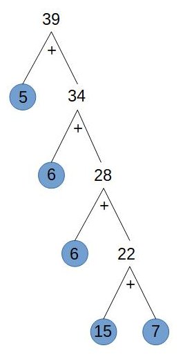
(a) Linear

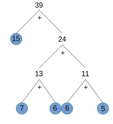
(b) Huffman

Figure 3. Linear and Huffman tree (canonical) summation methods. Our canonical ordering has two main advantages. It reduces the FP summation error in the linear transforms by improving the order of evaluation. It also ensures that we get the same error if we evaluate the same set of points in different orderings; the order of evaluation is determined by the Huffman tree, not by the order in which the points are presented.

We build a Huffman [15] tree using the absolute values of each row, that is used to specify the order of summation. We also use simple heuristics to break ties between coeffients with the same absolute values. A basic principle of accurate FP summation is to try to sum smaller values first, as shown in Figure 3. Our Huffman tree is based purely on the values of the rows of our constant matrices; we build the tree at the algorithm design time, when the input and kernel are unknown. This makes it much easier for us to search empirically for good sets of points because we need only consider their value, not their ordering. In addition this method allows us to use different order of summation for every row of matrices that is not possible to obtain by points permutation.

There are a great deal of different summation methods. They were investigated in detail by Rump ([21], [22]) and Demmel ([8]). They guarantee the accurate or nearly accurate result of dot product computations. However they require additional arithmetic operations either (1) for a compensated summation, or (2) to sort elements before summation, that slow down the convolution computations. These methods trade-off increased accuracy against increased computation cost, which is similar to the mixed-precision method we propose in Section 8.

Our canonical evaluation order is not guaranteed to sum in increasing order of absolute value, because the execution time inputs might contain large or small values. But in practice our canonical ordering does much better than arbitrary orderings. We tested our approach with the setup describe in Section 6. Across a range of convolution sizes using various points we found roughly a $14\%$ improvement in accuracy for $1D$ and $12\%$ for $2D$ compared with the same selection of points in an arbitrary order. All subsequent test results presented in this paper use our Huffman summation for the transforms.

7.2. Point Choice

We empirically evaluated over $40000$ of random selections of values for the points that are used to construct the $G$, $A^{T}$ and $B^{T}$ matrices that are used to perform the linear transforms. We quickly found that it is very easy to find sets of points that cause huge FP errors, and rather more difficult to find better points.

There is no single recognized method for selecting points that minimize the FP error. However, the Chebyshev nodes are known to improve the conditioning of polynomial interpolation [14], which is an important step of Toom-Cook convolution. Results for the FP error of using the Chebyshev nodes can be found in Appendix D. In general, the Chebyshev nodes are orders of magnitude better than typical random point selections.

There is, however, some common wisdom in the literature on another approach to selecting points to reduce the computation in the linear transforms. In general, the points $\{0,-1,1,\infty\}$ are good for reducing these costs, assuming that the code to implement convolution exploits these values. Multiplication by 1 or -1 can simply be skipped, and multiplication by zero allows both the scaling and addition to be skipped. Fortunately, eliminating FP operations also eliminates their associated error, so these points are also suitable to reducing FP error.

Problems start to arise where we need more than just these four basic points. In general, researchers agree that selecting small simple integers and fractions are good choices for reducing the required number of scalings and additions. We also found this type of points to be good for reducing the FP error. But there is no agreed-upon method in the literature for selecting between different values such as $2,-2,\frac{1}{2},-\frac{1}{2},\frac{3}{2},\frac{2}{3}$, etc.

To help us find good sets of these simple values to reduce the FP error, we developed the following rules which act as a heuristic to guide our search. The size of the kernel and output block determine the number of points needed. We start with the basic points $\{0,-1,1,\infty\}$, which work well when four points are needed. We perform our search for sets of good points for output $n$ based on the good sets of points for output $n-1$. We establish a set of potentialy interesting points according to below rules as rationals with numerator in $\{-4,-3,-2,-1,0,1,2,3,4\}$ and denominator in $\{1,2,3,4\}$. This gives us a set $P$ of $23$ possible points.

Our Algorithm

• We start with a set $P_{n-1}$ of $n-1$ good points $p_{1},...,p_{n-1}$

• We construct new sets of points by adding $p_{n}$.
  $P_{n-1}\cup\{p_{n}\}$ $\forall p_{n}$ such that $p_{n}\in P$ and $p_{n}\neq p_{i}$ $\forall i=0,..,n-1.$

• If $n$ is even we construct a new set by dropping $p_{j}$ and adding two new points $p_{k}$ and $-\frac{1}{p_{k}}$.
  As $n$ is even we have at least one point $p_{j}$ without symmetry, that is, $p_{j}\in P_{n-1}$ and $-\frac{1}{p_{j}}\notin P_{n-1}$. We drop the point $p_{j}$ and add instead all pairs $p_{k}$ and $-\frac{1}{p_{k}}$
  $P_{n-1}\setminus\{p_{j}\}\cup\{p_{k},-\frac{1}{p_{k}}\}$ $\forall p_{k}\in P$, $p_{k},-\frac{1}{p_{k}}\neq p_{i}$ $\forall i=0,..,n-1$.

• If there are different sets of points for $1D$ and $2D$ we check both sets for $1D$ and $2D$ in parallel.

The resulting sets of “good” points are presented in Table 2. The basic four points are always $\{0,-1,1,\infty\}$. Table 2 shows that when we add a fifth point, we found empirically that $\frac{1}{2}$ is the best point to add for both 1D and 2D convolution. Occasionally, when moving to the next larger number of points we remove an existing point and add two new ones, such as when we add the eight point for 1D convolution. Note that the FP error versus direct convolution grows rapidly with the number of points. The increased error is due to the algorithm becoming less accurate with more points. The growth in error appears to be roughly exponential in the number of points in practice. However, the growth in error is not smooth (see Figure 5).

Table 2. Example points for Toom-Cook in $FP32$ with kernels of size 3 (for 1D) or $3\times 3$ (for 2D). We start with set of $4$ points $P_{4}=\{0,-1,1,\infty\}$. Then we present the set of points for different cardinality as a additions and/or subtraction of sets of points.

$n$	Points 1D	Error 1D	$n_{o}$	Points 2D	Error 2D	$n_{o}$
0	Direct convolution	1.75E-08	$1$	Direct conv.	4.63E-08	$1\times 1$
4	$P_{4}=\{0,-1,1,\infty\}$	2.45E-08	$2$	$P_{4}$	7.65E-08	$2\times 2$
5	$P_{4}\cup\{\frac{1}{2}\}$	5.19E-08	$3$	$P_{4}\cup\{\frac{1}{2}\}$	2.35E-07	$3\times 3$
6	$P_{4}\cup\{\frac{1}{2},-3\}$	6.92E-08	$4$	$P_{4}\cup\{\frac{1}{2},-2\}$	3.29E-07	$4\times 4$
7	$P_{4}\cup\{\frac{1}{2},-\frac{1}{2},-3\}$	9.35E-08	$5$	$P_{4}\cup\{\frac{1}{2},-2,-\frac{1}{2}\}$	6.81E-07	$5\times 5$
8	$P_{8}=P_{4}\cup\{\frac{1}{2},-\frac{1}{2},2,-2\}$	1.15E-07	$6$	$P_{8}$	8.79E-07	$6\times 6$
9	$P_{8}\cup\{-\frac{1}{4}\}$	2.34E-07	$7$	$P_{8}\cup\{-\frac{1}{4}\}$	3.71E-06	$7\times 7$
10	$P_{10}=P_{8}\cup\{-\frac{1}{4},4\}$	3.46E-07	$8$	$P_{10}$	7.35E-06	$8\times 8$
11	$P_{10}\cup\{\frac{1}{4}\}$	5.91E-07	$9$	$P_{10}\setminus\{0\}\cup\{\frac{3}{4},-\frac{4}{3}\}$	2.2E-05	$9\times 9$
12	$P_{10}\cup\{\frac{3}{4},-\frac{4}{3}\}$	7.51E-07	$10$	$P_{10}\cup\{\frac{3}{4},-\frac{4}{3}\}$	3.22E-05	$10\times 10$
13	$P_{10}\cup\{\frac{3}{4},-\frac{4}{3},\frac{1}{4}\}$	1.32E-06	$11$	$P_{10}\cup\{\frac{3}{4},-\frac{4}{3},\frac{1}{4}\}$	1.09E-04	$11\times 11$
14	$P_{14}=P_{10}\cup\{\frac{1}{4},-\frac{3}{4},\frac{4}{3},-4\}$	1.84E-06	$12$	$P_{14}$	1.99E-04	$12\times 12$
15	$(P_{14}\setminus\{0\})$ $\cup\{\frac{2}{3},-\frac{3}{2}\}$	3.42E-06	$13$	$P_{14}\setminus\{0\}$ $\cup\{\frac{3}{4},-\frac{4}{3}\}$	5.54E-04	$13\times 13$
16	$P_{14}\cup\{\frac{2}{3},-\frac{3}{2}\}$	4.26E-06	$14$	$P_{14}$ $\cup\{\frac{3}{4},-\frac{4}{3}\}$	8.8E-04	$14\times 14$
17	$P_{14}\cup\{\frac{2}{3},-\frac{3}{2},-\frac{2}{3}\}$	1.35E-05	$15$	$P_{14}$ $\cup\{\frac{2}{3},-\frac{3}{2},\frac{3}{2}\}$	1.07E-02	$15\times 15$
18	$P_{14}\cup\{\frac{2}{3},-\frac{3}{2},-\frac{2}{3},\frac{3}{2}\}$	2.24E-05	$16$	$P_{14}\cup\{\frac{2}{3},-\frac{3}{2},-\frac{2}{3},\frac{3}{2}\}$	1.93E-02	$16\times 16$

7.3. Error Growth

If we consider the growth in 1D error from 7 to 8 points, the error grows from $9.35\times 10^{-8}$ to $1.15\times 10^{-7}$, which is a factor of around $1.12\times$. In contrast the growth in error from 8 to 9 points is $1.15\times 10^{-7}$ to $2.34\times 10^{-7}$, which is a factor of $2.03\times$. This is not a coincidence. The empirically good solution that we found when seven points are used for 1D convolution is $\{0,-\frac{1}{2},\frac{1}{2},-1,1,-3,\infty\}$. In contrast when eight points are needed, the good solution is $\{0,-\frac{1}{2},\frac{1}{2},-1,1,-2,2,\infty\}$. Among the eight points there is a symmetry between the four values $\{-\frac{1}{2},\frac{1}{2},-2,2\}$, which are negations and reciprocals of one another. As we discuss in Section 7.4, these symmetries reduce FP error.

In contrast, where 7 points are needed, the points $\{-\frac{1}{2},\frac{1}{2},-3\}$ do not cancel in the same way, and so the error for seven points is larger than a smooth growth in error with points would suggest. Note that the appearance of the point $-3$ as the sixth selected point for 1D convolution was a great surprise to us. However, $-3$ has just two significant binary digits, so there is no representation error of $-3$ in FP, and multiplication by $-3$ causes a very small error. Further, when computing differences between pairs of points for the $B^{T}$ matrix, $-3-(-1)=-2$ and $-3-1=-4$, both of which are even powers of two.

For 2D convolution, small differences mean that $-3$ is very slightly worse than $\frac{1}{2},2$ or $-2$ and is not selected.

Given these trends it is reasonable to ask where are the good trade-offs between computation and error growth. The number of general multiplications is simply the number of points in the convolution algorithm. Using good point selections has no additional cost over bad ones, but greatly reduces the error. Similarly, our Huffman summation reduces the error at no additional computation cost. There is no single best trade-off because it depends on the required accuracy. However, using our point selections and other methods it may be possible to increase the output block size by 1-3 units.

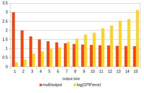
(a) 1D

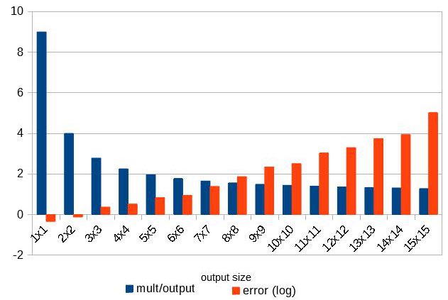
(b) 2D

Figure 4. Number of multiplication and error for single output point for different input block sizes in one- and two-dimensional Toom-Cook convolution

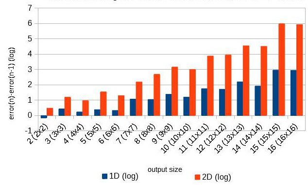
Figure 5. Increasing error in one- and one-dimensional Toom-Cook convolution. The vertical axis show the difference of logarithms from error of convolution computed with $n$ and $n-1$ points, to show error growth.

When we examine the measured errors in Figure 5 we see that even using good point selections the measured error increases roughly exponentially with the size of the convolution. The average measured error grows at a rate that is compatible with the worst-case bound proven in Section 3.

Our analysis in Section 4.4 also suggests that the FP error for 2D convolution grows quadratically more quickly than the error for 1D convolution. This is borne out in Figure 5, where the 2D error as a function of the 1D error is approximately $f(x)=\frac{x^{2}}{2.97}$.

As a further check on the consistency of our measurements, we also implemented a running error analysis for 1D Toom-Cook convolution. Running error analysis [14, p. 65] is an empirical method that computes a partial bound based on actual values alongside the executing algorithm. In our experiments we found that the running error closely matched the exponential rate of growth of the average error, with the running error $4.63\times$ to $7.51\times$ times the average error.

7.4. Discussion of point selection

The point selection affect both components of forward error: conditioning of used matrices and floating point error. The goal of our tests is to find a good balance between them. Based on the our theoretical analysis, literature ([14], [9], [10]) and our empirical experiments those presented in Figure $4$ and many other tests that give us much larger FP error, it is possible to explain why some points are better than others.

One common way to mitigate the Vandermonde matrices ill-conditioning is use Chebyshev nodes. We tried this approach (see Appendix D) but found that this did not perform well. The size of Vandermonde matrices used in DNN convolution is relatively small. The error generated by ill-conditioning grows exponentially. But for the small convolutions in DNNs, the error from ill-conditioning is not so large as to outweigh the error from floating point operation and representation. Chebyshev nodes are mostly irrational, so they can not be represented exactly as FP values. This representation error propagates throughout the algorithm.

In addition, we are interested in the accuracy of discrete convolution. There is a single correct answer (with known degree) to the interpolation in Toom-Cook convolution. If we were computing with infinite precision we could compute the correct polynomial precisely. This is somewhat different to another common use of interpolation, which is to estimate a polynomial where the degree is unknown. The advantages of Chebyshev interpolation points to mitigate Runge’s phenomenon does not help Toom-Cook convolution. We can not ignore conditioning entirely. But our goal is to find a set of points that will minimize both factors: problem conditioning and floating point error.

The four basic points $\{0,-1,1,\infty\}$ are almost always a good choices. In particular $0$ and $\infty$ result in guaranteed zeros in all three matrices $A^{T}$, $G$ and $B^{T}$ which cause no FP error. But we have to explain the point selection for bigger sets. We note that some clear rules for point selection emerge from our empirical study.

Firstly, we should use pairs of points that differ in sign (positive/negative), and pairs of reciprocal points — see Table 2. If we use point $p$ then using $-p$, $\frac{1}{p}$ and $-\frac{1}{p}$ allow us to get better accuracy than introducing other point. Positive/negative pairs of points generate lower elements in matrix $B^{T}$ 1. Looking for the formula of matrix $B^{T}$ elements construction we can noticed that multiplication $(a-p)(a+p)=-p^{2}+0a+a^{2}$ results in zero coefficient of second term. Reciprocal points introduce the coefficient of the first term equal to $1$ in multiplication $(a-p)(a-frac{1}{p}p)=1-\frac{p^{2}+1}{p}a+a^{1}$ that not introduce any additional scalling error. The opposite points are also known to be good for Vandermonde matrices conditioning ([9], [10]).

Secondly, the floating point error boundary depends directly on the values used in operations (see formula 1). That means that we should look for the small values close to one to reduce the error. Putting it together with the previous observation we can say that choosing rational points minimizing numerator and denominator is a good strategy. This approach to points selection has also a positive impact for the floating point error. Assuming that each of kernel and input elements have a similar distribution using scaling factors with similar order of magnitude it is more likely to avoid cancellation error while computing dot product. The interesting point is that for bigger sets this is not always leading rule. We found that $\frac{1}{4}$ together with $(0,-1,1,-1/2,1/2,-2,2)$ works better than $\frac{1}{3}$ for $9$ points (see tables 2, 3). We explain this phenomena later in this section.

Thirdly, representation error of matrices elements have a big impact for the accuracy of the result. As we mentioned below the representation error propagates through all floating point operations and therefore can significantly grow up. This is why the exactly represented points work best in investigated algorithm (see tables 2, 3).

Finally, as we described in subsection (4.2) the error from multiplication while computing the dot product affects on accuracy as well. The elements equal to power of $2$ do not introduce any error from scaling and therefore keep floating point error smaller. This and previous observation explain us why point $\frac{1}{4}4$ is better then $\frac{1}{3}$. The value $\frac{1}{4}$ in contrast to $\frac{1}{3}$ is exactly represented and do not introduce any error from multiplication.

Thus there is not a simple algorithm to choose a set of good points for Winograd algorithm. Our theoretical analysis allow us to identify all components of the error and dramatically narrow the search space. With that knowledge it is possible to check empiricaly which of the narrow sets of points works the best in practice.

8. Mixed-precision pre-/post-processing

We often apply the same kernel to the set of many different inputs. Similarly we often compute convolution with different kernels for the same input data. Thus, the pre-/post processing of each input, kernel and output are done just once, whereas the transformed data is used many times. One way to improve accuracy is to use a mixed-precision algorithm, where the pre-/post processing is done in higher precision, while the inner loops that perform the pairwise multiplication (Hadamard product) are computed in standard precision. This approach lowers the value of machine epsilon $\varepsilon$ for the linear transforms in the error formulsa in Theorems (3) and (8).

Table 3 shows the point selection and measured errors for a mixed-precision Toom-Cook that performs the pre-/processing in FP64 and all other processing in FP32. We found that the mixed precision algorithm reduced the error in both $1D$ and $2D$ by up to around $40\%$ see column ”Ratio” in table (3). The result is that for the same level of error, the mixed-precision algorithm can often allow an ouput size that is one larger. We observe that in most cases the same sets of points worked best for convolution computed in FP32 and in mixed precision. Where there are differences, in most cases this is the result of a slight difference in the order in which points are selected when the number of points is odd. In the mixed-precision rounding errors during the pre-/post processing steps become a little less important because intermediate values are represented in FP64.

The cost of computing in double precision is significant. Modern processors typically use vector arithmetic units, and the throughout of double precision (FP64) is normally just half of single precision (FP32). On graphics processing units (GPUs) the disparity between single and double precision can be much larger. Furthermore, data conversions between single and double precision are normally needed, which further increase the computing cost.

A growing trend in deep neural networks is to store inputs and kernels in FP16 precision in memory, but to compute in FP32. Most Intel and ARM processors do not support FP16 arithmetic. But they provide fast instructions for converting from FP16 values to FP32 to allow FP16 storage and FP32 computation. Many GPUs support native FP16 arithmetic, but it is not commonly used for DNN convolution. FP16 errors accumulate too rapidly for DNN convolution, particularly the errors arising from summation across channels. Recent NVidia GPUs provide co-called tensor cores, which are specifically aimed at storing data in FP16 and computing in FP32. The tensor cores accept FP16 inputs, and compute a multiple-input fused multiply and add operation, which produces a FP32 result. These operations could be used to implement mixed-precision FP16/FP32 linear transforms for Toom-Cook convolution.

Table 3. Example points for Toom-Cook method computations in $FP32$ with transforms in $FP64$ with kernels of size 3 (for 1D) or $3\times 3$ (for 2D). We start with set of $4$ points $P_{4}=\{0,-1,1,\infty\}$. Then we present the set of points for different cardinallity as a additions and/or substractionf of sets of points. The column Ratio present the ratio between the error of convolution computations with transforms in $FP64$ and convolution computations in $FP32$.

$n$	Points 1D	Error 1D	$n_{o}$	Ratio	Points 2D	Error 2D	Ratio
0	Direct convolution	1.75E-08	1	1	Direct convolution	4.63E-08	1
4	$P_{4}=\{0,-1,1,\infty\}$	1.87E-08	2	0.76	$P_{4}$	5.27E-08	0.69
5	$P_{4}\cup\{3\}$	3.66E-08	3	0.71	$P_{4}\cup\{3\}$	1.62E-07	0.69
6	$P_{4}\cup\{3,-\frac{1}{2}\}$	4.41E-08	4	0.64	$P_{4}\cup\{3,-\frac{1}{2}\}$	2.14E-07	0.65
7	$P_{4}\cup\{3,-\frac{1}{2},\frac{1}{2}\}$	6.09E-08	5	0.65	$P_{4}\cup\{3,-\frac{1}{2},\frac{1}{2}\}$	3.69E-07	0.54
8	$P_{8}=P_{4}\cup\{-\frac{1}{2},\frac{1}{2},-2,2\}$	6.97E-08	6	0.61	$P_{8}$	5.18E-07	0.59
9	$P_{8}\cup\{-\frac{1}{4}\}$	1.55E-07	7	0.66	$P_{8}\cup\{4\}$	2.42E-06	0.65
10	$P_{10}=P_{8}\cup\{-\frac{1}{4},4\}$	2.09E-07	8	0.6	$P_{10}$	4.41E-06	0.6
11	$P_{10}\cup\{\frac{1}{4}\}$	3.64E-07	9	0.62	$P_{10}\setminus\{0\}\cup\{\frac{3}{4},-\frac{4}{3}\}$	1.27E-05	0.58
12	$P_{12}=P_{10}\cup\{\frac{3}{4},-\frac{4}{3}\}$	4.50E-07	10	0.6	$P_{12}$	1.89E-05	0.59
13	$P_{12}\cup\{\frac{1}{4}\}$	8.25E-07	11	0.63	$P_{12}\cup\{-4\}$	6.38E-05	0.59
14	$P_{14}=P_{12}\cup\{\frac{1}{4},-4\}$	1.11E-06	12	0.6	$P_{14}$	1.14E-04	0.57
15	$P_{12}\setminus\{0\}\cup\{\frac{2}{3},-\frac{3}{2}\}$	2.17E-06	13	0.63	$P_{12}\setminus\{0\}\cup\{-\frac{3}{4},\frac{4}{3}\}$	3.08E-04	0.56
16	$P_{16}=P_{14}\cup\{\frac{2}{3},-\frac{3}{2}\}$	2.78E-06	14	0.65	$P^{\prime}_{16}=P_{14}\cup\{-\frac{3}{4},\frac{4}{3}\}$	4.95E-04	0.56
17	$P_{16}\cup\{-\frac{2}{3}\}$	8.43E-06	15	0.62	$P^{\prime}_{16}\cup\{\frac{3}{2}\}$	5.93E-03	0.55
18	$P_{18}=P_{16}\cup\{-\frac{2}{3},\frac{3}{2}\}$	1.39E-05	16	0.62	$P_{18}$	1.04E-02	0.54

9. Multiple channels

The proposed techniques up to this point of the paper have been for simple 1D or 2D convolution with a size $3$ or $3\times 3$ matrix respectively. However, an important feature of convolution in deep neural networks is multiple channels. Convolution inputs and kernels in many of the best known DNNs, such as GoogLeNet [24] or ResNet [13] typically have something between 3 and 1024 channels. However, the number of channels is a parameter selected by the designer of the neural network, and there is no upper limit on the number of channels used.

When performing convolution, a separate 1D or 2D convolution is performed at each channel, and then the results of each separate convolution is summed with the corresponding values in the other channels see figure 1. The obvious way to implement summation across channels is to perform the complete convolution separately on each channel, and sum the results. However, this would require that the post-processing linear transform is applied on each channel, which is a relatively expensive operation. Lavin and Gray [18] observed that the items can be summed before the linear transform, so that the post-processing step need be applied only to the sum. Therefore, in order to perform convolution over multiple channels we have to sum up the results of pairwise multiplication (Hadamard product) before we apply the transposition represented by $A^{T}$ matrix. The convolution is computed according the following formulas:

$$A^{T}(\sum_{channels}(Gh\odot B^{T}x))$$

$$A^{T}(\sum_{channels}(GHG^{T}\odot B^{T}XB))A$$

As a result, the FP error from DNN convolution is not just the error of the 1D or 2D convolution, but also the error from summing across channels. This is important for two reasons. First, if using Toom-Cook convolution increases the numerical error. The impact of summation over channels in error formulas (4.6) and (4.6) is represented by $\lambda$.

Second, there are well-known techniques for reducing the error from summation. If we reduce the error of summation, this may offset some part of the loss of accuracy arising from Toom-Cook convolution.

In section 8 we proposed a mixed precision algorithm that does pre-/post-processing in higher precision. However, this is not a suitable approach to increase the accuracy of the summation across channels. The summation across channels is in the inner-most loop of DNN convolution, so we cannot afford to double its cost. We instead propose using the well-known pairwise summation algorithm [17] for summation across channels.

When summing $n$ FP inputs, the worst-case error from simply accumulating to a single variable is $O(n)$. In contrast, the pairwise summation algorithm has a worst-case error of just $O(\log_{2}n)$ [17]. Given our existing error bound for Toom-Cook convolution with multiple channels, we can formulate the effect of using pairwise summation rather than linear summation.

Corollary 3.

The error for 1D convolution based on theorems (3) and (8), using linear summation across channels is:

(12) $$\|\hat{s}-s\|_{1}\leq\|A^{T}\|_{1}\thinspace\|G\|_{F}\thinspace\|B^{T}\|_{F}\thinspace\|h\|_{F}\thinspace\|x\|_{F}\left(\alpha^{(n)}+\beta^{(n)}+\gamma^{(n_{h})}+C\right)\varepsilon+O(\varepsilon^{2})$$

For pairwise summation across channels, the corresponding error is:

(13) $$\begin{split}&\|\hat{s}-s\|_{1}\leq\\ &\leq\|A^{T}\|_{1}\thinspace\|G\|_{F}\thinspace\|B^{T}\|_{F}\thinspace\|h\|_{2}\thinspace\|x\|_{2}\left(\alpha^{(n)}+\beta^{(n)}+\gamma^{(n_{h})}+\lfloor log(C)\rfloor+2\right)\varepsilon+O(\varepsilon^{2})\end{split}$$

As we can observe comparing formulas (12) and (13) we have smaller overall error when we use the pairwise summation over channels than for linear summation.

Tables 4, 5, 6, 7 present measured errors for Toom-Cook convolution with just a single channel, with 32 channels, and with 64 channels. We see that the error per output value for 64 input channels is much larger than the error for just a single input channel. But the error is around 2–20 times larger, not 64 times larger. The reason is that when these values are summed, some of the errors cancel one another.

Our results presented in tables 4, 5 show that pairwise summation can reduce the total FP error by around 20%–40%. Similar tests presented in tables 6,7 show that when pairwise summation across channels is used with mixed-precision transforms, the improvement compared to mixed-precision transforms alone is 25%-45%. Using both proposed methods: mixed precision and pairwise summation (8) give us an improvement in accuracy of around $50\%$ in both one- and two-dimensional computations.

Table 4. Toom-Cook over multiple channels in $FP32$ — error per single output point for 1 dimension convolution. Columns ”ratio in $\%$” present the ratio of error per single output point get with pairwise summation and error per single output point with liner summation in $\%$.

Out	1	32	32 channels	ratio	64	64 channels	ratio
size	channel	channels	pairwise sum	in $\%$	channels	pairwise sum	in $\%$
1	1.75E-08	2.74E-07	1.90E-07	$69\%$	5.12E-07	2.87E-07	56$\%$
2	2.45E-08	3.80E-07	2.71E-07	$71\%$	7.03E-07	4.00E-07	57$\%$
3	5.19E-08	7.08E-07	5.11E-07	$72\%$	1.28E-06	7.59E-07	59$\%$
4	6.92E-08	8.35E-07	6.17E-07	$74\%$	1.48E-06	9.18E-07	62$\%$
5	9.35E-08	1.09E-06	8.35E-07	$77\%$	2.00E-06	1.24E-06	62$\%$
6	1.15E-07	1.31E-06	9.79E-07	$75\%$	2.34E-06	1.47E-06	63$\%$
7	2.34E-07	2.90E-06	2.16E-06	$74\%$	5.21E-06	3.20E-06	61$\%$

Table 5. Toom-Cook over multiple channels in $FP32$ - error per single output point for two-dimensional convolution. Columns ”ratio in $\%$” present the ratio of error per single output point get with pairwise summation and error per single output point with linear summation in $\%$.

Out	1	32	32 channels	ratio	64	64 channels	ratio
size	channel	channels	pairwise sum	in $\%$	channels	pairwise sum	in $\%$
$1\times 1$	4.63E-08	5.25E-07	3.95E-07	$75\%$	9.44E-07	5.83E-07	62$\%$
$2\times 2$	7.65E-08	9.05E-07	6.47E-07	$71\%$	1.65E-06	9.59E-07	58$\%$
$3\times 3$	2.35E-07	2.87E-06	2.09E-06	$73\%$	5.33E-06	3.11E-06	58$\%$
$4\times 4$	3.29E-07	3.60E-06	2.70E-06	$75\%$	6.56E-06	3.98E-06	61$\%$
$5\times 5$	6.81E-07	7.78E-06	5.71E-06	$73\%$	1.41E-05	8.57E-06	61$\%$
$6\times 6$	8.79E-07	9.48E-06	7.12E-06	$75\%$	1.71E-05	1.04E-05	61$\%$
$7\times 7$	2.43E-06	4.66E-05	3.41E-05	$73\%$	8.41E-05	5.09E-05	61$\%$

Table 6. Toom-Cook computation in $FP32$ with transforms in $FP64$- error per single output point for 1 dimension convolution. Columns ”ratio in $\%$” present the ratio of error per single output point get with pairwise summation and error per single output point with liner summation in $\%$.

Out	1	32	32 channels	ratio	64	64 channels	ratio
size	channel	channels	pairwise sum	in $\%$	channels	pairwise sum	in $\%$
1	1.75E-08	2.73E-07	1.90E-07	$70\%$	5.15E-07	2.88E-07	$56\%$
2	1.87E-08	3.60E-07	2.31E-07	$64\%$	6.73E-07	3.58E-07	$53\%$
3	3.66E-08	6.50E-07	4.39E-07	$68\%$	1.20E-06	6.72E-07	$56\%$
4	4.41E-08	7.45E-07	5.16E-07	$69\%$	1.41E-06	7.86E-07	$56\%$
5	6.09E-08	1.00E-06	6.98E-07	$70\%$	1.92E-06	1.06E-06	$55\%$
6	6.97E-08	1.17E-06	7.90E-07	$68\%$	2.18E-06	1.20E-06	55$\%$
7	1.55E-07	2.60E-06	1.80E-06	$69\%$	4.91E-06	2.75E-06	56$\%$

Table 7. Toom-Cook computation in $FP32$ with transforms in $FP64$- error per single output point for two-dimensional convolution. Columns ”ratio in $\%$” present the ratio of error per single output point get with pairwise summation and error per single output point with liner summation in $\%$.

Out	1	32	32 channels	ratio	64	64 channels	ratio
size	channel	channels	pairwise sum	in $\%$	channels	pairwise sum	in $\%$
$1\times 1$	4.63E-08	5.25E-07	3.95E-07	$75\%$	9.48E-07	5.85E-07	$62\%$
$2\times 2$	5.27E-08	8.51E-07	5.54E-07	$65\%$	1.59E-06	8.48E-07	$53\%$
$3\times 3$	1.62E-07	2.70E-06	1.80E-06	$67\%$	5.13E-06	2.75E-06	$54\%$
$4\times 4$	2.14E-07	3.60E-06	2.36E-06	$66\%$	6.68E-06	3.61E-06	$54\%$
$5\times 5$	3.69E-07	6.06E-06	4.07E-06	$67\%$	1.14E-05	6.17E-06	$54\%$
$6\times 6$	5.18E-07	8.48E-06	5.64E-06	$67\%$	1.59E-05	8.53E-06	$54\%$
$7\times 7$	3.39E-06	4.21E-05	2.91E-05	$69\%$	8.03E-05	4.34E-05	$54\%$

Table 8. Ratio of Toom-Cook in $FP32$ with linear summation over the channels and in mixed precision with pairwise summation over the channels - error for single output point in $1$ and $2$ dimensions.

Output size	32	64	Output size	32	64
1D	channels	channels	2D	channels	channels
1	$69\%$	$56\%$	$1\times 1$	$75\%$	$62\%$
2	$61\%$	$51\%$	$2\times 2$	$61\%$	$51\%$
3	$62\%$	$53\%$	$3\times 3$	$63\%$	$52\%$
4	$62\%$	$53\%$	$4\times 4$	$66\%$	$55\%$
5	$65\%$	$53\%$	$5\times 5$	$52\%$	$44\%$
6	$60\%$	$51\%$	$6\times 6$	$59\%$	$50\%$
7	$62\%$	$53\%$	$7\times 7$	$62\%$	$52\%$

10. Related work

Lavin and Gray [18] wrote the seminal paper on applying Winograd convolution to deep neural networks. They showed how to apply 2D versions of these algorithms to DNN convolution with multiple input and output channels, and how to amortize the cost of pre-/post-processing over many convolutions. Although they used the Toom-Cook method to generate their core convolution algorithms, they refered to it as Winograd convolution, and that has become the accepted term in the DNN literature.

By far the closest existing work to ours is from Vincent et al. [28]. They propose to scale convolution matrices to reduce the condition number of the Vandermonde matrices. They demonstrate that this approach can reduce the error number in exactly one case: convolving a $5\times 5$ kernel to create a $9\times 9$ output block. Further they showed that this improved matrix could be used to successfully for training a DNN. However, they did not provide a method for choosing good scaling factors. Our approach to reducing FP error is equally empirical, but we focus on constructing good convolution matrices rather than improving them after construction. We measured the error for our $5\times 5$, $9\times 9$ (with 13 points) convolution matrices and compared it with Vincent et al.’s solution. We found that our convolution matrices yield an error that is around 45% lower (better) than Vincent et al.’s.

The idea of applying the Toom-Cook algorithm to compute convolution was investigated and in great detail by Shmuel Winograd [30]. He focused on the low complexity of Toom-Cook convolution, and proved that it is optimal with respect to the number of general multiplications. Winograd developed his own method of generating short convolution algorithms based on the Chinese remainder theorem. Winograd’s method can create a much larger set of algorithms than Toom-Cook, including algorithms that are not optimal with respect to general mutliplications.

To the best of our knowledge, this paper is the first that presents a theoretical analysis of the numerical error of Toom-Cook convolution. We demonstrate that the algorithm is unstable because the properties of algorithm parameters matrices we use ($G$, $B^{T}$, $A^{T}$). We formulate the boundaries of the FP errors for one- and two-dimensional kernels and inputs so we can resonable choose what we should focus on to improve the accuracy. We formulated the error bounds for Toom-Cook convolution using similar techniqes to those used for another bilinear problem: the fast matrix multiplication, error estimation by Bini and Lotti [3], Demmel et al. [7] and [1]. We show that algorithm is unstable and how the error depends on each component.

As we can see from our errors formulation, the stability of the Toom-Cook convolution depends directly on the values of the matrices $G$, $A^{T}$ and $B^{T}$ not only on input and kernel values and sizes. While it has been empirically observed and theoreticaly proven that the condition number of square Vandermonde matrices containing real (not complex) points increases exponentially, to our knowledge there is no theoretically-sound method for choosing the best points. There are some more specific boudaries for particular sets of points, i.e. harmonic, equidistance, positive, in the range $(-1,1)$ [14] and complex points [19]. The way we choose points in our tests allow us to obtain sets of good points for specific input and kernel sizes, but points were find to be good empirically do not follow any of these simple patters. In general, minimizing the numerator and denominator works well, but it is not always the best approach. The FP representation [11] [14] and symmetry of reciprocal and inverse points [5] [10] matters as well.

In our search for the best points, we studied a wide range of literature on the conditiining of Vandermonde matrices dating from the last $40+$ years [19] [10] [9] [14] and Toom-Cook algorithm [5] [23]. We took under consideration all theoretical results we found while developing our strategy for finding good points. Since there is not any clear pattern of points to choose, the lack of theoretical background on Vandermonde inverse matrix norm did not allow us to present any more advanced analysis.

Some work on Toom-Cook optimality was done by M. Bodrato [5]. He focused on the optimality of this algorithm applied to the polynomial multiplication problem, as measured by the number of operations required. Improving the floating numerical accuracy of the result was not a goal of Bodrato’s work, and no data data is provided of the effect of the proposed techniques on numerical accuracy. In contrast, our work studied Toom-Cook algorithm application for the DNN convolution problem; we consider a much bigger variety of input sizes and additional factors that have an impact on accuracy like FP precision. However, as we have shown, reducing the number of operations required for the pre-/post-processing steps can improve numerical accuracy. Just as we found that symmetric points can improve numerical accuracy, Bodrato found that such points could reduce the number of required operations.

Note that our focus is on reducing Toom-Cook FP error to allow larger outblock block sizes and thus fewer general multiplications. However, error analysis might also be used for other purposes such as identifying when the training error has become smaller than the FP error, and that therefore training can be terminated early. We leave such additional uses of error analysis to future work.

11. Conclusions

We present an analysis of 1D and 2D Toom-Cook convolution with multiple channels for DNN convolution. We identify and formalize the error terms for Toom-Cook convolution, and prove that the error bound grows at least exponentially with the size of the convolution. This result is supported by an analysis of conditioning, which shows that the condition number of the convolution with respect to the norm grows exponentially with convolution size.

We formally analyse the error bound for the “modified” Toom-Cook algorithm, and prove that the error is close to that of the non-modified algorithm operating on an input one element smaller. We observe empirically that using modified version reduces the error by $20\%$ to over $70\%$, with no additional computation cost.

We observe that the order of point selection impacts the accuracy of the algorithm. We propose a canonical evaluation order based on Huffman trees. This fixes the order of evaluation, and empirically reduces the error by a further 12%-14% in addition to the improvement from using the modified algorithm, again with no additional computation cost.

There is no existing, widely accepted strategy for selecting points. We observe that for DNNs there is a relatively small number of important sizes, and we search empirically for good point selections for those sizes. We identify four key criteria for good point selections: (1) few significant mantissa bits, (2) positive/negative point symmetry, (3) reciprocal point symmetry, and (4) subtractions of points leading to few significant mantissa bits. For important convolution sizes for DNNs, our empirically selected points yield much better accuracy than the Chebyshev nodes. The Chebyshev nodes fail to meet our criteria (1), (3) and (4) which makes them relatively poor choices for the small convolutions found in DNNs.

We also proposed a mixed precision approach where the transforms are computed in double precision, while the remaining inner loops are computed in $FP32$. We found that perfoming pre/post processing transforms in $FP64$ decreases error typically by around one third in our experiments. We also empirically investigated summation across channels using pairwise summation and found that this reduces the error by around 20% to 50%. Unlike the other methods we investigated, mixed precision transforms and pairwise summation impose an additional computation cost.

Using our point selections and techniques for improving FP accuracy, we can reduce the error between $2\times$ and orders of magnitude, when compared with the Chebyshev nodes. Each approximately $2\times$ reduction in the error allows the output block size dimension to be increased by around one. Whereas current implementations of Winograd convolution for DNNs typically use output block sizes of $2\times 2$ or $3\times 3$, our methods allow larger block sizes, with a resulting reduction in arithmetic operations (see Table 1). This will allow faster DNN training and inference, which is particularly valuable for resource-constrained mobile and embedded systems.

APPENDIX

Appendix A Estimate of norm and conditioning

In this appendix, we provide some estimates of the norm and conditioning of the product $W(h,x)=A^{T}\left(Gh\odot B^{T}x\right)$ in terms of an expression involving only the matrices $A$, $G$, and $B$ and one involving $x$ and $h$. To do this, we reformulate this Hadamard product using a special product of two matrice called the Khatri-Rao product, which can be thought of as a specific block analog of the Hadamard product; see [12].

Definition 1.

Let $C,F$ be $m\times n$ block matrices with the structure

$$C=\left(C_{ij}\right)_{ij}\qquad\mbox{and}\qquad F=\left(F_{ij}\right)_{ij}$$

with block sizes $C_{ij},F_{ij}\in\mathbb{R}^{s_{i}\times s_{j}}$. The Khatri-Rao product is the blockwise Kronecker product defined by $C\otimes_{KR}F=\left(C_{ij}\otimes F_{ij}\right)_{ij}$.

The Khatri-Rao product can be used to express the Hadamard product $Gh\odot B^{T}x$ as a matrix-vector product, whereby we use block both matrices by row. That means the $C\otimes_{KR}F$ here denotes the matrix whose rows consist of the Kronecker products of the rows of $C$ and $F$.

Theorem 6.

The Hadamard product $Gh\odot B^{T}x$ admits the expression

$$Gh\odot B^{T}x=\left(B^{T}\otimes_{KR}G\right)\cdot\left(x\otimes h\right).$$

Proof.

Let

$$G=\begin{bmatrix}g_{1}^{T}\\ g_{2}^{T}\\ \vdots\\ g_{nx}^{T}\end{bmatrix}\qquad\mbox{and}\qquad B^{T}=\begin{bmatrix}b_{1}^{T}\\ b_{2}^{T}\\ \vdots\\ b_{nx}^{T}\end{bmatrix}$$

with $b_{i}^{T}=\begin{bmatrix}b_{i1}&b_{i2}&\cdots&b_{i,n_{x}}\end{bmatrix}$. Then the $i$th entry of $B^{T}h$ is $b_{i}^{T}x=\sum_{j=1}^{n_{x}}b_{ij}x_{j}$. and the $i$th entry of $Gh\odot B^{T}x$ can thus be written as

$$g_{i}^{T}h\cdot b_{i}^{T}x=g_{i}^{T}h\cdot\sum_{j=1}^{n_{x}}b_{ij}x_{j}=\sum_{j=1}^{n_{x}}b_{ij}g_{i}^{T}\left(x_{j}h\right),$$

which can be written as the vector dot product

$$g_{i}^{T}h\cdot b_{i}^{T}x=\begin{bmatrix}b_{i1}g_{i}^{T}&b_{i2}g_{i}^{T}&\cdots&b_{i,n_{x}}g_{i}^{T}\end{bmatrix}\begin{bmatrix}x_{1}h\\ x_{2}h\\ \vdots\\ x_{n_{x}}h\end{bmatrix}=\left(b_{i}^{T}\otimes g_{i}^{T}\right)\left(x\otimes h\right).$$

This proves the result. ∎

We now calculate the condition number of $W(h,x)$. Recall that for a continuous function $f(x)$ and a given vector norm $\left\|\cdot\right\|$, we can express the relative condition number in terms of the induced operator norm of its Jacobian $J_{f}(x)$

$$\kappa(x)=\dfrac{\left\|J_{f}(x)\right\|\cdot\left\|x\right\|}{\left\|f(x)\right\|};$$

see, e.g., [27]. We can write the composition $W(h,x)=W(y)$ where $y:=y(h,x)=x\otimes h$. Then we can use the chain rule to express the Jacobian of $W(h,x)$ as

$$J_{w}(h,x)=A^{T}\left(B^{T}\otimes_{KR}G\right)J_{y}(x,h),$$

where $J_{y}(h,x)$ is the Jacobian of $y(h,x)$. Thus the condition number for $W(h,x)$ satisfies

(14) $$\kappa_{W}(h,x)=\dfrac{\left\|A^{T}\left(B^{T}\otimes_{KR}G\right)J_{y}(x,h)\right\|\cdot\left\|x\otimes h\right\|}{\left\|A^{T}\left(B^{T}\otimes_{KR}G\right)\cdot\left(x\otimes h\right)\right\|}.$$

We can then get an upper bound estimate for this condition number. We begin by introducing some terminology. If $C\in\mathbb{R}^{m\times m}$ is nonsingular, then it is a well-known result that the condition number $\kappa_{2}(C)$ with respect to $\left\|\cdot\right\|_{2}$ satisfies $\kappa_{2}(C)=\dfrac{\sigma_{max}(C)}{\sigma_{min}(C)}$, where $\sigma_{max}(C),\sigma_{min}(C)>0$ are, respectively, the largest and smallest singular value of $C$, which are guaranteed by the nonsingularity of $C$ to be nonzero.

Theorem 7.

The condition number $\kappa_{W}(h,x)$ with respect to $\left\|\cdot\right\|_{1}$ admits the upper bound estimate

$$\kappa_{W}(h,x)\leq\sqrt{n_{o}nn_{h}}\max\left\{\left\|x\right\|_{1},\left\|h\right\|_{1}\right\}\kappa_{2}\left(A^{T}\left(B^{T}\otimes_{KR}G\right)\right).$$

Proof.

We must get appropriate lower bound estimates for the denominator of $\kappa_{w}(h,x)$ in order to get an upper bound estimate of the whole expression. First, observe that we have from vector norm equivalence $\left\|A^{T}\left(B^{T}\otimes_{KR}G\right)\cdot\left(x\otimes h\right)\right\|_{1}\geq\left\|A^{T}\left(B^{T}\otimes_{KR}G\right)\cdot\left(x\otimes h\right)\right\|_{2}$. Next, we take advantage of the fact that in theory, the three matrices are square, nonsingular Vandermonde matrices. This allows us to unambgiuously construct a chain of inequalities,

$$\left\|A^{T}\left(B^{T}\otimes_{KR}G\right)\cdot\left(x\otimes h\right)\right\|_{2} =\left\|A^{T}\left(B^{T}\otimes_{KR}G\right)\cdot\dfrac{x\otimes h}{\left\|x\otimes h\right\|_{2}}\right\|_{2}\left\|x\otimes h\right\|_{2}$$

$$\geq\min_{y\in\mathbf{R}^{nn_{h}}\atop\left\|y\right\|_{2}=1}\left\|A^{T}\left(B^{T}\otimes_{KR}G\right)\cdot y\right\|_{2}\left\|x\otimes h\right\|_{2}$$

$$\geq\sigma_{min}\left(A^{T}\left(B^{T}\otimes_{KR}G\right)\right)\left\|x\otimes h\right\|_{2}.$$

Applying this to (14)

(15) $$\kappa_{W}(h,x)\leq\dfrac{\left\|A^{T}\left(B^{T}\otimes_{KR}G\right)J_{y}(x,h)\right\|_{1}\cdot\left\|x\otimes h\right\|_{1}}{\sigma_{min}\left(A^{T}\left(B^{T}\otimes_{KR}G\right)\right)\left\|x\otimes h\right\|_{2}}.$$

Using vector norm equivalence, we can estimate $\left\|x\otimes h\right\|_{1}\leq\sqrt{nn_{h}}\left\|x\otimes h\right\|_{2}$. We have the induced matrix norm inequality

$$\left\|A^{T}\left(B^{T}\otimes_{KR}G\right)J_{y}(x,h)\right\|_{1}\leq\left\|A^{T}\left(B^{T}\otimes_{KR}G\right)\right\|_{1}\left\|J_{y}(x,h)\right\|_{1}.$$

Writing out $J_{y}(x,h)$, one observes that $\left\|J_{y}(x,h)\right\|_{1}=\max\left\{\left\|x\right\|_{1},\left\|h\right\|_{1}\right\}$. Furthermore, for $C\in\mathbb{R}^{m_{1}\times m_{2}}$, we have the matrix norm equivalence $\dfrac{1}{\sqrt{m_{1}}}\left\|C\right\|_{1}\leq\left\|C\right\|_{2}\leq\sqrt{m_{2}}\left\|C\right\|_{1}$. Applied in this setting yields

$$\left\|A^{T}\left(B^{T}\otimes_{KR}G\right)\right\|_{1}\leq\sqrt{n_{o}}\left\|A^{T}\left(B^{T}\otimes_{KR}G\right)\right\|_{2}=\sqrt{n_{o}}\,\sigma_{max}\left(A^{T}\left(B^{T}\otimes_{KR}G\right)\right).$$

Substituting into (15) yields the result after some simplificaton. ∎

What this demonstrates is that in the one-dimensional case, conditioning of the underlying problem, i.e., the relative condition number of the convolution with respect to $\left\|\cdot\right\|_{1}$, has a bound which grows worse exponentially as the size of the Vandermonde matrices grows. This is not surprising in light of the error analysis shown earlier. However, we also see that the condition number has an upper bound depending on $\left\|x\right\|_{1}$ and $\left\|h\right\|_{1}$, meaning that we cannot rule out that the convolution may exhibit poorer conditioning in the case that $x$ and $h$ are pathologically large.

Appendix B Proof of the theorem of two-dimensional Toom-Cook error bounds

B.1. Two-dimensional Toom-Cook convolution error

Theorem 8.

Error for two-dimensional Toom-Cook convolution computation satisfies the componentwise bound equal to:

(16) $$\begin{split}|\hat{S}-S|&\leq\\ \leq&|A^{T}|\left(|G||H||G^{T}|\odot|B^{T}||X||B|\right)|A|\left(2\alpha^{(n)}+2\beta^{(n)}+2\gamma^{(n_{h})}+1\right)\varepsilon+\O(\varepsilon^{2})\\ \end{split}$$

Error for two-dimensional Toom-Cook convolution computation satisfies the normwise bound equal to:

(17) $$\begin{split}\|\hat{S}-S\|_{1}&\leq\\ &\leq\|A^{T}\|_{1}\thinspace\|G\|_{F}\thinspace\|H\|_{F}\thinspace\|G^{T}\|_{F}\thinspace\|B^{T}\|_{F}\thinspace\|X\|_{F}\thinspace\|B\|_{F}\thinspace\|A\|_{1}\thinspace R\varepsilon+O(\varepsilon^{2})\;\;\;\;\;\;\;\;\;\\ \mathrm{where}\;R&=2\alpha^{(n)}+2\beta^{(n)}+2\gamma^{(n_{h})}+1\;\;\;\;\;\;\;\;\;\;\;\;\;\;\;\;\;\;\;\;\;\;\;\;\end{split}$$

If we assume the same method of summation while matrix and transpose matrix multiplication.
Where $\alpha^{(n)}$, $\beta^{(n)}$, $\gamma^{(n_{h})}$ represents the error from multiplication by matrices $A^{T}$, $B^{T}$ and $G$ respectively.

Proof.

In computing two-dimensional convolution we use the feature of Kronecker product that means $vec(MXM^{T})=(M\otimes M)vec(X)$. Notice that despite the both formulas are mathematically equivalent the result in FP arithmetic could be different because of more multiplication operations while computing $vec(MXM^{T})$ than for $(M\otimes M)vec(X)$.
We have

$$|fl(fl(A)Xfl(A^{T}))|=|A|\thinspace|X|\thinspace|A^{T}|2\alpha^{(n)}\varepsilon+O(\varepsilon^{2})$$

. Let put component function

$$S=g(H,X)=g_{3}(g_{2}(g_{1}^{H}(H),g_{1}^{X}(X)))$$

$g(H,X):\mathbb{R}^{n_{h}\times n_{h}}\times\mathbb{R}^{n\times n}\rightarrow\mathbb{R}^{n_{o}\times n_{o}}$, $\;\;g(H,X)=A^{T}\left(GHG^{T}\odot B^{T}XB\right)A$,
$g_{3}:\mathbb{R}^{n\times n}\rightarrow\mathbb{R}^{n_{o}\times n_{o}}$, $\;\;g_{3}(M)=A^{T}m$,
$g_{2}:\mathbb{R}^{n\times n}\times\mathbb{R}^{n\times n}\rightarrow\mathbb{R}^{n\times n}$, $\;\;g_{2}(M,N)=M\odot N$,
$g_{1}:\mathbb{R}^{n_{h}\times n_{h}}\rightarrow\mathbb{R}^{n\times n}$, $\;\;g_{1}^{H}(M)=GMG^{T}$ and $g_{1}^{X}:\mathbb{R}^{n\times n}\rightarrow\mathbb{R}^{n\times n}$.
Similarly as for one-dimensional convolution we have:

$$|vec(\hat{S})-vec(S)|\leq|J_{3}|\thinspace|J_{2}|\thinspace|\Delta b_{2}|+|J_{2}|\thinspace|\Delta b_{3}|+|\Delta b_{4}|=$$

$$=|A^{T}\otimes A^{T}|\left[Diag((|B^{T}|\otimes|B^{T}|)vec(|X|)),Diag((|G|\otimes|G|)vec(|H|))\right]|$$

$$|\left[\begin{array}[]{l}\left(|G|\otimes|G|\right)vec\left(|H|\right)2\gamma^{(n_{h})}\varepsilon+O(\varepsilon^{2})\\ \left(|B^{T}|\otimes|B^{T}|)vec(|X|\right)|2\beta^{(n)}\varepsilon+O(\varepsilon^{2})\end{array}\right]|+$$

$$+\left(|A^{T}|\otimes|A^{T}|\right)\left(\left(|G|\otimes|G|\right)vec\left(|H|\right)\odot\left(|B^{T}|\otimes|B^{T}|\right)vec\left(|X|\right)\right)\varepsilon+O(\varepsilon^{2})+$$

$$\left(|A^{T}|\otimes|A^{T}|\right)\left(\left(|G|\otimes|G|\right)vec\left(|H|\right)\odot\left(|B^{T}|\otimes|B^{T}|\right)vec\left(|X|\right)\right)2\alpha^{(n)}\varepsilon+O(\varepsilon^{2})=$$

$$=\left(|A^{T}|\otimes|A^{T}|\right)\left(\left(|G|\otimes|G|\right)vec\left(|H|\right)\odot\left(|B^{T}|\otimes|B^{T}|\right)vec\left(|X|\right)\right)\left(2\gamma^{(n_{h})}+2\beta^{(n)}\right)\varepsilon\thinspace+$$

$$+\left(|A^{T}|\otimes|A^{T}|\right)\left(\left(|G|\otimes|G|\right)vec\left(|H|\right)\odot\left(|B^{T}|\otimes|B^{T}|\right)vec\left(|X|\right)\right)\left(2\alpha^{(n)}+1\right)\varepsilon+O(\varepsilon^{2})=$$

$$=\left(|A^{T}|\otimes|A^{T}|\right)\left(|G|\otimes|G|\right)vec\left(|H|\right)\odot\left(|B^{T}|\otimes|B^{T}|\right)vec\left(|X|\right)|\thinspace R\varepsilon+\thinspace O(\varepsilon^{2})=$$

$$R=2\gamma^{(n_{h})}+2\beta^{(n)}+2\alpha^{(n)}+1$$

Changing vectors again to matrices we obtain:

$$|\hat{S}-S|\leq|A^{T}|\left(|G|\thinspace|H|\thinspace|G^{T}|\odot|B^{T}|\thinspace|X|\thinspace|B|\right)|A|\left(2\alpha^{(n)}+2\beta^{(n)}+2\gamma^{(n_{h})}+1\right)\varepsilon+O(\varepsilon^{2})$$

We do the normwise error estimationin in the same way as for one-dimensional convolution, as the matrix consistency and Buniakowski-Schwartz inequality holds both for vectors and matrices.

$$\|\hat{S}-S\|_{1}\leq\|A^{T}\left(GHG^{T}\odot B^{T}XB\right)A\left(2\alpha^{(n)}+2\beta^{(n)}+2\gamma^{(n_{h})}+1\right)\varepsilon+O(\varepsilon^{2})\|\leq$$

$$\leq\|A^{T}\left(GHG^{T}\odot B^{T}XB\right)A\|_{1}\left(2\alpha^{(n)}+2\beta^{(n)}+2\gamma^{(n_{h})}+1\right)\varepsilon+O(\varepsilon^{2})$$

From norm $\|\cdot\|_{1}$ consistency:

$$\|\hat{S}-S\|_{1}\leq\|A^{T}\|_{1}\|\left(GHG^{T}\right)\odot\left(B^{T}XB\right)\|_{1}\|A\|_{1}\left(2\alpha^{(n)}+2\beta^{(n)}+2\gamma^{(n_{h})}+1\right)\varepsilon+O(\varepsilon^{2})$$

Applying Buniakowski-Schwartz inequality for Hadamard product:

$$\|\hat{S}-S\|_{1}\leq\|A^{T}\|_{1}\thinspace\|GHG^{T}\|_{F}\thinspace\|B^{T}XB)\|_{F}\thinspace\|A\|_{1}\left(2\alpha^{(n)}+2\beta^{(n)}+2\gamma^{(n_{h})}+1\right)\varepsilon+O(\varepsilon^{2})$$

Finally from norm equivalency:

$$\|\hat{S}-S\|_{1}\leq\|A^{T}\|_{1}\thinspace\|G\|_{F}\thinspace\|H\|_{F}\thinspace\|G^{T}\|_{F}\thinspace\|B^{T}\|_{F}\thinspace\|X\|_{F}\thinspace\|B\|_{F}\thinspace\|A\|_{1}\thinspace R\varepsilon+O(\varepsilon^{2})$$

$$R=2\alpha^{(n)}+2\beta^{(n)}+2\gamma^{(n_{h})}+1$$

∎

Appendix C Modified Toom-Cook convolution error analysis

Theorem 9.

The componentwise error for one-dimensional modified Toom-Cook for $q$th element of output is bounded by:

(18) $$\begin{split}&|\hat{s}^{m(n)}_{q}-s^{m(n)}_{q}|=\\ &=|{A^{T}_{q:}}^{(n-1)}|\thinspace\left(|G^{(n-1)}|\thinspace|h|\odot|B^{(n-1)T}|\thinspace|x^{(n-1)}|\right)\left(\gamma^{(n_{h})}+\beta^{(n-1)}+\alpha^{(n-1)}+1\right)\varepsilon+O(\varepsilon^{2})\\ &\mathrm{for}\;q=1,..,n_{o}-1\\ &\\ &|{\hat{s}_{n_{o}}}^{(m(n))}-s^{m(n)}_{n_{o}}|\leq\\ &\leq|{A^{T}_{q:}}^{(n-1)}|\left(|G^{(n-1)}|\thinspace|h|\odot|B^{(n-1)T}|\thinspace|x^{(n-1)}|+|h_{n_{h}}|\thinspace|{B_{n:}}^{m(n)T}|\thinspace|x|\right)\\ &\;\;\;\;\;\;\;\;\;\left(max\left\{\left(\gamma^{(n_{h})}+\beta^{(n-1)}+\alpha^{(n-1)}+1\right),\left(\beta+1\right)\right\}+1\right)\varepsilon+O(\varepsilon^{2})\\ &\mathrm{for}\;q=n_{o}\end{split}$$

Proof.

We denote matrices constructed for Toom-Cook algorithm of input size $n$ as $G^{(n)}$, $A^{(n)T}$ and $B^{(n)T}$ and for modified Toom-Cook algorithm of input size $n$ as $G^{m(n)}$, $A^{m(n)T}$ and $B^{m(n)T}$.

As we can see from the modified Toom-Cook algorithm definition we solve the problem of size $n$ by solving problem of size $n-1$ by Toom-Cook algorithm and proper modify the last element of output. Thus is obvious that error boundary of the first $n_{o}-1$ output points in modified Toom-Cook convolution is equal to the boundary of Toom-Cook convolution for input size $n-1$. The computation of the last $n_{o}$th output point include two parts: we compute the partial result using Toom-Cook convolution for input $n-1$ and add the missing value. ${s_{n_{o}}}^{m(n)}={s^{(n-1)}_{n_{o}}}+h_{n_{h}}B^{m(n)_{n:}}x$ So:

$$|{\hat{s}_{n_{o}}}^{m(n)}-s_{n_{o}}^{m(n)}|\leq$$

$$|{s_{n_{o}}}^{(n-1)}|\left(\gamma^{(n_{h})}+\beta^{(n-1)}+\alpha^{(n-1)}+1\right)\varepsilon+O(\varepsilon^{2})+|h_{n_{h}}|\thinspace|{B_{n:}}^{m(n)T}|\thinspace|x|(\beta^{(n)}+1)\varepsilon+O(\varepsilon^{2})=$$

$$=\left(|{s_{n_{o}}}^{(n-1)}|+|h_{n_{h}}|\thinspace|{B_{n:}}^{m(n)T}||x|\right)max\left\{\gamma^{(n_{h})}+\beta^{(n-1)}+\alpha^{(n-1)}+1,\beta^{n}+1\right\}\varepsilon+O(\varepsilon^{2})$$

∎

For DNN convolution the kernel size $n_{h}$ is almost always greater than or equal to $3$ and $n_{h}\leq n$. If we compute the convolution then from dot product error analysis we know that $\gamma^{(n_{h})}\geq n_{h}-1$, $\beta^{(n-1)}\geq n-2$ and $\alpha^{(n-1)}\geq n-2$. In this case $\gamma^{(n_{h})}+\beta^{(n-1)}+\alpha^{(n-1)}+1\geq n_{h}+2n-4$, while $\beta^{(n)}+1\leq n+2$. When $n_{h}\geq 3$ the maximum in formula 18 is always equal to $\gamma^{(n_{h})}+\beta^{(n-1)}+\alpha^{(n-1)}+1$. So we can formulate following corollary:

Corollary 4.

If we use the kernel size $n_{h}\geq 3$ computing for 1D convolution using modified Toom-Cook algorithm then the componentwise error for last output element is bounded as follows:

(19) $$\begin{split}&|{\hat{s}_{n_{o}}}^{(m(n))}-s^{m(n)}_{n_{o}}|\leq\\ &\leq|{A^{T}_{q:}}^{(n-1)}|\left(|G^{(n-1)}|\thinspace|h|\odot|B^{(n-1)T}|\thinspace|x^{(n-1)}|+|h_{n_{h}}|\thinspace|{B_{n:}}^{m(n)T}|\thinspace|x|\right)R\varepsilon+O(\varepsilon^{2})\end{split}$$

where $R=\left(\gamma^{(n_{h})}+\beta^{(n-1)}+\alpha^{(n-1)}+1\right)$

Assuming any elements in matrices $G^{m(n)}$, $B^{m(n)T}$ and $A^{m(n)T}$ and linear summation while compute the dot product we have following boundaries:

Corollary 5.

$$\begin{split}&|{\hat{s}_{n_{o}}}^{(m(n))}-s^{m(n)}_{n_{o}}|\leq\\ &\leq(|{A^{T}_{q:}}^{(n-1)}|(|G^{(n-1)}||h|\odot|B^{(n-1)T}||x^{(n-1)}|+|h_{n_{h}}||{B_{n:}}^{m(n)T}||x|)(n_{h}+2n+2)\varepsilon+O(\varepsilon^{2})\end{split}$$

Appendix D Tests results for Chebyshev nodes

The table below presented the error of convolution computations for different sizes with Chebyshev points and the points we found the best. The column ”Ratio” presents how many times the error for Chebyshev points is bigger then for points we found.

	1D	1D	1D	2D	2D	2D
n	Our points	Chebyshev	Ratio	Our points	Chebyshev	Ratio
4	2.49E-08	3.51E-08	1.41	7.65E-08	1.01E-07	1.32
5	5.21E-08	5.535E-08	1.06	2.46E-07	2.12E-07	8.62
6	7.32E-08	1.04E-07	1.42	3.49E-07	5.65E-07	1.62
7	1.00E-07	1.68E-07	1.68	7.11E-07	1.70E-06	2.39
8	1.23E-07	3.78E-07	3.07	9.21E-07	6.50E-06	7.06
9	2.59E-07	6.76E-07	2.61	4.07E-06	2.59E-05	6.36
10	3.87E-07	1.48E-06	3.82	8.23E-06	1.09E-04	1.32E+01
11	6.62E-07	3.18E-06	4.80	2.53E-05	4.84E-04	1.91E+01
12	8.42E-07	7.46E-06	8.86	3.67E-05	2.18E-03	5.94E+01
13	1.56E-06	1.53E-05	9.81	1.24E-04	1.00E-02	8.06E+01
14	2.10E-06	3.21E-05	15.29	2.32E-04	4.72E-02	2.03E+02
15	3.91E-06	7.12E-05	18.21	6.35E-04	2.31E-01	3.64E+02
16	5.06E-06	1.56E-04	30.83	1.04E-03	1.10	1.06E+03
17	1.68E-05	3.53E-04	21.01	1.31E-02	5.43	4.15E+02
18	2.36E-05	8.03E-04	34.03	0.24E-02	26.91	1.12E+04

Table 9. Error for one- and two-dimensional convolution for Chebyshev points and points we found. Column ”Ratio” present how many times the error for Chebyshev points is bigger then for points we found.

References

- [1] Grey Ballard, Austin R. Benson, Alex Druinsky, Benjamin Lipshitz, and Oded Schwartz, Improving the numerical stability of fast matrix multiplication, SIAM Journal on Matrix Analysis and Applications 37 (2016), no. 4, 1382–1418.
- [2] Norman L. Biggs, Discrete mathematics, 2nd. ed., Oxford University Press, New York, NY, USA, 2002.
- [3] Dario Bini and Grazia Lotti, Stability of fast algorithms for matrix multiplication, Numerische Mathematik 36 (1980), no. 1, 63–72.
- [4] Richard E. Blahut, Fast algorithms for signal processing, Cambridge University Press, New York, NY, USA, 2010.
- [5] Marco Bodrato, Towards optimal toom-cook multiplication for univariate and multivariate polynomials in characteristic 2 and 0, Arithmetic of Finite Fields (Berlin, Heidelberg) (Sunar B. Carlet C., ed.), Lecture Notes in Computer Science, vol. 4547, Springer-Verlag, 2007, pp. 116–133.
- [6] Stephen A. Cook, On the minimum computation time of functions, Ph.D. thesis, Harvard University, Cambridge, Mass., 1966.
- [7] James Demmel, Ioana Dumitriu, Olga Holtz, and Robert Kleinberg, Fast matrix multiplication is stable, Numerische Mathematik 106 (2007), no. 2, 199–224.
- [8] James Demmel and Yozo Hida, Accurate and efficient floating point summation, SIAM Journal on Scientific Computing 25 (2004), 1214–1248.
- [9] Walter Gautschi, Norm estimates for inverses of Vandermonde matrices, Numerische Mathematik 23 (1974), 337–347.
- [10] by same author, How (un)stable are Vandermonde systems?, Asymptotic and Computational Analysis 124 (1990), 193–210.
- [11] David Goldberg, What every computer scientist should know about floating-point arithmetic, ACM Computing Surveys 23 (1991), no. 1, 5–48.
- [12] Gene H. Golub and Charles F. Van Loan, Matrix Computations, fourth ed., Johns Hopkins Studies in the Mathematical Sciences, Johns Hopkins University Press, Baltimore, MD, 2013. MR 3024913
- [13] Kaiming He, Xiangyu Zhang, Shaoqing Ren, and Jian Sun, Deep residual learning for image recognition, 2016 IEEE Conference on Computer Vision and Pattern Recognition (CVPR), June 2016, pp. 770–778.
- [14] Nicholas J. Higham, Accuracy and stability of numerical algorithms, 2nd. ed., SIAM Publications, Philadelphia, PA, 2002.
- [15] David Huffman, A method for the construction of minimum-redundancy codes, Proceedings of the IRE 40 (1952), no. 9, 1098–1101.
- [16] William Kahan, The improbability of probabilistic error analyses for numerical computations, Slides from Statistics Colloqium, University of California, Berkeley, February 1996.
- [17] Donald E. Knuth, The art of computer programming, Addison-Wesley, USA, 1998.
- [18] Andrew Lavin and Scott Gray, Fast algorithms for convolutional neural networks, 2016 IEEE Conference on Computer Vision and Pattern Recognition (CVPR) (Las Vegas, Nevada), IEEE, 2016, pp. 4013–4021.
- [19] Victor Y. Pan, How bad are vandermonde matrices?, SIAM J. Matrix Analysis Applications 37 (2016), no. 2, 676–694.
- [20] Keshab K. Parhi, Vlsi digital signal processing systems: Design and implementation, John Wiley and Sons, New York, 2007.
- [21] Siegfried M. Rump, Takeshi Ogita, and Shin’ichi Oishi, Accurate floating-point summation part I: faithful rounding, SIAM Journal on Scientific Computing 31 (2008), no. 1, 189–224.
- [22] by same author, Accurate floating-point summation part II: sign, k-fold faithful and rounding to nearest, SIAM Journal on Scientific Computing 31 (2008), no. 2, 1269–1302.
- [23] Ivan W. Selesnick and C. Sidney Burrus, Extending Winograd’s small convolution algorithm to longer lengths, 1994 IEEE International Symposium on Circuits and Systems, ISCAS (London, England), IEEE, May 1994, pp. 449–452.
- [24] Christian Szegedy, Wei Liu, Yangqing Jia, Pierre Sermanet, Scott Reed, Dragomir Anguelov, Dumitru Erhan, Vincent Vanhoucke, and Andrew Rabinovich, Going deeper with convolutions, Proceedings of the 2015 IEEE Conference on Computer Vision and Pattern Recognition (CVPR), June 2015, pp. 1–9.
- [25] Richard Tolimieri, Myoung An, and Chao Lu, Algorithms for discrete fourier transform and convolution, 2nd. ed., Springer-Verlag, New York, NY, USA, 1997.
- [26] Andrei L. Toom, The complexity of a scheme of functional elements realizing multiplication of integers, Soviet Mathematics – Doklady 3 (1963), 714–716.
- [27] Lloyd N. Trefethen and David Bau, Numerical linear algebra, SIAM, Philadelphia, 1997.
- [28] Kevin Vincent, Kevin Stephano, Michael Frumkin, Boris Ginsburg, and Julien Demouth, On improving the numerical stability of winograd convolutions, Proceedings of the 5th International Conference on Learning Representations (Toulon, France), 2017, https://openreview.net/forum?id=H1ZaRZVKg, p. 4.
- [29] James H. Wilkinson, Rounding errors in algebraic processes, Dover Publications, New York, NY, USA, 1994.
- [30] Shmuel Winograd, Arithmetic complexity computations, SIAM Publications, Bristol, England, 1980.
- [31] by same author, Signal processing and complexity of computation, IEEE International Conference on Acoustics, Speech, and Signal Processing, ICASSP (Denver, Colorado), IEEE, April 1980, pp. 94–101.