Abstract

In this paper, we revisit our model–independent methods developed for reconstructing properties of Weakly Interacting Massive Particles (WIMPs) by using measured recoil energies from direct Dark Matter detection experiments directly and take into account more realistically non–negligible threshold energy. All expressions for reconstructing the mass and the (ratios between the) spin–independent and the spin–dependent WIMP–nucleon couplings have been modified. We focus on low–mass ($m_{\chi}\>\raisebox{-3.01385pt}{$\stackrel{{\scriptstyle\textstyle<}}{{\sim}}$}\>~{}\!15$ GeV) WIMPs and present the numerical results obtained by Monte Carlo simulations. Constraints caused by non–negligible threshold energy and technical treatments for improving reconstruction results will also be discussed.

1 Introduction

So far Weakly Interacting Massive Particles (WIMPs) arising in several extensions of the Standard Model of particle physics are still one of the leading candidates for cosmological Dark Matter. In the last three decades, a large number of experiments have been built and are being planned to search for different WIMP candidates by direct detection of scattering recoil energies of ambient WIMPs off target nuclei in low–background underground laboratory detectors (see Refs. [1, 2, 3, 4, 5, 6, 7, 8, 9, 10, 11, 12, 13, 14, 15, 16]).

Using data from these direct Dark Matter detection experiments to reconstruct, e.g., the mass and different couplings on nucleons is essential for understanding the nature of WIMPs and identifying them among new particles produced at colliders. Different methods have been purposed for reconstructing the WIMP mass $m_{\chi}$ [17, 18, 19, 20] and spin–independent (SI)/spin–dependent (SD) WIMP–nucleon cross sections $\sigma_{\chi{\rm(p,n)}}^{\rm SI,SD}$ [21, 22]. Recently, several applications of the maximum likelihood and Bayesian analyses have been developed, which treat the WIMP mass and different WIMP–nucleon couplings as well as the Solar and Earth’s orbital velocities in the Galactic reference frame as fitting parameters simultaneously (see works by, e.g., Y. Akrami et al. [23, 24], M. Pato et al. [25, 26], C. Arina et al. [27, 28, 29, 30], D. G. Cerde$\rm\tilde{n}$o et al. [31, 32, 33] and e.g. [34, 35, 36, 37]). Furthermore, while some authors focus on studying effects of and/or constraints caused by uncertainties on the velocity and density distributions of Galactic Dark Matter [38, 39, 40, 41], some model–independent methods have also been developed by P. J. Fox et al. [42, 43, 44], E. Del Nobile et al. [45, 46, 47, 48, 49, 50], B. Feldstein and F. Kahlhoefer [51, 52, 53], G. B. Gelmini et al. [54, 55, 56, 57] and e.g. [58, 59].

Besides these works, we started also in 2003 to study methods for reconstructing properties of WIMP particles by using (not a fitted recoil spectrum but) the measured recoil energies directly as model–independently as possible. As the first step, in Ref. [60] we introduced an exponential ansatz for reconstructing the measured recoil spectrum and in turn for reconstructing the (moments of the) time–averaged one–dimensional velocity distribution of halo WIMPs. This analysis requires no prior knowledge about the local WIMP density nor a WIMP scattering cross section on nucleus, the only required information is the mass of incident WIMPs. However, with a few hundreds or even thousands recorded events, only a few ($<$ 10) reconstructed points of the WIMP velocity distribution with pretty large statistical uncertainties could be obtained. In order to provide more detailed information about the WIMP velocity distribution as well as the characteristic Solar and Earth’s Galactic velocities, we introduced therefore later the Bayesian analysis into our reconstruction procedure [61] for fitting a functional form of the one–dimensional velocity distribution as well as for determining concretely, e.g., the position of the peak of the fitted velocity distribution function and the values of the characteristic Solar and Earth’s Galactic velocities. Moreover, based on the reconstruction of the moments of the one–dimensional WIMP velocity distribution function and the combinations of two or more experimental data sets with different target nuclei, we developed further the methods for model–independently determining the WIMP mass $m_{\chi}$ [62], the (squared) SI scalar WIMP–proton coupling $|f_{\rm p}|^{2}$ [63] as well as the ratios of the SD axial–vector (to the SI scalar) WIMP–nucleon couplings/cross sections $a_{\rm n}/a_{\rm p}$ and $\sigma_{\chi({\rm p,n})}^{\rm SD}/\sigma_{\chi{\rm p}}^{\rm SI}$ [64].

In these earlier works – both of the theoretical derivations and numerical simulations – the minimal experimental cut–off energies of data sets to be analyzed are often assumed to be negligible. For experiments with heavy target nuclei, e.g. Ge or Xe, and once WIMPs are heavy ($\>\raisebox{-3.01385pt}{$\stackrel{{\scriptstyle\textstyle>}}{{\sim}}$}\>~{}100$ GeV), the systematic bias caused by this assumption could be neglected, compared with the pretty large statistical uncertainties. However, once WIMPs are light ($\>\raisebox{-3.01385pt}{$\stackrel{{\scriptstyle\textstyle<}}{{\sim}}$}\>~{}50$ GeV) and a light target nucleus, e.g. Si or Ar, is used, effects of non–negligible threshold energy has to be considered seriously and the expressions for the reconstructions of different WIMP properties and estimates of the statistical uncertainties would need to be modified properly. Meanwhile, some experimental collaborations have developed several detector techniques with different materials for searching for low–mass WIMPs. For instance, the CRESST experiment with their $\rm Al_{2}O_{3}$ and $\rm CaWO_{4}$ detectors [65, 66, 67, 68, 69], the CoGeNT and CDEX experiments with p–type point–contact Ge detectors [70, 71, 72, 73, 74, 75], and the newest generation of the CDMS, the SuperCDMS, experiment with also Ge detectors [76, 77, 78, 79]. Recently, the PICO Collaboration with their PICO-2L $\rm C_{3}F_{8}$ bubble chamber [80, 81] and the DarkSide Collaboration with their DarkSide-50 Ar detector [82] have also announced the sensitivity on detecting low–mass WIMPs.

Therefore, as a supplement of our earlier works, in [83] we have considered the needed modification of the normalization constant of the reconstructed one–dimensional WIMP velocity distribution function caused by non–negligible experimental threshold energy. And, in this paper, we revisit further our methods for the reconstructions of the WIMP mass as well as the (ratios between the) SI (scalar) and the SD (axial–vector) WIMP–nucleon couplings/cross sections by taking into account non–negligible experimental threshold energies of the analyzed data sets. All expressions for the reconstructions of $m_{\chi}$ and (the ratios of) $\sigma_{\chi{\rm(p,n)}}^{\rm SI,SD}$ have been checked and modified properly. We focus on effects of non–negligible threshold energy on the reconstructed WIMP properties for WIMP masses of $m_{\chi}\>\raisebox{-3.01385pt}{$\stackrel{{\scriptstyle\textstyle<}}{{\sim}}$}\>$ 15 GeV.

The remainder of this paper is organized as follows. In Sec. 2, we first review our model–independent procedures for reconstructing different WIMP properties and modify our expressions. Then, in Sec. 3, we present numerical results of the reconstructed WIMP properties by using the modified expressions and discuss effects of non–negligible threshold energy for light WIMPs. We conclude in Sec. 4 and give some technical details for our analysis in Appendix.

2 Formalism

In this section, we first review briefly the modification of the normalization constant of the reconstructed one–dimensional WIMP velocity distribution. Then we derive the corresponding modifications of the expressions for our model–independent reconstructions of different WIMP properties.

2.1 Modification of the normalization constant of the one–dimensional velocity distribution function

The general expression for the differential event rate for elastic WIMP–nucleus scattering with both of the SI and the SD cross sections can be given by [6, 64]:

$$\frac{dR}{dQ}=\frac{\rho_{0}}{2m_{\chi}m_{\rm r,N}^{2}}\bigg{[}\sigma_{0}^{\rm SI}F_{\rm SI}^{2}(Q)+\sigma_{0}^{\rm SD}F_{\rm SD}^{2}(Q)\bigg{]}\int_{v_{\rm min}}^{\infty}\left[\frac{f_{1}(v)}{v}\right]dv~{}\!.$$ (1)

Here $R$ is the direct detection event rate, i.e. the number of events per unit time and unit mass of detector material, $Q$ is the energy deposited in the detector, $\rho_{0}$ is the WIMP density near the Earth, $f_{1}(v)$ is the one–dimensional velocity distribution function of the WIMPs impinging on the detector, $v$ is the absolute value of the WIMP velocity in the laboratory frame. $\sigma_{0}^{\rm(SI,SD)}$ are the SI/SD total cross sections ignoring the form factor suppression and $F_{\rm(SI,SD)}(Q)$ indicate the elastic nuclear form factors corresponding to the SI/SD WIMP interactions, respectively. The reduced mass $m_{\rm r,N}$ is defined by $m_{\rm r,N}\equiv m_{\chi}m_{\rm N}/\left(m_{\chi}+m_{\rm N}\right)$, where $m_{\chi}$ is the WIMP mass and $m_{\rm N}$ that of the target nucleus. Finally, $v_{\rm min}$ is the minimal incoming velocity of incident WIMPs that can deposit the energy $Q$ in the detector:

$$v_{\rm min}(Q)=\alpha\sqrt{Q}$$ (2)

with the transformation constant $\alpha\equiv\sqrt{m_{\rm N}/2m_{\rm r,N}^{2}}$.

As the first step of our model–independent methods for reconstructing the one–dimensional velocity distribution as well as other particle properties of halo WIMPs, the entire experimental possible energy range between the minimal and maximal cut–offs $Q_{\rm min}$ and $Q_{\rm max}$ of the analyzed data set needs to be divided into $B$ bins with central points $Q_{n}$ and widths $b_{n}$ [60]:

$${\textstyle Q_{n}-\frac{b_{n}}{2}}\leq Q_{n,i}\leq{\textstyle Q_{n}+\frac{b_{n}}{2}}~{}\!,~{}~{}~{}~{}~{}~{}~{}~{}~{}~{}~{}~{}i=1,~{}2,~{}\cdots,~{}N_{n},~{}n=1,~{}2,~{}\cdots,~{}B,$$ (4)

where $Q_{n,i}$ denotes the measured recoil energy in the $n$th $Q-$bin and in each bin, $N_{n}$ events will be recorded. Since the recoil spectrum $dR/dQ$ is expected to be approximately exponential, in order to approximate the spectrum in a rather wider range, the following exponential ansatz for the measured recoil spectrum (before normalized by the exposure ${\cal E}$) in the $n$th bin has been introduced [60]:

$$\left(\frac{dR}{dQ}\right)_{{\rm expt},~{}\!n}\equiv\left(\frac{dR}{dQ}\right)_{{\rm expt},~{}\!Q\simeq Q_{n}}\equiv r_{n}~{}\!e^{k_{n}(Q-Q_{s,n})}~{}\!.$$ (5)

Here $r_{n}=N_{n}/b_{n}$ is the standard estimator for $(dR/dQ)_{\rm expt}$ at $Q=Q_{n}$, $k_{n}$ is the logarithmic slope of the recoil spectrum in the $n$th $Q-$bin, which can be computed numerically from the average value of the measured recoil energies in this bin [60]:

$$\overline{Q-Q_{n}}|_{n}\equiv\frac{1}{N_{n}}\sum_{i=1}^{N_{n}}\left(Q_{n,i}-Q_{n}\right)=\left(\frac{b_{n}}{2}\right)\coth\left(\frac{b_{n}k_{n}}{2}\right)-\frac{1}{k_{n}}~{}\!.$$ (6)

Then the shifted point $Q_{s,n}$ in the ansatz (5), can be estimated by [60]

$$Q_{s,n}=Q_{n}+\frac{1}{k_{n}}\ln\left[\frac{\sinh(b_{n}k_{n}/2)}{b_{n}k_{n}/2}\right]~{}\!.$$ (7)

In Ref. [60], we derived that the functional form of the one–dimensional velocity distribution function can be given by the recoil spectrum as

$$f_{1}(v)={\cal N}\left\{-2Q\cdot\frac{d}{dQ}\left[\frac{1}{F^{2}(Q)}\left(\frac{dR}{dQ}\right)\right]\right\}_{Q=v^{2}/\alpha^{2}}~{}\!.$$ (8)

By substituting the ansatz (5) into this functional form of $f_{1}(v)$ and letting $Q=Q_{s,n}$, the reconstructed velocity distribution at points $v_{s,n}=\alpha\sqrt{Q_{s,n}}$ can thus be estimated by [60]

$$f_{1,{\rm rec}}(v_{s,n})={\cal N}\Bigg{[}\frac{2Q_{s,n}r_{n}}{F^{2}(Q_{s,n})}\Bigg{]}\left[\frac{d}{dQ}\ln F^{2}(Q)\bigg{|}_{Q=Q_{s,n}}-k_{n}\right]~{}\!.$$ (9)

In Ref. [83], we considered further a minimal cut–off of the velocity distribution due to non–zero experimental threshold energy, $v_{\rm min}(Q_{\rm min})=\alpha\sqrt{Q_{\rm min}}\equiv v_{\rm min}^{\ast}$, and introduced a model–independent trianglar estimator for the area under $f_{1}(v)$ in the range of $0\leq v\leq v_{\rm min}^{\ast}$. Then the normalization condition for the reconstructed velocity distribution function can be approximated by [83]

$$\int_{0}^{\infty}f_{1}(v)~{}\!dv \simeq f_{1,{\rm rec}}(v_{\rm min}^{\ast})\cdot\frac{v_{\rm min}^{\ast}}{2}+{\cal N}\int_{Q_{\rm min}}^{Q_{\rm max}^{\ast}}\left\{-2Q\cdot\frac{d}{dQ}\left[\frac{1}{F^{2}(Q)}\left(\frac{dR}{dQ}\right)\right]\right\}\left(\frac{\alpha}{2\sqrt{Q}}\right)dQ$$ (10)

$$\simeq f_{1,{\rm rec}}(v_{\rm min}^{\ast})\cdot\frac{\alpha\sqrt{Q_{\rm min}}}{2}+{\cal N}\left(\frac{\alpha}{2}\right)\left[\frac{2Q_{\rm min}^{1/2}r(Q_{\rm min})}{F^{2}(Q_{\rm min})}+I_{0}(Q_{\rm min},Q_{\rm max}^{\ast})\right]$$

$$= 1~{}\!.$$

Here we have defined

$$r(Q_{\rm min})\equiv\left(\frac{dR}{dQ}\right)_{{\rm expt},~{}\!Q=Q_{\rm min}}=r_{1}~{}\!e^{k_{1}(Q_{\rm min}-Q_{s,1})}~{}\!,$$ (11)

with $r_{1}=N_{1}/b_{1}$, is an estimated value of the measured recoil spectrum $(dR/dQ)_{\rm expt}$ at $Q=Q_{\rm min}$, and $I_{n}(Q_{\rm min},Q_{\rm max}^{\ast})$ can be estimated through the sum running over all events in the data set:

$$I_{n}(Q_{\rm min},Q_{\rm max}^{\ast})\equiv\int_{Q_{\rm min}}^{Q_{\rm max}^{\ast}}Q^{(n-1)/2}\left[\frac{1}{F^{2}(Q)}\left(\frac{dR}{dQ}\right)\right]dQ\to\sum_{a}\frac{Q_{a}^{(n-1)/2}}{F^{2}(Q_{a})}~{}\!.$$ (12)

Note that, since the WIMP–nucleus scattering spectrum is expected to be exponential, the term of $\left(dR/dQ\right)_{{\rm expt},~{}\!Q=Q_{\rm max}^{\ast}}$ appearing in the second term of the second line in Eq. (10) has been ignored. Moreover, by substituting Eq. (5) into Eq. (8) and setting $Q=Q_{\rm min}$, one can have

$$f_{1,{\rm rec}}(v_{\rm min}^{\ast}) = {\cal N}\Bigg{[}\frac{2Q_{\rm min}r(Q_{\rm min})}{F^{2}(Q_{\rm min})}\Bigg{]}\left[\frac{d}{dQ}\ln F^{2}(Q)\bigg{|}_{Q=Q_{\rm min}}-k_{1}\right]~{}\!.$$ (13)

Hence, a model–independent approximation for the modified normalization constant ${\cal N}$ which can be estimated directly from the data is given by [83]

$${\cal N} = \frac{2}{\alpha}\left\{\Bigg{[}\frac{2Q_{\rm min}^{1/2}r(Q_{\rm min})}{F^{2}(Q_{\rm min})}\Bigg{]}\bigg{[}K_{1}(Q_{\rm min})~{}\!Q_{\rm min}+1\bigg{]}+I_{0}(Q_{\rm min},Q_{\rm max}^{\ast})\right\}^{-1}~{}\!,$$ (14)

where we have defined

$$K_{n}(Q)\equiv\frac{d}{dQ}\ln F^{2}(Q)-k_{n}~{}\!.$$ (15)

2.2 Reconstructions of the WIMP mass and the SI WIMP–nucleon coupling

Now we revisit our model–independent procedures for the determination of the WIMP mass $m_{\chi}$ and the (squared) SI scalar WIMP–nucleon coupling $|f_{\rm p}|^{2}$. The modified expressions corresponding to the modification of the normalization constant ${\cal N}$ given in Eq. (14) will be derived here. For more detailed discussions about these methods, please see Refs. [62, 63].

From the functional form (8) of $f_{1}(v)$, one can find that

$$\int_{v_{\rm min}^{\ast}}^{v_{\rm max}}v^{n}f_{1}(v)~{}\!dv\simeq{\cal N}\left(\frac{\alpha^{n+1}}{2}\right)\left[\frac{2Q_{\rm min}^{(n+1)/2}r(Q_{\rm min})}{F^{2}(Q_{\rm min})}+(n+1)I_{n}(Q_{\rm min},Q_{\rm max}^{\ast})\right]~{}\!,$$ (16)

where a term $2Q_{\rm max}^{\ast~{}\!(n+1)/2}\left(dR/dQ\right)_{{\rm expt},~{}\!Q=Q_{\rm max}^{\ast}}/F^{2}(Q_{\rm max}^{\ast})$ has been ignored${}^{,~{}\!}$. Then, similar to the calculation of the normalization condition given in Eq. (10), the moments of the one–dimensional WIMP velocity distribution function can be approximated by

$$\langle{\textstyle{v^{n}}}\rangle \equiv \int_{0}^{\infty}v^{n}f_{1}(v)~{}\!dv$$ (17)

$$\simeq f_{1,{\rm rec}}(v_{\rm min}^{\ast})\cdot\frac{(v_{\rm min}^{\ast})^{n+1}}{2}+\int_{v_{\rm min}^{\ast}}^{v_{\rm max}}v^{n}f_{1}(v)~{}\!dv$$

$$\simeq {\cal N}\left(\frac{\alpha^{n+1}}{2}\right)\left\{\Bigg{[}\frac{2Q_{\rm min}^{(n+1)/2}r(Q_{\rm min})}{F^{2}(Q_{\rm min})}\Bigg{]}\bigg{[}K_{1}(Q_{\rm min})~{}\!Q_{\rm min}+1\bigg{]}+(n+1)I_{n}(Q_{\rm min},Q_{\rm max}^{\ast})\right\}$$

$$= \alpha^{n}\left[\frac{2Q_{\rm min}^{(n+1)/2}r^{\ast}(Q_{\rm min})/F^{2}(Q_{\rm min})+(n+1)I_{n}(Q_{\rm min},Q_{\rm max}^{\ast})}{2Q_{\rm min}^{1/2}r^{\ast}(Q_{\rm min})/F^{2}(Q_{\rm min})+I_{0}(Q_{\rm min},Q_{\rm max}^{\ast})}\right]~{}\!.$$

Here the modified normalization constant ${\cal N}$ given in Eq. (14) has been used and we have defined

$$r^{\ast}(Q_{\rm min}) \equiv r(Q_{\rm min})\Big{[}K_{1}(Q_{\rm min})~{}\!Q_{\rm min}+1\Big{]}~{}\!.$$ (18)

In our earlier work on the determination of the WIMP mass $m_{\chi}$, it has already been found that by requiring that the values of a given moment of $f_{1}(v)$ estimated by Eq. (17) from two experiments with different target nuclei, $X$ and $Y$, agree, $m_{\chi}$ appearing in the prefactor $\alpha^{n}$ on the right–hand side of Eq. (17) can be solved analytically as [62]

$$\left.m_{\chi}\right|_{\left<{v^{n}}\right>}=\frac{\sqrt{m_{X}m_{Y}}-m_{X}({\cal R}_{n,X}/{\cal R}_{n,Y})}{{\cal R}_{n,X}/{\cal R}_{n,Y}-\sqrt{m_{X}/m_{Y}}}~{}\!,$$ (19)

with ${\cal R}_{n,(X,Y)}$ now modified directly as

$${\cal R}_{n,X}\equiv\left[\frac{2Q_{{\rm min},X}^{(n+1)/2}r_{X}^{\ast}(Q_{{\rm min},X})/F_{X}^{2}(Q_{{\rm min},X})+(n+1)I_{n,X}}{2Q_{{\rm min},X}^{1/2}r_{X}^{\ast}(Q_{{\rm min},X})/F_{X}^{2}(Q_{{\rm min},X})+I_{0,X}}\right]^{1/n}~{}\!,$$ (20)

and ${\cal R}_{n,Y}$ can be defined analogously. Here $n\neq 0$, $m_{(X,Y)}$ and $F_{(X,Y)}(Q)$ are the masses and the form factors of the nucleus $X$ and $Y$, respectively, and $r_{(X,Y)}^{\ast}(Q_{{\rm min},(X,Y)})$ refer to the counting rates (modified by Eq. (18)) for the target $X$ and $Y$ at the relatively lowest recoil energies included in the analysis.

On the other hand, assuming the SI scalar WIMP interaction dominates, the zero–momentum–transfer cross section in Eq. (1) can be expressed as [6]

$$\sigma_{0}^{\rm SI}=\left(\frac{4}{\pi}\right)m_{\rm r,N}^{2}\Big{[}Zf_{\rm p}+(A-Z)f_{\rm n}\Big{]}^{2}\simeq A^{2}\left(\frac{m_{\rm r,N}}{m_{\rm r,p}}\right)^{2}\sigma_{\chi{\rm p}}^{\rm SI}~{}\!.$$ (21)

Here $Z$ is the atomic number of the target nucleus, i.e. the number of protons, $A$ is the atomic mass number, $A-Z$ is then the number of neutrons, $f_{\rm(p,n)}$ are the effective scalar couplings of WIMPs on protons p and on neutrons n, respectively; the theoretical prediction that the scalar couplings on protons and on neutrons are approximately equal: $f_{\rm n}\simeq f_{\rm p}$ has been adopted, the tiny mass difference between a proton and a neutron has been neglected, and

$$\sigma_{\chi{\rm p}}^{\rm SI}=\left(\frac{4}{\pi}\right)m_{\rm r,p}^{2}|f_{\rm p}|^{2}$$ (22)

is the SI WIMP–nucleon cross section. Now, by applying Eq. (16) with $n=-1$ and substituting the expression (21) for $\sigma_{0}^{\rm SI}$ into Eq. (1), we can have

$$\left(\frac{dR}{dQ}\right)_{{\rm expt},~{}\!Q=Q_{\rm min}}={\cal E}A^{2}\left(\frac{\rho_{0}}{2m_{\chi}}\right)\left[\left(\frac{4}{\pi}\right)|f_{\rm p}|^{2}\right]F_{\rm SI}^{2}(Q_{\rm min})\left\{{\cal N}\left[\frac{r(Q_{\rm min})}{F_{\rm SI}^{2}(Q_{\rm min})}\right]\right\}~{}\!.$$ (23)

It can therefore obtain that [63]

$$|f_{\rm p}|^{2}=\frac{1}{\rho_{0}}\left(\frac{\pi}{4\sqrt{2}}\right)\left(\frac{1}{{\cal E}A^{2}\sqrt{m_{\rm N}}}\right)\left[\frac{2Q_{\rm min}^{1/2}r^{\ast}(Q_{\rm min})}{F_{\rm SI}^{2}(Q_{\rm min})}+I_{0}\right]\left(m_{\chi}+m_{\rm N}\right)~{}\!.$$ (24)

Note that, similar to the expression (17) for the moments of the one–dimensional WIMP velocity distribution, instead of $r(Q_{\rm min})$, the first term in the bracket on the right–hand side of the estimator of the SI WIMP–nucleon coupling given here is now proportional to $r^{\ast}(Q_{\rm min})$. Since $|f_{\rm p}|^{2}$ is identical for different targets, it leads to the second expression for determining $m_{\chi}$ [62]:

$$\left.m_{\chi}\right|_{\sigma}=\frac{\left(m_{X}/m_{Y}\right)^{5/2}m_{Y}-m_{X}({\cal R}_{\sigma,X}/{\cal R}_{\sigma,Y})}{{\cal R}_{\sigma,X}/{\cal R}_{\sigma,Y}-\left(m_{X}/m_{Y}\right)^{5/2}}~{}\!.$$ (25)

Here $m_{(X,Y)}\propto A_{(X,Y)}$ has been assumed, and ${\cal R}_{\sigma,(X,Y)}$ are now modified to

$${\cal R}_{\sigma,X}\equiv\frac{1}{{\cal E}_{X}}\left[\frac{2Q_{{\rm min},X}^{1/2}r_{X}^{\ast}(Q_{{\rm min},X})}{F_{{\rm SI},X}^{2}(Q_{{\rm min},X})}+I_{0,X}\right]~{}\!,$$ (26)

and similarly for ${\cal R}_{\sigma,Y}$; ${\cal E}_{(X,Y)}$ here are the experimental exposures with the target $X$ and $Y$.

In order to yield the best–fit WIMP mass as well as to minimize its statistical uncertainty, the $\chi^{2}$ function combining the estimators for different $n$ in Eq. (19) with each other and with the estimator in Eq. (25) has been introduced [62]

$$\chi^{2}(m_{\chi})=\sum_{i,j}\left(f_{i,X}-f_{i,Y}\right){\cal C}^{-1}_{ij}\left(f_{j,X}-f_{j,Y}\right)~{}\!,$$ (27)

where

$$f_{i,X}\equiv\alpha_{X}^{i}\left[\frac{2Q_{{\rm min},X}^{(i+1)/2}r_{X}^{\ast}(Q_{\rm min})/F_{{\rm SI},X}^{2}(Q_{{\rm min},X})+(i+1)I_{i,X}}{2Q_{{\rm min},X}^{1/2}r_{X}^{\ast}(Q_{\rm min})/F_{{\rm SI},X}^{2}(Q_{{\rm min},X})+I_{0,X}}\right]\left(\frac{1}{300~{}{\rm km/s}}\right)^{i}~{}\!,$$ (28a)

for $i=-1,~{}1,~{}2,~{}\dots,~{}n_{\rm max}$, and

$$f_{n_{\rm max}+1,X}\equiv{\cal E}_{X}\left[\frac{A_{X}^{2}}{2Q_{{\rm min},X}^{1/2}r_{X}^{\ast}(Q_{\rm min})/F_{{\rm SI},X}^{2}(Q_{{\rm min},X})+I_{0,X}}\right]\left(\frac{\sqrt{m_{X}}}{m_{\chi}+m_{X}}\right)~{}\!;$$ (28b)

the other $n_{\rm max}+2$ functions $f_{i,Y}$ can be defined analogously. Here $n_{\rm max}$ determines the highest moment of $f_{1}(v)$ that is included in the fit. Since the $X$ and $Y$ quantities are statistically completely independent, the total covariance matrix $\cal C$ can be written as a sum of two terms:

$${\cal C}_{ij}={\rm cov}\left(f_{i,X},f_{j,X}\right)+{\rm cov}\left(f_{i,Y},f_{j,Y}\right)~{}\!,$$ (29)

with

$${\rm cov}\left(f_{i},f_{j}\right) = {\cal N}_{\rm m}^{2}\bigg{[}f_{i}~{}\!f_{j}~{}\!{\rm cov}(I_{0},I_{0})+\widetilde{\alpha}^{i+j}(i+1)(j+1){\rm cov}(I_{i},I_{j})\bigg{.}$$

$$~{}~{}~{}~{}~{}~{}-\widetilde{\alpha}^{j}(j+1)f_{i}~{}\!{\rm cov}(I_{0},I_{j})-\widetilde{\alpha}^{i}(i+1)f_{j}~{}\!{\rm cov}(I_{0},I_{i})\bigg{.}$$

$$~{}~{}~{}~{}~{}~{}~{}~{}~{}~{}+D_{i}D_{j}\sigma^{2}(r^{\ast}(Q_{\rm min}))-\left(D_{i}f_{j}+D_{j}f_{i}\right){\rm cov}(r^{\ast}(Q_{\rm min}),I_{0})\Bigg{.}$$

$$~{}~{}~{}~{}~{}~{}~{}~{}~{}~{}~{}~{}~{}~{}\bigg{.}+\widetilde{\alpha}^{j}(j+1)D_{i}~{}\!{\rm cov}(r^{\ast}(Q_{\rm min}),I_{j})+\widetilde{\alpha}^{i}(i+1)D_{j}~{}\!{\rm cov}(r^{\ast}(Q_{\rm min}),I_{i})\bigg{]}~{}\!.$$

Here we have defined

$${\cal N}_{\rm m}\equiv\left(\frac{\alpha}{2}\right){\cal N}=\left[\frac{2Q_{\rm min}^{1/2}r^{\ast}(Q_{\rm min})}{F_{\rm SI}^{2}(Q_{\rm min})}+I_{0}\right]^{-1}~{}\!,$$ (31)

and $\widetilde{\alpha}\equiv\alpha/300~{}{\rm km~{}s^{-1}}$; as the definitions of $f_{i,(X,Y)}$, while

$$D_{i}\equiv\frac{1}{{\cal N}_{\rm m}}\left[\frac{\partial f_{i}}{\partial r^{\ast}(Q_{\rm min})}\right]=\frac{2}{F_{\rm SI}^{2}(Q_{\rm min})}\bigg{(}\widetilde{\alpha}^{i}Q_{\rm min}^{(i+1)/2}-Q_{\rm min}^{1/2}~{}\!f_{i}\bigg{)}~{}\!,$$ (32a)

for $i=-1,~{}1,~{}2,~{}\dots,~{}n_{\rm max}$,

$$D_{n_{\rm max}+1}=\frac{2}{F_{\rm SI}^{2}(Q_{\rm min})}\left(-Q_{\rm min}^{1/2}f_{n_{\rm max}+1}\right)~{}\!.$$ (32b)

With the modified definitions of ${\cal R}_{n,(X,Y)}$ and ${\cal R}_{\sigma,(X,Y)}$ given by Eqs. (20) and (26), one can follow the procedure developed in Ref. [62] to reconstruct the WIMP mass $m_{\chi}$ straightforwardly. Remind only that, while, as discussed in Ref. [62], the upper cuts on $f_{1}(v)$ in two data sets should be (approximately) equal and it in turn requires that

$$Q_{{\rm max},Y}^{\ast}=\left(\frac{\alpha_{X}}{\alpha_{Y}}\right)^{2}Q_{{\rm max},X}^{\ast}~{}\!,$$ (33)

a similar correction between $Q_{{\rm min},X}$ and $Q_{{\rm min},Y}$ is not necessary, since the estimator of the moments of $f_{1}(v)$ given by Eq. (17) has already taken into account the integral below the non–zero experimental threshold energy $v\leq\alpha_{(X,Y)}\sqrt{Q_{{\rm min},(X,Y)}}$.

2.3 Reconstructions of the ratios between the SD and SI WIMP–nucleon cross sections

Finally, we come back to consider the scattering event rate estimated by the general combination of the SI and SD WIMP–nucleus interactions in Eq. (1) and derive the modified expressions for the reconstructions of the ratios between the SD WIMP coupling on neutrons to that on protons, $a_{\rm n}/a_{\rm p}$, and between the SD and SI WIMP–nucleon cross sections, $\sigma_{\chi({\rm p,n})}^{\rm SD}/\sigma_{\chi{\rm p}}^{\rm SI}$. For more detailed discussions about these reconstructions, please see Ref. [64].

While the expression for the SI WIMP–nucleus cross section has been given in Eq. (21), the SD WIMP–nucleus cross section can be expressed as [6]

$$\sigma_{0}^{\rm SD} = \left(\frac{32}{\pi}\right)G_{F}^{2}~{}\!m_{\rm r,N}^{2}\left(\frac{J+1}{J}\right)\Big{[}\langle{\textstyle{S_{\rm p}}}\rangle a_{\rm p}+\langle{\textstyle{S_{\rm n}}}\rangle a_{\rm n}\Big{]}^{2}$$ (34)

$$= \frac{4}{3}\left(\frac{J+1}{J}\right)\left(\frac{m_{\rm r,N}}{m_{\rm r,p}}\right)^{2}\left[\langle{\textstyle{S_{\rm p}}}\rangle+\langle{\textstyle{S_{\rm n}}}\rangle\left(\frac{a_{\rm n}}{a_{\rm p}}\right)\right]^{2}\sigma_{\chi{\rm p}}^{\rm SD}~{}\!.$$

Here $G_{F}$ is the Fermi constant, $J$ is the total spin of the target nucleus, $\langle{\textstyle{S_{\rm(p,n)}}}\rangle$ are the expectation values of the proton and neutron group spins (see Table 1), $a_{\rm(p,n)}$ are the effective SD WIMP couplings on protons and on neutrons, respectively, and the SD WIMP cross section on protons or on neutrons can be given as

$$\sigma_{\chi{\rm(p,n)}}^{\rm SD}=\left(\frac{24}{\pi}\right)G_{F}^{2}~{}\!m_{\rm r,(p,n)}^{2}|a_{\rm(p,n)}|^{2}~{}\!.$$ (35)

Isotope	$Z$	$J$	$\langle{\textstyle{S_{\rm p}}}\rangle$	$\langle{\textstyle{S_{\rm n}}}\rangle$	$-\langle{\textstyle{S_{\rm p}}}\rangle/\langle{\textstyle{S_{\rm n}}}\rangle$	$\langle{\textstyle{S_{\rm n}}}\rangle/\langle{\textstyle{S_{\rm p}}}\rangle$	Natural abundance (%)
${}^{19}{\rm F}$	9	1/2	0.441	$-$0.109	4.05	$-$0.25	100
${}^{23}{\rm Na}$	11	3/2	0.248	0.020	$-$12.40	0.08	100
${}^{127}{\rm I}$	53	5/2	0.309	0.075	$-$4.12	0.24	100
${}^{131}{\rm Xe}$	54	3/2	$-$0.009	$-$0.227	$-$0.04	25.2	21

Table 1: List of the relevant spin values of the nuclei used in our simulations presented in this paper. More details can be found in e.g. Refs. [6, 84, 85, 86].

Consider at first the case that the SD WIMP–nucleus interaction dominates over the SI one and thus the first SI term, $\sigma_{0}^{\rm SI}F_{\rm SI}^{2}(Q)$, in the bracket on the right–hand side of Eq. (1) can be neglected. Similar to the calculation given in Eq. (23), one can obtain an expression for the SD WIMP–nucleus cross section straightforwardly as

$$\sigma_{0}^{\rm SD} = \frac{1}{\rho_{0}}\left[\frac{1}{{\cal E}\sqrt{2}}\left(\frac{m_{\chi}^{2}m_{\rm N}^{3/2}}{m_{\chi}+m_{\rm N}}\right)\right]\left[\frac{2Q_{\rm min}^{1/2}r^{\ast}(Q_{\rm min})}{F_{\rm SD}^{2}(Q_{\rm min})}+I_{0}\right]~{}\!.$$ (36)

By combining two target nuclei, $X$ and $Y$, and substituting the expression (34) for $\sigma_{0}^{\rm SD}$ into Eq. (36), the ratio between two SD WIMP–nucleon couplings has been solved analytically as [64]

$$\left(\frac{a_{\rm n}}{a_{\rm p}}\right)_{\pm,n}^{\rm SD} = -\frac{\langle{\textstyle{S_{\rm p}}}\rangle_{X}\pm\langle{\textstyle{S_{\rm p}}}\rangle_{Y}\left({\cal R}_{J,n,X}/{\cal R}_{J,n,Y}\right)}{\langle{\textstyle{S_{\rm n}}}\rangle_{X}\pm\langle{\textstyle{S_{\rm n}}}\rangle_{Y}\left({\cal R}_{J,n,X}/{\cal R}_{J,n,Y}\right)}~{}\!,~{}~{}~{}~{}~{}~{}~{}~{}~{}~{}~{}~{}~{}~{}~{}~{}\forall~{}\!n\neq 0.$$ (37)

Here we have defined

$${\cal R}_{J,n,X}\equiv\left[\Bigg{(}\frac{J_{X}}{J_{X}+1}\Bigg{)}\frac{{\cal R}_{\sigma,X}}{{\cal R}_{n,X}}\right]^{1/2}~{}\!.$$ (38)

Note that, as discussed in Ref. [64], because the couplings in Eq. (34) are squared, we have two solutions for $a_{\rm n}/a_{\rm p}$ here, which depends simply on the signs of $\langle{\textstyle{S_{\rm n}}}\rangle_{X}$ and $\langle{\textstyle{S_{\rm n}}}\rangle_{Y}$: if both $\langle{\textstyle{S_{\rm n}}}\rangle_{X}$ and $\langle{\textstyle{S_{\rm n}}}\rangle_{Y}$ are positive or negative, the “$+$ (plus)” solution $(a_{\rm n}/a_{\rm p})^{\rm SD}_{+,n}$ will be the solution to be taken; in contrast, if the signs of $\langle{\textstyle{S_{\rm n}}}\rangle_{X}$ and $\langle{\textstyle{S_{\rm n}}}\rangle_{Y}$ are opposite, the “$-$ (minus)” solution will be the suitable one.

Now we consider the general combination of both of the SI and SD cross sections. By dividing Eq. (34) by Eq. (21), the ratio between the SD and SI WIMP–proton cross section can be expressed as

$$\frac{\sigma_{0}^{\rm SD}}{\sigma_{0}^{\rm SI}}=\left(\frac{32}{\pi}\right)G_{F}^{2}~{}\!m_{\rm r,p}^{2}\Bigg{(}\frac{J+1}{J}\Bigg{)}\left[\frac{\langle{\textstyle{S_{\rm p}}}\rangle+\langle{\textstyle{S_{\rm n}}}\rangle(a_{\rm n}/a_{\rm p})}{A}\right]^{2}\frac{|a_{\rm p}|^{2}}{\sigma_{\chi{\rm p}}^{\rm SI}}={\cal C}_{\rm p}\left(\frac{\sigma_{\chi{\rm p}}^{\rm SD}}{\sigma_{\chi{\rm p}}^{\rm SI}}\right)~{}\!,$$ (39)

where we defined

$${\cal C}_{\rm p}\equiv\frac{4}{3}\left(\frac{J+1}{J}\right)\left[\frac{\langle{\textstyle{S_{\rm p}}}\rangle+\langle{\textstyle{S_{\rm n}}}\rangle(a_{\rm n}/a_{\rm p})}{A}\right]^{2}~{}\!.$$ (40)

Then, by substituting Eq. (39) and then Eq. (21) into Eq. (1), the general expression for the differential event rate can be rewritten as

$$\left(\frac{dR}{dQ}\right)_{\rm expt}={\cal E}A^{2}\!\left(\frac{\rho_{0}\sigma_{\chi{\rm p}}^{\rm SI}}{2m_{\chi}m_{\rm r,p}^{2}}\right)\!\!\left[F_{\rm SI}^{2}(Q)+{\cal C}_{\rm p}F_{\rm SD}^{2}(Q)\left(\frac{\sigma_{\chi{\rm p}}^{\rm SD}}{\sigma_{\chi{\rm p}}^{\rm SI}}\right)\right]\int_{v_{\rm min}}^{\infty}\left[\frac{f_{1}(v)}{v}\right]dv~{}\!.$$ (41)

This implies that one can use Eq. (23) with the replacement of $F^{2}(Q_{\rm min})$ by $F_{\rm SI}^{\prime 2}(Q_{\rm min})\equiv F_{\rm SI}^{2}(Q_{\rm min})+{\cal C}_{\rm p}F_{\rm SD}^{2}(Q_{\rm min})\left(\sigma_{\chi{\rm p}}^{\rm SD}/\sigma_{\chi{\rm p}}^{\rm SI}\right)$. By combining two targets $X$ and $Y$, the ratio of the SD WIMP–proton cross section to the SI one can be solved analytically as [64]

$$\frac{\sigma_{\chi{\rm p}}^{\rm SD}}{\sigma_{\chi{\rm p}}^{\rm SI}}=\frac{F_{{\rm SI},Y}^{2}(Q_{{\rm min},Y})({\cal R}_{m,X}/{\cal R}_{m,Y})-F_{{\rm SI},X}^{2}(Q_{{\rm min},X})}{{\cal C}_{{\rm p},X}F_{{\rm SD},X}^{2}(Q_{{\rm min},X})-{\cal C}_{{\rm p},Y}F_{{\rm SD},Y}^{2}(Q_{{\rm min},Y})({\cal R}_{m,X}/{\cal R}_{m,Y})}~{}\!,$$ (44)

where we have defined

$${\cal R}_{m,X}\equiv\frac{r_{X}^{\ast}(Q_{{\rm min},X})}{{\cal E}_{X}A_{X}^{2}}~{}\!,$$ (45)

and similar to ${\cal R}_{m,Y}$. Remind that, as the estimator (37) for $a_{\rm n}/a_{\rm p}$, one can use Eq. (44) to estimate $\sigma_{\chi{\rm p}}^{\rm SD}/\sigma_{\chi{\rm p}}^{\rm SI}$ without a prior knowledge of the WIMP mass $m_{\chi}$. Moreover, since ${\cal C}_{{\rm p},(X,Y)}$ depend only on the nature of the detector materials, $\sigma_{\chi{\rm p}}^{\rm SD}/\sigma_{\chi{\rm p}}^{\rm SI}$ is practically only a function of ${\cal R}_{m,(X,Y)}$, which can be estimated by using events in the lowest available energy ranges.

Meanwhile, for the general combination of the SI and SD WIMP–nucleus cross sections, the $a_{\rm n}/a_{\rm p}$ ratio appearing in Eq. (40) can also be solved analytically by introducing a third nucleus with only an SI sensitivity: $\langle{\textstyle{S_{\rm p}}}\rangle_{Z}=\langle{\textstyle{S_{\rm n}}}\rangle_{Z}=0$, i.e. ${\cal C}_{{\rm p},Z}=0$ [64]

$$\left(\frac{a_{\rm n}}{a_{\rm p}}\right)_{\pm}^{\rm SI+SD} = \frac{-\left(c_{{\rm p},X}s_{{\rm n/p},X}-c_{{\rm p},Y}s_{{\rm n/p},Y}\right)\pm\sqrt{c_{{\rm p},X}c_{{\rm p},Y}}\left|s_{{\rm n/p},X}-s_{{\rm n/p},Y}\right|}{c_{{\rm p},X}s_{{\rm n/p},X}^{2}-c_{{\rm p},Y}s_{{\rm n/p},Y}^{2}}$$ (52)

$$= \left\{\begin{array}[]{l l l}\\ \displaystyle-\frac{\sqrt{c_{{\rm p},X}}\mp\sqrt{c_{{\rm p},Y}}}{\sqrt{c_{{\rm p},X}}s_{{\rm n/p},X}\mp\sqrt{c_{{\rm p},Y}}s_{{\rm n/p},Y}}~{}\!,&{}{}{}{}{}{}{}{}&{\rm for}~{}s_{{\rm n/p},X}>s_{{\rm n/p},Y},\\ {}\\ {}\\ \displaystyle-\frac{\sqrt{c_{{\rm p},X}}\pm\sqrt{c_{{\rm p},Y}}}{\sqrt{c_{{\rm p},X}}s_{{\rm n/p},X}\pm\sqrt{c_{{\rm p},Y}}s_{{\rm n/p},Y}}~{}\!,&&{\rm for}~{}s_{{\rm n/p},X}<s_{{\rm n/p},Y}.\\ {}\\ \end{array}\right.$$

Here we have defined

$$c_{{\rm p},X}\equiv\frac{4}{3}\Bigg{(}\frac{J_{X}+1}{J_{X}}\Bigg{)}\left[\frac{\langle{\textstyle{S_{\rm p}}}\rangle_{X}}{A_{X}}\right]^{2}\left[F_{{\rm SI},Z}^{2}(Q_{{\rm min},Z})\left(\frac{{\cal R}_{m,Y}}{{\cal R}_{m,Z}}\right)\!-F_{{\rm SI},Y}^{2}(Q_{{\rm min},Y})\right]\!F_{{\rm SD},X}^{2}(Q_{{\rm min},X})~{}\!,$$ (53a)

$$c_{{\rm p},Y}\equiv\frac{4}{3}\Bigg{(}\frac{J_{Y}+1}{J_{Y}}\Bigg{)}\left[\frac{\langle{\textstyle{S_{\rm p}}}\rangle_{Y}}{A_{Y}}\right]^{2}\left[F_{{\rm SI},Z}^{2}(Q_{{\rm min},Z})\left(\frac{{\cal R}_{m,X}}{{\cal R}_{m,Z}}\right)\!-F_{{\rm SI},X}^{2}(Q_{{\rm min},X})\right]\!F_{{\rm SD},Y}^{2}(Q_{{\rm min},Y})~{}\!,$$ (53b)

and

$$s_{{\rm n/p},X}\equiv\frac{\langle{\textstyle{S_{\rm n}}}\rangle_{X}}{\langle{\textstyle{S_{\rm p}}}\rangle_{X}}~{}\!.$$ (54)

Remind that, first, $(a_{\rm n}/a_{\rm p})_{\pm}^{\rm SI+SD}$ and $c_{{\rm p},(X,Y)}$ given in Eqs. (52), (53a), and (53b) are functions of only $r_{(X,Y,Z)}^{\ast}(Q_{{\rm min},(X,Y,Z)})$, which can be estimated with events in the lowest energy ranges. Second, while the decision of the suitable solution of $(a_{\rm n}/a_{\rm p})_{\pm,n}^{\rm SD}$ depends on the signs of $\langle{\textstyle{S_{\rm n}}}\rangle_{X}$ and $\langle{\textstyle{S_{\rm n}}}\rangle_{Y}$, the decision for $(a_{\rm n}/a_{\rm p})_{\pm}^{\rm SI+SD}$ depends not only on the signs of $s_{{\rm n/p},(X,Y)}$, but also on the order of the two targets. For instance, for an F + I combination used in our simulations presented in the paper, since $s_{{\rm n/p},^{19}{\rm F}}=-0.247<s_{{\rm n/p},^{127}{\rm I}}=0.243$ and since $s_{{\rm n/p},^{19}{\rm F}}$ and $s_{{\rm n/p},^{127}{\rm I}}$ have the opposite signs, the “$-$ (minus)” solution of the lower expression in the second line of Eq. (52) (or the “$-$ (minus)” solution of the expression in the first line) is then the suitable solution (see Ref. [64] for detailed discussions).

Furthermore, one can also choose at first a nucleus with only an SI sensitivity as the second target: $\langle{\textstyle{S_{\rm p}}}\rangle_{Y}=\langle{\textstyle{S_{\rm n}}}\rangle_{Y}=0$, i.e. ${\cal C}_{{\rm p},Y}=0$. The expression in Eq. (44) can thus be reduced to

$$\frac{\sigma_{\chi{\rm p}}^{\rm SD}}{\sigma_{\chi{\rm p}}^{\rm SI}}=\frac{F_{{\rm SI},Y}^{2}(Q_{{\rm min},Y})({\cal R}_{m,X}/{\cal R}_{m,Y})-F_{{\rm SI},X}^{2}(Q_{{\rm min},X})}{{\cal C}_{{\rm p},X}F_{{\rm SD},X}^{2}(Q_{{\rm min},X})}~{}\!.$$ (55)

Then, by choosing a nucleus with (much) larger proton (or neutron) group spin as the first target: $\langle{\textstyle{S_{\rm p}}}\rangle_{X}\gg\langle{\textstyle{S_{\rm n}}}\rangle_{X}\simeq 0$, the $a_{\rm n}/a_{\rm p}$ dependence of ${\cal C}_{{\rm p},X}$ given in Eq. (40) can be eliminated as

$${\cal C}_{{\rm p},X}\simeq\frac{4}{3}\Bigg{(}\frac{J_{X}+1}{J_{X}}\Bigg{)}\left[\frac{\langle{\textstyle{S_{\rm p}}}\rangle_{X}}{A_{X}}\right]^{2}~{}\!.$$ (58)

3 Numerical results

In this section, we present Monte Carlo simulation results of the reconstructions of different WIMP properties by using the modified expressions given in the previous section with non–zero threshold energy.

First of all, since the lighter the WIMP mass, the more problematic the non–negligible experimental threshold energy, we present simulation results with input WIMP masses less than 200 GeV and focus our discussions with $m_{\chi,{\rm in}}\leq 15$ GeV. For the input one–dimensional velocity distribution function of halo WIMPs, we, as usual, take into account the orbital motion of the Solar system around our Galaxy as well as that of the Earth around the Sun and thus use the shifted Maxwellian velocity distribution given by [7]:

$$f_{1,{\rm sh}}(v) = \left\{\begin{array}[]{l l}\displaystyle N_{{\rm sh}}\left(\frac{v}{v_{0}v_{\rm e}}\right)\Big{[}e^{-(v-v_{\rm e})^{2}/v_{0}^{2}}-e^{-(v+v_{\rm e})^{2}/v_{0}^{2}}\Big{]}~{}\!,&{\rm for}~{}v\leq v_{\rm esc}-v_{\rm e}~{}\!,\\ \displaystyle N_{{\rm sh}}\left(\frac{v}{v_{0}v_{\rm e}}\right)\Big{[}e^{-(v-v_{\rm e})^{2}/v_{0}^{2}}-e^{-v_{\rm esc}^{2}/v_{0}^{2}}\Big{]}~{}\!,&{\rm for}~{}v_{\rm esc}-v_{\rm e}\leq v\leq v_{\rm esc}+v_{\rm e}~{}\!,\\ 0~{}\!,&{\rm for}~{}v\geq v_{\rm esc}+v_{\rm e}~{}\!\equiv v_{\rm max}~{}\!,\end{array}\right.$$ (62)

with the normalization constant

$$N_{{\rm sh}}=\left[\sqrt{\pi}~{}\!{\rm erf}{\displaystyle\left(\frac{v_{\rm esc}}{v_{0}}\right)}-\left(\frac{2v_{\rm esc}}{v_{0}}\right)e^{-v_{\rm esc}^{2}/v_{0}^{2}}\right]^{-1}~{}\!.$$ (63)

Here $v_{0}\simeq 220$ km/s is the Solar orbital speed around the Galactic center and $v_{\rm e}$ is the time–dependent Earth’s velocity in the Galactic frame [87, 6]:

$$v_{\rm e}(t)=v_{0}\left[1.05+0.07\cos\left(\frac{2\pi(t-t_{\rm p})}{1~{}{\rm yr}}\right)\right]~{}\!,$$ (64)

with $t_{\rm p}\simeq$ June 2nd, the date on which the velocity of the Earth relative to the WIMP halo is maximal. In addition, the escape velocity from our Galaxy in the position of the Solar system has been set as $v_{\rm esc}=500$ km/s [88].

Meanwhile, for the elastic scattering form factors for the SI and SD WIMP–nucleus cross sections, we use

$$F_{\rm SI}^{2}(Q)=\left[\frac{3j_{1}(qR_{1})}{qR_{1}}\right]^{2}e^{-(qs)^{2}}~{}\!,$$ (65)

and

$$F_{\rm SD}^{2}(Q) = \left\{\begin{array}[]{l l l}j_{0}^{2}(qR_{1})~{}\!,&{}{}{}{}{}{}{}{}&{\rm for}~{}qR_{1}\leq 2.55~{}{\rm or}~{}qR_{1}\geq 4.5~{}\!,\\ {\rm const.}\simeq 0.047~{}\!,&&{\rm for}~{}2.55\leq qR_{1}\leq 4.5~{}\!.\end{array}\right.$$ (68)

Here $Q$ is the recoil energy transferred from the incident WIMP to the target nucleus, $j_{1}(x)$ and $j_{0}(x)$ are the spherical Bessel functions, $q=\sqrt{2m_{\rm N}Q}$ is the transferred 3–momentum, for the effective nuclear radius we use $R_{1}=\sqrt{R_{A}^{2}-5s^{2}}$ with $R_{A}\simeq 1.2~{}\!A^{1/3}~{}\!{\rm fm}$ and a nuclear skin thickness $s\simeq 1~{}\!{\rm fm}$. Additionally, the SI WIMP–nucleus cross section has been fixed to be $\sigma_{\chi{\rm p}}^{\rm SI}=10^{-9}$ pb in all of our simulations.

Finally, we assumed that all experimental systematic uncertainties as well as the uncertainty on the measurement of the recoil energy could be ignored. Instead of all relevant isotopes of an element, we have considered only a single isotope at a time, since the uncertainty caused by using different isotopes has been estimated to be negligible. 5,000 experiments with 50 total events on average (Poisson–distributed, before cuts on $Q_{\rm max}^{\ast}$ determined by Eq. (33)) in one experiment have been simulated.

3.1 Small, but non–zero threshold energy

As a warm up, we consider at first a small, but non–zero experimental threshold energy of $Q_{\rm min}=0.25$ keV.

3.1.1 Reconstruction of the WIMP mass

We first present our simulation results of the reconstruction of the most important WIMP property: the WIMP mass $m_{\chi}$. The algorithmic procedure introduced in Ref. [62] by minimizing the $\chi^{2}(m_{\chi})$ function defined in Eq. (27) have been used with ${}^{28}{\rm Si}$ and ${}^{76}{\rm Ge}$ as two target nuclei [62]. The input WIMP masses between 2 and 200 GeV have been simulated.

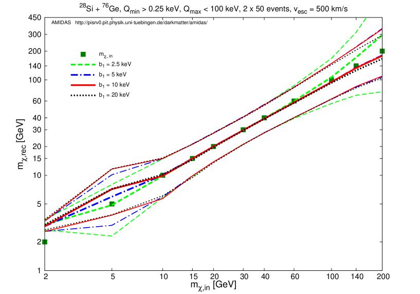
Figure 1: The reconstructed WIMP masses and the lower and upper bounds of the 1$\sigma$ statistical uncertainties as functions of the input WIMP mass with a ${}^{28}{\rm Si}$ + ${}^{76}{\rm Ge}$ target combination for input WIMP masses between 2 and 200 GeV. A small experimental threshold energy of $Q_{\rm min}=0.25$ keV has been simulated. Four different widths of the first energy bin $b_{1}$ have been used: 2.5 keV (dashed green), 5 keV (dash–dotteded blue), 10 keV (solid red), and 20 keV (dotted black). The squared dark–green points indicate the true (input) WIMP masses in our simulations. Each experiment contains 50 events on average (before cuts on $Q_{\rm max}^{\ast}$ determined by Eq. (33)). See the text for further details.

In Fig. 1, we show the reconstructed WIMP masses and the lower and upper bounds of the 1$\sigma$ statistical uncertainties as functions of the input WIMP mass. Four different widths of the first energy bin $b_{1}$ have been used: 2.5 keV (dashed green), 5 keV (dash–dotteded blue), 10 keV (solid red), and 20 keV (dotted black). Note however that, although in our simulations a fixed width of the first energy bin has been set initially, for the three lightest input WIMP masses, $b_{1}$ has been tuned to be the analyzed energy range, i.e., $b_{1}=Q_{\rm max}^{\ast}-Q_{\rm min}$, since this is less than the initial setup of $b_{1}$ in our simulations. For example, for the input WIMP mass of $m_{\chi,{\rm in}}=2$ GeV, $b_{1}$ has been tuned to be 1.33 keV for the Si target and only 0.39 keV for the Ge target (remind that $Q_{\rm min}=0.25$ keV) for all four initially different $b_{1}$. It is thus that the reconstructed WIMP masses as well as the statistical uncertainty bounds are the same for these four cases. Furthermore, for our simulations with the input WIMP mass of $m_{\chi,{\rm in}}=5$ GeV, $b_{1}$ has been tuned to be 7.79 keV for the Si target (for only the cases of $b_{1}=10$ and 20 keV) as well as 3.42 keV (for however the cases of $b_{1}=5$, 10 and 20 keV) for the Ge target. In Table 2, we list the kinematic maximal cut–off energies of the nuclei used in our simulations presented in this paper for different WIMP masses between 2 and 20 GeV for reference.

Isotope	$Z$	$A$	$m_{\chi}=2$ GeV	$m_{\chi}=5$ GeV	$m_{\chi}=10$ GeV	$m_{\chi}=15$ GeV	$m_{\chi}=20$ GeV
${}^{19}{\rm F}$	9	19	2.17	10.23	27.45	44.30	59.22
			(2.81)	(13.22)	(35.48)	(57.25)	(76.54)
${}^{23}{\rm Na}$	11	23	1.86	9.14	25.82	43.23	59.39
			(2.41)	(11.81)	(33.37)	(55.86)	(76.75)
${}^{28}{\rm Si}$	14	28	1.58	8.04	23.85	41.38	58.44
			(2.04)	(10.39)	(30.82)	(53.47)	(75.52)
${}^{40}{\rm Ar}$	18	40	1.15	6.22	19.87	36.55	54.10
			(1.49)	(8.03)	(25.68)	(47.23)	(69.91)
${}^{76}{\rm Ge}$	32	76	0.64	3.67	12.92	25.78	40.91
			(0.82)	(4.75)	(16.70)	(33.32)	(52.87)
${}^{127}{\rm I}$	53	127	0.39	2.32	8.57	17.85	29.48
			(0.50)	(3.00)	(11.07)	(23.07)	(38.09)
${}^{131}{\rm Xe}$	54	131	0.38	2.25	8.34	17.43	28.83
			(0.49)	(2.91)	(10.78)	(22.52)	(37.26)
${}^{136}{\rm Xe}$	54	136	0.36	2.18	8.08	16.92	28.06
			(0.47)	(2.81)	(10.45)	(21.87)	(36.27)

Table 2: The kinematic maximal cut–off energies (in unit of keV) of the nuclei used in our simulations presented in this paper for different WIMP masses between 2 and 20 GeV. Remind that we have set $v_{\rm e}=1.05~{}\!v_{0}=231$ km/s and the values given here (in the parentheses) are corresponding to $v_{\rm esc}=500$ km/s (i.e., $v_{\rm max}=731$ km/s) and $v_{\rm esc}=600$ km/s ($v_{\rm max}=831$ km/s), respectively.

It can be found in Fig. 1 clearly that, for the input WIMP mass of $m_{\chi,{\rm in}}=2$ GeV, the reconstructed mass is a bit overestimated. The main reason should be the following: the corresponding kinematic maximal cut–off energies are very low (see Table 2): $Q_{\rm max,kin,Si}=1.58$ keV and $Q_{\rm max,kin,Ge}=0.64$ keV. Thus, for the germanium target, the threshold energy of $Q_{\rm min}=0.25$ keV cuts almost 40% of the theoretically analyzable energy range. According to the transformation given by Eq. (2), this means a minimal cut–off velocity of $v_{\rm min}^{\ast}=v_{\rm min}(0.25~{}{\rm keV})\simeq 460$ km/s, which not only cuts $\sim$ 63% of the considered velocity range ($0\leq v\leq v_{\rm max}=731$ km/s), but also far beyond the peak of our (input) velocity distribution function at $\simeq$ 310 km/s. Hence, our trianglar approximation for the velocity range of $v\leq v_{\rm min}^{\ast}$ for estimating the normalization constant ${\cal N}$ as well as the moments of the WIMP velocity distribution, $\langle{\textstyle{v^{n}}}\rangle$, in Eqs. (14) and (17) can obviously not hold anymore.

Similarly, due to the pretty small kinematic cut–off energy and the relatively high threshold energy, for the input WIMP mass of $m_{\chi,{\rm in}}=5$ GeV, the reconstructed WIMP mass could also be somehow overestimated. However, it should be caused by the use of the logarithmically linear ansatz (5) for reconstructing $dR/dQ$: in all cases with the tuned (reduced) bin width discussed before, we have used in fact the whole analyzed energy range as the first bin to reconstruct the recoil spectrum, or, equivalently, to estimate the logarithmic slope $k_{1}$. This would be too wide and $k_{1}$ could thus be underestimated (see Fig. 1 of Ref. [60]). Consequently, $K_{1}(Q_{\rm min})$ and $r^{\ast}(Q_{\rm min})$ defined in Eqs. (15) and (18) would in turn be overestimated. Moreover, by increasing the initial bin width, only the used one for the Si target increases, whereas for the Ge target the used bin width has been kept as 3.42 keV, except of the smallest case of $b_{1}=2.5$ keV; it would therefore be the reason that the WIMP mass could still be reconstructed pretty precisely with $b_{1}=2.5$ keV but show a $b_{1}$–dependent overestimate.

On the other hand, for the input WIMP masses $m_{\chi,{\rm in}}\>\raisebox{-3.01385pt}{$\stackrel{{\scriptstyle\textstyle>}}{{\sim}}$}\>10$ GeV, our simulations show that the algorithmic procedure with the modified ${\cal R}_{n,(X,Y)}$ and ${\cal R}_{\sigma,(X,Y)}$ could reconstruct the WIMP masses pretty precisely with statistical uncertainties of $\sim$ 30% to 45%, regardless of the width of the first energy bin; except that, once WIMPs are heavier than $\sim 60$ GeV, the use of a small bin width of $\sim 2.5$ keV would overestimate the reconstructed masses and enlarge the statistical uncertainties. We will discuss about effects of taking different widths of the first energy bin in more detail in Sec. 3.2.1.

3.1.2 Reconstruction of the SI WIMP–nucleon coupling

We continue to present our simulation results of the reconstruction of the (squared) SI (scalar) WIMP–nucleon coupling $|f_{\rm p}|^{2}$ estimated by Eq. (24) for the input WIMP masses between 2 and 200 GeV. Note that, since the WIMP mass could (in principle) be reconstructed pretty well, we show here only the reconstructed $|f_{\rm p}|^{2}$ with the true (input) WIMP masses.

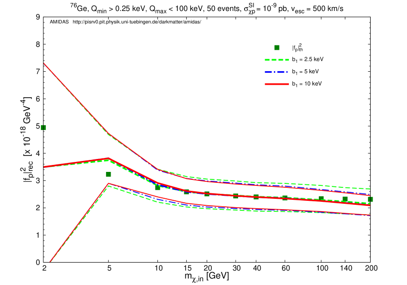
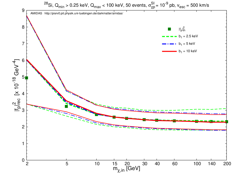
Figure 2: The reconstructed squared SI (scalar) WIMP–nucleon couplings and the lower and upper bounds of the 1$\sigma$ statistical uncertainties as functions of the input WIMP mass with a ${}^{76}{\rm Ge}$ (upper) or a ${}^{28}{\rm Si}$ (lower) target for input WIMP masses between 2 and 200 GeV. The required WIMP mass has been assumed to be the true (input) values. Three different widths of the first energy bin $b_{1}$ (before tuning) have been used: 2.5 keV (dashed green), 5 keV (dash–dotteded blue), and 10 keV (solid red). The squared dark–green points indicate the true (input) WIMP masses and the theoretically estimated $|f_{\rm p}|^{2}$ values. Each experiment contains 50 events on average. The SI WIMP–nucleus cross section has been fixed to be $\sigma_{\chi{\rm p}}^{\rm SI}=10^{-9}$ pb.

In Figs. 2, we show the reconstructed squared SI WIMP–nucleon couplings and the lower and upper bounds of the 1$\sigma$ statistical uncertainties as functions of the input WIMP mass with a ${}^{76}{\rm Ge}$ (upper) and a ${}^{28}{\rm Si}$ (lower) target separately. Three different widths of the first energy bin $b_{1}$ (before tuning) have been used: 2.5 keV (dashed green), 5 keV (dash–dotteded blue), and 10 keV (solid red).

As discussed previously, for the input WIMP mass of $m_{\chi,{\rm in}}=2$ GeV, the corresponding kinematic maximal cut–off energies are $Q_{\rm max,kin,Si}=1.58$ keV and $Q_{\rm max,kin,Ge}=0.64$ keV, respectively. This means that, while for the germanium target the threshold energy of $Q_{\rm min}=0.25$ keV cuts almost 40% of the theoretically analyzable energy range, for the silicon target, only 16% of the energy range has been cut. Consequently, our simulations shown in Figs. 2 demonstrate clearly that, once the priorly known or reconstructed WIMP mass is pretty light, $|f_{\rm p}|^{2}$ could be (strongly) underestimated by using data with heavy target nuclei (Ge or Xe), but (much) better reconstructed with light target nuclei (Si and Ar).

On the other hand, for the input WIMP masses $m_{\chi,{\rm in}}\>\raisebox{-3.01385pt}{$\stackrel{{\scriptstyle\textstyle>}}{{\sim}}$}\>10$ GeV, the SI WIMP–nucleon coupling could be reconstructed very precisely with statistical uncertainties of $\sim$ 20% to 30%, by using not only the Ge and Si targets, but in fact also other available nuclei, e.g. Ar or Xe. However, as already shown in Ref. [63], for input WIMP masses of $m_{\chi,{\rm in}}\>\raisebox{-3.01385pt}{$\stackrel{{\scriptstyle\textstyle>}}{{\sim}}$}\>100$ GeV, $|f_{\rm p}|^{2}$ could be a bit underestimated with heavy (Ge and Xe) nuclei. More comparisons between results reconstructed with light (Si) and heavy (Ge) target nuclei when the threshold energy increases will be given in Sec. 3.2.2.

3.1.3 Reconstruction of the ratio between the SD WIMP–nucleon couplings

Now we consider the ratio between two SD WIMP–nucleon couplings $a_{\rm n}/a_{\rm p}$ with both of the estimators given in Eqs. (37) and (52). Only the combination of the ${}^{19}{\rm F}$ + ${}^{127}{\rm I}$ nuclei has been used in our simulations, since a much wider range of the $a_{\rm n}/a_{\rm p}$ ratio (between $\pm 4$) can (in principle) be well reconstructed [64]. Remind that, as discussed in Ref. [64] and Sec. 2.3, for the F + I target combination, one should take the “$-$ (minus)” solution for both of Eqs. (37) and Eqs. (52). Note also that, in all simulations presented in this paper, a non–zero SI WIMP–nucleon cross section $\sigma_{\chi{\rm p}}^{\rm SI}=10^{-9}$ pb has always been taken into account.

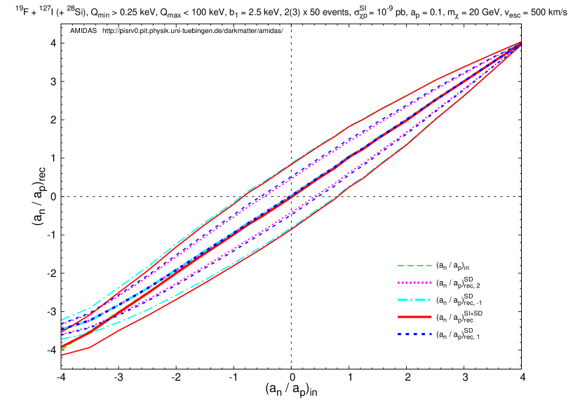
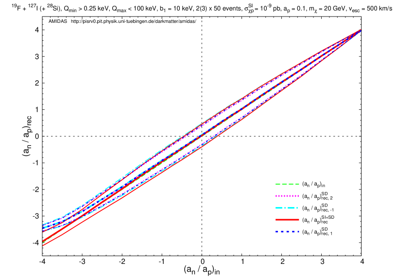
Figure 3: The reconstructed $a_{\rm n}/a_{\rm p}$ ratios estimated by Eq. (37) and their lower and upper bounds of the 1$\sigma$ statistical uncertainties with $n=-1$ (dash–dotted cyan), 1 (long–dotted blue), and 2 (dotted magenta) as well as those estimated by Eq. (52) (solid red) as functions of the input $a_{\rm n}/a_{\rm p}$ ratio with the ${}^{19}{\rm F}$ + ${}^{127}{\rm I}$ target combination and ${}^{28}{\rm Si}$ as the third spinless target for input $a_{\rm n}/a_{\rm p}$ ratios between $\pm 4$. The mass of incident WIMPs has been set as 20 GeV. Remind that a non–zero SI WIMP–nucleon cross section $\sigma_{\chi{\rm p}}^{\rm SI}=10^{-9}$ pb has been included. A relatively small bin width of $b_{1}=2.5$ keV (upper) and a wider width of $b_{1}=10$ keV (lower) (before tuning) have been used. Each experiment contains 50 events on average.

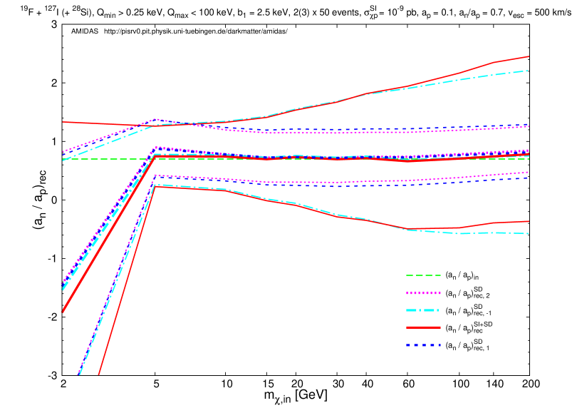
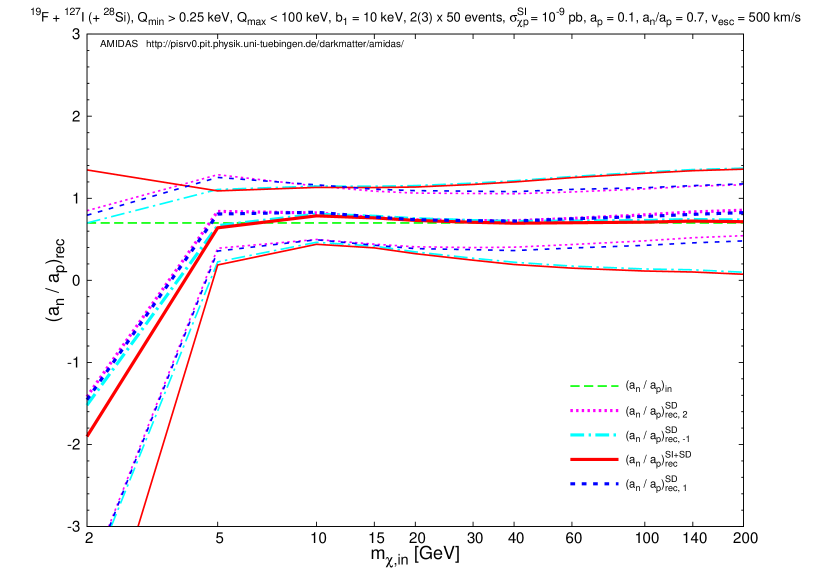
Figure 4: The reconstructed $a_{\rm n}/a_{\rm p}$ ratios and their lower and upper bounds of the 1$\sigma$ statistical uncertainties as functions of the input WIMP mass with the ${}^{19}{\rm F}$ + ${}^{127}{\rm I}$ target combination and ${}^{28}{\rm Si}$ as the third spinless target for input WIMP masses between 2 and 200 GeV. The input $a_{\rm n}/a_{\rm p}$ ratio has been fixed as 0.7. Other parameters and all notations are the same as in Figs. 3.

In Figs. 3, we show at first the reconstructed $a_{\rm n}/a_{\rm p}$ ratios estimated by Eq. (37) and their lower and upper bounds of the 1$\sigma$ statistical uncertainties with $n=-1$ (dash–dotted cyan), 1 (long–dotted blue), and 2 (dotted magenta) as well as those estimated by Eq. (52) (solid red) as functions of the input $a_{\rm n}/a_{\rm p}$ ratio with a ${}^{19}{\rm F}$ + ${}^{127}{\rm I}$ target combination and ${}^{28}{\rm Si}$ as the third spinless target for input $a_{\rm n}/a_{\rm p}$ ratios between $\pm 4$. The mass of incident WIMPs has been set as 20 GeV. A relatively small bin width of $b_{1}=2.5$ keV (upper) and a wider width of $b_{1}=10$ keV (lower) (before tuning) have been used.

It can be found in the upper frame of Figs. 3 that, although the reconstructed $a_{\rm n}/a_{\rm p}$ ratios given by Eq. (37) with three different $n$ are slightly overestimated at the end closed to $\langle{\textstyle{S_{\rm p}}}\rangle_{\rm I}/\langle{\textstyle{S_{\rm n}}}\rangle_{\rm I}=-4.12$ (due to including the non–zero SI WIMP–nucleus cross section [64]), not surprisingly, the ratio given by Eq. (52) could precisely match all the true (input) values. However, the 1$\sigma$ statistical uncertainties estimated with $n=-1$ and from the general Eq. (52) are almost twice as large as those with $n=1$ and 2. Nevertheless, by increasing the width of the first energy bin, the (difference between the) 1$\sigma$ statistical uncertainties by using both estimators could be reduced (significantly).

On the other hand, in Figs. 4, we show the reconstructed $a_{\rm n}/a_{\rm p}$ ratios and their 1$\sigma$ statistical uncertainties as functions of the input WIMP mass with the F + I (+ Si) target combination for input WIMP masses between 2 and 200 GeV. The input $a_{\rm n}/a_{\rm p}$ ratio has been fixed as 0.7.

First, as discussed before, for the lightest input WIMP mass of $m_{\chi,{\rm in}}=2$ GeV, the kinematic maximal cut–off energy of the iodine target is only 0.39 keV and the threshold energy of $Q_{\rm min}=0.25$ keV cuts thus more than 60% of the theoretically analyzable energy range. Consequently, the reconstructed $a_{\rm n}/a_{\rm p}$ ratios are strongly underestimated. Nevertheless, for all larger input WIMP masses $m_{\chi,{\rm in}}\>\raisebox{-3.01385pt}{$\stackrel{{\scriptstyle\textstyle>}}{{\sim}}$}\>5$ GeV, the reconstructions of the $a_{\rm n}/a_{\rm p}$ ratio become to match the true (input) values very well. Furthermore, two plots in Figs. 4 show more clearly that, with the use of a small bin width of $b_{1}=2.5$ keV, the 1$\sigma$ statistical uncertainties with $n=1$ and 2 are approximately equal and (much smaller) than the uncertainties estimated with $n=-1$ and from the general Eq. (52), especially for the large input WIMP masses. And similarly, by increasing the width of the first energy bin, the (difference between the) uncertainties (with different $n$) could be reduced (significantly); the larger the true (input) WIMP mass, the more significantly the uncertainty could be reduced and, (with a bin width as large as $b_{1}\simeq 10$ keV), the uncertainties would (almost) be independent of the true (input) WIMP mass.

3.1.4 Reconstructions of the ratios between the SD and SI WIMP–nucleon cross sections

We present further the simulation results of the reconstructions of the ratios of the SD and SI WIMP cross sections on protons and on neutrons, $\sigma_{\chi({\rm p,n})}^{\rm SD}/\sigma_{\chi{\rm p}}^{\rm SI}$. Note that, first, for using Eqs. (44) and (42), the needed $a_{\rm n}/a_{\rm p}$ ratio has been reconstructed only by Eq. (52). Second, in all plots the width of the first energy bin (before tuning) has been fixed as $b_{1}=10$ keV.

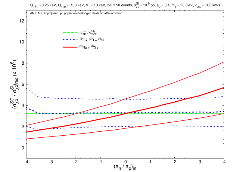
Figure 5: The reconstructed $\sigma_{\chi{\rm p}}^{\rm SD}/\sigma_{\chi{\rm p}}^{\rm SI}$ ratios estimated by Eq. (44) and their lower and upper bounds of the 1$\sigma$ statistical uncertainties with the ${}^{19}{\rm F}$ + ${}^{127}{\rm I}$ + ${}^{28}{\rm Si}$ target combination (long–dotted blue) as well as by Eq. (55) with the ${}^{23}{\rm Na}$ + ${}^{76}{\rm Ge}$ target combination (solid red). Upper: with a fixed input WIMP mass of $m_{\chi,{\rm in}}=20$ GeV as functions of the input $a_{\rm n}/a_{\rm p}$ ratio between $\pm 4$; lower: with a fixed input ratio of $a_{\rm n}/a_{\rm p}=0.7$ as functions of the input WIMP mass between 2 and 200 GeV. Only the $a_{\rm n}/a_{\rm p}$ ratio reconstructed by Eq. (52) has been included and the width of the first energy bin (before tuning) has been fixed as $b_{1}=10$ keV. Other parameters are the same as in Figs. 3 and 4.

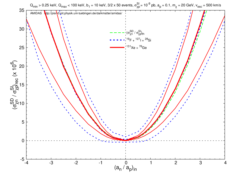
Figure 6: The reconstructed $\sigma_{\chi{\rm n}}^{\rm SD}/\sigma_{\chi{\rm p}}^{\rm SI}$ ratios estimated by Eq. (42) and their lower and upper bounds of the 1$\sigma$ statistical uncertainties with the ${}^{19}{\rm F}$ + ${}^{127}{\rm I}$ + ${}^{28}{\rm Si}$ target combination (long–dotted blue) as well as by Eq. (57) with the ${}^{131}{\rm Xe}$ + ${}^{76}{\rm Ge}$ target combination (solid red). Upper: with a fixed input WIMP mass of $m_{\chi,{\rm in}}=20$ GeV as functions of the input $a_{\rm n}/a_{\rm p}$ ratio between $\pm 4$; lower: with a fixed input ratio of $a_{\rm n}/a_{\rm p}=0.7$ as functions of the input WIMP mass between 2 and 200 GeV. Only the $a_{\rm n}/a_{\rm p}$ ratio reconstructed by Eq. (52) has been included and the width of the first energy bin (before tuning) has been fixed as $b_{1}=10$ keV. Other parameters are the same as in Figs. 3 and 4.

In Figs. 5, we show the reconstructed $\sigma_{\chi{\rm p}}^{\rm SD}/\sigma_{\chi{\rm p}}^{\rm SI}$ ratios estimated by Eq. (44) and their lower and upper bounds of the 1$\sigma$ statistical uncertainties with the ${}^{19}{\rm F}$ + ${}^{127}{\rm I}$ + ${}^{28}{\rm Si}$ target combination (long–dotted blue) as well as by Eq. (55) with a ${}^{23}{\rm Na}$ + ${}^{76}{\rm Ge}$ target combination (solid red). While in the upper frame, the $\sigma_{\chi{\rm p}}^{\rm SD}/\sigma_{\chi{\rm p}}^{\rm SI}$ ratios and their statistical uncertainties are reconstructed with a fixed input WIMP mass of $m_{\chi,{\rm in}}=20$ GeV and given as functions of the input $a_{\rm n}/a_{\rm p}$ ratio between $\pm 4$, in the lower frame, the input ratio of $a_{\rm n}/a_{\rm p}$ is fixed as 0.7 and the results are given as functions of the input WIMP mass between 2 and 200 GeV.

It can be seen clearly that, in the wide range of interests of $|a_{\rm n}/a_{\rm p}|\leq 4$, the $\sigma_{\chi{\rm p}}^{\rm SD}/\sigma_{\chi{\rm p}}^{\rm SI}$ ratios could be reconstructed by Eqs. (44) with the ${}^{19}{\rm F}$ + ${}^{127}{\rm I}$ + ${}^{28}{\rm Si}$ target combination (much) better: except of the a–bit–overestimated one at the end of $(a_{\rm n}/a_{\rm p})_{\rm in}=-4$, not only the $\sigma_{\chi{\rm p}}^{\rm SD}/\sigma_{\chi{\rm p}}^{\rm SI}$ ratios can be estimated very precisely, but also their statistical uncertainties are independent of the input $a_{\rm n}/a_{\rm p}$ ratios. On the other hand, except of the lightest input WIMP mass of $m_{\chi,{\rm in}}=2$ GeV, with a fixed $a_{\rm n}/a_{\rm p}$ ratio (lower frame), for the input WIMP masses of $m_{\chi,{\rm in}}\>\raisebox{-3.01385pt}{$\stackrel{{\scriptstyle\textstyle>}}{{\sim}}$}\>5$ GeV, the $\sigma_{\chi{\rm p}}^{\rm SD}/\sigma_{\chi{\rm p}}^{\rm SI}$ ratios could be reconstructed by both combinations very well. Note however that, although the reconstructed results with the ${}^{23}{\rm Na}$ + ${}^{76}{\rm Ge}$ target combination shown in the lower frame look also pretty nice, as discussed above, this is only because that the input $a_{\rm n}/a_{\rm p}$ ratio is fixed as 0.7. As shown in the upper frame, once the true $a_{\rm n}/a_{\rm p}$ ratio exceeds the range of $|a_{\rm n}/a_{\rm p}|\>\raisebox{-3.01385pt}{$\stackrel{{\scriptstyle\textstyle<}}{{\sim}}$}\>1$, the reconstructions by the ${}^{23}{\rm Na}$ + ${}^{76}{\rm Ge}$ target combination would be (strongly) over– or underestimated!

On the other hand, in Figs. 6, we show the reconstructed $\sigma_{\chi{\rm n}}^{\rm SD}/\sigma_{\chi{\rm p}}^{\rm SI}$ ratios estimated by Eq. (42) and their lower and upper bounds of the 1$\sigma$ statistical uncertainties with the ${}^{19}{\rm F}$ + ${}^{127}{\rm I}$ + ${}^{28}{\rm Si}$ target combination (long–dotted blue) as well as by Eq. (57) with a ${}^{131}{\rm Xe}$ + ${}^{76}{\rm Ge}$ target combination (solid red).

Our results show that, although both combinations could offer well reconstructed $\sigma_{\chi{\rm n}}^{\rm SD}/\sigma_{\chi{\rm p}}^{\rm SI}$ ratios, with either a fixed WIMP mass or a fixed $a_{\rm n}/a_{\rm p}$ ratio, but, in contrast to the results shown in Figs. 5, the statistical uncertainties estimated with the ${}^{131}{\rm Xe}$ + ${}^{76}{\rm Ge}$ targets could now be much smaller (the half of) than those with ${}^{19}{\rm F}$ + ${}^{127}{\rm I}$ + ${}^{28}{\rm Si}$ combination. Moreover, for the lightest input WIMP mass of $m_{\chi,{\rm in}}=2$ GeV, while the reconstructed ratio with the ${}^{19}{\rm F}$ + ${}^{127}{\rm I}$ + ${}^{28}{\rm Si}$ combination could now be overestimated, the one with the ${}^{131}{\rm Xe}$ + ${}^{76}{\rm Ge}$ targets could be underestimated. Nevertheless, as usual, for the input WIMP masses of $m_{\chi,{\rm in}}\>\raisebox{-3.01385pt}{$\stackrel{{\scriptstyle\textstyle>}}{{\sim}}$}\>5$ GeV, the $\sigma_{\chi{\rm n}}^{\rm SD}/\sigma_{\chi{\rm p}}^{\rm SI}$ ratio could be reconstructed very well with uncertainty depending only slightly on the true (input) WIMP mass by using both target combinations.

3.2 Raising the threshold energy

In this section, we raise the threshold energy to $Q_{\rm min}=2.5$ and even $Q_{\rm min}=5$ keV and then repeat our simulations in order to confirm our observations discussed previously.

3.2.1 Reconstruction of the WIMP mass

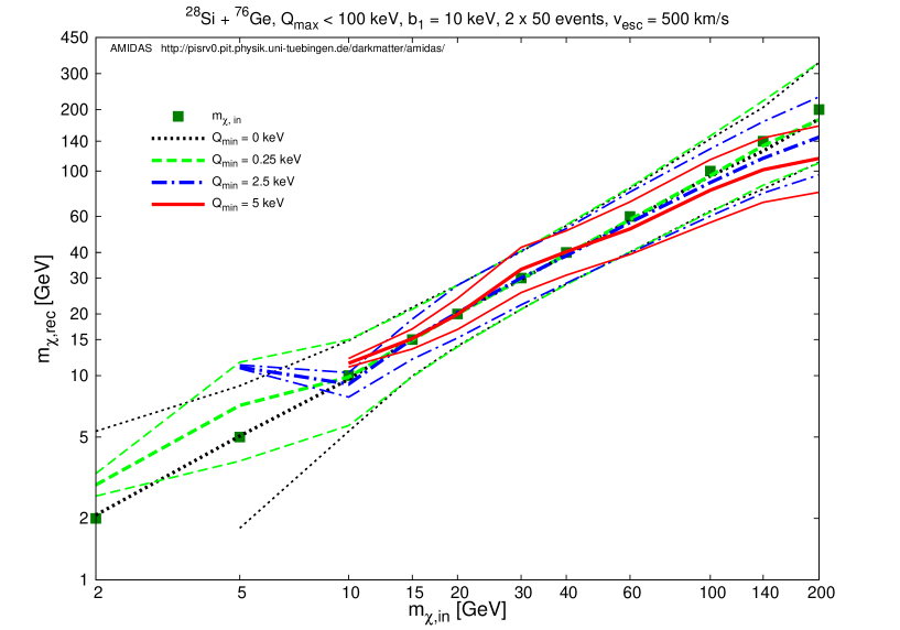
Figure 7: As in Fig. 1, except that three different minimal cut–off energies have been considered: $Q_{\rm min}=0.25$ keV (dashed green), 2.5 keV (dash–dotteded blue), and 5 keV (solid red). As a reference, the reconstructed masses and the statistical uncertainties with zero minimal cut–off energy $Q_{\rm min}=0$ (dotted black) have also been given here. The width of the first energy bin (before tuning) has been fixed as $b_{1}=10$ keV.

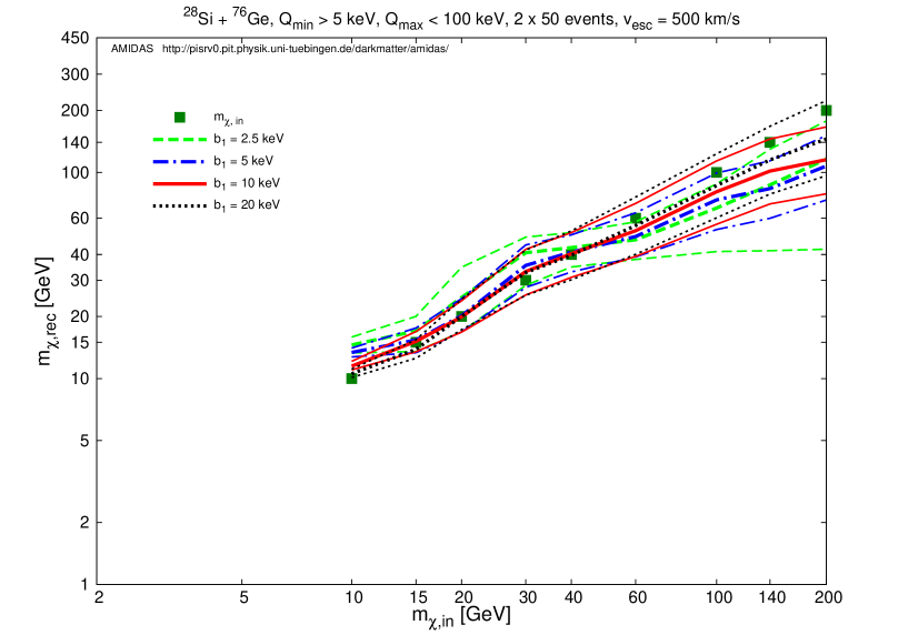
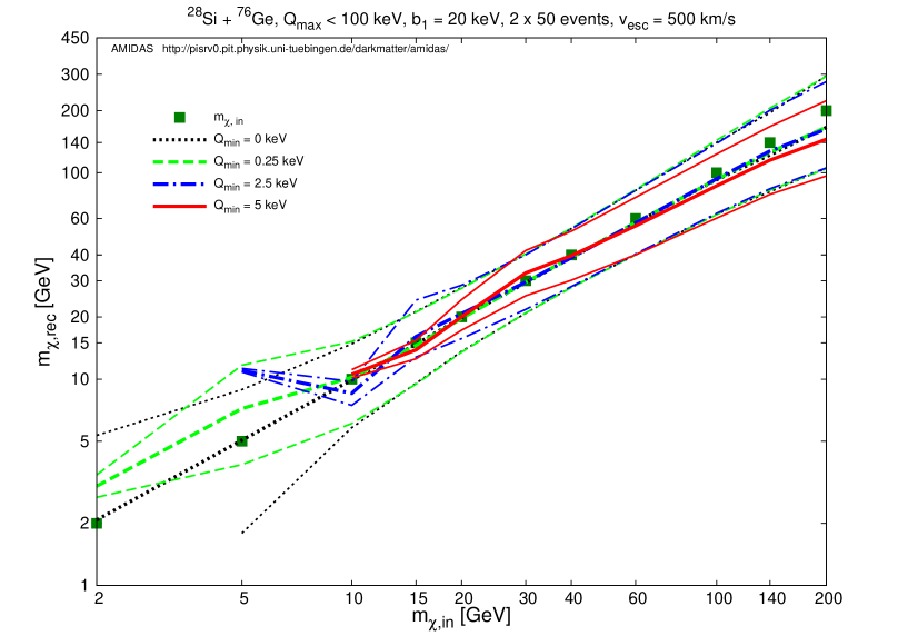
Figure 8: Upper: as in Fig. 1, except that the minimal cut–off energy has been raised to $Q_{\rm min}=5$ keV. Lower: as in Fig. 7, except that the width of the first energy bin (before tuning) has been enlarged to $b_{1}=20$ keV.

In Fig. 7, we show the reconstructed WIMP masses and the 1$\sigma$ statistical uncertainty bounds with three different minimal cut–off energies together: $Q_{\rm min}=0.25$ keV (dashed green), 2.5 keV (dash–dotteded blue), and 5 keV (solid red). As a reference, the reconstructed masses and the statistical uncertainties with zero minimal cut–off energy $Q_{\rm min}=0$ (dotted black) have also been given. The width of the first energy bin (before tuning) has been fixed as $b_{1}=10$ keV.

It can be found here that, as discussed in Sec. 3.1.1, for the input WIMP mass of $m_{\chi,{\rm in}}=2$ or 5 GeV, the corresponding kinematic maximal cut–off energies for the Si and Ge targets are only $Q_{\rm max,kin,Si}=1.58$ or 8.04 keV and $Q_{\rm max,kin,Ge}=0.64$ or 3.67 keV. It is thus obviously that no WIMP events can be observed above an experimental threshold energy of $Q_{\rm min}=2.5$ (or 5) keV with a Si or Ge target. Additionally, for the larger input WIMP masses of $m_{\chi,{\rm in}}=5$ (and 10) GeV, the corresponding kinematic maximal cut–off energies for the Ge target are only $Q_{\rm max,kin,Ge}=3.67$ (and 12.92) keV. Hence, the $Q_{\rm min}=2.5$ (and 5) keV threshold energies cut 68% (and 39%) of the theoretically analyzable energy ranges. This results in overestimates of the reconstructed WIMP mass for input WIMP masses $m_{\chi,{\rm in}}\>\raisebox{-3.01385pt}{$\stackrel{{\scriptstyle\textstyle<}}{{\sim}}$}\>10$ GeV.

On the other hand, for the input WIMP masses of $m_{\chi,{\rm in}}\>\raisebox{-3.01385pt}{$\stackrel{{\scriptstyle\textstyle>}}{{\sim}}$}\>50$ GeV, our simulations show that the higher the minimal cut–off energy, the more underestimate the reconstructed WIMP mass. In order to alleviate this underestimate, we consider then a much wider width of $b_{1}=20$ keV for the first energy bin in Figs. 8. The upper frame of Figs. 8 shows the reconstructed WIMP masses by using data sets with a common minimal cut–off energy of $Q_{\rm min}=5$ keV but four different widths of the first energy bin: 2.5 keV (dashed green), 5 keV (dash–dotteded blue), 10 keV (solid red), and 20 keV (dotted black). It can be found obviously that, with a fixed threshold energy as high as $Q_{\rm min}=5$ keV, the larger the width of the first energy bin, the higher (preciser) the reconstructed WIMP masses; the underestimate of the reconstructed WIMP masses between 60 and 200 GeV could indeed be alleviated. Meanwhile, we show in the lower frame of Figs. 8 the reconstructed WIMP masses with a larger fixed width of the first energy bin of $b_{1}=20$ keV for four different minimal cut–off energies: $Q_{\rm min}=0$ (dotted black), 0.25 keV (dashed green), 2.5 keV (dash–dotteded blue), and 5 keV (solid red). Comparing with the results shown in Fig. 7, one can see clearly the improvement of the WIMP mass reconstruction. Additionally and more importantly, our simulations indicates that, the larger the minimal cut–off energy, the larger the alleviation by using a larger $b_{1}$ could be.

It would be reasonable to expect that the reconstruction of the WIMP mass (as well as the other properties) could be somehow (or even strongly) improved, once the true escape velocity of our Galaxy would be larger (than the value used in our presented simulations). However, according to our further simulations with a larger escape velocity of $v_{\rm esc}=600$ km/s, this expectation would unfortunately not be certainly true. Firstly, with a larger escape velocity and thus a larger kinematic cut–off on the velocity distribution as well as on the recoil spectra, the “truncation” problem discussed in Sec. 3.1 and, especially, above could indeed be alleviated a little bit and then the systematic deviations of the reconstructed results from the true (input) values could be reduced a little bit, but only a very little bit, much smaller than what one would expect. Actually, due to the exponential–like shape of the predicted recoil spectrum, in a data set with a few tens of total events at most only one extra event could “occasionally” be recorded in the extended high–energy range (between, e.g., 3.67 and 4.75 keV for the Ge target and the WIMP mass of 5 GeV, see Table 2). On the other hand, as shown in Table 2, for e.g. the I and Xe nuclei, the cut–offs of the kinematic energy could become (from lower to) higher than the experimental threshold energies and some WIMP events could thus be observed. However, as discussed earlier, since large parts of the theoretically analyzable energy ranges would still be cut by the relatively pretty high threshold energies, the reconstructed results would be (strongly) deviated from the true (input) values and not (very) reliable.

3.2.2 Reconstruction of the SI WIMP–nucleon coupling

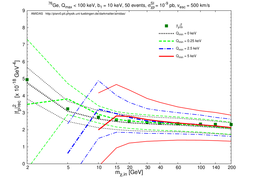
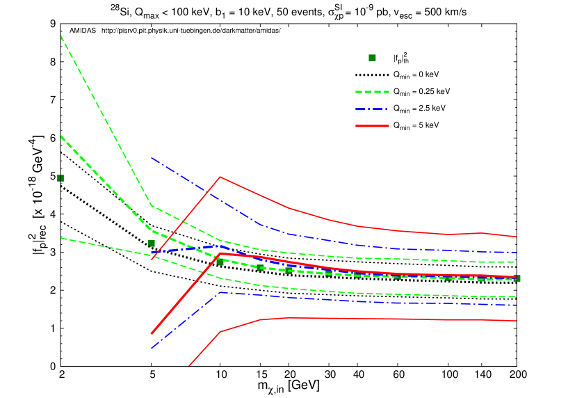
Figure 9: As in Figs. 2, except that three different minimal cut–off energies have been considered: $Q_{\rm min}=0.25$ keV (dashed green), 2.5 keV (dash–dotteded blue), and 5 keV (solid red). As a reference, the reconstructed couplings and the statistical uncertainties with zero minimal cut–off energy $Q_{\rm min}=0$ (dotted black) have also been given here. Note that the width of the first energy bin (before tuning) has been fixed as $b_{1}=10$ keV.

In Fig. 9, we show the reconstructed (squared) SI WIMP–nucleon couplings and the 1$\sigma$ statistical uncertainty bounds with three different minimal cut–off energies together: $Q_{\rm min}=0.25$ keV (dashed green), 2.5 keV (dash–dotteded blue), and 5 keV (solid red). As a reference, the reconstructed couplings and the statistical uncertainties with zero minimal cut–off energy $Q_{\rm min}=0$ have also been given. Note that the width of the first energy bin (before tuning) has been fixed as $b_{1}=10$ keV.

As discussed in Secs. 3.1.2 and 3.2.1, for the input WIMP masses of $m_{\chi,{\rm in}}=2$ (and 5) GeV, no WIMP events can be observed above $Q_{\rm min}=5$ (or 2.5) keV experimental cut–off energy by using a germanium (or silicon) target. Also, for the larger input WIMP masses of $m_{\chi,{\rm in}}=5$ (and 10) GeV, large parts of the theoretically analyzable energy ranges would be cut by a threshold energy of $Q_{\rm min}=2.5$ (or 5) keV and this results in the underestimates of the reconstructed SI coupling for input WIMP masses $m_{\chi,{\rm in}}\>\raisebox{-3.01385pt}{$\stackrel{{\scriptstyle\textstyle<}}{{\sim}}$}\>10$ GeV (for Ge, upper) or 5 GeV (for Si, lower). Nevertheless, for the input WIMP masses of $m_{\chi,{\rm in}}\>\raisebox{-3.01385pt}{$\stackrel{{\scriptstyle\textstyle>}}{{\sim}}$}\>10$ (15) GeV, the SI WIMP–proton couplings could always be reconstructed pretty precisely by using both of the Si (light) and Ge (heavy) targets. By increasing the minimal cut–off energy, one would only obtain larger statistical uncertainties on the reconstructed couplings. Moreover, as observed before, for the input WIMP masses of $m_{\chi,{\rm in}}\>\raisebox{-3.01385pt}{$\stackrel{{\scriptstyle\textstyle>}}{{\sim}}$}\>100$ GeV, the $|f_{\rm p}|^{2}$ couplings could be reconstructed more precisely with light (Si and Ar) targets then with heavy (Ge and Xe) targets, with however slightly larger statistical uncertainties.

3.2.3 Reconstruction of the ratio between the SD WIMP–nucleon couplings

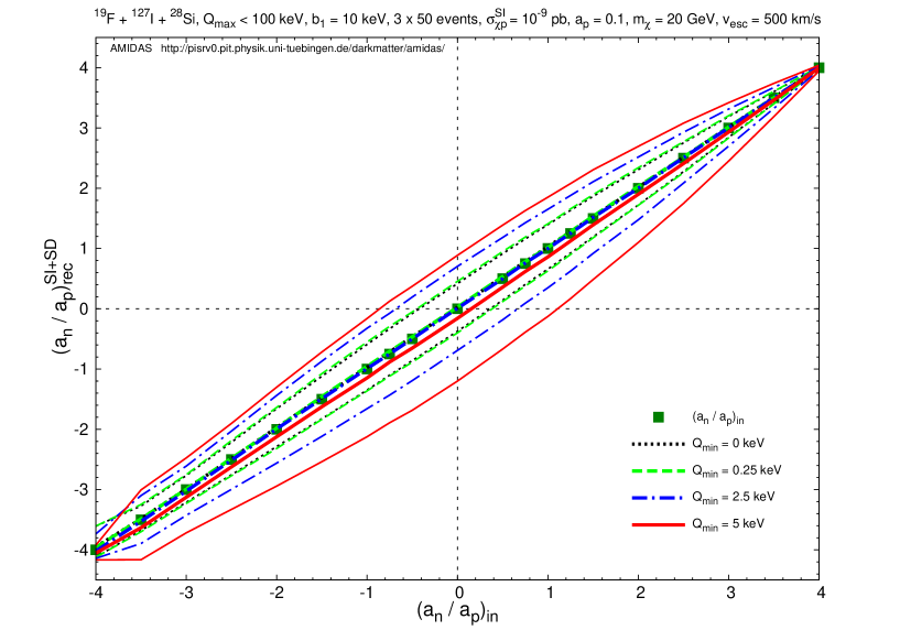
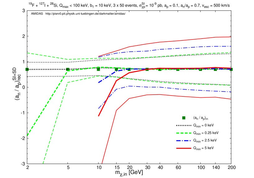
Figure 10: The reconstructed $a_{\rm n}/a_{\rm p}$ ratios estimated only by Eq. (52) and the 1$\sigma$ statistical uncertainty bounds with the ${}^{19}{\rm F}$ + ${}^{127}{\rm I}$ + ${}^{28}{\rm Si}$ target combination. Upper: the reconstructed $a_{\rm n}/a_{\rm p}$ ratios with a fixed input WIMP mass of $m_{\chi,{\rm in}}=20$ GeV as functions of the input $a_{\rm n}/a_{\rm p}$ ratio between $\pm 4$; lower: with a fixed input ratio of $a_{\rm n}/a_{\rm p}=0.7$ as functions of the input WIMP mass between 2 and 200 GeV. The squared dark–green points indicate the true (input) (WIMP masses and) $a_{\rm n}/a_{\rm p}$ values. Four different minimal cut–off energies have been considered: $Q_{\rm min}=0$ (dotted black), 0.25 keV (dashed green), 2.5 keV (dash–dotteded blue), and 5 keV (solid red). The width of the first energy bin (before tuning) has been fixed as $b_{1}=10$ keV. Other parameters are the same as in Figs. 3 and 4.

In Figs. 10, we show the reconstructed $a_{\rm n}/a_{\rm p}$ ratios estimated only by Eq. (52) and the 1$\sigma$ statistical uncertainty bounds with the ${}^{19}{\rm F}$ + ${}^{127}{\rm I}$ + ${}^{28}{\rm Si}$ target combination. Three different minimal cut–off energies: $Q_{\rm min}=0.25$ keV (dashed green), 2.5 keV (dash–dotteded blue), and 5 keV (solid red) have been presented with the results of zero minimal cut–off energy $Q_{\rm min}=0$ (dotted black) as a reference. The width of the first energy bin (before tuning) has been fixed as $b_{1}=10$ keV.

In the lower frame of Figs. 10, the reconstructed $a_{\rm n}/a_{\rm p}$ ratios and the uncertainty bounds with a fixed input ratio of $a_{\rm n}/a_{\rm p}=0.7$ has been given as functions of the input WIMP mass between 2 and 200 GeV. As discussed before, this plot shows again that, for the input WIMP masses of $m_{\chi,{\rm in}}=2$ and 5 GeV, the corresponding kinematic maximal cut–off energies for the I target are only $Q_{\rm max,kin,I}=0.39$ and 2.32 keV, and thus no WIMP events can be observed above $Q_{\rm min}=2.5$ and 5 keV experimental cut–off energies. Furthermore, for the larger input WIMP mass of $m_{\chi,{\rm in}}=10$ or 15 GeV, the corresponding kinematic maximal cut–off for iodine is only $Q_{\rm max,kin,I}=8.57$ or 17.85 keV. Hence, the $Q_{\rm min}=2.5$ and 5 keV threshold energies cuts 29% and 58% (for the input WIMP mass of $m_{\chi,{\rm in}}=10$ GeV) of the theoretically analyzable energy range. This results again in the underestimates of the reconstructed $a_{\rm n}/a_{\rm p}$ ratios for $m_{\chi,{\rm in}}\>\raisebox{-3.01385pt}{$\stackrel{{\scriptstyle\textstyle<}}{{\sim}}$}\>10$ (and 15) GeV.

Nevertheless, and importantly, comparing with the results presented in Ref. [64] (with the unmodified estimators), the reconstructions of the $a_{\rm n}/a_{\rm p}$ ratios have been strongly improved here, once some (real) WIMP events can be observed above the experimental threshold energies. Moreover, if the WIMP mass is larger than ${\cal O}(20)$ GeV, even with a threshold energy of $\sim$ 5 keV, we could in principle reconstruct the $a_{\rm n}/a_{\rm p}$ ratio very precisely. Additionally, as also shown in the upper frame of Figs. 10, the plot of the reconstructed $a_{\rm n}/a_{\rm p}$ ratios and statistical uncertainty bounds with a fixed input WIMP mass of $m_{\chi,{\rm in}}=20$ GeV between $a_{\rm n}/a_{\rm p}=\pm 4$, increasing the minimal cut–off energy would only enlarge the statistical uncertainties on the reconstructed $a_{\rm n}/a_{\rm p}$ ratios, which would almost be independent of the true (input) WIMP mass.

3.2.4 Reconstructions of the ratios between the SD and SI WIMP–nucleon cross sections

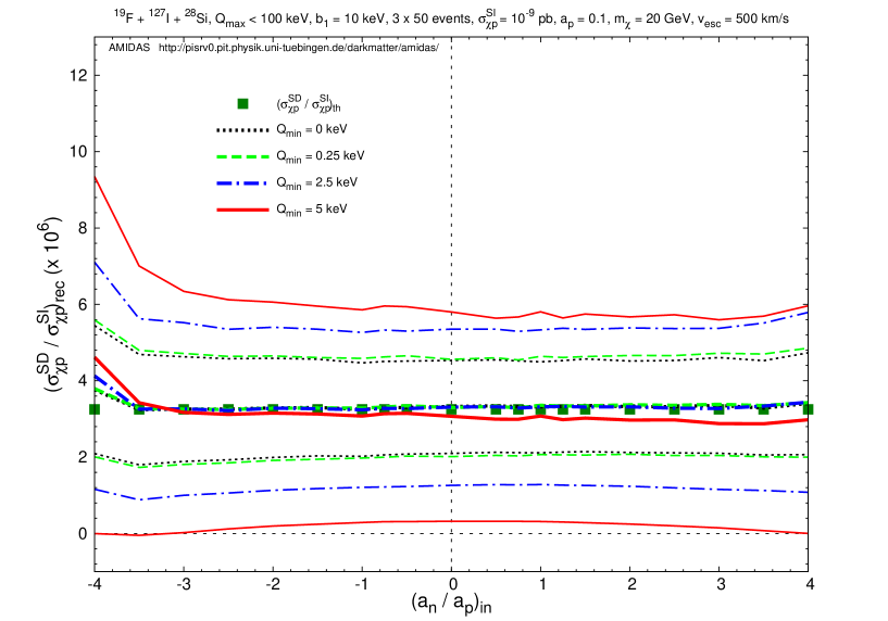
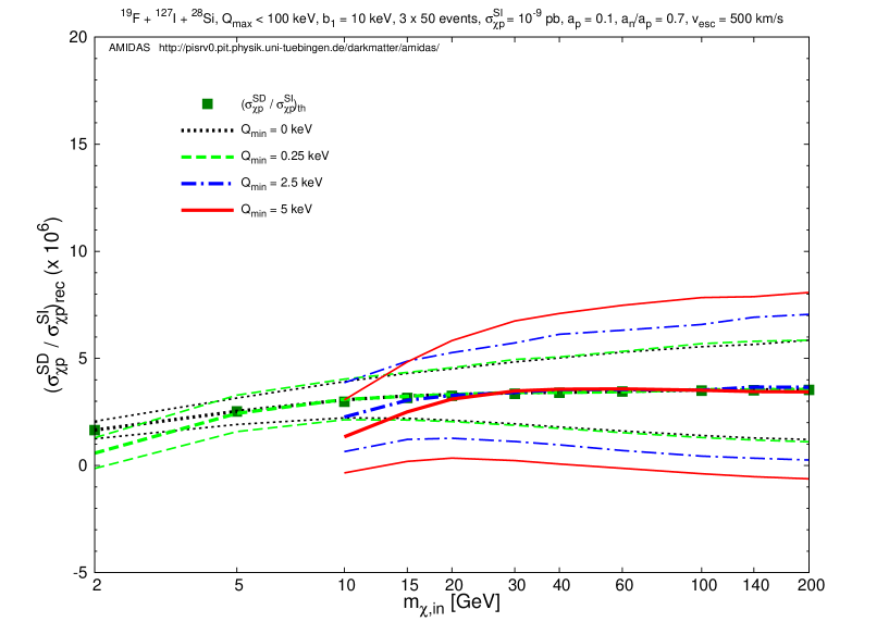
Figure 11: The reconstructed $\sigma_{\chi{\rm p}}^{\rm SD}/\sigma_{\chi{\rm p}}^{\rm SI}$ ratios estimated only by Eq. (44) and the 1$\sigma$ statistical uncertainty bounds with the ${}^{19}{\rm F}$ + ${}^{127}{\rm I}$ + ${}^{28}{\rm Si}$ target combination for input $a_{\rm n}/a_{\rm p}$ ratios between $\pm 4$ (upper) and input WIMP masses between 2 and 200 GeV (lower). Other parameters and notations are the same as in Figs. 10.

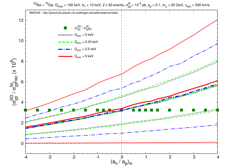
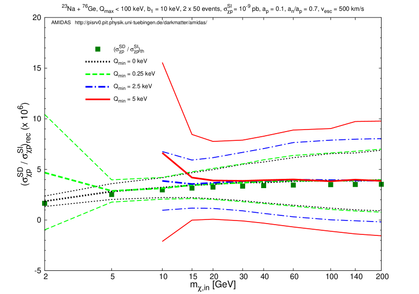
Figure 12: As in Figs. 11, except that $\sigma_{\chi{\rm p}}^{\rm SD}/\sigma_{\chi{\rm p}}^{\rm SI}$ and $\sigma\left(\sigma_{\chi{\rm p}}^{\rm SD}/\sigma_{\chi{\rm p}}^{\rm SI}\right)$ have been estimated by Eq. (55) with the ${}^{23}{\rm Na}$ + ${}^{76}{\rm Ge}$ target combination.

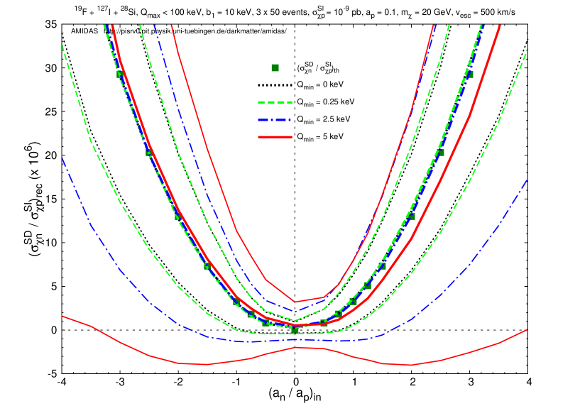
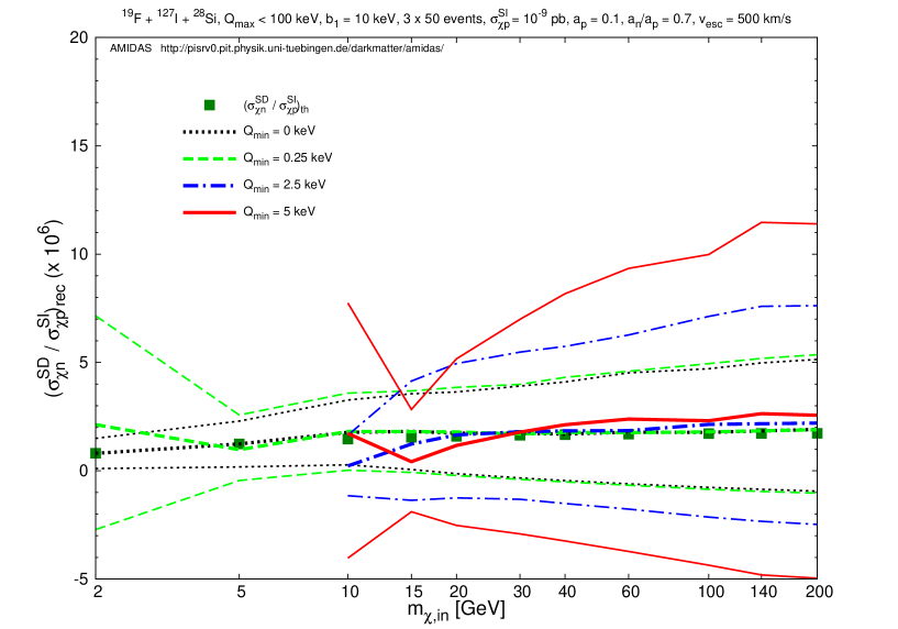
Figure 13: The reconstructed $\sigma_{\chi{\rm n}}^{\rm SD}/\sigma_{\chi{\rm p}}^{\rm SI}$ ratios estimated only by Eq. (42) and the 1$\sigma$ statistical uncertainty bounds with the ${}^{19}{\rm F}$ + ${}^{127}{\rm I}$ + ${}^{28}{\rm Si}$ target combination for input $a_{\rm n}/a_{\rm p}$ ratios between $\pm 4$ (upper) and input WIMP masses between 2 and 200 GeV (lower). Other parameters and all notations are the same as in Figs. 10.

Figure 14: As in Figs. 13, except that $\sigma_{\chi{\rm n}}^{\rm SD}/\sigma_{\chi{\rm p}}^{\rm SI}$ and $\sigma\left(\sigma_{\chi{\rm n}}^{\rm SD}/\sigma_{\chi{\rm p}}^{\rm SI}\right)$ have been estimated by Eq. (57) with the ${}^{131}{\rm Xe}$ + ${}^{76}{\rm Ge}$ target combination.

Finally, in Figs. 11 and 12, we show the reconstructed $\sigma_{\chi{\rm p}}^{\rm SD}/\sigma_{\chi{\rm p}}^{\rm SI}$ ratios estimated by Eq. (44) and the 1$\sigma$ statistical uncertainties with the ${}^{19}{\rm F}$ + ${}^{127}{\rm I}$ + ${}^{28}{\rm Si}$ and by Eq. (55) with the ${}^{23}{\rm Na}$ + ${}^{76}{\rm Ge}$ target combinations separately. As in Figs. 10, in the upper frames of Figs. 11 and 12, the input WIMP mass has been fixed as 20 GeV and we have simulated input $a_{\rm n}/a_{\rm p}$ ratios between $\pm 4$; in the lower frames of two figures, we have fixed the input $a_{\rm n}/a_{\rm p}$ ratio as 0.7 and simulated input WIMP masses between 2 and 200 GeV. As before, four different minimal cut–off energies have been considered: $Q_{\rm min}=0$ (dotted black), 0.25 keV (dashed green), 2.5 keV (dash–dotteded blue), and 5 keV (solid red), and the width of the first energy bin (before tuning) has been fixed as $b_{1}=10$ keV. Meanwhile, in Figs. 13 and 14, we show also the reconstructed $\sigma_{\chi{\rm n}}^{\rm SD}/\sigma_{\chi{\rm p}}^{\rm SI}$ ratios estimated by Eq. (42) and the 1$\sigma$ statistical uncertainty bounds with the ${}^{19}{\rm F}$ + ${}^{127}{\rm I}$ + ${}^{28}{\rm Si}$ and by Eq. (57) with the ${}^{131}{\rm Xe}$ + ${}^{76}{\rm Ge}$ target combinations separately.

These plots demonstrate clearly that, first, as for reconstructing the other WIMP properties, the (pretty) small maximal kinematic cut–off energy depending on the mass of the incident WIMPs would be the most critical issue for the reconstructions of the ratios between the WIMP–nucleon cross sections. Once WIMPs are so light that large parts of the theoretically analyzable energy ranges are cut by the threshold energies of the analyzed data sets, the ratios between the WIMP–nucleon cross sections could be (strongly) over– or underestimated. However, as shown in the four lower frames of Figs. 11 to 14, by using different (combinations of) target nuclei, one would obtain incompatible results for reminding us to reduce the experimental threshold energies.

In contrast, once WIMPs are heavier than $\sim 15$ GeV, the maximal kinematic cut–off energies of our target nuclei are (much) higher than the threshold energies of the analyzed data sets, the results reconstructed with different target combinations would match each other pretty well and also be pretty precise to the true (input) values. Then the most serious problem with increasing the threshold energies would only be the enlargement of the statistical uncertainties on the reconstructed cross–section ratios.

4 Summary and conclusions

In this paper, we have revisited our data analysis procedures developed for reconstructing different WIMP properties: the WIMP mass, the SI scaler WIMP–nucleon couplings as well as the ratios between the SI and SD WIMP–nucleon couplings/cross sections by taken into account non–negligible experimental threshold energies of the analyzed data sets. All needed expressions for the reconstruction processes have been checked and modified properly.

Our simulation results show that, firstly, the (pretty) small maximal kinematic cut–off energy depending on the mass of the incident WIMPs would be the most critical issue for the reconstructions of WIMP properties. For the case that WIMPs are as light as  $\stackrel{{\scriptstyle\textstyle<}}{{\sim}}$  10 GeV, the expected maximal kinematic cut–offs for light targets, e.g. Si and Ar, would be  $\stackrel{{\scriptstyle\textstyle<}}{{\sim}}$  20 keV and even only a few keV for heavy targets, e.g. Ge and Xe. It is therefore possible that very few or even no WIMP scattering events could be observed between the experimental threshold energies and the maximal kinematic cut–offs. Once we could fortunately observe a number of WIMP signals, large parts of the theoretically analyzable energy ranges would still be cut by the threshold energies of the analyzed data sets, and, consequently, the reconstructed WIMP properties could be (strongly) over– or underestimated. Nevertheless, as demonstrated in this paper, one could use data sets with different (combinations of) target nuclei for the same analyses and (in)compatible results would help us to check the reliability of our reconstructions.

On the other hand, once WIMPs are heavier than $\sim 15$ GeV, the maximal kinematic cut–off energies of our target nuclei would be (much) higher than the threshold energies of the analyzed data sets, our simulation results with different target combinations could match each other pretty well and also be pretty precise to the true (input) values. For this case the most serious problem with increasing the threshold energies would only be the enlargement of the statistical uncertainties on the reconstructed WIMP properties.

Moreover, for light WIMPs ($m_{\chi}\>\raisebox{-3.01385pt}{$\stackrel{{\scriptstyle\textstyle<}}{{\sim}}$}\>10$ GeV), since the analyzed energy ranges would be very narrow, one should take a small width for the first energy bin. In contrast, once the true WIMP mass is larger than $\sim$ 60 GeV, using a larger bin width would be helpful for alleviating some systematic deviations.

In our simulations presented in this paper, the Galactic escape velocity has been set conservatively as $v_{\rm esc}=500$ km/s. Our further simulations show that, firstly, with a larger escape velocity and thus a larger kinematic cut–off on the velocity distribution as well as on the recoil spectra, the systematic deviations of the reconstructed results from the true (input) values could be reduced, unexpectedly, only a little bit. On the other hand, once the (true) escape velocity is larger than our simulation setup, for heavy target nuclei, the cut–offs of the kinematic energy could become higher than the experimental threshold energies and some WIMP events could thus be observed. However, since large parts of the theoretically analyzable energy ranges would still be cut by the relatively pretty high threshold energies, the reconstructed results would be (strongly) deviated from the true values and not (very) reliable.

In summary, as a supplement of our earlier works on reconstructions of different WIMP properties, we modified in this paper all estimators for the more general case with non–negligible threshold energy. Hopefully, these modifications could not only be more suitable for practical data analyses in direct detection experiments, but also offer preciser information about Galactic Dark Matter.

Acknowledgments

The authors would like to thank the Physikalisches Institut der Universität Tübingen for the technical support of the computational work presented in this paper. CLS would also appreciate the friendly hospitality of the Gran Sasso Science Institute during the finalization of this paper. This work was partially supported by the Department of Human Resources and Social Security of Xinjiang Uygur Autonomous Region as well as the CAS Pioneer Hundred Talents Program.

Appendix A Formulae for estimating statistical uncertainties

Here we list the modified formulae needed for estimating statistical uncertainties on the reconstructed WIMP properties by using our model–independent methods. Detailed derivations and discussions can be found in Refs. [60, 83, 62, 63, 64] (with some necessary modifications).

First, from Eqs. (11), (15) and (7), the statistical uncertainty on the modified estimator $r^{\ast}(Q_{\rm min})$ defined in Eq. (18) can be expressed as

$$\sigma^{2}(r^{\ast}(Q_{\rm min})) = \Big{[}r^{\ast}(Q_{\rm min})\Big{]}^{2}\left\{\frac{1}{N_{1}}+\left\{\left[\frac{1}{k_{1}}-\left(\frac{b_{1}}{2}\right)\left(1+\coth\left(\frac{b_{1}k_{1}}{2}\right)\right)\right]\right.\right.$$ (A1)

$$~{}~{}~{}~{}~{}~{}~{}~{}~{}~{}~{}~{}~{}~{}~{}~{}~{}~{}~{}~{}~{}~{}~{}~{}~{}~{}~{}~{}~{}~{}\times\Bigg{.}\Bigg{.}\bigg{[}K_{1}(Q_{\rm min})~{}\!Q_{\rm min}+1\bigg{]}-Q_{\rm min}\Bigg{\}}^{2}\sigma^{2}(k_{1})\Bigg{\}}~{}\!.$$

Meanwhile, since all $I_{n}$ are determined from the same data, they are correlated with each other as well as with $r^{\ast}(Q_{\rm min})$ through the contribution of the measured recoil energies in the first $Q-$bin. Following the definition of $I_{n}$ given in Eq. (12), we have

$$I_{n,1}(Q_{\rm min},Q_{\rm min}+b_{1})=r_{1}\int_{Q_{\rm min}}^{Q_{\rm min}+b_{1}}\left[\frac{Q^{(n-1)/2}}{F^{2}(Q)}\right]e^{k_{1}(Q-Q_{s,1})}~{}\!dQ\to\sum_{i=1}^{N_{1}}\frac{Q_{1,i}^{(n-1)/2}}{F^{2}(Q_{1,i})}~{}\!,$$ (A2)

Hence, the correlation between the uncertainties on $r^{\ast}(Q_{\rm min})$ and on $I_{n}$ is given by

$${\rm cov}(r^{\ast}(Q_{\rm min}),I_{n})$$ (A3)

$$= r^{\ast}(Q_{\rm min})~{}\!I_{n,1}(Q_{\rm min},Q_{\rm min}+b_{1})$$

$$~{}~{}~{}~{}\times\left\{\frac{1}{N_{1}}+\left\{\left[\frac{1}{k_{1}}-\left(\frac{b_{1}}{2}\right)\left(1+\coth\left(\frac{b_{1}k_{1}}{2}\right)\right)\right]\bigg{[}K_{1}(Q_{\rm min})~{}\!Q_{\rm min}+1\bigg{]}-Q_{\rm min}\right\}\right.$$

$$~{}~{}~{}~{}~{}~{}~{}~{}~{}~{}~{}~{}~{}~{}\times\left.\left[\frac{I_{n+2,1}(Q_{\rm min},Q_{\rm min}+b_{1})}{I_{n,1}(Q_{\rm min},Q_{\rm min}+b_{1})}-Q_{1}+\frac{1}{k_{1}}-\left(\frac{b_{1}}{2}\right)\coth\left(\frac{b_{1}k_{1}}{2}\right)\right]\sigma^{2}(k_{1})\right\}~{}\!.$$

On the other hand, according to the modifications of the definitions of ${\cal R}_{n,X}$ and ${\cal R}_{\sigma,X}$ given in Eqs. (20) and (26), the short–hand notation for the six quantities introduced in Ref. [62] on which the estimate of $m_{\chi}$ depends are now:

$$c_{1,X}=I_{n,X}~{}\!,~{}~{}~{}~{}~{}~{}~{}~{}~{}~{}~{}~{}c_{2,X}=I_{0,X}~{}\!,~{}~{}~{}~{}~{}~{}~{}~{}~{}~{}~{}~{}c_{3,X}=r_{X}^{\ast}(Q_{{\rm min},X})~{}\!,$$ (A4)

and similarly for the $c_{i,Y}$; the last element $c_{3,(X,Y)}$ are now replaced by $r_{(X,Y)}^{\ast}(Q_{{\rm min},(X,Y)})$. Then the explicit expressions for the derivatives of ${\cal R}_{n,(X,Y)}$ and ${\cal R}_{\sigma,(X,Y)}$ with respect to $c_{i,(X,Y)}$ can then be obtained directly by replacing $r_{(X,Y)}(Q_{{\rm min},(X,Y)})$ by $r_{(X,Y)}^{\ast}(Q_{{\rm min},(X,Y)})$ (see Appendices of Refs. [63, 64]).

Finally, the derivative of $\sigma_{\chi{\rm p}}^{\rm SD}/\sigma_{\chi{\rm p}}^{\rm SI}$ with respect to ${\cal R}_{m,X}$ given in Eq. (A.3) of Ref. [64] should be corrected by

$$\frac{\partial}{\partial{\cal R}_{m,X}}\left(\frac{\sigma_{\chi{\rm p}}^{\rm SD}}{\sigma_{\chi{\rm p}}^{\rm SI}}\right)$$ (A5)

$$= \frac{{\cal C}_{{\rm p},X}F_{{\rm SD},X}^{2}(Q_{{\rm min},X})F_{{\rm SI},Y}^{2}(Q_{{\rm min},Y})-{\cal C}_{{\rm p},Y}F_{{\rm SD},Y}^{2}(Q_{{\rm min},Y})F_{{\rm SI},X}^{2}(Q_{{\rm min},X})}{\Big{[}{\cal C}_{{\rm p},X}F_{{\rm SD},X}^{2}(Q_{{\rm min},X})-{\cal C}_{{\rm p},Y}F_{{\rm SD},Y}^{2}(Q_{{\rm min},Y})({\cal R}_{m,X}/{\cal R}_{m,Y})\Big{]}^{2}}\left(\frac{1}{{\cal R}_{m,Y}}\right)~{}\!,$$

i.e., there should be no “$-$ (minus)” sign before the fraction.

References

- [1] M. W. Goodman and E. Witten, “Detectability of Certain Dark–Matter Candidates”, Phys. Rev. D31, 3059-–3063 (1985).
- [2] I. Wasserman, “Possibility of Detecting Heavy Neutral Fermions in the Galaxy”, Phys. Rev. D33, 2071–2078 (1986).
- [3] A. K. Drukier, K. Freese and D. N. Spergel, “Detecting Cold Dark Matter Candidates”, Phys. Rev. D33, 3495–3508 (1986).
- [4] K. Griest, “Cross–Sections, Relic Abundance and Detection Rates for Neutralino Dark Matter”, Phys. Rev. D38, 2357–2375 (1988), Erratum: ibid. D39, 3802–3803 (1989).
- [5] P. F. Smith and J. D. Lewin, “Dark Matter Detection”, Phys. Rept. 187, 203–280 (1990).
- [6] G. Jungman, M. Kamionkowski and K. Griest, “Supersymmetric Dark Matter”, Phys. Rep. 267, 195–373 (1996), arXiv:hep-ph/9506380.
- [7] J. D. Lewin and P. F. Smith, “Review of Mathematics, Numerical Factors, and Corrections for Dark Matter Experiments Based on Elastic Nuclear Recoil”, Astropart. Phys. 6, 87–112 (1996).
- [8] Y. Ramachers, “WIMP Direct Detection Overview”, Nucl. Phys. Proc. Suppl. 118, 341–350 (2003), arXiv:astro-ph/0211500.
- [9] M. de Jesus, “WIMP/Neutralino Direct Detection”, Int. J. Mod. Phys. A19, 1142–1151 (2004), arXiv:astro-ph/0402033.
- [10] R. J. Gaitskell, “Direct Detection of Dark Matter”, Ann. Rev. Nucl. Part. Sci. 54, 315–359 (2004).
- [11] D. G. Cerdeo and A. M. Green, “Direct Detection of WIMPs”, contribution to “Particle Dark Matter: Observations, Models and Searches”, edited by G. Bertone, Cambridge University Press (2010), Chapter 17, Hardback ISBN 9780521763684, arXiv:1002.1912 [astro-ph.CO].
- [12] T. Saab, “An Introduction to Dark Matter Direct Detection Searches and Techniques”, arXiv:1203.2566 [physics.ins-det] (2012).
- [13] L. Baudis, “Direct Dark Matter Detection: the Next Decade”, Issue on “The Next Decade in Dark Matter and Dark Energy”, Phys. Dark Univ. 1, 94–108 (2012), arXiv:1211.7222 [astro-ph.IM].
- [14] L. Baudis, “Dark Matter Searches”, Annalen Phys. (Berlin), 74–83 (2016), arXiv:1509.00869 [astro-ph.CO].
- [15] M. Drees and G. Gerbier, contribution to “The Review of Particle Physics 2016”, Chin. Phys. C40, 100001 (2016), 26. Dark Matter.
- [16] J. Liu, X. Chen and X. Ji, “Current Status of Direct Dark Matter Detection Experiments”, Nature Phys. 13, 212 (2017), arXiv:1709.00688 [astro-ph.CO].
- [17] A. M. Green, “Determining the WIMP Mass Using Direct Detection Experiments”, J. Cosmol. Astropart. Phys. 0708, 022 (2007), arXiv:hep-ph/0703217.
- [18] A. M. Green, “Determining the WIMP Mass from a Single Direct Detection Experiment, a More Detailed Study”, J. Cosmol. Astropart. Phys. 0807, 005 (2008), arXiv:0805.1704 [hep-ph].
- [19] B. J. Kavanagh and A. M. Green, “Improved Determination of the WIMP Mass from Direct Detection Data”, Phys. Rev. D86, 065027 (2012), arXiv:1207.2039 [astro-ph.CO].
- [20] B. J. Kavanagh and A. M. Green, “Model Independent Determination of the Dark Matter Mass from Direct Detection Experiments”, Phys. Rev. Lett. 111, 031302 (2013), arXiv:1303.6868 [astro-ph.CO].
- [21] M. Cannoni, J. D. Vergados and M. E. Gomez, “Extraction of Neutralino–Nucleon Scattering Cross Sections from Total Rates”, Phys. Rev. D83, 075010 (2011), arXiv:1011.6108 [hep-ph].
- [22] M. Hoferichter, P. Klos, J. Menéndez and A. Schwenk, “Analysis Strategies for General Spin–Independent WIMP–Nucleus Scattering”, Phys. Rev. D94, 063505 (2016), arXiv:1605.08043 [hep-ph].
- [23] Y. Akrami, C. Savage, P. Scott, J. Conrad and J. Edsjö, “Statistical Coverage for Supersymmetric Parameter Estimation: A Case Study with Direct Detection of Dark Matter”, J. Cosmol. Astropart. Phys. 1107, 002 (2011), arXiv:1011.4297 [hep-ph].
- [24] Y. Akrami, C. Savage, P. Scott, J. Conrad and J. Edsjö, “How Well Will Ton–Scale Dark Matter Direct Detection Experiments Constrain Minimal Supersymmetrh?”, J. Cosmol. Astropart. Phys. 1104, 012 (2011), arXiv:1011.4318 [astro-ph.CO].
- [25] M. Pato, L. Baudis, G. Bertone, R. Ruiz de Austri, L. E. Strigari and R. Trotta, “Complementarity of Dark Matter Direct Detection Targets”, Phys. Rev. D83, 083505 (2011), arXiv:1012.3458 [astro-ph.CO].
- [26] M. Pato, “What Can(not) be Measured with Ton–Scale Dark Matter Direct Detection Experiments”, J. Cosmol. Astropart. Phys. 1110, 035 (2011), arXiv:1106.0743 [astro-ph.CO].
- [27] C. Arina, J. Hamann and Y. Y. Y. Wong, “A Bayesian View of the Current Status of Dark Matter Direct Searches”, J. Cosmol. Astropart. Phys. 1109, 022 (2011), arXiv:1105.5121 [hep-ph].
- [28] C. Arina, “Chasing a Consistent Picture for Dark Matter Direct Searches”, Phys. Rev. D86, 123527 (2012), arXiv:1210.4011 [hep-ph].
- [29] C. Arina, G. Bertone, H. Silverwood, “Complementarity of Direct and Indirect Dark Matter Detection Experiments”, Phys. Rev. D88, 013002 (2013), arXiv:1304.5119 [hep-ph].
- [30] C. Arina, “Bayesian Analysis of Multiple Direct Detection Experiments”, Phys. Dark Univ. 5–6, 1–17 (2014), arXiv:1310.5718 [hep-ph].
- [31] D. G. Cerdeo et al., “Complementarity of Dark Matter Direct Detection: the Role of Bolometric Targets”, J. Cosmol. Astropart. Phys. 1307, 028 (2013), arXiv:1304.1758 [hep-ph].
- [32] D. G. Cerdeo et al., “Scintillating Bolometers: A Key for Determining WIMP Parameters”, Int. J. Mod. Phys. A29, 1443009 (2014), arXiv:1403.3539 [astro-ph.IM].
- [33] D. G. Cerdeo, A. Cheek, E. Reid and H. Schulz, “Surrogate Models for Direct Dark Matter Detection”, arXiv:1802.03174 [hep-ph] (2018).
- [34] S. D. McDermott, H. B. Yu and K. M. Zurek, “The Dark Matter Inverse Problem: Extracting Particle Physics from Scattering Events”, Phys. Rev. D85, 123507 (2012), arXiv:1110.4281 [hep-ph].
- [35] C. Strege, R. Trotta, G. Bertone, A. H. G. Peter and P. Scott, “Fundamental Statistical Limitations of Future Dark Matter Direct Detection Experiments”, Phys. Rev. D86, 023507 (2012), arXiv:1201.3631 [hep-ph].
- [36] J. L. Newstead, T. D. Jacques, L. M. Krauss, J. B. Dent, F. Ferrer, “The Scientific Reach of Multi–Ton Scale Dark Matter Direct Detection Experiments”, Phys. Rev. D88, 076011 (2013), arXiv:1306.3244 [astro-ph.CO].
- [37] C. Savage, A. Scaffidi, M. White and A. G. Williams, “LUX Likelihood and Limits on Spin–Independent and Spin–Dependent WIMP Couplings with LUXCalc”, Phys. Rev. D92, 103519 (2015), arXiv:1502.02667 [hep-ph].
- [38] L. E. Strigari and R. Trotta, “Reconstructing WIMP Properties in Direct Detection Experiments Including Galactic Dark Matter Distribution Uncertainties”, J. Cosmol. Astropart. Phys. 0911, 019 (2009), arXiv:0906.5361 [astro-ph.HE].
- [39] A. H. G. Peter, “Getting the Astrophysics and Particle Physics of Dark Matter Out of Next–Generation Direct Detection Experiments”, Phys. Rev. D81, 087301 (2010), arXiv:0910.4765 [astro-ph.CO].
- [40] A. H. G. Peter, “WIMP Astronomy with Liquid–Noble and Cryogenic Direct–Detection Experiments”, Phys. Rev. D83, 125029 (2011), arXiv:1103.5145 [astro-ph.CO].
- [41] M. Pato, L. E. Strigari, R. Trotta and G. Bertone, “Taming Astrophysical Bias in Direct Dark Matter Searches”, J. Cosmol. Astropart. Phys. 1302, 041 (2013), arXiv:1211.7063 [astro-ph.CO].
- [42] P. J. Fox, G. D. Kribs and T. M. P. Tait, “Interpreting Dark Matter Direct Detection Independently of the Local Velocity and Density Distribution”, Phys. Rev. D83, 034007 (2011), arXiv:1011.1910 [hep-ph].
- [43] P. J. Fox, J. Liu and N. Weiner, “Integrating Out Astrophysical Uncertainties”, Phys. Rev. D83, 103514 (2011), arXiv:1011.1915 [hep-ph].
- [44] P. J. Fox, Y. Kahn and M. McCullough, “Taking Halo–Independent Dark Matter Methods Out of the Bin”, J. Cosmol. Astropart. Phys. 1410, 076 (2014), arXiv:1403.6830 [hep-ph].
- [45] E. Del Nobile, G. B. Gelmini, P. Gondolo and J.-H. Huh, “Halo–Independent Analysis of Direct Detection Data for Light WIMPs”, J. Cosmol. Astropart. Phys. 1310, 026 (2013), arXiv:1304.6183 [hep-ph].
- [46] E. Del Nobile, G. Gelmini, P. Gondolo and J.-H. Huh, “Generalized Halo Independent Comparison of Direct Dark Matter Detection Data”, J. Cosmol. Astropart. Phys. 1310, 048 (2013), arXiv:1306.5273 [hep-ph].
- [47] M. Cirelli, E. Del Nobile and P. Panci, “Tools for Model–Independent Bounds in Direct Dark Matter Searches”, J. Cosmol. Astropart. Phys. 1310, 019 (2013), arXiv:1307.5955 [hep-ph].
- [48] M. Cirelli, E. Del Nobile and P. Panci, “Tools for Model–Independent Bounds in Direct Dark Matter Searches, release 2.0”, http://www.marcocirelli.net/NRopsDD.html (2013).
- [49] E. Del Nobile, “Halo–Independent Comparison of Direct Dark Matter Detection Data: A Review”, Adv. High Energy Phys. 2014, 604914 (2014), arXiv:1404.4130 [hep-ph].
- [50] E. Del Nobile, G. B. Gelmini, P. Gondolo and J.-H. Huh, “Update on the Halo–Independent Comparison of Direct Dark Matter Detection Data”, Phys. Procedia 61, 45–54 (2015), arXiv:1405.5582 [hep-ph].
- [51] B. Feldstein and F. Kahlhoefer, “A New Halo–Independent Approach to Dark Matter Direct Detection Analysis”, J. Cosmol. Astropart. Phys. 1408, 065 (2014), arXiv:1403.4606 [hep-ph].
- [52] B. Feldstein and F. Kahlhoefer, “Quantifying (Dis)agreement Between Direct Detection Experiments in a Halo–Independent Way”, J. Cosmol. Astropart. Phys. 1412, 052 (2014), arXiv:1409.5446 [hep-ph].
- [53] F. Kahlhoefer and S. Wild, “Studying Generalised Dark Matter Interactions with Extended Halo–Independent Methods”, J. Cosmol. Astropart. Phys. 1610, 032 (2016), arXiv:1607.04418 [hep-ph].
- [54] G. B. Gelmini, “Halo–Independent Analysis of Direct Dark Matter Detection Data for Any WIMP Interaction”, Nucl. Part. Phys. Proc. 273–275 (2016), arXiv:1411.0787 [hep-ph].
- [55] G. B. Gelmini, A. Georgescu, P. Gondolo and J.-H. Huh, “Extended Maximum Likelihood Halo–Independent Analysis of Dark Matter Direct Detection Data”, J. Cosmol. Astropart. Phys. 1511, 038 (2015), arXiv:1507.03902 [hep-ph].
- [56] G. B. Gelmini, J.-H. Huh, S. J. Witte, “Assessing Compatibility of Direct Detection Data: Halo–Independent Global Likelihood Analyses”, J. Cosmol. Astropart. Phys. 1610, 029 (2016), arXiv:1607.02445 [hep-ph].
- [57] G. B. Gelmini, J.-H. Huh, S. J. Witte, “Unified Halo–Independent Formalism from Convex Hulls for Direct Dark Matter Searches”, J. Cosmol. Astropart. Phys. 1712, 039 (2017), arXiv:1707.07019 [hep-ph].
- [58] J. F. Cherry, M. T. Frandsen, I. M. Shoemaker, “Halo Independent Direct Detection of Momentum–Dependent Dark Matter”, J. Cosmol. Astropart. Phys. 1410, 022 (2014), arXiv:1405.1420 [hep-ph].
- [59] Y. Kahn, “Unbinned Halo–Independent Methods for Emerging Dark Matter Signals”, arXiv:1411.4557 [hep-ph] (2014).
- [60] M. Drees and C.-L. Shan, “Reconstructing the Velocity Distribution of Weakly Interacting Massive Particles from Direct Dark Matter Detection Data”, J. Cosmol. Astropart. Phys. 0706, 011 (2007), arXiv:astro-ph/0703651.
- [61] C.-L. Shan, “Bayesian Reconstruction of the Velocity Distribution of Weakly Interacting Massive Particles from Direct Dark Matter Detection Data”, J. Cosmol. Astropart. Phys. 1408, 009 (2014), arXiv:1403.5610 [astro-ph.HE].
- [62] M. Drees and C.-L. Shan, “Model–Independent Determination of the WIMP Mass from Direct Dark Matter Detection Data”, J. Cosmol. Astropart. Phys. 0806, 012 (2008), arXiv:0803.4477 [hep-ph].
- [63] C.-L. Shan, “Estimating the Spin–Independent WIMP–Nucleon Coupling from Direct Dark Matter Detection Data”, arXiv:1103.0481 [hep-ph] (2011).
- [64] C.-L. Shan, “Determining Ratios of WIMP–Nucleon Cross Sections from Direct Dark Matter Detection Data”, J. Cosmol. Astropart. Phys. 1107, 005 (2011), arXiv:1103.0482 [hep-ph].
- [65] CRESST Collab., M. Altmann et al., “Results and Plans of the CRESST Dark Matter Search”, arXiv:astro-ph/0106314 (2001).
- [66] CRESST Collab., G. Angloher et al., “Results on Low Mass WIMPs Using an Upgraded CRESST-II Detector”, Eur. Phys. J. C74, 3184 (2014), arXiv:1407.3146 [astro-ph.CO].
- [67] CRESST Collab., G. Angloher et al., “Results on Light Dark Matter Particles with a Low–Threshold CRESST-II Detector”, Eur. Phys. J. C76, 25 (2016), arXiv:1509.01515 [astro-ph.CO].
- [68] CRESST Collab., F. Petricca et al., “First Results on Low–Mass Dark Matter from the CRESST-III Experiment”, arXiv:1711.07692 [astro-ph.CO] (2017).
- [69] CRESST Collab., R. Strauss et al., “A Prototype Detector for the CRESST-III Low–Mass Dark Matter Search”, Nucl. Instrum. Meth. A845, 414–417 (2017), arXiv:1802.08639 [astro-ph.IM].
- [70] CoGeNT Collab., C. E. Aalseth et al., “Results from a Search for Light–Mass Dark Matter with a P–Type Point Contact Germanium Detector”, Phys. Rev. Lett. 106, 131301 (2011), arXiv:1002.4703 [astro-ph.CO].
- [71] CoGeNT Collab., C. E. Aalseth et al., “CoGeNT: A Search for Low–Mass Dark Matter Using p-Type Point Contact Germanium Detectors”, Phys. Rev. D88, 012002 (2013), arXiv:1208.5737 [physics.ins-det].
- [72] CDEX Collab., W. Zhao et al., “First Results on Low–Mass WIMP from the CDEX-1 Experiment at the China Jinping Underground Laboratory”, Phys. Rev. D88, 052004 (2013), arXiv:1306.4135 [hep-ex].
- [73] CDEX Collab., Q. Yue et al., “Limits on Light WIMPs from the CDEX-1 Experiment with a P–Type Point–Contact Germanium Detector at the China Jingping Underground Laboratory”, Phys. Rev. D90, 091701 (2014), arXiv:1404.4946 [hep-ex].
- [74] W. Zhao et al., “A Search of Low–Mass WIMPs with P–Type Point Contact Germanium Detector in the CDEX-1 Experiment”, Phys. Rev. D93, 092003 (2016), arXiv:1601.04581 [hep-ex].
- [75] CDEX Collab.,H. Jiang et al., “Limits on Light WIMPs from the First 102.8 kg–days Data of the CDEX-10 Experiment”, Phys. Rev. Lett. 120, 241301 (2018), arXiv:1802.09016 [hep-ex].
- [76] SuperCDMS Collab., R. Agnese et al., “CDMSlite: A Search for Low–Mass WIMPs Using Voltage–Assisted Calorimetric Ionization Detection in the SuperCDMS Experiment”, Phys. Rev. Lett. 112, 041302 (2014), arXiv:1309.3259 [physics.ins-det].
- [77] SuperCDMS Collab., R. Agnese et al., “Search for Low–Mass WIMPs with SuperCDMS”, Phys. Rev. Lett. 112, 241302 (2014), arXiv:1402.7137 [hep-ex].
- [78] SuperCDMS Collab., R. Agnese et al., “WIMP–Search Results from the Second CDMSlite Run”, Phys. Rev. Lett. 116, 071301 (2016), arXiv:1509.02448 [astro-ph.CO].
- [79] SuperCDMS Collab., R. Agnese et al., “Low–Mass Dark Matter Search with CDMSlite”, Phys. Rev. D97, 022002 (2018), arXiv:1707.01632 [astro-ph.CO].
- [80] PICO Collab., C. Amole et al., “Dark Matter Search Results from the PICO-2L C3F8 Bubble Chamber”, Phys. Rev. Lett. 114, 231302 (2015), arXiv:1503.00008 [astro-ph.CO].
- [81] PICO Collab., C. Amole et al., “Improved Dark Matter Search Results from PICO-2L Run-2”, Phys. Rev. D93, 061101 (2016), arXiv:1601.03729 [astro-ph.CO].
- [82] DarkSide Collab., P. Agnes et al., “Low–Mass Dark Matter Search with the DarkSide-50 Experiment”, arXiv:1802.06994 [astro-ph.HE] (2018).
- [83] C.-L. Shan, “Reconstructing the WIMP Velocity Distribution from Direct Dark Matter Detection Data with a Non–Negligible Threshold Energy”, Int. J. Mod. Phys. D24, 1550090 (2015), arXiv:1503.04930 [astro-ph.HE].
- [84] D. R. Tovey et al., “A New Model–Independent Method for Extracting Spin–Dependent Cross Section Limits from Dark Matter Searches”, Phys. Lett. B488, 17–26 (2000), arXiv:hep-ph/0005041.
- [85] F. Giuliani and T. A. Girard, “Model–Independent Limits from Spin–Dependent WIMP Dark Matter Experiments”, Phys. Rev. D71, 123503 (2005), arXiv:hep-ph/0502232.
- [86] T. A. Girard and F. Giuliani, “On the Direct Search for Spin–Dependent WIMP Interactions”, Phys. Rev. D75, 043512 (2007), arXiv:hep-ex/0511044.
- [87] K. Freese, J. Frieman and A. Gould, “Signal Modulation in Cold–Dark–Matter Detection”, Phys. Rev. D37, 3388–3405 (1988).
- [88] C. Patrignani et al. (Particle Data Group), “The Review of Particle Physics 2016”, Chin. Phys. C40, 100001 (2016), 2. Astrophysical Constants and Parameters.