Tracers of Stellar Mass-loss - II. Mid-IR Colors and Surface Brightness Fluctuations

Abstract

I present integrated colors and surface brightness fluctuation magnitudes in the mid-IR, derived from stellar population synthesis models that include the effects of the dusty envelopes around thermally pulsing asymptotic giant branch (TP-AGB) stars. The models are based on the Bruzual & Charlot CB^∗ isochrones; they are single-burst, range in age from a few Myr to 14 Gyr, and comprise metallicities between $Z=$ 0.0001 and $Z=$ 0.04. I compare these models to mid-IR data of AGB stars and star clusters in the Magellanic Clouds, and study the effects of varying self-consistently the mass-loss rate, the stellar parameters, and the output spectra of the stars plus their dusty envelopes. I find that models with a higher than fiducial mass-loss rate are needed to fit the mid-IR colors of “extreme” single AGB stars in the Large Magellanic Cloud. Surface brightness fluctuation magnitudes are quite sensitive to metallicity for 4.5 $\mu$m and longer wavelengths at all stellar population ages, and powerful diagnostics of mass-loss rate in the TP-AGB for intermediater-age populations, between 100 Myr and 2-3 Gyr.

1 Introduction.

Asymptotic giant branch (AGB) stars are central to the chemical evolution of galaxies, and understanding the contribution of these evolved stars to the spectral energy distribution (SED) of galaxies is essential for the interpretation of galactic emission in the near and mid-infrared (IR). Thermally pulsing AGB (TP-AGB) evolution is very complex, however, on account of a large number of physical processes at work, and the difficulties in constraining them (see, for a brief recent summary, Marigo et al. 2013). A common tool to this end has been the comparison of TP-AGB lifetimes and luminosity functions with observations. While several processes and parameters —dredge-up efficiency, mixing-length, hot-bottom burning, pulsations— are degenerate on their effects on both TP-AGB lifetimes and luminosity functions, there is no doubt that mass-loss is the most important parameter determining the duration of the phase (e.g., Rosenfield et al., 2014, 2016). Even at the beginning of the TP-AGB phase, especially for low-mass stars, mass-loss can produce an early envelope ejection (Girardi et al., 2010) and hence a premature termination of the phase, resulting in a drastic reduction of the number of TP-AGB stars (see, for example, Raimondo, 2009; Rosenfield et al., 2014). In turn, the luminosity functions, integrated light, broadband colors, and surface brightness fluctuation (SBF) amplitudes of stellar populations will be impacted, as already stated by, e.g., Maraston (1998), Lançon & Mouhcine (2002), Cantiello et al. (2003), Maraston (2005), Raimondo et al. (2005), Lee et al. (2010).

In a previous work (González-Lópezlira et al., 2010), we compared star and stellar cluster data of the Large and Small Magellanic Clouds (LMC and SMC, respectively) with model colors and SBFs in the optical and near-IR. The conclusion of that research was that broadband colors and SBFs at those wavelengths cannot discern global variations in mass-loss rate, but that different mass-loss rates should leave detectable imprints on mid-IR models and data. This prediction is the subject of this paper.

Here, I study the impact of mass-loss in stars undergoing the TP-AGB phase, in particular during the superwind phase, on the mid-IR integrated colors and SBFs of stellar populations.

2 Stellar Population Synthesis Models.

I explore the contribution of intermediate- and low-mass stars in the TP-AGB phases of their evolution to the mid-IR light of simple stellar populations (SSPs), in particular through their mass-loss. The treatment of this stellar phase in stellar population synthesis models determines the predicted SED of stellar populations in this wavelength range at ages from about 1 to 2 Gyr. For this purpose I use an updated version of the Bruzual & Charlot (2003; BC03 hereafter) models, dubbed CB^∗ by these authors. The CB^∗ models are based on the stellar evolution models computed by Bertelli et al. (2008). Evolutionary tracks are available for metallicities $Z=$ 0.0001, 0.0005, 0.001, 0.002, 0.004, 0.008, 0.017 ($Z_{\odot}$), and 0.04. Table 2 lists the spectral libraries used for different stellar types in the CB^∗ models. Models computed with the Chabrier (2003) IMF have been used throughout this paper. The CB^∗ models have been employed by, e.g., La Barbera et al. (2012) and Bruzual et al. (2013).

Table 1: Stellar Libraries Used in the CB^∗ Models

Stellar	Stellar	Wavelength
Library	Type	Range
TLUSTY (a)	O stars	45Å- 300$\mu$m
TLUSTY (b)	B stars	54Å- 300$\mu$m
Martins et al. (c)	A stars	3000 - 7000Å
UVBlue (d)	F,G,K stars	850 - 4700Å
Rauch (e)	T$>$55kK	5 - 2000Å
Miles (f)	A-M stars	3540 - 7351Å
Stelib (g)	A-M stars	7351 - 8750Å
BaSeL 3.1 (h)	A-M stars	8750Å- 36000$\mu$m
BaSeL 3.1, Aringer et al. (i), IRTF (j), Dusty models (k)	TP-AGB stars	8750Å- 36000$\mu$m

References. — (a) Lanz & Hubeny (2003a, 2003b), (b) Lanz & Hubeny (2007), (c) Martins et al. (2005), (d) Rodríguez-Merino et al. (2005), (e) Rauch (2003), (f) Sánchez-Blázquez et al. (2006), Falcón-Barroso et al. (2011), Prugniel et al. (2011), (g) Le Borgne et al. (2003), (h) Westera et al. (2002), (i) Aringer et al. (2009), (j) Rayner et al. (2009), (k) Nenkova et al. (2000), González-Lópezlira et al. (2010).

In these models the evolution of the TP-AGB stars follows the results of Marigo et al. (2013), who used the COLIBRI code incorporating as much detailed physics as possible into the calculation of this evolutionary phase. This is a big improvement over previous treatments of the TP-AGB, which just followed a semi-empirical prescription to describe the lifetimes, luminosities, and effective temperatures of these stars (e.g., BC03). To check the calibration of the Marigo et al. (2013) results with a fiducial mass-loss rate, computed from the difference in the stellar mass along the evolutionary track, Bruzual et al. (2013) modeled the distribution of TP-AGB stars in the color-magnitude diagram (CMD) in various optical and near-IR bands for a stellar population with $Z$ = 0.008, close to the LMC metallicity, by means of Monte Carlo simulations (see Bruzual 2002; 2010). At each time step the mass formed in stars was derived from the LMC star formation history (SFH; Harris & Zaritsky, 2009). The stars were distributed in the CMD according to the isochrones computed with the CB^∗ models. Figure 2 of Bruzual et al. (2013) shows a comparison between the theoretical luminosity function (LF) derived from their simulations, and the observed Spitzer Space Telescope Surveying the Agents of a Galaxy’s Evolution (SAGE) AGB data set (Srinivasan et al., 2009) in the Infrared Array Camera (IRAC) [4.5] $\mu$m band; their Figure 3 compares the model and observed $[3.6-4.5]\ \mu$m color distributions for the same data set. (For simplicity, from now on the symbol $\mu$m will be omitted from filter names in the text and figure captions.) Using the same procedure and the SFH of the SMC from Harris & Zaritsky (2004), Bruzual et al. (2013) modeled the TP-AGB stellar population in the SMC galaxy (see their Fig. 4). In the case of the SMC, the chemical evolution indicated by Harris & Zaritsky (2004) was included in the simulations. Inspection of these results shows that the LFs computed with the CB^∗ models are in closer agreement with the observations than those obtained with previous models. Furthermore, they are consistent with the findings by Kriek et al. (2010), Melbourne et al. (2012), and Zibetti et al. (2012), all of which support the treatment of TP-AGB stars in the CB^∗ models.

2.1 Mass-loss, Stellar Parameters, and Dusty Envelopes.

Following the roadmap laid out in González-Lópezlira et al. (2010), I use the CB^∗ isochrones to calculate models with TP-AGB stars in the superwind phase whose dusty envelopes have been produced by a mass-loss rate $\dot{M}$ one order of magnitude above and below fiducial; twice and half fiducial; and five times and one-fifth fiducial. The superwind phase has three different stages in the CB^∗ isochrones. Figure 1 shows fiducial mass-loss rate, $\dot{M}$, versus initial (zero-age main-sequence) stellar mass, $M_{\rm i}$, both at the onset or first stage (left), and at the peak or third stage (right) of the superwind phase. Different metallicities are indicated by line type and color ($Z=$ 0.0005, black dotted; $Z=$ 0.004, blue short-dashed; $Z=$ 0.008, cyan solid; $Z=$ 0.017, red long-dashed; $Z=$ 0.04, magenta dotted-short-dashed).

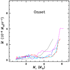
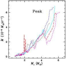
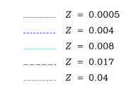
Figure 1: Superwind phase fiducial mass-loss rate, $\dot{M}$, versus zero-age main-sequence stellar mass, $M_{\rm i}$. Left: onset stage; right: peak stage. Black dotted line: $Z=$ 0.0005; blue short-dashed line: $Z=$ 0.004; cyan solid line: $Z=$ 0.008; red long-dashed line: $Z=$ 0.017; magenta dotted-short-dashed line: $Z=$ 0.04.

For this work, I adopt the view (e.g., Willson, 2000) that empirical relations between mass-loss and stellar parameters are the result of very strong selection effects, since stars with a low rate will not be detected as mass-losing, whereas stars with a high rate will be obscured by dust and/or extremely short-lived. In other words, regardless of the actual rate, mass-loss will appear to follow a Reimers’ type relation (Reimers, 1975, 1977), $\dot{M}=\eta LR/M$, where $M$ and $L$ are, respectively, the stellar mass and luminosity, $R(L,M,Z)$ is the stellar radius, and $\eta$ is a fitting parameter. Moreover, mass-loss is not a smooth process: as $\dot{M}$ increases, $L$ first grows, while $M$ stays constant, until the stellar configuration reaches a ‘cliff’ in the log $M$ versus log $L$ plane; subsequently, mass-loss depends on stellar parameters much more steeply than implied by empirical relations, and the stellar envelope is shed in an extremely short time at roughly constant $L$.

Consequently, rather than, for example, varying $\eta$ while leaving the stellar parameters unchanged, I will vary together the mass-loss rate and the stellar parameters, in a consistent fashion. The whole procedure has been described in detail in Appendix A1 of González-Lópezlira et al. (2010).

Briefly, $\dot{M}$ (computed from the mass differences along the track for a given star) is treated as the independent parameter. When $\dot{M}$ is changed with respect to its fiducial value, a modified stellar luminosity $L$ and a modified stellar radius $R$ are obtained, respectively, from Fig. 2 in Bowen & Willson (1991) and eq. 4 in Iben (1984). A new effective temperature is derived using $L=R^{2}(T_{\rm eff}/5770)^{4}$. The lifetimes $t$ within each of the superwind stages are then adjusted according to the fuel-consumption theorem (Renzini & Buzzoni, 1986), i.e., assuming that the product $Lt$ is constant (and equal to the value for fiducial $\dot{M}$) for each star and stage. If the product $\dot{M}t$ exceeds the stellar mass at the beginning of a stage, the star will not reach the following stage. Fundamental mode pulsation periods, which change with stellar configuration, and C/O ratios of C-rich stars, which vary with $\dot{M}$, are modified according to, respectively, eq. (12) and eq. (23) in Marigo & Girardi (2007).

The effects of dust on the stellar SEDs are included as explained in Appendix A2 of González-Lópezlira et al. (2010), following a procedure outlined by Piovan et al. (2003) and Marigo et al. (2008). Summing up, the optical depth at wavelength $\lambda$, $\tau_{\lambda}$, is proportional to $\dot{M}\Psi\kappa_{\lambda}v_{\rm exp}^{-1}L^{-0.5}$, where $\Psi$ is the dust-to-gas ratio, $\kappa_{\lambda}$ is the mass extinction coefficient, and $v_{\rm exp}$ is the wind expansion velocity. However, both $v_{\rm exp}$ and $\kappa_{\lambda}$ are functions of $\dot{M}$ (the latter through dust composition), and thus $\tau_{\lambda}$ must be found through an iterative process. If $\Psi$ and hence $\tau$ diverge (González-Lópezlira et al. 2010, eqs. (A17) and (A3)), the star in question will be invisible during the corresponding stage.

Finally, to produce the output SEDs of the TP-AGB stars, the radiative transfer in their dusty envelopes is calculated with the software DUSTY, as reported in Appendix A3 of González-Lópezlira et al. (2010). Dust mixtures for C-rich and O-rich stars with varying envelope optical depths are adopted from Suh (1999, 2000, 2002).

CB^∗ models with fiducial mass-loss are reported in Tables 2 and 3: mid-IR colors as a function of age, for different metallicities, are presented in Table 2; fluctuation amplitudes are listed in Table 3.

Table 2: IR Colors for CB^∗ Models with Fiducial Mass-loss

Age (Gyr)	$[V-3.6]$	$[3.6-4.5]$	$[4.5-5.8]$	$[5.8-8]$	$[8-24]$
$Z=0.017\ \ Y=0.279$
0.005	2.110	-0.068	0.045	0.110	-0.428
0.006	2.541	-0.065	0.048	0.118	-0.419
0.007	3.674	0.095	0.079	0.086	-0.330
0.008	3.515	0.094	0.079	0.085	-0.331
0.009	3.192	0.091	0.077	0.084	-0.334
0.010	2.389	0.084	0.073	0.081	-0.340
0.020	2.590	0.060	0.070	0.085	-0.353
0.030	1.935	0.002	0.059	0.092	-0.387
0.040	1.707	-0.033	0.050	0.094	-0.413
0.050	1.614	-0.056	0.045	0.095	-0.429
0.060	1.602	-0.068	0.042	0.096	-0.438
0.070	1.699	-0.062	0.045	0.094	-0.431
0.080	1.666	-0.066	0.042	0.091	-0.437
0.090	2.309	0.149	0.213	0.755	1.697
0.100	2.370	0.109	0.187	0.725	1.600
0.200	2.308	0.084	0.184	0.571	1.520
0.300	2.250	0.188	0.394	0.639	0.940
0.400	2.287	0.176	0.370	0.589	0.872
0.500	2.395	0.203	0.339	0.500	0.703
0.600	2.412	0.196	0.337	0.512	0.753
0.700	2.557	0.194	0.312	0.450	0.544
0.800	2.594	0.180	0.291	0.418	0.476
0.900	2.626	0.164	0.269	0.382	0.394
1.000	2.603	0.137	0.283	0.444	0.640
1.500	2.675	0.057	0.180	0.232	0.096
2.000	2.926	-0.058	0.059	0.227	0.429
3.000	3.145	-0.025	0.045	0.180	0.202
4.000	3.036	-0.030	0.044	0.157	0.067
5.000	3.111	-0.029	0.049	0.147	0.000
6.000	3.071	-0.026	0.044	0.143	-0.019
7.000	3.091	-0.025	0.044	0.144	-0.004
8.000	3.116	-0.023	0.052	0.140	-0.032
9.000	3.130	-0.023	0.054	0.128	-0.121
10.000	3.170	-0.023	0.056	0.123	-0.156
11.000	3.190	-0.018	0.055	0.133	-0.086
12.000	3.205	-0.016	0.056	0.128	-0.123
13.000	3.231	-0.016	0.058	0.126	-0.137
13.500	3.243	-0.016	0.059	0.123	-0.153

Note. Values for solar metallicity and helium content are shown here for guidance regarding the table’s form and content. (This table is available in its entirety in machine-readable form.)

Table 3: SBF Amplitudes for CB^∗ Models with Fiducial Mass-loss

Age (Gyr)	$\mbox{$\bar{M}$}_{3.6}$	$\mbox{$\bar{M}$}_{4.5}$	$\mbox{$\bar{M}$}_{5.8}$	$\mbox{$\bar{M}$}_{8}$	$\mbox{$\bar{M}$}_{24}$
$Z=0.017\ \ Y=0.279$
0.005	-11.795	-11.722	-11.775	-11.899	-11.484
0.006	-11.281	-11.238	-11.295	-11.412	-11.015
0.007	-11.596	-11.693	-11.776	-11.864	-11.539
0.008	-11.105	-11.203	-11.285	-11.373	-11.048
0.009	-10.740	-10.836	-10.917	-11.006	-10.680
0.010	-10.402	-10.497	-10.582	-10.674	-10.353
0.020	-9.231	-9.315	-9.396	-9.488	-9.159
0.030	-8.408	-8.488	-8.573	-8.670	-8.349
0.040	-7.839	-7.899	-7.987	-8.092	-7.771
0.050	-7.448	-7.494	-7.582	-7.694	-7.372
0.060	-7.221	-7.260	-7.349	-7.464	-7.141
0.070	-7.622	-7.758	-7.875	-7.983	-7.740
0.080	-7.353	-7.484	-7.599	-7.706	-7.459
0.090	-9.595	-10.227	-10.699	-11.978	-14.212
0.100	-9.534	-10.107	-10.564	-11.863	-14.102
0.200	-8.873	-9.510	-10.035	-11.379	-13.920
0.300	-8.611	-9.851	-11.128	-12.366	-13.695
0.400	-8.363	-9.474	-10.721	-12.004	-13.418
0.500	-8.533	-9.549	-10.535	-11.705	-13.227
0.600	-8.419	-9.474	-10.475	-11.670	-13.304
0.700	-8.319	-9.430	-10.371	-11.386	-12.589
0.800	-8.275	-9.354	-10.246	-11.206	-12.333
0.900	-8.229	-9.273	-10.110	-11.009	-12.044
1.000	-7.985	-8.968	-9.941	-11.165	-12.800
1.500	-7.771	-8.634	-9.265	-9.945	-10.703
2.000	-6.939	-7.008	-7.095	-8.215	-10.699
3.000	-6.482	-6.568	-6.595	-7.569	-10.195
4.000	-6.281	-6.342	-6.335	-7.059	-9.344
5.000	-6.146	-6.203	-6.223	-6.859	-9.013
6.000	-6.096	-6.168	-6.148	-6.760	-8.872
7.000	-6.076	-6.178	-6.178	-6.953	-9.580
8.000	-5.931	-6.034	-6.070	-6.726	-9.082
9.000	-5.810	-5.907	-5.957	-6.437	-8.384
10.000	-5.767	-5.868	-5.929	-6.327	-8.041
11.000	-5.799	-5.930	-5.989	-6.566	-8.865
12.000	-5.761	-5.910	-5.975	-6.574	-9.040
13.000	-5.743	-5.894	-5.970	-6.513	-8.889
13.500	-5.734	-5.885	-5.964	-6.476	-8.814

Note. Values for solar metallicity and helium content are shown here for guidance regarding the table’s form and content. (This table is available in its entirety in machine-readable form.)

3 Broadband Colors.

3.1 Individual AGB Stars.

I show theoretical color-color diagrams of individual TP-AGB stars along the 0.2 Gyr (dotted line), 0.5 Gyr (solid line), and 9.5 Gyr (dashed line) isochrones, for populations with four metallicities ($Z=$ 0.004, black; 0.008, cyan; 0.017, red; and 0.04, magenta) and five choices of spectra; these vary only due to the mass-loss rate adopted for stars in the TP-AGB. Figure 2 displays, from left to right, fiducial $\dot{M}/10$, fiducial $\dot{M}/2$, fiducial $\dot{M}$, fiducial $\dot{M}\times 5$, fiducial $\dot{M}\times 10$. The top and bottom rows present, respectively, [5.8 - 8] versus [3.6 - 4.5] and [8 - 24] versus [3.6 - 8].

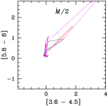
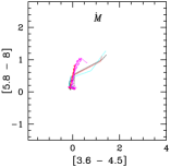
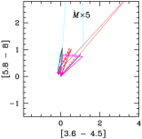
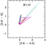
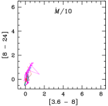
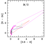
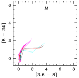
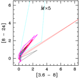
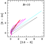
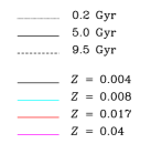
Figure 2: Theoretical two-color diagrams of individual TP-AGB stars along the 0.2 Gyr (dotted line), 5.0 Gyr (solid line), and 9.5 Gyr (dashed line) isochrones. Top row: [5.8 - 8] versus [3.6 - 4.5]; bottom row: [8 - 24] versus [3.6 - 8]. From left to right: fiducial $\dot{M}/10$, fiducial $\dot{M}/2$, fiducial $\dot{M}$, fiducial $\dot{M}\times 5$, fiducial $\dot{M}\times 10$. Different colors indicate diverse metallicities, i.e., black: $Z$ = 0.004; cyan: $Z$ = 0.008; red: $Z$ = 0.017; magenta: $Z$ = 0.04.

As a first test, I compare the model mid-IR broadband colors to the observed [5.8 - 8] versus [3.6 - 4.5] and [8 - 24] versus [3.6 - 8] color-color diagrams of individual AGB stars in the sample published by Srinivasan et al. (2009). In Figure 3, different colors are used for O-rich, C-rich, and “extreme” (based on their near- and mid-IR colors) AGB objects. Next, in Figure 4, models with both fiducial (thick lines) and 10 $\times$ fiducial (thin lines) mass-loss rates are superimposed on the stars, shown as a cloud of gray points. The ages and metallicities of the models are indicated as in Figure 2. The reddest extreme AGB stars are not fitted by models with fiducial $\dot{M}$.

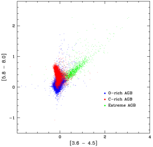
Figure 3: Integrated mid-IR colors of individual AGB candidates in the sample of Srinivasan et al. (2009). Blue: O-rich stars. Red: C-rich stars. Green: “extreme” AGB stars; these are the most luminous AGB stars, losing the most mass. Left: [5.8 - 8] versus [3.6 - 4.5]; right: [8 - 24] versus [3.6 - 8]. For a 10th mag star at [8], typical photometric errors are 0.15 mag at [3.6], 0.10 mag at [8], and 0.12 mag at [24]. Some extreme stars, however, can have errors of up to 0.15 mag in the IRAC bands, despite being brighter.

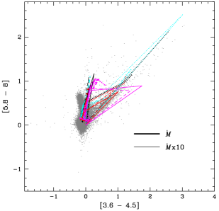
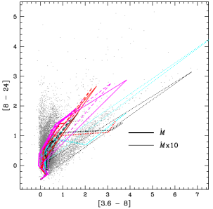
Figure 4: Superimposed on the sample of observed AGB stars, now shown as gray points, theoretical mid-IR colors of individual TP-AGB stars along isochrones of populations with different mass-loss rates and metallicities. Left: [5.8 - 8] versus [3.6 - 4.5]; right: [8 - 24] versus [3.6 - 8]. Thick lines: fiducial mass-loss rate $\dot{M}$; thin lines: high mass-loss rate $\dot{M}\times$ 10. Metallicities and isochrone ages indicated as in Fig. 2.

3.2 Star Clusters.

Figure 5 presents theoretical two-color diagrams, [5.8 - 8] versus [3.6 - 4.5] and [8 - 24] versus [3.6 - 8], for SSPs with different metallicities ($Z$ = 0.0005, blue; 0.008, cyan; 0.017, red) and, again, our five choices of mass-loss and spectra for stars in the TP-AGB ($\dot{M}/10$, $\dot{M}/2$, $\dot{M}$, $\dot{M}\times 5$, and $\dot{M}\times 10$). The model ages go from 10 Myr to 14 Gyr. Differing from models and observed colors of individual stars (see Figures 2 and 4), the integrated colors of SSP models are confined to the smaller parameter space -0.1 $\lesssim$ [3.6 - 4.5] $\lesssim$ 0.5, 0. $\lesssim$ [5.8 - 8] $\lesssim$ 1.5, regardless of mass-loss rate. On the other hand, the expected [8 - 24] versus [3.6 - 8] colors of SSPs occupy ranges similar to those of single stars.

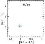
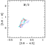
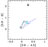
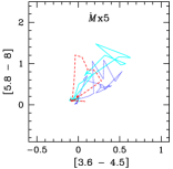
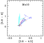
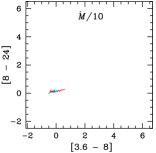
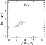
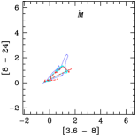
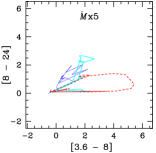
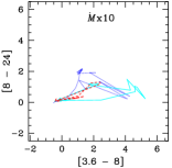
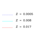
Figure 5: Theoretical two-color diagrams for SSPs with different metallicities and mass-loss rates in the TP-AGB. Top row: [5.8 - 8] versus [3.6 - 4.5]; bottom row: [8 - 24] versus [3.6 - 8]. From left to right: fiducial $\dot{M}/10$, fiducial $\dot{M}/2$, fiducial $\dot{M}$, fiducial $\dot{M}\times 5$, fiducial $\dot{M}\times 10$. Models span an age range between 10 Myr and 14 Gyr. Blue dotted line: $Z$ = 0.0005; cyan solid line: $Z$ = 0.008; red dashed line: $Z$ = 0.017.

For comparison with the models, I use data from the Spitzer Space Telescope surveys of the LMC and SMC: SAGE (Meixner et al., 2006; Meixner, 2008) and SAGE-SMC (Gordon et al., 2011), respectively. SAGE consists in a uniform imaging survey of the LMC with the four IRAC channels (i.e., [3.6], [4.5], [5.8], and [8]), and the three Multiband Imaging Photometer (MIPS) bands ([24], [70], and [160]); I only use the IRAC and MIPS [24] data in this work. The surveyed area was $7\fdg 1\times 7\fdg 1$ with IRAC and $7\fdg 8\times 7\fdg 8$ with MIPS.

All four IRAC detectors are 256² pixels in size; the pixels are $1\farcs 22\times 1\farcs 22$, for a $5\farcm 2\times 5\farcm 2$ field of view (FOV). The two shorter wavelength channels employ InSb detectors, whereas at [5.8] and [8] the camera works with Si:As impurity band conduction (IBC) arrays. The actual angular resolution of the survey is $1\farcs 7,1\farcs 7,1\farcs 9$ and $2\arcsec$, respectively, at [3.6], [4.5], [5.8], and [8]. The minimum effective exposure time per pixel in each channel was 43 s. The 5$\sigma$ point-source sensitivity attained is 17 mag at [3.6], 16 mag at [4.5], 14 mag at [5.8], and 13.5 mag at [8]. For 24 $\mu$m imaging, the MIPS has a 128² pixel Si:As IBC array. The pixels are $2\farcs 5\times 2\farcs 5$ in size, for a $5\arcmin\times 5\arcmin$ FOV. The angular resolution of the 24 $\mu$m survey is $6\arcsec$. The minimum effective exposure time per pixel was 60 s, with a 5$\sigma$ point-source sensitivity of 10.4 mag.

SAGE-LMC covers an area of $\sim 30$ deg². Effective exposure times per pixel were 42 s for IRAC and 60 s for MIPS. The angular resolutions of the images are 2$\arcsec$ for IRAC and 6$\arcsec$ for MIPS at [24]. The 5$\sigma$ point-source sensitivity is 17 mag, 17 mag, 15 mag, 14.5 mag, and 10 mag, respectively, at [3.6], [4.5], [5.8], [8], and [24].

I have measured in the SAGE mosaics the integrated magnitudes of the LMC and SMC clusters listed in Table 4. Clusters that had visible nebulosity at [8] were not included in our sample. The measurements were performed in apertures with $r=$ 1 arcmin, while the contributions of the sky and the field were estimated in an annulus with 2$\farcm$0 $<r\leq$ 2$\farcm$5 and subtracted. Although not very important, a reddening correction was also applied. $E(B-V)$ values were taken from Persson et al. (1983) for individual clusters; when these were not available, we assumed $E(B-V)=0.075$ and $E(B-V)=0.037$, respectively, for the LMC and SMC (Schlegel et al., 1998). Table 4 shows the cluster names, cloud membership, and integrated magnitudes at [3.6], [4.5], [5.8], [8], and [24]. Integrated magnitudes are missing either because the clusters were not imaged by the survey (mainly at [24]), or because they contained very prominent interstellar nebulosity. The clusters are grouped by SWB class (Searle et al., 1980), including a very young pre-SWB category (González et al., 2004; González-Lópezlira et al., 2005, 2010).

Table 4: Individual Cluster Photometry

			[3.6]	[4.5]	[5.8]	[8]	[24]
Supercluster	Name	Cloud	mag	mag	mag	mag	mag
Pre-SWB	L 84	SMC	11.30 $\pm$ 0.10	11.03 $\pm$ 0.09	9.83 $\pm$ 0.07	8.38 $\pm$ 0.04	…
	L 107	SMC	11.51 $\pm$ 0.09	11.63 $\pm$ 0.10	11.25 $\pm$ 0.11	10.80 $\pm$ 0.12	…
	NGC 602	SMC	10.86 $\pm$ 0.05	10.39 $\pm$ 0.06	9.36 $\pm$ 0.05	7.99 $\pm$ 0.03	…
	NGC 1983	LMC	7.39 $\pm$ 0.01	7.23 $\pm$ 0.01	6.49 $\pm$ 0.01	6.00 $\pm$ 0.01	4.18 $\pm$ 0.04
	NGC 1984	LMC	7.13 $\pm$ 0.01	6.73 $\pm$ 0.01	5.44 $\pm$ 0.01	4.10 $\pm$ 0.01	-0.669 $\pm$0.004
	NGC 2001	LMC	8.37 $\pm$ 0.02	8.46 $\pm$ 0.02	7.34 $\pm$ 0.02	7.49 $\pm$ 0.02	5.98 $\pm$ 0.08
	NGC 2006	LMC	8.70 $\pm$ 0.02	8.73 $\pm$ 0.03	8.58 $\pm$ 0.03	8.69 $\pm$ 0.05	…
	NGC 2011	LMC	7.48 $\pm$ 0.01	7.44 $\pm$ 0.01	6.86 $\pm$ 0.02	…	…
	NGC 2014	LMC	7.14 $\pm$ 0.01	7.01 $\pm$ 0.01	5.05 $\pm$ 0.01	3.515 $\pm$ 0.005	…
	NGC 2027	LMC	8.33 $\pm$ 0.02	7.83 $\pm$ 0.02	7.08 $\pm$ 0.02	6.80 $\pm$ 0.02	6.23 $\pm$ 0.08
	SL 114	LMC	9.40 $\pm$ 0.03	9.19 $\pm$ 0.03	8.53 $\pm$ 0.04	7.31 $\pm$ 0.03	5.57 $\pm$ 0.07
SWB I	L 45	SMC	9.63 $\pm$ 0.02	9.63 $\pm$ 0.03	9.13 $\pm$ 0.04	8.57 $\pm$ 0.04	…
	L 51	SMC	8.98 $\pm$ 0.02	8.84 $\pm$ 0.02	8.57 $\pm$ 0.04	8.59 $\pm$ 0.04	…
	L 56	SMC	11.15 $\pm$ 0.11	11.06 $\pm$ 0.12	10.28 $\pm$ 0.06	9.95 $\pm$ 0.08	…
	L 66	SMC	10.64 $\pm$ 0.02	10.74 $\pm$ 0.04	10.64 $\pm$ 0.04	10.80 $\pm$ 0.09	…
	NGC 290	SMC	10.13 $\pm$ 0.05	10.37 $\pm$ 0.07	9.72 $\pm$ 0.05	…	…
	NGC 299	SMC	9.07 $\pm$ 0.02	9.21 $\pm$ 0.02	8.88 $\pm$ 0.03	8.87 $\pm$ 0.05	…
	NGC 330	SMC	7.95 $\pm$ 0.02	8.09 $\pm$ 0.02	7.75 $\pm$ 0.02	7.66 $\pm$ 0.03	…
	NGC 376	SMC	8.76 $\pm$ 0.02	8.92 $\pm$ 0.02	8.61 $\pm$ 0.03	8.63 $\pm$ 0.05	…
	NGC 1704	LMC	9.06 $\pm$ 0.02	9.23 $\pm$ 0.03	9.16 $\pm$ 0.04	…	…
	NGC 1711	LMC	8.13 $\pm$ 0.02	8.18 $\pm$ 0.02	7.96 $\pm$ 0.02	7.96 $\pm$ 0.03	7.99 $\pm$ 0.31
	NGC 1787	LMC	8.06 $\pm$ 0.02	8.19 $\pm$ 0.02	7.91 $\pm$ 0.02	7.81 $\pm$ 0.03	7.50 $\pm$ 0.16
	NGC 1805	LMC	8.03 $\pm$ 0.02	7.51 $\pm$ 0.01	6.87 $\pm$ 0.01	6.47 $\pm$ 0.02	4.73 $\pm$ 0.04
	NGC 1810	LMC	8.88 $\pm$ 0.02	9.10 $\pm$ 0.03	9.10 $\pm$ 0.04	9.24 $\pm$ 0.08	…
	NGC 1818	LMC	7.12 $\pm$ 0.01	7.26 $\pm$ 0.01	6.98 $\pm$ 0.01	6.97 $\pm$ 0.02	…
	NGC 2002	LMC	6.89 $\pm$ 0.01	6.86 $\pm$ 0.01	6.09 $\pm$ 0.01	5.83 $\pm$ 0.01	4.32 $\pm$ 0.04
	NGC 2003	LMC	9.05 $\pm$ 0.02	9.27 $\pm$ 0.03	9.00 $\pm$ 0.04	9.06 $\pm$ 0.05	8.73 $\pm$ 0.42
	NGC 2004	LMC	6.30 $\pm$ 0.01	6.41 $\pm$ 0.01	5.94 $\pm$ 0.01	5.72 $\pm$ 0.01	…
	NGC 2009	LMC	7.36 $\pm$ 0.01	7.02 $\pm$ 0.01	6.13 $\pm$ 0.01	5.39 $\pm$ 0.01	…
	NGC 2098	LMC	8.11 $\pm$ 0.02	8.29 $\pm$ 0.02	8.04 $\pm$ 0.03	8.33 $\pm$ 0.05	…
	NGC 2100	LMC	6.11 $\pm$ 0.01	6.20 $\pm$ 0.01	5.73 $\pm$ 0.01	5.74 $\pm$ 0.01	…
	NGC l477	LMC	8.94 $\pm$ 0.02	9.18 $\pm$ 0.03	9.19 $\pm$ 0.05	9.78 $\pm$ 0.15	…
	NGC l538	LMC	8.69 $\pm$ 0.02	8.78 $\pm$ 0.03	8.36 $\pm$ 0.03	8.39 $\pm$ 0.04	…
SWB II	IC 1624	SMC	9.22 $\pm$ 0.02	9.31 $\pm$ 0.02	8.97 $\pm$ 0.03	8.92 $\pm$ 0.02	…
	IC 1655	SMC	13.04 $\pm$ 0.23	13.14 $\pm$ 0.24	…	12.53 $\pm$ 0.33	…
	NGC 220	SMC	10.88 $\pm$ 0.06	11.05 $\pm$ 0.10	10.74 $\pm$ 0.10	10.75 $\pm$ 0.13	…
	NGC 222	SMC	9.42 $\pm$ 0.03	9.51 $\pm$ 0.03	9.23 $\pm$ 0.04	9.33 $\pm$ 0.04	…
	NGC 231	SMC	11.07 $\pm$ 0.06	11.19 $\pm$ 0.11	11.29 $\pm$ 0.11	11.04 $\pm$ 0.14	…
	NGC 242	SMC	9.60 $\pm$ 0.03	9.72 $\pm$ 0.05	9.55 $\pm$ 0.05	9.30 $\pm$ 0.07	…
	NGC 422	SMC	11.91 $\pm$ 0.12	12.22 $\pm$ 0.17	11.90 $\pm$ 0.17	…	…
	NGC 1732	LMC	9.67 $\pm$ 0.04	9.39 $\pm$ 0.04	8.82 $\pm$ 0.04	7.60 $\pm$ 0.03	6.02 $\pm$ 0.07
	NGC 1735	LMC	8.68 $\pm$ 0.02	8.70 $\pm$ 0.03	8.13 $\pm$ 0.03	7.30 $\pm$ 0.03	…
	NGC 1755	LMC	8.05 $\pm$ 0.02	8.20 $\pm$ 0.02	7.91 $\pm$ 0.02	7.87 $\pm$ 0.04	6.89 $\pm$ 0.17
	NGC 1774	LMC	8.27 $\pm$ 0.02	8.55 $\pm$ 0.02	8.29 $\pm$ 0.03	9.36 $\pm$ 0.07	…
	NGC 1782	LMC	7.45 $\pm$ 0.01	7.60 $\pm$ 0.02	7.28 $\pm$ 0.02	7.20 $\pm$ 0.03	…
	NGC 1793	LMC	9.34 $\pm$ 0.03	9.38 $\pm$ 0.04	9.37 $\pm$ 0.06	…	6.65 $\pm$ 0.15
	NGC 1834	LMC	8.57 $\pm$ 0.02	8.74 $\pm$ 0.03	8.73 $\pm$ 0.04		7.60 $\pm$ 0.20
	NGC 1847	LMC	7.75 $\pm$ 0.01	7.70 $\pm$ 0.02	7.29 $\pm$ 0.02	6.90 $\pm$ 0.03	…
	NGC 1854	LMC	7.90 $\pm$ 0.02	8.05 $\pm$ 0.02	…	…	…
	NGC 1863	LMC	9.12 $\pm$ 0.03	…	…	…	…
	NGC 1870	LMC	8.97 $\pm$ 0.03	9.15 $\pm$ 0.03	8.61 $\pm$ 0.04	7.45 $\pm$ 0.04	…
	NGC 1928	LMC	8.13 $\pm$ 0.02	8.37 $\pm$ 0.02	8.45 $\pm$ 0.04	…	…
	NGC 1951	LMC	8.52 $\pm$ 0.02	8.53 $\pm$ 0.02	8.09 $\pm$ 0.02	8.04 $\pm$ 0.04	6.74 $\pm$ 0.15
	NGC 2118	LMC	8.87 $\pm$ 0.02	9.04 $\pm$ 0.03	8.77 $\pm$ 0.04	8.00 $\pm$ 0.05	…
	NGC 2164	LMC	9.00 $\pm$ 0.02	8.90 $\pm$ 0.03	8.70 $\pm$ 0.03	8.67 $\pm$ 0.04	8.13 $\pm$ 0.30
	SL 56	LMC	10.07 $\pm$ 0.04	9.80 $\pm$ 0.04	9.38 $\pm$ 0.05	9.60 $\pm$ 0.07	9.37 $\pm$ 0.82
	SL 106	LMC	9.44 $\pm$ 0.03	9.46 $\pm$ 0.04	9.07 $\pm$ 0.04	…	…
SWB III	IC 1611	SMC	10.37 $\pm$ 0.04	10.51 $\pm$ 0.04	10.08 $\pm$ 0.09	10.17 $\pm$ 0.16	…
	L 40	SMC	9.55 $\pm$ 0.03	9.72 $\pm$ 0.04	9.54 $\pm$ 0.05	9.82 $\pm$ 0.08	…
	L 44	SMC	9.56 $\pm$ 0.02	9.59 $\pm$ 0.03	9.28 $\pm$ 0.06	9.03 $\pm$ 0.05	…
	L 63	SMC	…	…	10.84 $\pm$ 0.12	11.09 $\pm$ 0.33	…
	L 114	SMC	10.77 $\pm$ 0.06	10.88 $\pm$ 0.07	10.61 $\pm$ 0.09	10.80 $\pm$ 0.19	…
	NGC 265	SMC	10.23 $\pm$ 0.03	10.32 $\pm$ 0.03	9.78 $\pm$ 0.07	8.89 $\pm$ 0.05	…
	NGC 458	SMC	10.69 $\pm$ 0.05	10.81 $\pm$ 0.07	10.65 $\pm$ 0.09	10.53 $\pm$ 0.11	…
	NGC 1844	LMC	9.94 $\pm$ 0.04	10.03 $\pm$ 0.05	9.63 $\pm$ 0.04	9.22 $\pm$ 0.06	7.73 $\pm$ 0.02
	NGC 1866	LMC	7.29 $\pm$ 0.01	7.47 $\pm$ 0.01	7.12 $\pm$ 0.02	7.13 $\pm$ 0.02	6.90 $\pm$ 0.14
	NGC 1895	LMC	8.79 $\pm$ 0.02	8.50 $\pm$ 0.02	6.59 $\pm$ 0.01	5.03 $\pm$ 0.01	2.33 $\pm$ 0.01
	NGC 1953	LMC	8.91 $\pm$ 0.02	8.90 $\pm$ 0.03	8.61 $\pm$ 0.05	…	…
	NGC 2000	LMC	9.43 $\pm$ 0.03	9.58 $\pm$ 0.04	9.56 $\pm$ 0.05	10.25 $\pm$ 0.08	…
	NGC 2025	LMC	9.15 $\pm$ 0.03	9.10 $\pm$ 0.03	8.93 $\pm$ 0.04	9.13 $\pm$ 0.06	8.51 $\pm$ 0.46
	NGC 2031	LMC	8.15 $\pm$ 0.02	8.52 $\pm$ 0.02	7.69 $\pm$ 0.02	8.38 $\pm$ 0.03	7.62 $\pm$ 0.20
	NGC 2134	LMC	8.40 $\pm$ 0.02	8.54 $\pm$ 0.02	8.19 $\pm$ 0.03	8.26 $\pm$ 0.04	7.93 $\pm$ 0.08
	NGC 2136	LMC	8.14 $\pm$ 0.02	8.30 $\pm$ 0.02	7.94 $\pm$ 0.02	7.97 $\pm$ 0.03	7.20 $\pm$ 0.13
	NGC 2156	LMC	9.96 $\pm$ 0.04	10.07 $\pm$ 0.05	10.03 $\pm$ 0.08	9.73 $\pm$ 0.04	7.74 $\pm$ 0.18
	NGC 2157	LMC	8.11 $\pm$ 0.02	8.24 $\pm$ 0.02	7.98 $\pm$ 0.02	7.96 $\pm$ 0.03	7.66 $\pm$ 0.23
	NGC 2159	LMC	9.56 $\pm$ 0.03	9.64 $\pm$ 0.04	9.37 $\pm$ 0.04	9.56 $\pm$ 0.04	9.73 $\pm$ 0.85
	NGC 2172	LMC	10.02 $\pm$ 0.04	10.21 $\pm$ 0.05	9.78 $\pm$ 0.04	10.18 $\pm$ 0.05	…
	NGC l539	LMC	7.64 $\pm$ 0.01	7.89 $\pm$ 0.02	7.56 $\pm$ 0.02	7.59 $\pm$ 0.03	…
SWB IV	L 26	SMC	11.22 $\pm$ 0.09	11.37 $\pm$ 0.10	11.36 $\pm$ 0.13	10.98 $\pm$ 0.15	…
	L 53	SMC	10.14 $\pm$ 0.04	10.20 $\pm$ 0.05	9.85 $\pm$ 0.06	9.66 $\pm$ 0.08	…
	NGC 294	SMC	9.96 $\pm$ 0.04	10.09 $\pm$ 0.03	9.97 $\pm$ 0.08	9.99 $\pm$ 0.14	…
	NGC 1801	LMC	8.32 $\pm$ 0.02	8.48 $\pm$ 0.02	8.23 $\pm$ 0.03	8.13 $\pm$ 0.04	…
	NGC 1831	LMC	8.27 $\pm$ 0.02	8.40 $\pm$ 0.02	8.11 $\pm$ 0.02	7.92 $\pm$ 0.03	8.07 $\pm$ 0.21
	NGC 1849	LMC	8.47 $\pm$ 0.02	8.28 $\pm$ 0.02	7.83 $\pm$ 0.02	7.37 $\pm$ 0.02	6.60 $\pm$ 0.12
	NGC 1868	LMC	9.17 $\pm$ 0.03	9.44 $\pm$ 0.04	9.25 $\pm$ 0.04	9.06 $\pm$ 0.05	…
	NGC 1987	LMC	8.43 $\pm$ 0.02	8.53 $\pm$ 0.02	8.33 $\pm$ 0.03	8.41 $\pm$ 0.04	9.65 $\pm$ 0.61
	NGC 2056	LMC	9.07 $\pm$ 0.03	9.12 $\pm$ 0.03	8.73 $\pm$ 0.04	…	…
	NGC 2107	LMC	8.61 $\pm$ 0.02	8.63 $\pm$ 0.03	8.25 $\pm$ 0.03	7.88 $\pm$ 0.04	…
SWB V	NGC 152	SMC	9.41 $\pm$ 0.03	9.60 $\pm$ 0.04	9.28 $\pm$ 0.04	9.05 $\pm$ 0.05	…
	NGC 411	SMC	9.55 $\pm$ 0.03	9.65 $\pm$ 0.04	9.34 $\pm$ 0.04	9.20 $\pm$ 0.05	…
	NGC 419	SMC	7.51 $\pm$ 0.01	7.51 $\pm$ 0.02	6.90 $\pm$ 0.01	6.36 $\pm$ 0.01	…
	NGC 1651	LMC	8.75 $\pm$ 0.02	8.93 $\pm$ 0.03	8.61 $\pm$ 0.03	8.53 $\pm$ 0.05	8.21 $\pm$ 0.23
	NGC 1783	LMC	7.49 $\pm$ 0.01	7.65 $\pm$ 0.02	7.24 $\pm$ 0.02	6.99 $\pm$ 0.02	…
	NGC 1795	LMC	9.27 $\pm$ 0.03	9.55 $\pm$ 0.04	9.35 $\pm$ 0.05	9.13 $\pm$ 0.06	8.08 $\pm$ 0.29
	NGC 1846	LMC	6.91 $\pm$ 0.01	7.13 $\pm$ 0.01	6.84 $\pm$ 0.01	6.59 $\pm$ 0.02	6.56 $\pm$ 0.09
	NGC 1917	LMC	8.80 $\pm$ 0.02	…	…	…	…
	NGC 2154	LMC	8.15 $\pm$ 0.02	8.39 $\pm$ 0.02	8.16 $\pm$ 0.03	7.85 $\pm$ 0.03	7.58 $\pm$ 0.25
SWB VI	NGC 416	SMC	9.29 $\pm$ 0.03	9.41 $\pm$ 0.03	9.13 $\pm$ 0.04	9.18 $\pm$ 0.05	8.94 $\pm$ 0.09
	NGC 1751	LMC	7.76 $\pm$ 0.01	7.96 $\pm$ 0.02	7.79 $\pm$ 0.02	7.55 $\pm$ 0.03	…
	NGC 1754	LMC	7.93 $\pm$ 0.01	7.98 $\pm$ 0.02	7.65 $\pm$ 0.02	7.53 $\pm$ 0.03	6.90 $\pm$ 0.11
	NGC 1852	LMC	8.09 $\pm$ 0.02	8.18 $\pm$ 0.02	7.76 $\pm$ 0.02	6.96 $\pm$ 0.02	3.29 $\pm$ 0.02
	NGC 1916	LMC	6.86 $\pm$ 0.01	6.96 $\pm$ 0.01	5.80 $\pm$ 0.01	4.44 $\pm$ 0.01	…
	NGC 1978	LMC	6.79 $\pm$ 0.01	6.72 $\pm$ 0.01	6.14 $\pm$ 0.01	5.72 $\pm$ 0.01	…
	NGC 2005	LMC	8.42 $\pm$ 0.02	8.63 $\pm$ 0.03	8.26 $\pm$ 0.03	8.29 $\pm$ 0.05	…
	NGC 2019	LMC	7.94 $\pm$ 0.02	8.14 $\pm$ 0.02	7.90 $\pm$ 0.02	7.84 $\pm$ 0.05	…
	NGC 2121	LMC	8.05 $\pm$ 0.02	8.08 $\pm$ 0.02	7.70 $\pm$ 0.02	7.51 $\pm$ 0.03	7.31 $\pm$ 0.19
	SL 506	LMC	10.56 $\pm$ 0.05	10.68 $\pm$ 0.07	10.42 $\pm$ 0.09	10.22 $\pm$ 0.04	9.16 $\pm$ 0.41
SWB VII	L 8	SMC	…	…	…	9.60 $\pm$ 0.05	…
	L 11	SMC	10.66 $\pm$ 0.05	10.81 $\pm$ 0.06	10.75 $\pm$ 0.09	10.26 $\pm$ 0.10	…
	L 68	SMC	…	…	10.55 $\pm$ 0.07	10.66 $\pm$ 0.21	…
	L 113	SMC	10.37 $\pm$ 0.03	10.51 $\pm$ 0.05	10.22 $\pm$ 0.05	9.97 $\pm$ 0.08	…
	NGC 339	SMC	10.40 $\pm$ 0.06	10.44 $\pm$ 0.06	10.26 $\pm$ 0.06	10.19 $\pm$ 0.10	…
	NGC 361	SMC	9.85 $\pm$ 0.04	10.00 $\pm$ 0.05	9.73 $\pm$ 0.05	9.71 $\pm$ 0.08	…
	NGC 1786	LMC	7.74 $\pm$ 0.01	7.76 $\pm$ 0.02	7.48 $\pm$ 0.02	7.32 $\pm$ 0.02	6.75 $\pm$ 0.14
	NGC 1835	LMC	7.33 $\pm$ 0.01	7.38 $\pm$ 0.01	7.14 $\pm$ 0.02	7.14 $\pm$ 0.02	6.60 $\pm$ 0.13

Note. — (This table is available in machine-readable form.)

A comparison between the individual clusters and the models is illustrated by the two-color diagrams shown in Figures 6 ([5.8 - 8] versus [3.6 - 4.5]) and 7 ([8 - 24] versus [3.6 - 8]). The clusters are displayed as gray filled circles, and average photometric error bars are plotted for each figure, in its top left panel. The models shown have mass-loss rates that are either fiducial (top panels) or 5 $\times$ fiducial (bottom panels); metallicities $Z=0.008$ (cyan bands; blue ticks) or $Z=0.017$ (red bands; magenta ticks); and ages between 3.5 Myr and 14 Gyr. The run of ages is marked by the blue and magenta tick marks, located at 0.01, 0.3, 1, 5, and 13 Gyr, and whose sizes increase with age. The expected $\pm 1\sigma$ error bars for the models, shown as colored bands, have been calculated as in González et al. (2004, Appendix). Roughly, if one assumes that the numbers of stars in different evolutionary stages have a Poissonian distribution, then the errors of integrated colors scale as $M_{\rm tot}^{-1/2}$, where $M_{\rm tot}$ is the total mass of the stellar population (Cerviño et al., 2002). In these figures, I assume a mass for the model stellar populations of either 5$\times 10^{4}\ M_{\odot}$ (left panels) or 5$\times 10^{3}\ M_{\odot}$ (right panels). The colors of the clusters are consistent with those of models with $\dot{M}$ between fiducial and 5 $\times$ fiducial, and a total cluster mass $M_{\rm cl}=5\times 10^{4}\ M_{\odot}$.

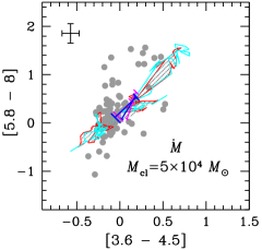
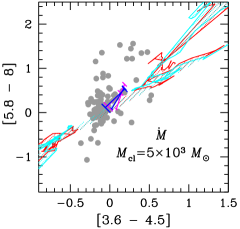
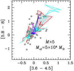
Figure 6: Comparison between models and Magellanic individual star clusters: [5.8 - 8] versus [3.6 - 4.5]. Gray filled circles are reddening-corrected clusters from the sample in Table 4, and black bars represent typical photometric errors. Colored regions illustrate model SSPs and expected $\pm 1\ \sigma$ error bars. Top left: fiducial $\dot{M}$ and 5$\times 10^{4}M_{\odot}$; top right: fiducial $\dot{M}$ and 5$\times 10^{3}M_{\odot}$; bottom left: $5\times$ fiducial $\dot{M}$ and 5$\times 10^{4}M_{\odot}$. Cyan: $Z=0.008$; red: $Z=0.017$. The models range in age between 3.5 Myr and 14 Gyr. Blue and magenta tick marks indicate 0.01, 0.3, 1, 5, 13 Gyr, respectively for $Z=0.008$ and $Z=0.017$; larger tick mark size represents increasing age.

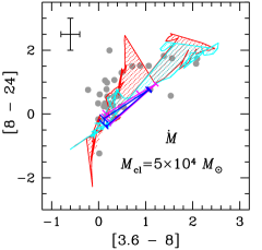
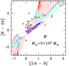
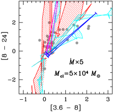
Figure 7: Comparison between models and Magellanic individual star clusters: [8 - 24] versus [3.6 - 8]. The symbols and models have the same meanings as in Fig. 6.

3.3 “Superclusters.”

I have also obtained the integrated fluxes and the SBF measurements of artificial “superclusters,” assembled by adding together all the clusters in one SWB (or pre-SWB) class, as I have done before (González et al., 2004; González-Lópezlira et al., 2005, 2010). This procedure reduces the stochastic effects due to small numbers of stars in short-lived evolutionary phases, in particular the TP-AGB. Before coaddition, the SMC clusters are geometrically magnified, conserving flux, to place them at the distance of the LMC, and all (dereddened and sky-subtracted) clusters in a class are scaled to a common photometric zero-point and registered to a common center. The integrated fluxes of the superclusters are derived in the same fashion as for individual clusters. Measured colors for all superclusters are presented in Table 5, together with their ages, metallicities, and photometric masses –derived from the comparison between 2MASS (Skrutskie et al., 1997) $J$, $H$, and $K_{s}$ supercluster mosaics and CB^∗ models.

Table 5: Integrated Colors and Fluctuation Magnitudes of Magellanic Superclusters

Supercluster	Log age (year)a	$Z$	Mass (10${}^{6}M_{\odot}$)b	[3.6 - 4.5]	[3.6 - 8]	[5.8 - 8]	[8 - 24]	$\mbox{$\bar{M}$}_{3.6}$	$\mbox{$\bar{M}$}_{4.5}$	$\mbox{$\bar{M}$}_{5.8}$	$\mbox{$\bar{M}$}_{8}$	$\mbox{$\bar{M}$}_{24}$
pre	6.78$\pm$0.62	0.010$\pm$0.005c	0.08 $\pm$ 0.02	0.19$\pm$0.29	2.50$\pm$0.52	1.23$\pm$0.23	3.56$\pm$0.36	-11.35$\pm$0.19	-11.20$\pm$0.15	-11.28$\pm$0.19	-13.37$\pm$0.36	-11.25$\pm$0.52
I	7.51$\pm$0.32	0.010$\pm$0.005c	0.6 $\pm$ 0.1	-0.04$\pm$0.14	0.62$\pm$0.15	0.21$\pm$0.15	0.07$\pm$0.39	-10.69$\pm$0.10	-10.60$\pm$0.12	-10.72$\pm$0.14	-11.5$\pm$0.17	$\cdots$
II	7.88$\pm$0.25	0.010$\pm$0.005c	0.5 $\pm$ 0.1	-0.17$\pm$0.11	-0.09 $\pm$0.15	-0.15$\pm$0.14	2.01$\pm$0.16	-8.96 $\pm$0.20	-9.00$\pm$0.21	-9.07$\pm$0.22	-9.75$\pm$0.23	-10.00$\pm$0.51
III	8.21$\pm$0.29	0.010$\pm$0.005d	0.4 $\pm$ 0.1	-0.14$\pm$0.08	1.00$\pm$0.10	0.61$\pm$0.07	2.23$\pm$0.21	-8.28$\pm$0.18	-8.20$\pm$0.14	-8.33$\pm$0.19	-8.96$\pm$0.38	-13.26$\pm$0.48
IV	8.65$\pm$0.36	(3$\pm$2)e-3d	0.4 $\pm$ 0.0	-0.10$\pm$0.20	0.18$\pm$0.30	0.05$\pm$0.29	-0.21$\pm$0.71	-9.30$\pm$0.20	-9.47$\pm$0.24	-9.64$\pm$0.29	-10.57$\pm$0.22	-12.02$\pm$0.40
V	9.09$\pm$0.29	(4$\pm$2)e-3d	1.4 $\pm$ 0.1	-0.17$\pm$0.13	0.45$\pm$0.45	0.26$\pm$0.32	-0.74$\pm$0.34	-8.69$\pm$0.12	-9.17$\pm$0.29	-10.20$\pm$0.43	-11.64$\pm$0.40	-9.32$\pm$0.46
VI	9.45$\pm$0.28	(2$\pm$1)e-3d	2.4 $\pm$ 0.1	-0.07$\pm$0.09	2.27$\pm$0.07	1.74$\pm$0.10	0.00$\pm$1.26	-8.49 $\pm$0.25	-8.73$\pm$0.40	-8.79$\pm$0.47	-8.83$\pm$0.46	$\cdots$
VII	9.82$\pm$0.29	(7$\pm$4)e-4d	2.4 $\pm$ 0.3	-0.08$\pm$0.08	0.23$\pm$0.07	0.07$\pm$0.07	0.31$\pm$0.11	-6.79 $\pm$0.36	-6.54$\pm$0.50	-7.00 $\pm$ 0.28	-7.88 $\pm$ 0.60	$\cdots$

^a From the calibration of the $S$-parameter by Girardi et al. (1995).

^b Masses from near-IR mass-to-light ratios (2MASS data and CB^∗ models); errors are equal to the dispersion of the results at $J$, $H$, and $K_{s}$.

^c Cohen (1982).

^d Frogel et al. (1990), assuming $Z_{\odot}=0.017$.

Figures 8 and 9 display the same two-color diagrams shown previously (respectively, [5.8 - 8] versus [3.6 - 4.5] and and [8 - 24] versus [3.6 - 8]), now comparing the models to the Magellanic artificial superclusters. In all the panels, the data (solid black circles with error bars) are plotted together with models of different metallicities ($Z$ = 0.0005, blue; 0.008, cyan; 0.017, red), that bracket those of the superclusters (0.0007 $\leq Z\leq$ 0.01; Frogel et al. 1990, assuming that $Z_{\odot}=0.017$; Cohen 1982). Three different theoretical mass-loss rates are shown: fiducial $\dot{M}$ (top left), fiducial $\dot{M}/5$, and 5$\times$ fiducial $\dot{M}$. The expected $\pm 1\sigma$ error bars for the models (colored bands) have been calculated assuming a stellar population of $5\times 10^{5}~{}M_{\odot}$. Models with a mass-loss rate higher than fiducial seem more consistent with the data, especially those of the pre-SWB and SWB VI superclusters. However, I note here that the pre-SWB supercluster may be subject to more stochastic fluctuations, given its lower mass, and may be more affected by additional extinction than older objects. Also, as I have argued before (González-Lópezlira et al., 2010), the assumption that the addition of many small objects is statistically equal to a large one will fail, if none of the small clusters are massive enough to produce the most massive stars (e.g., Weidner & Kroupa, 2006); this deficiency will be an issue during the first few 10⁷ yr, when such stars contribute most of the cluster’s light.

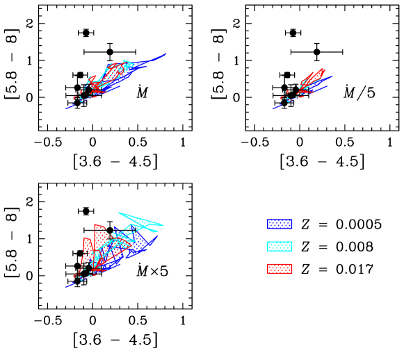
Figure 8: Comparison between models and MC “superclusters”: two-color diagram, [5.8 - 8] versus [3.6 - 4.5]. Top left: fiducial $\dot{M}$; top right: fiducial $\dot{M}$/5; bottom left: fiducial $\dot{M}\times 5$. Filled circles are artificial “superclusters” built in this work, following González et al. (2004). Colored regions represent SSPs with chosen mass-loss rate and expected $\pm 1\sigma$ error bars for 5$\times 10^{5}~{}M_{\odot}$. Blue: $Z=$ 0.0005; cyan: $Z=$ 0.008; red: $Z=$ 0.017. Supercluster ages go from $\sim$ 6 Myr to $\sim$ 7 Gyr; model ages span between 3 Myr and 14 Gyr.

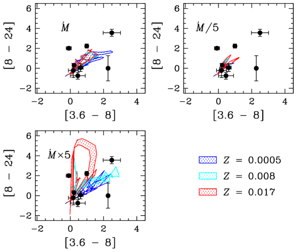
Figure 9: Comparison between models and MC “superclusters”: two-color diagram, [8 - 24] versus [3.6 - 8]. The symbols and models have the same meanings as in Fig. 8.

It is also useful to compare data and models in the age-color plane. I carry out this exercise in Figure 10, once again using models with different metallicities and mass-loss rates. The [3.6 - 4.5] color data (top row) show a nearly flat behavior with age, with the only possible exception being the pre-SWB cluster, which appears to have excess reddening. The flat behavior of superclusters from SWB II to VI –the age range sensitive to changes in $\dot{M}$– is best reproduced, for the low metallicities of the Magellanic clusters, by fiducial $\dot{M}/5$, although $\dot{M}$ cannot be excluded, given measurement errors and model uncertainties. Conversely, models with $\dot{M}$ and $5\times\dot{M}$ appear to almost equally well reproduce [3.6 - 8], [5.8 - 8], and [8 - 24] color data. In particular, at [3.6 - 8] and [5.8 - 8] (second and third rows), the SWB VI cluster is slightly more consistent with the lowest $Z$, 5 $\times\dot{M}$ models; the peak at 1–2 Gyr survives for models with $Z$ = 0.002, i.e., those closest to the metallicity of the SWB VI cluster. In conclusion, although models are compatible with the observations, integrated colors cannot strongly constrain the mass-loss rate, given the present data and theoretical uncertainties. In the next section, I will discuss the relationship between surface brightness fluctuations and mass-loss rates in global stellar populations.

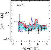
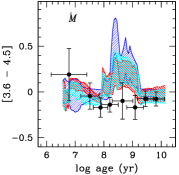
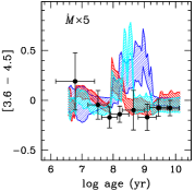
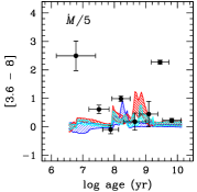
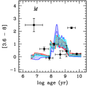
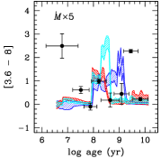
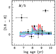
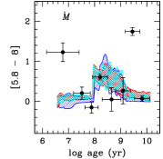
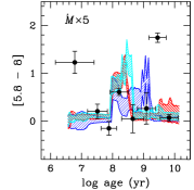
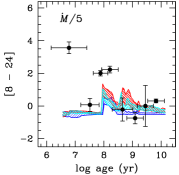
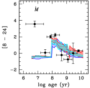
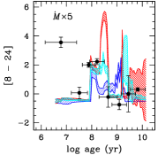
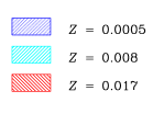
Figure 10: Comparison between models and MC “superclusters,” colors versus log (age). From top to bottom: [3.6 - 4.5], [3.6 - 8], [5.8 - 8], [8 - 24]. The symbols and models have the same meanings as in Fig. 8.

4 Surface Brightness Fluctuations.

The fluctuation magnitude ($\bar{m}$) is the ratio between the variance and the mean of the stellar luminosity function (Tonry & Schneider, 1988; Tonry et al., 1990), normalized by $(4\pi d^{2})$, where $d$ is the distance. This can be expressed by the following equation:

$$\mbox{$\bar{m}$}=-2.5\ {\rm log}\ \frac{1}{4\pi d^{2}}\frac{\Sigma n_{i}l_{i}^{2}}{\Sigma n_{i}l_{i}}+{\rm zeropoint},$$ (1)

where $n_{i}$ and $l_{i}$ are the number of stars of type $i$ and their luminosity, respectively.

Because of the dependency on the square of the stellar luminosity, the sum in the numerator is dominated by the brightest stars. Hence, $\bar{m}$ is especially sensitive to and informative about the most luminous stars in a given band and at a particular evolutionary phase of a population. TP-AGB stars in the mid-IR are clearly a case in point. In what follows, I will calculate the fluctuation magnitudes of the MC superclusters in the Spitzer IRAC bands and MIPS [24] filter.

The integrated fluxes of the superclusters, calculated as described in Section 3.3, were used for the denominator of eq. 1 –the sum of $n_{i}l_{i}$ converges slowly, and low-mass stars fainter than the detection limit cannot be added individually. The sum in the numerator, on the other hand, converges quickly, and was found by summing the flux, squared, of resolved bright stars in the SAGE Winter ’08 IRAC Epoch 1 and Epoch 2 Archive, and the SAGE Winter ’08 MIPS 24 $\mu$m Epoch 1 and Epoch 2 Catalog (IPAC 2009). Before adding the squared fluxes in the numerator, though, the field stars were statistically removed following the procedure presented in Mighell et al. (1996), and described also in González-Lópezlira et al. (2010) for 2MASS near-IR data. Basically, the [3.6 - 8] versus [8] CMD of the stars within 1$\arcmin$ of the supercluster center (the “cluster region,” which presumably includes both cluster and field stars) is compared to the CMD of the stars in the annulus with 2$\farcm$0 $<r\leq$ 2$\farcm$5 (i.e., the “field”). For each star in the cluster region with mag [8] $\pm\sigma_{[8]}$ and color [3.6 - 8] $\pm\sigma_{[3.6-8]}$, I count the number of stars in the same CMD with [3.6 - 8] colors within $\pm$MAX(2$\sigma_{[3.6-8]}$,0.100) mag and [8] mag within $\pm$MAX(2$\sigma_{[8]}$,0.200) mag. I call this number $N_{\rm scl}$. I also count the number of stars in the field CMD within the same $\Delta$ [8] by $\Delta$ [3.6 - 8] bin determined from the cluster star. This is $N_{\rm fld}$. The probability $p$ that the star in the cluster region CMD actually belongs to the supercluster can be expressed as

$$p\approx 1-{\rm MIN}\left(\frac{\alpha(N_{\rm fld}+1)}{N_{\rm scl}+1},1.0\right),$$ (2)

where $\alpha$, in this case 0.44, is the ratio of the area of the cluster region ($\pi$ arcmin²) to the area of the field region (2.25 $\pi$ arcmin²). Once $p$ is calculated for a given star, it is compared to a randomly drawn number $0\leq p^{\prime}\leq 1$. If $p\geq p^{\prime}$, the star is accepted as a supercluster member; otherwise, it is considered as a field object and rejected.

Figures 11 and 12 display the [3.6 - 8] versus [8] CMDs for our 8 “superclusters.” The decontaminated cluster sources are represented with black solid dots, while the contaminating field stars are shown with gray dots. Theoretical isochrones from CB^∗ models have been overplotted on the decontaminated sources as solid brown lines. The mean ages and metallicities of the model isochrones are approximately the same as those reported in Table 5, except for the pre-SWB supercluster, for which the isochrone is a few Myr older (10 Myr versus 6 Myr). For comparison, analogous [$J-K_{s}$] versus $K_{s}$ CMDs, from 2MASS data, are shown to the right of each mid-IR graph. Photometric errors as a function of magnitude for individual stars are shown in Figure 13; from top to bottom: $\Delta$ [3.6], $\Delta$ [8], $\Delta\ J$, and $\Delta\ K_{s}$.

There are not enough 24 $\mu$m sources to perform a meaningful decontamination of the MIPS data following the above procedure. Instead, I determine the cluster star list in this band by matching the sources in the “cluster region” with the decontaminated IRAC sample.

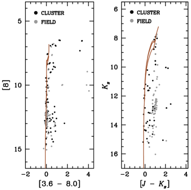
(a) Pre-SWB. Isochrone $Z=$ 0.008; age = 10 Myr.

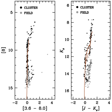
(b) SWB I. Isochrone $Z=$ 0.008; age = 32 Myr.

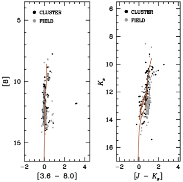
(c) SWB II. Isochrone $Z=$ 0.008; age = 76 Myr.

(d) SWB III. Isochrone $Z=$ 0.008; age = 160 Myr.

Figure 11: Color-magnitude diagrams of MC superclusters, SWB classes pre-SWB (top left), I (top right), II (bottom left), and III (bottom right). Left panels: apparent 8 $\mu$m mag, [8], vs. [3.6 - 8] color; right panels: apparent $K_{s}$-band mag vs. [$J$ - $K_{s}$] color. Solid black dots: Supercluster decontaminated stars within 60$\arcsec$ from the center (at the distance of the LMC); solid gray dots: contaminating field stars (see the text). Solid brown lines: theoretical isochrones from CB^∗ models, with indicated ages and metallicities. These are approximately the same as those estimated for the superclusters (Table 4), except for the pre-SWB supercluster, for which the isochrone is a few Myr older (10 Myr versus 6 Myr; see the text).

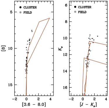
(a) SWB IV. Isochrone $Z=$ 0.004; age = 450 Myr.

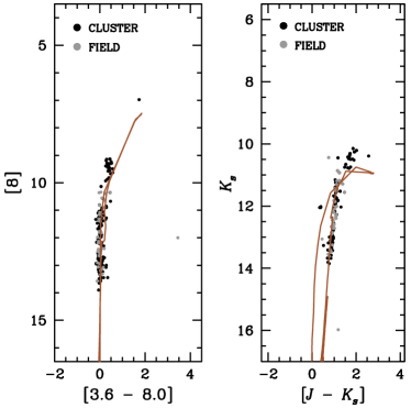
(b) SWB V. Isochrone $Z=$ 0.004; age = 1.2 Gyr.

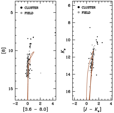
(c) SWB VI. Isochrone $Z=$ 0.002; age = 2.8 Gyr.

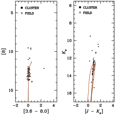
(d) SWB VII. Isochrone $Z=$ 0.001; age = 6.5 Gyr.

Figure 12: Color-magnitude diagrams of MC superclusters, SWB classes IV (top left), V (top right), VI (bottom left), and VII (bottom right). The models and symbols have the same meanings as in Figure 11.

Figure 13: Photometric errors as a function of magnitude for individual stars. Top row: $\Delta$ [3.6]; second row: $\Delta$ [8]; third row: $\Delta\ J$; bottom row: $\Delta\ K_{s}$.

I have used the models to check that the stars that have been detected as point sources in the SAGE mosaics are enough to obtain a reliable estimate of the mid-IR SBFs of the Magellanic star clusters. In this experiment, SBF magnitudes are calculated from models as done for observations, that is, the denominator of eq. 1 is always the sum of all the stars in the isochrone, while the stars considered in the numerator are only those brighter than the data detection limit. Figure 14 shows, for $Z=$ 0.0005, 0.004, 0.008, 0.017, and 0.04, the difference between the 3.6, 4.5, 5.8, and 8 $\mu$m integrated and fluctuation magnitudes calculated with all the stars, and only from those with $M_{5.8}\leq-4.5$ (or [5.8] = 14 mag at the LMC, and 14.5 mag at the SMC). This difference is in fact an overestimate, since fainter stars are detected. Barring ages younger than $\sim$ 2 Myr, which are hardly relevant to the clusters in this work, at all times the anticipated differences in the derived fluctuation magnitudes for all IRAC bands are smaller than the expected errors, due mainly to stochastic fluctuations in the number of stars (see Table 5); in fact, for ages younger than a few Gyr, the differences are barely noticeable. This is true even for the oldest clusters, in which the contribution from bright stars to the integrated luminosity is of the order of 30% – 50%, depending on metallicity.

Figure 14: Comparison between contributions to integrated and fluctuation magnitudes from all stars in the isochrone ($\Delta$ mag = 0), and only from stars brighter than $M_{5.8}$ = -4.5 (or [5.8] = 14.0 mag at the LMC, and 14.5 mag at the SMC). Top left panel: $Z$ = 0.0005; top right panel: $Z$ = 0.004; middle left panel: $Z$ = 0.008; middle right panel: $Z$ = 0.017; bottom left panel: $Z$ = 0.04. Displayed Within each panel is the difference in integrated magnitudes at [3.6] (short–dashed line), [4.5] (long–dashed line), [5.8] (dotted line), [8] (dotted–long–dashed line), and for fluctuation magnitudes in all the IRAC bands (thick solid line).

Figure 15 displays a similar plot for the MIPS 24 $\mu$m band, including only stars with $M_{24}\leq-9.0$ (or [24] = 9.5 and 10.0 mag at the LMC and SMC, respectively). This graph shows that there are not enough stars to calculate SBFs for populations with ages between $\sim$ 15 and 100 Myr, regardless of metallicity. Also, SBFs cannot be accurately derived after 1.5 Gyr for $Z$ between 0.0005 and 0.004, and after 4 Gyr for $Z$ = 0.008.

Figure 15: Comparison between contributions to 24 $\mu$m integrated and fluctuation magnitudes from all stars in the isochrone ($\Delta$ mag = 0), and only from stars brighter than $M_{24}$ = -9. (or [24] = 9.5 mag at the LMC, and 10.0 mag at the SMC). Dashed line: difference in integrated magnitudes; solid line: difference in fluctuation magnitudes. Metallicities are the same as in Figure 14.

The SBF magnitudes of the Magellanic superclusters in the IRAC bands and at [24] are presented in Table 5. Unreliable values, per Figure 15, are obviously omitted.

For comparison with the data, I compute the time evolution of SBF magnitudes of single-burst stellar populations in the IRAC and 24 $\mu$m bands, with the metallicities and helium contents available in the CB^∗ models. Figure 16 shows absolute fluctuation magnitudes versus log (age) for CB^∗ models with fiducial mass-loss rate and different metallicities, from $Z$ = 0.0005 ($\sim$ 1/34 solar) to $Z=$ 0.04 ($\sim$ 2.4 times solar). Colored regions delimit expected $\pm$ 1 $\sigma$ stochastic errors for a stellar population with $5\times 10^{5}~{}M_{\odot}$. At very young ages (around 10 Myr), the red supergiants produced by the models with the lowest $Z=0.0005$ are fewer and fainter in the mid-IR; hence the SBF magnitudes of these populations are also fainter, and suffer from a larger stochastic error. In contrast, at intermediate ages ($\sim$ 200 Myr to 1 Gyr), when TP-AGB stars are predominant, the SBF magnitudes of the population with $Z=0.04$ are faintest between [4.5] and [8]: its TP-AGB stars are also faintest; here, opacity is seemingly more important than temperature.

Finally, after 1 Gyr, when cluster luminosities are dominated by red giant branch (RGB) stars, the opposite is true, and we get the more intuitive result that there is a strong trend with metallicity and wavelength: mid-IR SBF magnitudes will be brighter for higher metallicities, and the difference in SBF brightness between the lowest and highest $Z$ will increase with $\lambda$.

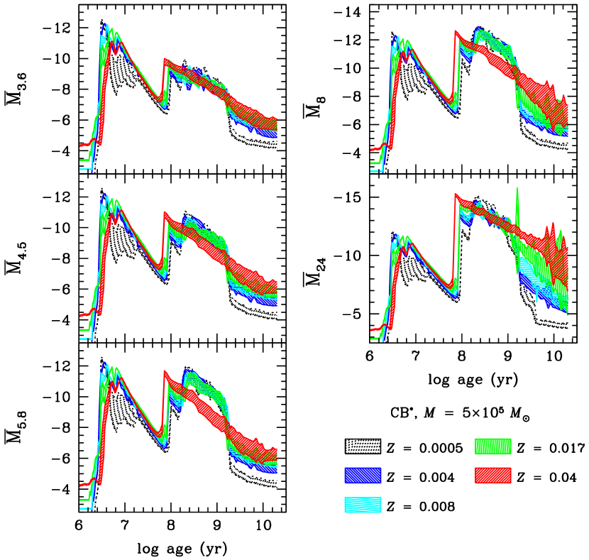
Figure 16: Absolute fluctuation magnitudes versus log (age) for standard CB^∗ models with different metallicities. Colored regions delimit expected $\pm 1\sigma$ stochastic errors for stellar populations with $5\times 10^{5}~{}M_{\odot}$. Black dotted: $Z$ = 0.0005; blue left-hatched: $Z$ = 0.004; cyan horizontal-hatched: $Z$ = 0.008; green vertical-hatched: $Z$ = 0.017; red right-hatched: $Z$ = 0.04.

I now compare the models to our MC supercluster data. Figure 17 presents mid-IR (3.6 to 24 $\mu$m) absolute SBF magnitudes versus log (age) for MC clusters younger than $\sim$ 160 Myr, plotted together with models with $Z=0.008$, and 3 different mass-loss rates: fiducial $\dot{M}$ (cyan), fiducial $\dot{M}/5$ (blue), and fiducial $\dot{M}\times 5$ (red); again, colored regions delimit expected $\pm 1\sigma$ stochastic errors for a stellar population with $5\times 10^{5}M_{\odot}$. Before the onset of the TP-AGB phase at $\sim$ 100 Myr, models are degenerate, but both models and data show the same trend of diminishing SBF strength with time. (Supercluster type SWB I is omitted at 24 $\mu$, on account of insufficient statistics to obtain its SBF magnitude in this filter.)

I note that SBF magnitudes at 4.5, 5.8, and 8 $\mu$m can clearly discern between global changes in the mass-loss rates for intermediate-age populations, in particular between $\sim 10^{8}$ yr –the onset of the TP-AGB phase– and 1 Gyr. During most of this time span, the SBF magnitudes of a population with fiducial $\dot{M}$ will be brighter than those for stars with a reduced mass-loss rate. A population with 5$\times\dot{M}$, on the other hand, will harbor more bright stars at the beginning and hence display SBF magnitudes with a smaller dispersion. However, TP-AGB lifetimes will be reduced according to the fuel-consumption theorem (Renzini & Buzzoni, 1986), and this will cause the SBF values, first to oscillate, and after age $\sim$ 400 Myr to remain lower than those for the population with $\dot{M}/5$. Then, between 2 and 5 Gyr –once the RGB dominates–, and from 3.6 to 5.8 $\mu$m, the dispersion will grow, due to the appearance of a few bright red giant stars; only at 8 and 24 $\mu$m is there also an increase of the SBF brightness at these times.

In Figure 18, data of superclusters types SWB IV and V are compared to models with $Z=0.004$. The fit is quite good, and overall consistent with the fiducial mass-loss rate. Finally, Figures 19 and 20 show cluster types SWB VI and VII together with, respectively, models with $Z=0.002$ and $Z=0.001$, from 3.6 to 8 $\mu$m (as the data have insufficient statistics at 24 $\mu$m). At the age of cluster type VI the TP-AGB phase shuts off, hence the SBF magnitudes change abruptly and sensitivity to $\dot{M}$ is poor. The fit between models and data points, however, is fair within the errors. On the other hand, the derived SBF magnitudes of cluster type VII are too bright at all wavelengths, compared to the model. This problem could be explained if the handful of stars brighter than [8] = 11.5 mag (see Figure 12, bottom right panel) are actually foreground in the Milky Way halo, for example, and thus our decontamination scheme did not work properly.

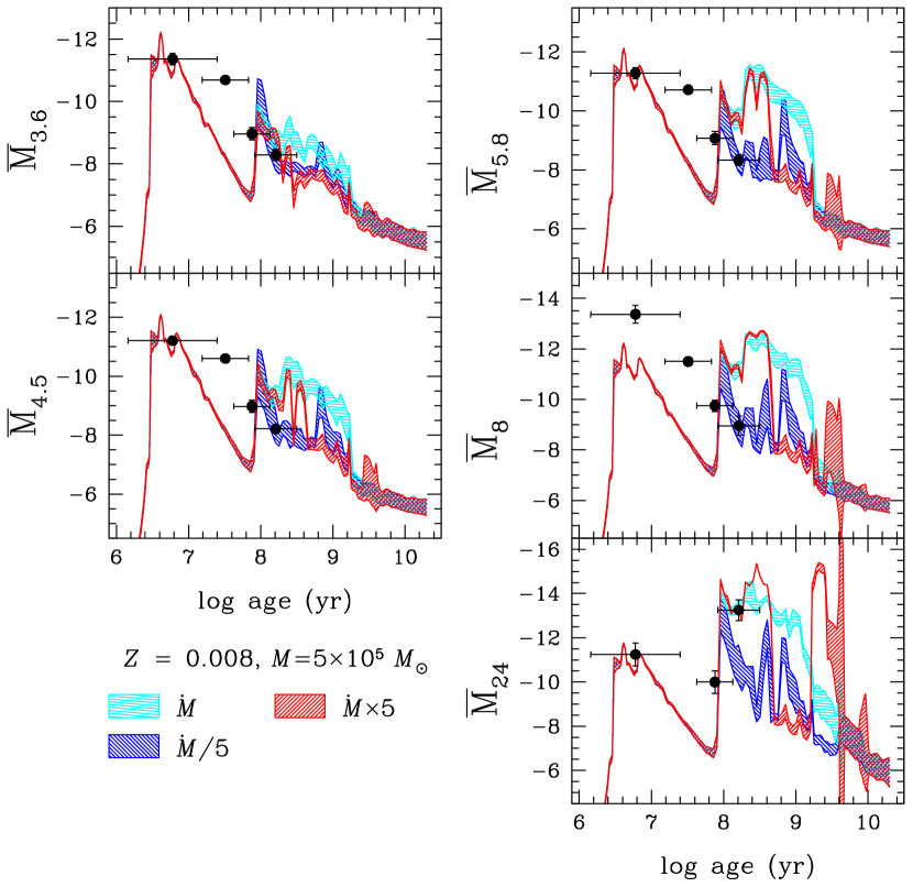
Figure 17: SBFs of Magellanic star clusters I. Observations of young and intermediate-age MC superclusters (pre-SWB to SWB III) are compared to models with $Z$ = 0.008. $\pm 1\sigma$ stochastic uncertainties are shown for stellar populations with 5 $\times 10^{5}~{}M_{\odot}$. Cyan horizontal-hatched: fiducial $\dot{M}$; blue left-hatched: fiducial $\dot{M}$/5; red right-hatched: fiducial $\dot{M}\times$5. Solid circles: mid-IR SBF measurements. Statistics are insufficient to obtain an SBF magnitude at 24 $\mu$m for the supercluster type SWB I.

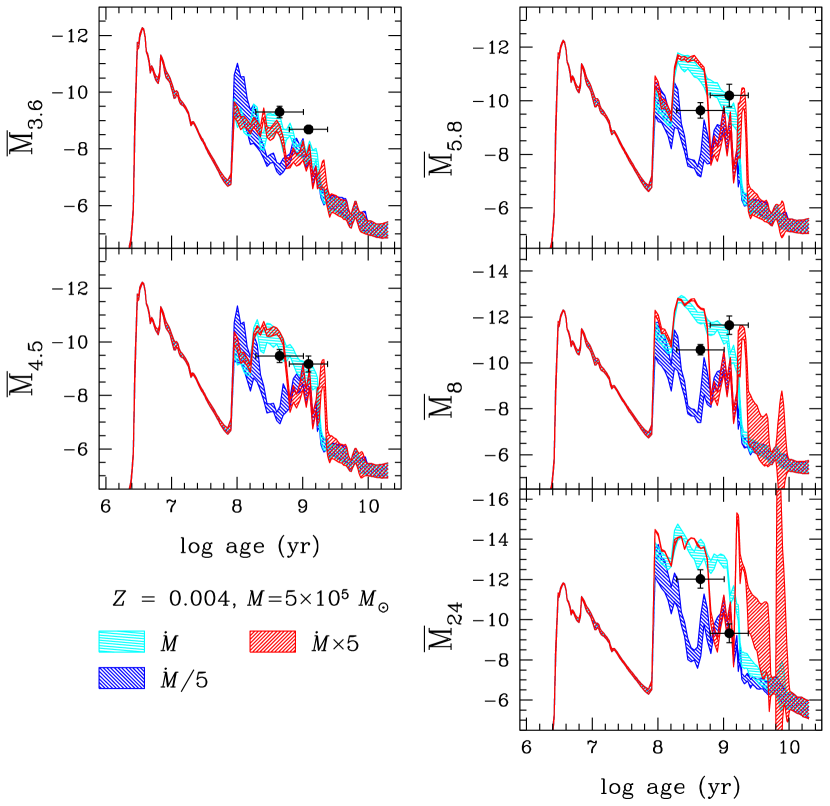
Figure 18: SBFs of Magellanic star clusters II. Observations of intermediate-age MC superclusters (SWB IV and SWB V) are compared to models with $Z$ = 0.004. $\pm 1\sigma$ stochastic uncertainties are shown for stellar populations with $5\times 10^{5}~{}M_{\odot}$, coded as in Figure 17.

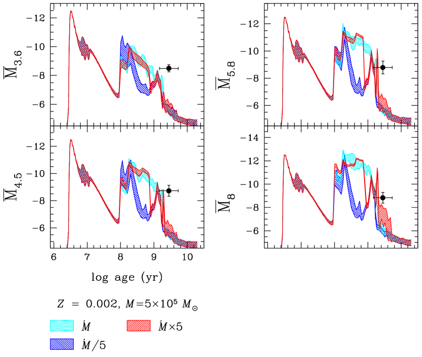
Figure 19: SBFs of Magellanic star clusters III. Observations of the old MC supercluster SWB VI are compared to models with $Z$ = 0.002. $\pm 1\sigma$ stochastic uncertainties are shown for stellar populations with $5\times 10^{5}~{}M_{\odot}$, coded as in Figure 17.

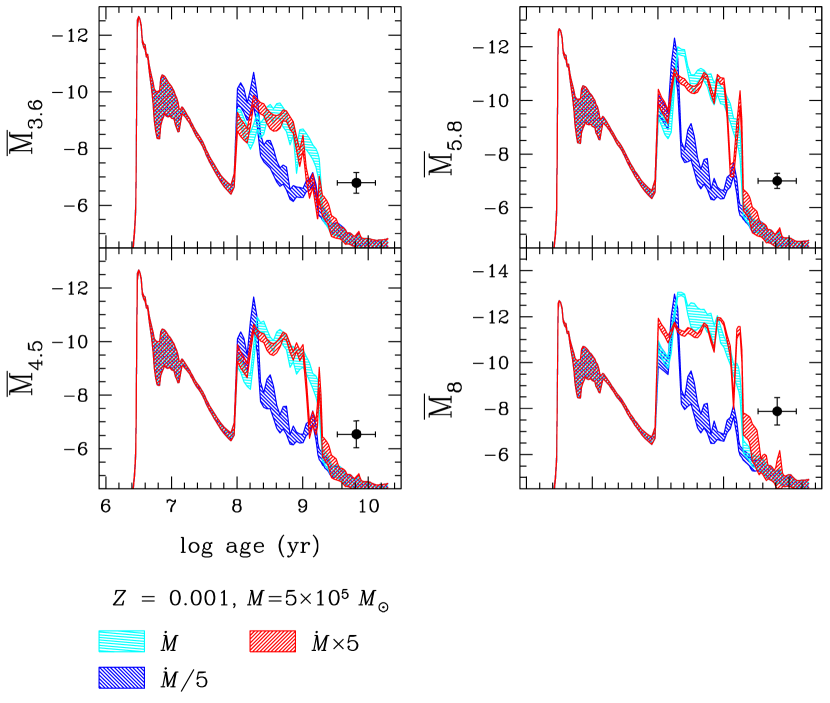
Figure 20: SBFs of Magellanic star clusters IV. Observations of the old MC supercluster SWB VII are compared to models with $Z$ = 0.001. $\pm 1\sigma$ stochastic uncertainties are shown for stellar populations with $5\times 10^{5}~{}M_{\odot}$, coded as in Figure 17.

5 Summary and Conclusions.

I have presented mid-IR broadband colors and fluctuation magnitudes computed from SSP models, with the main goal of exploring their ability to detect changes in the global mass-loss rate of stars undergoing the TP-AGB phase. To this end, I have used the CB^∗ evolutionary tracks to produce spectra of TP-AGB stars, considering the radiative transfer in their circumstellar envelopes. I have processed SEDs for fiducial $\dot{M}$, as well as for twice, 5$\times$, 10$\times$ fiducial, $\dot{M}/2$, $\dot{M}/5$, and $\dot{M}/10$. In all cases, the stellar parameters, mass-loss rate, and length of the superwind evolutionary phase have been varied simultaneously and consistently, as described in González-Lópezlira et al. (2010). The model colors and SBF magnitudes have then been compared to mid-IR data of single AGB stars and star clusters in the Magellanic Clouds. My conclusions are as follows:

• Models with different mass-loss rates and metallicities differ significantly in their predicted mid-IR colors and SBF magnitudes.

• Models with a higher than fiducial mass-loss rate are needed to fit the mid-IR colors of “extreme” single AGB stars in the LMC.

• The range of mid-IR colors of individual MC clusters is consistent with models with $Z=0.008$, a mass-loss rate between fiducial and 5 $\times$ fiducial, and the stochastic errors expected for a cluster population between 5 $\times 10^{3}$ and 5 $\times 10^{4}M_{\odot}$.

• In the case of artificial “superclusters,” built by grouping clusters in the MCs by age and metallicity, although models are compatible with the observations, integrated colors cannot strongly constrain the mass-loss rate, given the present data and theoretical uncertainties. The colors of the SWB VI cluster (3 Gyr), however, suggest a higher than fiducial mass-loss rate.

• Model SBF magnitudes are quite sensitive to metallicity for 4.5 $\mu$m and longer wavelengths, basically at all stellar population ages. For metallicities between $Z=0.004$ and $Z=0.04$ and populations younger than 1-2 Gyr, fluctuations grow fainter as $Z$ increases; for older populations the trend reverses, and SBFs are brighter for higher $Z$. For $Z=0.0005$, fluctuations are faintest for ages $<$ 100 Myr and $>$ 1-2 Gyr; in between, SBF magnitudes are as bright as for 0.004 $\lesssim Z\lesssim$ 0.017.

• Fluctuation magnitudes are powerful diagnostics of mass-loss rate in the TP-AGB.

• The SBF measurements of the MC superclusters suggest a mass-loss rate close to fiducial. Although consistent with the models within the errors, it is possible that the oldest SWB VII cluster (7 Gyr, and hence with the faintest RGB stars) is contaminated by foreground stars.

The present work has in fact performed an independent calibration of the CB^∗ models, and confirmed that colors and SBF magnitudes in the mid-IR are sensitive to global changes in mass-loss rate, in particular during the TP-AGB phase. For this kind of proof of concept work, the MC clusters offer the advantages of their known distances and wide range of metallicities. However, star clusters with masses lower than $\sim 5\times 10^{5}M_{\odot}$ may be subject to stochastic fluctuations in their population properties that can be significant. Colors and fluctuation magnitudes of whole galaxies obtained with the upcoming James Webb Space Telescope should be much less affected by these systematics, and hence able to measure with a high degree of confidence global mass-loss rates and their correlation (or not) with metallicity.

References

- Aringer et al. (2009) Aringer, B., Girardi, L., Nowotny, W., Marigo, P., & Lederer, M.T. 2009, A&A, 503, 913
- Bertelli et al. (2008) Bertelli, G., Girardi, L., Marigo, P., & Nasi, E. 2008, A&A, 484, 815
- Bowen & Willson (1991) Bowen, G. H., & Willson, L. A. 1991, ApJ, 375, L53
- Bruzual (2002) Bruzual A., G. 2002, in Extragalactic Star Clusters, IAU Symposium Ser., Vol. 207, eds. D. Geisler, E. K. Grebel, & D. Minniti, Provo:ASP, 616
- Bruzual (2010) Bruzual, G. 2010, Philosophical Transactions of the Royal Society of London Series A, 368, 783
- Bruzual & Charlot (2003) Bruzual, G., & Charlot, S. 2003, MNRAS, 344, 1000
- Bruzual et al. (2013) Bruzual, G., Charlot, S., González-Lópezlira, R.A., et al. 2013, in The Intriguing Life of Massive Galaxies, IAU Symposium Ser., Vol. 295, eds. D. Thomas, A. Pasquali, and I. Ferreras, Cambridge: Cambridge University Press, 282
- Cantiello et al. (2003) Cantiello, M., Raimondo, G., Brocato, E., & Capaccioli, M. 2003, AJ, 125, 2783
- Cerviño et al. (2002) Cerviño, Valls–Gabaud, Luridiana, & Mas–Hesse, J. M. 2002, A&A, 381, 51
- Chabrier (2003) Chabrier, G. 2003, PASP, 115, 763
- Cohen (1982) Cohen, J. G. 1982, ApJ, 258, 143
- Falcón-Barroso et al. (2011) Falcón-Barroso, J., Sánchez-Blázquez, P., Vazdekis, A., et al. 2011, A&A, 532, A95
- Ferrarese et al. (2000) Ferrarese, L., Ford, H. C., Huchra, J., et al. 2000, ApJS, 128, 431
- Frogel et al. (1990) Frogel, J.A., Mould, J., & Blanco, V.M., 1990, ApJ, 352, 96
- Girardi et al. (1995) Girardi, L., Chiosi, C., Bertelli, G., & Bressan, A. 1995, A&A, 298, 87
- Girardi et al. (2010) Girardi, L., Williams, B.F., Gilbert, K.M., Rosenfield, P., Dalcanton, J.J., Marigo, P., Boyer, M.L., Dolphin, A., Weisz, D.R., Melbourne, J., Olsen, K.A.G., Seth, A.C., & Skillman, E. 2010, ApJ, 724, 1030
- González et al. (2004) González, R. A., Liu, M. C., & Bruzual A., G. 2004, ApJ, 611, 270
- González-Lópezlira et al. (2005) González-Lópezlira, R. A., Albarrán, M. Y., Mouhcine, M., et al. 2005, MNRAS, 363, 1279
- González-Lópezlira et al. (2010) González-Lópezlira, R. A., Bruzual-A., G., Charlot, S., Ballesteros-Paredes, J., & Loinard, L. 2010, MNRAS, 403, 1213
- Gordon et al. (2011) Gordon, K. D., Meixner, M., Meade, M. R., et al. 2011, AJ, 142, 102
- Harris & Zaritsky (2004) Harris, J. & Zaritsky, D. 2004, AJ, 127,153
- Harris & Zaritsky (2009) Harris, J. & Zaritsky, D. 2009, AJ, 138,1243
- Iben (1984) Iben, I., Jr. 1984, ApJ, 277, 333
- Ivezić, Nenkova, & Elitzur (1999) Ivezić, Z., Nenkova, M., & Elitzur, M. 1999, User Manual for DUSTY, University of Kentucky Internal Report (http://www.pa.uky.edu/ moshe/dusty)
- Kriek et al. (2010) Kriek, M., Labbé, I., Conroy, C., Whitaker, K.E., van Dokkum, P.G., Brammer, G.B., Franx, M., Illingworth, G.D., Marchesini, D., Muzzin, A., Quadri, R.F., & Rudnick, G. 2010, ApJ, 722, L64
- La Barbera et al. (2012) La Barbera, F., Ferreras, I., de Carvalho, R. R., Bruzual, G., Charlot, S., Pasquali, A., & Merlin, E. 2012, MNRAS, 426, 2300
- Lançon & Mouhcine (2002) Lançon, A. & Mouhcine, M. 2002, A&A, 393, 167
- Lanz & Hubeny (2003a) Lanz, T., & Hubeny, I. 2003, ApJS, 146, 417
- Lanz & Hubeny (2003b) .2003, ApJS, 147, 225
- Lanz & Hubeny (2007) .2007, ApJS, 169, 83
- Le Borgne et al. (2003) Le Borgne, J.-F., Bruzual, G., Pelló, R., Lançon, A., Rocca-Volmerange, B., Sanahuja, B., Schaerer, D., Soubiran, C., & Vílchez-Gómez, R. 2003, A&A, 402, 433
- Lee et al. (2010) Lee, H.-c., Worthey, G., & Blakeslee, J. P. 2010, ApJ, 710, 421
- Maraston (1998) Maraston, C. 1998, MNRAS, 300, 872
- Maraston (2005) .2005, MNRAS, 362, 799
- Marigo & Girardi (2007) Marigo, P., & Girardi, L. 2007, A&A, 469, 239
- Marigo et al. (2013) Marigo, P., Bressan, A., Nanni, A., Girardi, L., & Pumo, M. L. 2013, MNRAS, 434, 488
- Marigo et al. (2008) Marigo, P., Girardi, L., Bressan, A., Groenewegen, M. A. T., Silva, L., & Granato, G. L. 2008, A&A, 482, 883
- Martins et al. (2005) Martins, L. P., González Delgado, R. M., Leitherer, C., Cerviño, M., & Hauschildt, P. 2005, MNRAS, 358, 49
- Meixner (2008) Meixner, M. 2008, PASA, 25, 149
- Meixner et al. (2006) Meixner, M., Gordon, K. D., Indebetouw, R., et al. 2006, AJ, 132, 2268
- Melbourne et al. (2012) Melbourne, J., Williams, B.F., Dalcanton, J.J., Rosenfield, P., Girardi, L., Marigo, P., Weisz, D., Dolphin, A., Boyer, M.L., Olsen, K., Skillman, E., & Seth, A.C. 2012, ApJ, 748, 47
- Mighell et al. (1996) Mighell, K. J., Rich, R. M., Shara, M., & Fall, S. M. 1996, AJ, 111, 2314
- Nenkova et al. (2000) Nenkova, M., Ivezić, Ž., & Elitzur, M. 2000, in Thermal Emission Spectroscopy and Analysis of Dust, Disks, and Regoliths, ASP Conference Ser., Vol. 196, eds. M. L. Sitko, A. L. Sprague, and D. K. Lynch, San Francisco: Astronomical Society of the Pacific, 77
- Persson et al. (1983) Persson, S. E., Aaronson, M., Cohen, J. G., Frogel, J. A., & Matthews, K. 1983, ApJ, 266, 105
- Piovan et al. (2003) Piovan, L., Tantalo, R., & Chiosi, C. 2003, A&A, 408, 559
- Prugniel et al. (2011) Prugniel, P., Vauglin, I., & Koleva, M. 2011, A&A, 531, A165
- Raimondo et al. (2005) Raimondo, G., Brocato, E., Cantiello, M., & Capaccioli, M. 2005, AJ, 130, 2625
- Raimondo (2009) Raimondo, G. 2009, ApJ, 700, 1247
- Rauch (2003) Rauch, T. 2003, A&A, 403, 709
- Rayner et al. (2009) Rayner J.T., Cushing, M.C., & Vacca, W.D. 2009, ApJS, 185, 289
- Reimers (1975) Reimers, D. 1975, Memoires of the Societe Royale des Sciences de Liege, 8, 369
- Reimers (1977) .1977, A&A, 61, 217
- Renzini & Buzzoni (1986) Renzini, A., & Buzzoni, A. 1986, in Spectral Evolution of Galaxies, Astrophysics and Space Science Library, Vol. 122, eds. C. Chiosi, A. Renzini, Dordrecht:Springer, 195
- Rodríguez-Merino et al. (2005) Rodríguez-Merino, L. H., Chavez, M., Bertone, E., & Buzzoni, A. 2005, ApJ, 626, 411
- Rosenfield et al. (2014) Rosenfield, P., Marigo, P., Girardi, L., et al. 2014, ApJ, 790, 22
- Rosenfield et al. (2016) .2016, ApJ, 822, 73
- Sánchez-Blázquez et al. (2006) Sánchez-Blázquez, P., Peletier, R.F., Jiménez-Vicente, J., Cardiel, N., Cenarro, A.J., Falcón-Barroso, J., Gorgas, J., Selam, S., & Vazdekis, A. 2006, MNRAS, 371, 703
- Schlegel et al. (1998) Schlegel, D. J., Finkbeiner, D. P., & Davis, M. 1998, ApJ, 500, 525
- Searle et al. (1980) Searle, L., Wilkinson, A., & Bagnuolo, W. G. 1980, ApJ, 239, 803
- Skrutskie et al. (1997) Skrutskie, M. F., Schneider, S. E., Stiening, R., et al. 1997, in The Impact of Large Scale Near–IR Sky Surveys, Astrophysics and Space Science Library, Vol. 210, eds. F. Garzón, N. Epchtein, A. Omont, B. Burton, P. Persi, Dordrecht: Springer, 25
- Srinivasan et al. (2009) Srinivasan, S., Meixner, M., Leitherer, C., et al. 2009, AJ, 137, 4810
- Suh (2002) Suh, K.-W. 2002, MNRAS, 332, 513
- Suh (2000) .2000, MNRAS, 315, 740
- Suh (1999) .1999, MNRAS, 304, 389
- Tonry et al. (1990) Tonry, J. L., Ajhar, E. A., & Luppino, G. A. 1990, AJ, 100, 1416
- Tonry & Schneider (1988) Tonry, J. & Schneider, D. P. 1988, AJ, 96, 807
- Weidner & Kroupa (2006) Weidner, C., & Kroupa, P. 2006, MNRAS, 365, 1333
- Westera et al. (2002) Westera, P., Lejeune, T., Buser, R., Cuisinier, F., & Bruzual, G. 2002, A&A, 381, 524
- Willson (2000) Willson, L. A. 2000, ARA&A, 38, 573
- Zibetti et al. (2012) Zibetti, S., Gallazzi, A., Charlot, S., Pierini, D., & Pasquali, A. 2013, MNRAS, 428, 1479