Stable equatorial ice belts at high obliquity in a coupled atmosphere-ocean model

Abstract

Various climate states at high obliquity are realized for a range of stellar irradiance using a dynamical atmosphere-ocean-sea ice climate model in an aquaplanet configuration. Three stable climate states are obtained that differ in the extent of the sea ice cover. For low values of irradiance the model simulates a Cryoplanet which has a perennial global sea ice cover. By increasing stellar irradiance, transitions occur to an Uncapped Cryoplanet with a perennial equatorial sea ice belt, and eventually to an Aquaplanet with no ice. Using an emulator model we find that the Uncapped Cryoplanet is a robust stable state for a range of irradiance and high obliquities and contrast earlier results that high-obliquity climate states with an equatorial ice belt may be unsustainable or unachievable. When the meridional ocean heat flux is strengthened, the parameter range permitting a stable Uncapped Cryoplanet decreases due to melting of equatorial sea ice. Beyond a critical threshold of meridional ocean heat flux, the perennial equatorial ice belt disappears. Therefore, a vigorous ocean circulation may render it unstable. Our results suggest that perennial equatorial ice cover is a viable climate state of a high-obliquity exoplanet. However, due to multiple equilibria, this state is only reached from more glaciated, but not from less glaciated conditions.

1 Introduction

Orbital configurations such as obliquity and stellar irradiance are key determinants of the surface temperature of a planet (e.g., Pierrehumbert, 2010; Ferreira et al., 2014; Kaspi & Showman, 2015; Kilic et al., 2017a). Different combinations of these variables lead to a variety of states, such as a completely ice covered Cryoplanet, an ice free Aquaplanet, or combinations of these (Ferreira et al., 2014; Kilic et al., 2017a; Rose et al., 2017). Ferreira et al. (2014) explored the role of the ocean in controlling the surface temperature under high obliquity and suggested that the climate state with a perennial equatorial ice cover (Uncapped Cryoplanet) is unlikely to be stable due to the meridional structure of the ocean heat flux. Likewise, Rose et al. (2017) concluded based on an analytical latitude-energy balance model that a state with an equatorial ice belt may be stable but could not be reached in the presence of other equilibria such as ice-free and snowball states. On the other hand, Kilic et al. (2017a) using an atmospheric general circulation model (AGCM) coupled to a slab ocean found a stable uncapped cryoplanet state. This state was found stable for obliquities above 54° and a range of stellar irradiances. They pointed to the importance of initial conditions: in their simulations an Uncapped Cryoplanet was obtained only when the model was initialized in a cryoplanet state before increasing stellar irradiance. In the entire parameter region of the Uncapped Cryoplanet, there also exists the Aquaplanet as a second stable state. This implies that the state with an equatorial ice belt could not be reached from an aquaplanet initial state. This dependence on initial conditions is a characteristic of hysteresis behavior and the consequence of the broad occurrence of multiple equilibria in the obliquity-irradiance parameter space as shown by Kilic et al. (2017a). However, the precise shape of the hysteresis is strongly model and parameter dependent.

In this study we explore climate states at high obliquity using an AGCM coupled to a fully dynamical ocean model. In particular, we assess the role of the ocean heat transport for the uncapped cryoplanet state. The analysis focuses on the meridional energy flux of the atmosphere and the ocean which together determine the ice-free poles and the ice covered equatorial band. The results obtained by the dynamical atmosphere-ocean-sea ice model are complemented by a large number of simulations with an emulator model that consists of a dynamical atmosphere coupled to a slab ocean. The emulator, on which the earlier study of Kilic et al. (2017a) was based, permits us here to specifically explore the stability of the Uncapped Cryoplanet at obliquities above 54° with respect to increasing meridional ocean heat flux and to investigate whether such a state may be a likely climate state of an exoplanet.

Earth may have been in a high obliquity state during its early history (Williams, 1975), and this has evoked a number of studies which employed a hierarchy of different AGCMs coupled to a slab ocean and a thermodynamic sea ice model (e.g., Jenkins, 2003). Also, an Earth partially or even fully covered by ice, the so-called Snowball Earth, was likely a climate state for some time in the deep past (e.g. Pierrehumbert et al., 2011). While more recent studies have suggested that a high-obliquity state of Earth may have been unlikely (Levrard & Laskar, 2003), exoplanet research has become interested in high-obliquity configurations (Williams & Pollard, 2003; Armstrong et al., 2014; Ferreira et al., 2014). In particular, planets without a sizeable moon lack an important stabilizer of the planetary rotation axis and may experience large variations of obliquity (Laskar et al., 1993). Abe et al. (2011) showed that for dry (land) planets high obliquity can lead to snow accumulation at low-latitudes, whereas studies with oceans concluded that a stable state with equatorial sea ice is unlikely (e.g., Ferreira et al., 2014), or unachievable (Rose et al., 2017). Kilic et al. (2017a) used an atmospheric model coupled to a slab ocean and found six distinct climate states, including the Uncapped Cryoplanet, in the obliquity-stellar irradiance parameter space. Because of the existence of multiple equilibria in their model, some states are only reached when starting from specific initial conditions: transitions to an uncapped cryoplanet state only occurred when simulations started from a cryoplanet state and could so escape detection in simulations that only start from a single initial state.

The paper is organized as follows. Section 2 describes the climate model and the experimental setup. Section 3 presents the atmospheric and ocean dynamics for different climate states. In Section 4 we explore the parameter space for a stable Uncapped Cryoplanet. Discussion and conclusion are presented in Section 5.

2 Model and experimental design

The study is based on simulations performed with the Planet Simulator (PlaSim) (Lunkeit et al., 2011) in an aquaplanet configuration, i.e., without continents. (Kilic et al., 2017b, a). It is a climate model of intermediate complexity consisting of an AGCM, which can be coupled to a dynamical 3-dimensional ocean (version OD) or to a slab ocean (version OS). In OS the ocean component is a single water layer, a slab of 50 m thickness, and the horizontal transport of heat is parameterized by eddy diffusion with a horizontal diffusivity $K_{h}$. Both model configurations feature a thermodynamic sea ice model.

The ocean component of OD is the Hamburg LSG model (Maier-Reimer et al., 1993; Prange et al., 2003) which integrates the momentum equations forward in time, including all terms except the nonlinear advection of momentum, by an implicit scheme thereby allowing for a large time step. The model has 22 vertical levels of 50 to 1000 m spacing and a flat bottom at a depth of 5500 m. The model is formulated on a semi-staggered E-grid with $72\times 76$ grid cells and is in the aquaplanet configuration, i.e. there are no continents (Hertwig et al., 2015). The atmospheric component of PlaSim in version OD has a spectral resolution of T21 (approximately 5.6°) and 10 vertical levels.

A set of simulations with OD is carried out to determine the parameter range in which an Uncapped Cryoplanet is sustained (Fig. 2). Simulations start from a cryoplanet state with $\epsilon=90$° and $\tilde{S}=0.70$ ($S=\tilde{S}\cdot S_{0}$ with $S_{0}=1361$ W m^-2). Upon increasing the stellar irradiance to $\tilde{S}=0.94$ an Uncapped Cryoplanet is obtained in OD. An Aquaplanet is realized from an Earth-like control simulation ($\epsilon=23.44$°, $\tilde{S}=1$) by increasing $\epsilon$ to 90°. These states are close to equilibrium as indicated by nearly vanishing trends in global mean ocean temperature ($<$10^-6 K yr^-1).

In version OS, effects of ocean circulation cannot be studied, but there is the possibility to vary the relative importance of the meridional ocean heat flux by varying the horizontal diffusivity of the slab ocean. The atmospheric component of PlaSim in version OS has a spectral resolution of T42 (approximately 2.8°) and 10 vertical levels. We show that OS can be used as an emulator model of the computationally more expensive version OD.

With the emulator we sample the parameter space of obliquity $\epsilon$, stellar irradiance $\tilde{S}$, and horizontal diffusivity $K_{h}$. All simulations start from the cryoplanet state and are run into equilibrium. Obliquity is varied from 55° to 90°, stellar irradiance $\tilde{S}$ from 0.93 to 1.10, and $K_{h}$ from 0 to $15\times 10^{4}$ m² s^-1. Simulations were integrated for 100 up to 500 years to verify stability of the state. In total 308 simulations were carried out.

3 Atmospheric and oceanic circulation

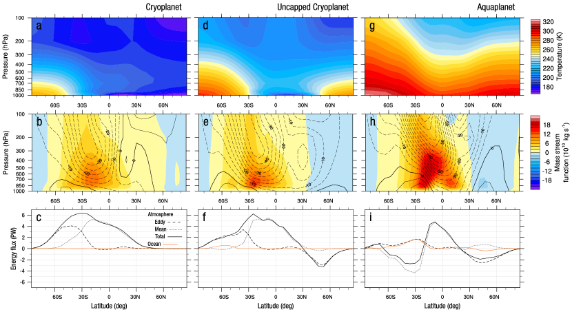
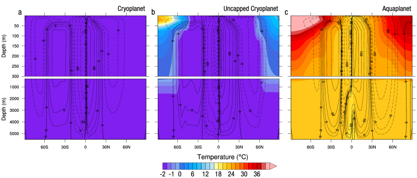
Figure 1: Stable climate states simulated using a coupled atmosphere-ocean-sea ice model (version OD) at high obliquity ($\epsilon=90$°). Shown are ten-year monthly means for January. a-c: Cryoplanet (relative stellar irradiance $\tilde{S}=0.7$). d-f: Uncapped Cryoplanet ($\tilde{S}=0.94$). g-i: Aquaplanet ($\tilde{S}=1.0$). Shown are (a,d,g) the zonal-mean atmospheric temperature (color interval 5 K), (b,e,h) mass stream function (color interval $2\times 10^{10}$ kg s^-1, positive for clockwise overturning) and zonal-mean zonal wind (contour interval 5 m s^-1, positive for westerlies), and (c,f,i) the meridional atmospheric energy flux, consisting of the eddy and mean circulation contributions, and the meridional ocean heat flux. Positive values represent a northward flux.

Figure 2: Ocean component of the stable climate states at high obliquity ($\epsilon=90$°) shown in Fig. 2. a: Cryoplanet ($\tilde{S}=0.7$). b: Uncapped Cryoplanet ($\tilde{S}=0.94$). c: Aquaplanet ($\tilde{S}=1.0$). Shown are the zonal-mean ocean temperature (color interval: 0.5℃ for $<0$℃ and 2℃ for $\geq 0$℃) and the meridional overturning (contour interval are in Sv: $0,\pm 2.5,\pm 5,\pm 10,\pm 20,\pm 50,\pm 100,\pm 150,\pm 200$; positive for clockwise overturning).

At high obliquity $\epsilon$, the fully dynamical model OD exhibits three different climate states depending on the strength of the stellar irradiance. This is shown for $\epsilon=90$° where for increasing values of $\tilde{S}$, the Cryoplanet, Uncapped Cryoplanet, and the Aquaplanet are found (Fig. 2). This is consistent with, and confirms earlier simulations using the simpler model version with only a slab ocean (OS, Kilic et al., 2017a). We note, however, that the Near Cryoplanet, as state with seasonally open polar oceans, is not obtained with the OD version. Nevertheless, this similar solution structure at $\epsilon=90$° indicates that OS is a reasonable emulator of OD. This will be corroborated further below.

The main characteristics of the climate states are shown in Fig. 2 for January. The atmosphere of the Cryoplanet is very cold due to the sea ice albedo reflecting large amounts of the stellar energy flux back to space. Only the polar atmosphere facing the star is significantly warmer than the remaining part of the planet highlighting the strong seasonality of the cryoplanet climate. The Uncapped Cryoplanet has an ice cover that is confined to the low latitudes, and both polar areas are ice free. This is due to the underlying open ocean that absorbs heat during the summer months which keeps the ocean surface ice free in the winter. Therefore, both polar atmospheres are warm throughout the year. In the aquaplanet state surface temperatures are warm at all latitudes with a seasonal cycle that is damped by the presence of the underlying ocean.

The zonal circulation in the atmosphere shows a strong thermally-driven easterly jet in all three states in the summer hemisphere (Fig. 2). Still, differences in structure, strength and mechanisms are present. In the case of the Cryoplanet and Uncapped Cryoplanet, the overturning circulation of the atmosphere is driven by both eddy and mean atmospheric energy fluxes (for further details see Kilic et al., 2017a). For the Aquaplanet, the overturning circulation consists of two thermally direct driven cells in the area of 60°S to 20°N. The thermally indirect atmospheric circulation in the winter hemisphere of the Aquaplanet is caused by the dominant northward eddy heat flux (Fig. 2i).

Apart from the strong easterly jet, the zonal circulation in the atmosphere differs in structure and strength in the three states. Meridionally, all three states feature a thermally direct one-cell circulation in the summer hemisphere. In the case of the Cryoplanet and Uncapped Cryoplanet the underlying mechanism driving the atmospheric circulation is the same (for further details see Kilic et al., 2017a).

Ocean circulation contributes very little to the meridional heat flux when the planet is completely or partly ice covered (Fig. 2c,f). Conversely, there is a substantial ocean heat flux in the summer hemisphere towards the equator in the case of the Aquaplanet (Fig. 2i).

Figure 2 shows the zonal-mean temperature and meridional overturning in the ocean for the simulations given in Fig. 2. Below 100 m depth, the ocean temperature is nearly symmetric about the equator despite the strong seasonal variability of the atmosphere at $\epsilon=90$° (Fig. 2). This is due to the large heat capacity of the ocean and the associated thermal adjustment time on the order of 10³ years.

In the case of the cryoplanet and the uncapped cryoplanet states, the ocean temperature below the sea ice cover is close to the freezing point and features very small meridional and vertical gradients. Therefore, the meridional overturning is mainly caused by the Ekman transport driven at the surface by a combination of wind stress and its transfer through sea ice (Fig. 2a,b). Overturning strengthens towards the equator because Ekman transport scales with the inverse of the Coriolis parameter. The ocean temperature of the Uncapped Cryoplanet reflects the meridional structure of surface temperature in the atmosphere with the warmest water in the ice-free polar areas (Fig. 2b). The polar thermocline reaches to a depth of about 400 m in winter and less than 100 m in summer. Under the sea ice, vertical temperature gradients are very small, which explains the very small meridional ocean heat flux despite a substantial meridional overturning circulation (Fig. 2c,f).

In the case of the aquaplanet state, the meridional overturning in the ocean is additionally driven by the density gradients as is evident from the large vertical and meridional temperature (and salinity) gradients (Fig. 2c). This leads to a substantial equatorward meridional heat flux in the ocean in the summer hemisphere (Fig. 2i).

4 Stable regimes and Hysteresis

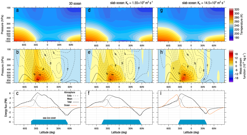
Figure 3: Same as Fig. 2 but for three uncapped cryoplanet states showing ten-year monthly means for January with $\epsilon=90$° and $\tilde{S}=0.94$: (a-c) OD configuration as in Fig. 2. (d-f) OS configuration $K_{h}=1.55\cdot 10^{4}$ m² s^-1. (g-i) OS configuration with $K_{h}=14.5\cdot 10^{4}$ m² s^-1. In the bottom panels, the blue areas indicate the sea ice cover. Note that the OS configuration (d-f) is a good emulator of the dynamical model configuration OD. In OS the meridional ocean heat flux can be increased by increasing $K_{h}$ (i).

An earlier study suggested that a dynamical ocean circulation would not permit stable climate states with a perennial equatorial ice cover, i.e., an uncapped cryoplanet state, under high obliquity conditions (Ferreira et al., 2014). They started their simulations from an aquaplanet configuration. Not inconsistent with this finding, our earlier simulations using OS (Kilic et al., 2017a) showed that an uncapped cryoplanet state could only be reached from a cryoplanet but not from an aquaplanet configuration. Here we find that such a state may also in a fully dynamical atmosphere-ocean model (OD). In order to investigate the sensitivity of the uncapped cryoplanet state to the strength of the meridional ocean heat transport we now use OS as an emulator. In OS the relative importance of the ocean heat transport can be varied by the horizontal diffusivity $K_{h}$ of the slab ocean. This is illustrated in Fig. 3 for the uncapped cryoplanet state at $\epsilon$ = 90° and $\tilde{S}=0.94$. With a horizontal diffusivity of $K_{h}=1.55\cdot 10^{4}$ m² s^-1 the emulator OS reproduces the seasonal distribution of atmospheric temperature, the zonal and meridional atmospheric circulations, as well as the meridional heat fluxes in the ocean and the atmosphere, including the eddy and mean components. Also the equatorial sea ice cover simulated by the emulator is in quantitative agreement with the results from the dynamical atmosphere-ocean model (Fig. 3a-c v.s. d-f).

In the emulator we can strengthen the meridional ocean heat flux by simply increasing $K_{h}$. This simulates a case in which the effect of the distribution of heat via the ocean circulation becomes more important. If the horizontal diffusivity is increased by almost an order of magnitude to $K_{h}=14.5\cdot 10^{4}$ m² s^-1, the peak meridional ocean heat flux towards the ice edges reaches a magnitude similar to that in the atmosphere (Fig. 3i). In spite of this large supply of heat to the ice edge, the Uncapped Cryoplanet remains a steady state. However, a slight further increase of the slab ocean diffusivity $K_{h}$, and in consequence of the meridional ocean heat flux, causes the crossing of a tipping point which triggers the irreversible melting of the equatorial sea ice with subsequent transition to the aquaplanet state. It is the ocean heat flux towards the ice edge that eventually destroys the equatorial ice belt.

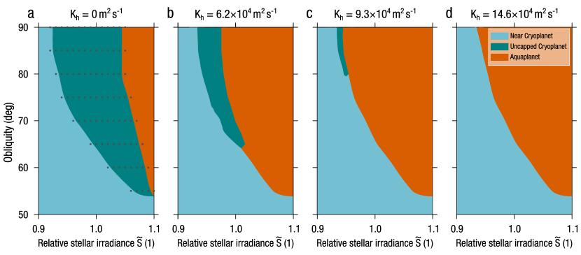
Figure 4: Regions of three distinct stable climate states in obliquity-irradiance space using a dynamical atmosphere coupled to slab ocean and sea ice model (OS configuration). All simulations are started from a cryoplanet initial state. The dots in panel (a) indicate the sampled locations in obliquity-irradiance space. Increasing diffusivities $K_{h}$ of the slab ocean were used for these simulations to determine the effect on the location of the region boundaries of the uncapped cryoplanet state. The area where the Uncapped Cryoplanet is stable is largest in the configuration of a swamp ocean ($K_{h}=0$ m² s^-1, panel a) and decreases with increasing $K_{h}$. If $K_{h}$ exceeds a critical value ($K_{h}\geq 14.6\cdot 10^{4}$ m² s^-1), only the Aquaplanet and the Near Cryoplanet remain as stable states (panel d).

With the OS emulator we now explore the region of stability for the uncapped cryoplanet state in the $\epsilon$-$\tilde{S}$-$K_{h}$-parameter space. In Fig. 4 we show the change of the steady state regions with increasing $K_{h}$. Sampling of the parameter space using the emulator OS permits us to locate the state boundaries. In the range from $K_{h}=0$ m² s^-1 (no meridional heat flux in the ocean) to $K_{h}=9.6\cdot 10^{4}$ m² s^-1 we find three different equilibrium states. Generally, for high $\tilde{S}$, no ice is sustained and an Aquaplanet results; for lower $\tilde{S}$ a Near Cryoplanet is simulated which has a seasonally open polar area. In between, the Uncapped Cryoplanet is found which has perennially open polar areas and an equatorial ice belt. This is a stable state that is robust against rather large changes of horizontal diffusivity $K_{h}$ around the standard value. The choice of the standard $K_{h}=1.55\cdot 10^{4}$ m² s^-1 for the OS model is based on present-day conditions, i.e. $\tilde{S}=1$ and $\epsilon=23.4$°, and agreement with the large-scale atmospheric properties and dynamics (Kilic et al., 2017a). By increasing $K_{h}$ by almost an order of magnitude this state remains stable (Fig. 4c), although the extent of the region of existence reduces significantly.

For larger $K_{h}$, and hence stronger ocean heat transport, the uncapped cryoplanet region is confined to a narrower range of $\tilde{S}$ and higher obliquity. For $K_{h}=14.5\cdot 10^{4}$ m² s^-1 the uncapped cryoplanet remains a stable state at just $\epsilon$=90° and $\tilde{S}=0.94$ (Fig. 3g-i). For even larger $K_{h}$ this state is no longer realized, as test simulations at $K_{h}=20\cdot 10^{4}$ m² s^-1 have revealed. This defines a critical threshold of $K_{h}$ beyond which the meridional ocean heat flux is too large to sustain equatorial ice. Our simulations suggest that this threshold is at about $14.6\cdot 10^{4}$ m² s^-1 for the present model configuration.

For the swamp ocean that only acts as a heat storage ($K_{h}=0\,$m² s^-1), the stable regime for the uncapped cryoplanet state reaches its largest extent. This highlights the sensitivity of the equilibrium states on the repartitioning of meridional energy fluxes. With increasing dominance of the ocean transport, the uncapped cryoplanet state is sustained in only a small area of the parameter space before it loses stability. Therefore, it depends on the details of the ocean circulation how many different equilibrium states of planetary climate can be realized.

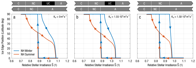
Figure 5: Hysteresis loops of the northern winter and summer ice edge positions in the Northern Hemisphere as the relative stellar irradiance $\tilde{S}$ is increased or decreased. Simulations are carried out with the OS version at $\epsilon=90$° for three values of $K_{h}$ as shown in panels (a), (b) and (c). The upper horizontal gray bars above the panels indicate the equilibrium states that are visited successively when increasing $\tilde{S}$: C Cryoplanet (complete ice cover), NC Near Cryoplanet (seasonally open polar oceans), UC Uncapped Cryoplanet (perennially open polar oceans), and A Aquaplanet (ice free). The sequence of equilibria is reversed when decreasing $\tilde{S}$, as shown in the lower horizontal gray bars, except that no UC is simulated because of a tipping point in the winter ice edge position. The shape of the hysteresis loops for the ice edge positions, and hence the sequence of equilibrium states, depends on $K_{h}$; for large $K_{h}$ (panel c), no UC is simulated in either direction of $\tilde{S}$ change. For decreasing $\tilde{S}$ no UC is simulated independent of the value of $K_{h}$.

In order to illustrate how the initial condition influences the stable equilibrium, we select obliquity $\epsilon=90$° and use the OS version for three cases of $K_{h}$. By slowly increasing $\tilde{S}$ by $10^{-4}$ yr^-1, equilibrium states are visited successively. The states can be characterized by the latitudinal position of their northern ice edges in winter and summer, respectively (Fig. 5). First, simulations start at low stellar irradiance $\tilde{S}=0.7$ in the fully ice covered cryoplanet state. Once the northern edge of the summer sea ice cover moves southward the polar ocean becomes seasonally ice free, while winter sea ice still extends from the equator to the pole. This is the near cryoplanet state. Upon further increasing $\tilde{S}$, also the northern edge of the winter sea ice cover begins to move equatorward and the polar oceans now remain open throughout the year. This is the Uncapped Cryoplanet that is stable for a considerable range of stellar irradiance. The gradual equatorward movement of both northern ice edge latitudes when irradiance becomes stronger eventually produces an ice free ocean, the aquaplanet state. Note that in Fig. 5c the hysteresis branch for the winter sea ice edge transition from 90° to 0° is not vertical which would suggest a very narrow range of an uncapped cryoplanet. However, such states are only transient, and the finite slope of the hysteresis branch is caused by the rate of change of $\tilde{S}$ being faster than the approach to the steady state of the Aquaplanet.

Second, when $\tilde{S}$ is reduced again to below 0.9, a tipping point for both the winter and summer ice edge is reached simultaneously. While the northern edge position of the summer sea ice cover arrests at about 50° latitude and then moves poleward, the winter ice edge position jumps directly to 90°, i.e., the planet makes a transition from a perennially ice free to a completely ice covered ocean during winter. Therefore, no uncapped cryoplanet state is found when simulations start from an Aquaplanet. An important result is that irrespective of $K_{h}$ the uncapped cryoplanet state is not reached when starting from an Aquaplanet. This suggests that the particulars of the ocean model are not the main reason why other studies did not find stable states with an equatorial ice belt at high obliquity (Chandler & Sohl, 2000; Williams & Pollard, 2003; Ferreira et al., 2014; Jenkins, 2000, 2001, 2003), but rather the albedo effect afforded by the initial conditions.

5 Conclusion

We have shown using a dynamical atmosphere-ocean climate model that the state with an equatorial ice belt, the Uncapped Cryoplanet, is a stable state at high obliquity for a range of stellar irradiance. This confirms our earlier findings that used a simpler configuration consisting of an atmospheric model coupled to a slab ocean (Kilic et al., 2017a). Our results apply to both the slab and the dynamical ocean versions. Furthermore, our simulations using the simpler configuration as an emulator model provide insight into the stability of the uncapped cryoplanet state and its dependence on initial conditions. With increasing importance of the ocean heat transport the equatorial ice cover shrinks in latitudinal extent until it becomes unsustainable. This marks a critical point where a transition to the aquaplanet state occurs. Transient simulations in which the stellar irradiance is slowly increased or decreased, demonstrate that the Uncapped Cryoplanet only is reached from more glaciated conditions, e.g. the cryoplanet or the near cryoplanet states, but not from less glaciated states. This result does not depend on the presence or absence of a meridional ocean heat flux.

This is reminiscent of robust hysteresis behavior and multiple equilibria in the non-linear atmosphere-ice-ocean system, as demonstrated earlier (Lucarini et al., 2013; Kilic et al., 2017a; Rose et al., 2017). We have shown that the shape of the hysteresis depends on model parameters. By inference, one would expect that the position and shape of a hysteresis loop is also model dependent. Ferreira et al. (2014) concluded that an equatorial ice belt is unlikely to exist. The difference to our finding could be due to two reasons. First, their model consisted of an ocean component based on primitive equations which is dynamically more realistic than the LSG formulation which neglects the non-linear momentum advection. This would likely result in a different hysteresis structure. Second and more importantly, they initialized their simulations only from an aquaplanet state. Hence, the Uncapped Cryoplanet may also be realized in their model if their simulations had started from a more glaciated state. Further exploration of the solution space of that model is therefore warranted. More generally, we suggest that exoplanet research would highly benefit from coordinated model intercomparison efforts, as have now become the standard in the Earth System Model community (Eyring et al., 2016).

We emphasize that our simulations are idealized and only represent a first approach to the investigation of stable climate regimes under high obliquity. This is justifiable in the absence of more detailed information on exoplanet surface conditions and configurations. For instance, during an exoplanet’s evolution tectonic processes could form ocean basins and land masses that would fundamentally alter the ocean circulation and the associated meridional heat flux. While land masses would provide a solid ground for growing ice masses and enhance the albedo feedbacks, they would also be more susceptible to heating due to their smaller heat capacity. Therefore, it is currently not possible to assess the consequence of different land-ocean configurations on the distribution of stable climate states on a high-obliquity exoplanet. Further observational information and simulations are required to explore such questions.

In conclusion, our simulations demonstrate that the irradiation history of an exoplanet is the primary determinant of whether an equatorial ice belt would occur as a climate state during its evolution. Once the planet has reached an ice free state, it seems unlikely that it would reach an uncapped cryoplanet again at some later stage, unless another planet-scale glaciation has occurred. This finding is relevant for understanding habitable conditions over the entire climatic evolution of an exoplanet.

References

- Abe et al. (2011) Abe, Y., Abe-Ouchi, A., Sleep, N. H., & Zahnle, K. J. 2011, Astrobiology, 11, 443, doi: 10.1089/ast.2010.0545
- Armstrong et al. (2014) Armstrong, J. C., Barnes, R., Domagal-Goldman, S., et al. 2014, Astrobiology, 14, 277, doi: 10.1089/ast.2013.1129
- Chandler & Sohl (2000) Chandler, M. A., & Sohl, L. E. 2000, Journal of Geophysical Research: Atmospheres, 105, 20737, doi: 10.1029/2000JD900221
- Eyring et al. (2016) Eyring, V., Bony, S., Meehl, G. A., et al. 2016, Geoscientific Model Development, 9, 1937, doi: 10.5194/gmd-9-1937-2016
- Ferreira et al. (2014) Ferreira, D., Marshall, J., O’Gorman, P. A., & Seager, S. 2014, Icarus, 243, 236, doi: 10.1016/j.icarus.2014.09.015
- Hertwig et al. (2015) Hertwig, E., Lunkeit, F., & Fraedrich, K. 2015, Theoretical and Applied Climatology, 121, 459, doi: 10.1007/s00704-014-1226-8
- Jenkins (2000) Jenkins, G. S. 2000, Journal of Geophysical Research: Atmospheres, 105, 7357, doi: 10.1029/1999JD901125 EOLEOL
- Jenkins (2001) —. 2001, Journal of Geophysical Research: Planets, 106, 32903, doi: 10.1029/2000JE001427
- Jenkins (2003) —. 2003, Journal of Geophysical Research: Amospheres, 108, 4118, doi: 10.1029/2001JD001582
- Kaspi & Showman (2015) Kaspi, Y., & Showman, A. P. 2015, The Astrophysical Journal, 804, 60, doi: 10.1088/0004-637X/804/1/60
- Kilic et al. (2017a) Kilic, C., Raible, C. C., & Stocker, T. F. 2017a, The Astrophysical Journal, 844, 147, doi: 10.3847/1538-4357/aa7a03
- Kilic et al. (2017b) Kilic, C., Raible, C. C., Stocker, T. F., & Kirk, E. 2017b, Planetary and Space Science, 135, 1, doi: 10.10164/j.pss.2016.11.001
- Laskar et al. (1993) Laskar, J., Joutel, F., & Robutel, P. 1993, Nature, 361, 615, doi: 10.1038/361615a0
- Levrard & Laskar (2003) Levrard, B., & Laskar, J. 2003, Geophysical Journal International, 154, 970, doi: 10.1046/j.1365-246X.2003.02021.x EOLEOL
- Lucarini et al. (2013) Lucarini, V., Pascale, S., Boschi, R., Kirk, E., & Iro, N. 2013, Astronomische Nachrichten, 334, 576, doi: 10.1002/asna.201311903
- Lunkeit et al. (2011) Lunkeit, F., Borth, H., Böttinger, M., et al. 2011, Planet Simulator - Reference Manual Version 16, Meteorological Institute, University of Hamburg
- Maier-Reimer et al. (1993) Maier-Reimer, E., Mikolejewicz, U., & Hasselmann, K. 1993, Journal of Physical Oceanography, 23, 731, doi: 10.1175/1520-0485(1993)023<0731:MCOTHL>2.0.CO;2
- Pierrehumbert (2010) Pierrehumbert, R. T. 2010, Principles of Planetary Climate (Cambridge University Press, 674 pp), 647 pp.
- Pierrehumbert et al. (2011) Pierrehumbert, R. T., Abbot, D. S., Voigt, A., & Koll, D. 2011, Annual Review of Earth and Planetary Sciences, 39, 417, doi: 10.1146/annurev-earth-040809-152447
- Prange et al. (2003) Prange, M., Lohmann, G., & Paul, A. 2003, Journal of Physical Oceanography, 33, 1707, doi: 10.1175/2389.1
- Rose et al. (2017) Rose, B. E. J., Cronin, T. W., & Bitz, C. M. 2017, The Astrophysical Journal, 846, 28, doi: 10.3847/1538-4357/aa8306
- Williams & Pollard (2003) Williams, D. M., & Pollard, D. 2003, International Journal of Astrobiology, 2, 1, doi: 10.1017/S1473550403001356
- Williams (1975) Williams, G. E. 1975, Geological Magazine, 112, 441, doi: 10.1017/S0016756800046185