Diffusion rate of windtree models and Lyapunov exponents

Abstract.

Consider a windtree model with several parallel arbitrary right-angled obstacles placed periodically on the plane. We show that its diffusion rate is the largest Lyapunov exponent of some stratum of quadratic differentials and exhibit a new general strategy to compute the generic diffusion rate of such models. This result enables us to compute numerically the diffusion rates of a large family of models and to observe its asymptotic behaviour according to the shape of the obstacles.

1. Introduction.

The windtree model was first introduced by Paul and Tatiana Ehrenfest in 1912 [EE90] as part of statistical physics investigations. In this book they set a simplified model for non interacting light particles moving around massive particles that do not move but on which the light particles bounce with elastic collision. We classically refer to the light particles as the wind and the static ones as trees. The motivation of the two physicists was to understand the kinetic behaviour of such a system. They asked, among others, the following question: for a generic disposition of square trees orientated in the same direction, does the speed of $K$ light particles equidistributes asymptotically in the $4$ possible directions ?

Plenty of questions have been studied on this model, in particular for the $\mathbb{Z}^{2}$-periodic case with square obstacles. The results feature alternatively elements of chaotic and periodic behaviour. In [HW80] was proven on the one hand recurrence of the billiard flow and on the other hand abnormal diffusion for special dimensions of the obstacles, [FU14] showed genericity of non-ergodic behaviour, and its diffusion rate was computed to be $2/3$ in [DHL14]. A positive answer to the original question has only been provided very recently by [MST18].

In parallel a similar model with smooth convex obstacles has been studied by a large amount of mathematicians throughout the twentieth century (see e.g. [BS81] or [SV04]). In this case, the billiards satisfy some hyperbolicity property and the behaviour of its flow is closely related to a Brownian motion.

A good tool to check if a polygonal windtree model has such an hyperbolic behaviour is provided by the diffusion rates which should be $1/2$ in the case of Brownian-like motions. In particular the result of [DHL14] breaks any hope to apply directly methods of the smooth convex case to the rectangular model. The question is still open in the case of asymptotic of polygonal shapes approaching smooth convex ones, for example with the circle : is the diffusion rate of periodic windtree models with regular $n$-gons going to $1/2$ when $n$ goes to $\infty$ ? We hope that developing methods to compute these diffusion rates in more general settings provide a first step to understanding this asymptotic and the non-convex obstacles cases.

The arguments of [DHL14] relies on a remarkable correspondence between the diffusion rate of an infinite periodic billiard table and the Lyapunov exponent of an associated translation surface. This computation was generalised in [DZ15] to any $\mathbb{Z}^{2}$-periodic windtree which trees have only right angles and are horizontally and vertically symmetric. In every of these cases, the corresponding Lyapunov exponent belongs to some $2$ dimensional subbundle of the Hodge bundle. Moreover in all of these cases the Lyapunov exponent is rational and can be computed using some geometric arguments.

In this article we describe a general strategy to exhibit the Lyapunov exponent of some locus in a stratum that corresponds to the diffusion rate of a given periodic windtree model. It relies on two main ingredients : the first one is to identify a common orbit closure of almost all translation surfaces associated to a family of windtree tables; the second one is to find an irreducible subbundle of the Hodge bundle on this locus which top Lyapunov exponent is exactly the diffusion rate. The tools for the first craft are given by recent results of [EMM15], [Wri14] and [Wri15] and are introduced in subsection 4.1. For the second one, we show an additional lemma to the work of [CE15] which yields the diffusion rate for any translation surface in a generic direction.

We apply this method to the case of periodic windtree with several obstacles in its fundamental domain. Pick a family of $n\geq 2$ rectangular obstacles in a square, and repeat this table $\mathbb{Z}^{2}$-periodically in the plane. We show the following theorem,

Theorem.

The diffusion rate for almost every such windtree model, in almost every direction is equal to the top Lyapunov exponent of $\mathcal{Q}(1^{4n})$.

Now take more general obstacles again with right angles, if $n$ is the number of obstacles ans $p$ the total number of inward (concave) right angles in all the obstacles, we have a similar result,

Theorem.

The diffusion rate for almost every such windtree model, in almost every direction is equal to the top Lyapunov exponent of $\mathcal{Q}(1^{4n+p},-1^{p})$.

In the last section we discuss the value of these exponents running numerical experiments with a Sage code developed by the author in a collaborative project [D⁺16]. These experiments give strong evidences that the family we have introduced above can approach arbitrarily close any diffusion rate between $1/2$ and $0$. In particular it goes to $1/2$ (i.e. the diffusion rate of the Brownian motion) when the number of obstacles goes to infinity.

2. Translation surfaces

2.1. Definition

A translation surface is a surface whose change of charts are translations. Such a surface is endowed with a flat metric (the pull-back of the canonical metric on $\mathbb{R}^{2}$) and a canonical direction.

One way to think of these translation surfaces is by gluing sides of a polygon via translations. Let $P$ be a polygon with $2k$ edges and let $z_{1},\dots,z_{2k}$ be complex numbers associated to the vectors of its sides. Assume that $z_{i}=z_{k+i}$, we glue the sides $z_{i}$ and $z_{k+i}$ and obtain a flat surface with conical singularities of angle multiples of $2\pi$.

We can define similar structures allowing the change of charts to be also translations composed with $-\mathrm{Id}$. The class of surfaces we obtain are called half-translation surfaces.

Using triangulations Veech showed in [Vee93] that this is a general construction with a notion of pseudo-polygons (in a much wider class of structures). The complex numbers $(z_{i})_{1\leq i\leq k}$ (defined up to a sign in the case of half-translation surfaces) induce local coordinates in the moduli space of such structures, we call them period coordinates. We will introduce them as periods of abelian differentials below.

2.1.1. Differentials and Moduli spaces

There is a one-to-one correspondence between compact translation surfaces and Riemann surfaces equipped with a non-zero holomorphic $1$-form. As well as between compact half-translation surfaces and Riemann surfaces equipped with quadratic differentials.

For $g\geq 1$ let $\alpha$ and $\beta$ be partitions of $2g-2$ and $4g-4$. The strata $\mathcal{H}(\alpha)$ and $\mathcal{Q}(\beta)$ are defined to be the sets of $(S,\omega)$ and $(S,q)$ where $S$ is a genus $g$ closed Riemann surface, $\omega$ is a holomorphic $1$-form on $S$, $q$ is a quadratic differential on $S$, and their zeros multiplicities are given by $\alpha$ and $\beta$. The conical points in a translation surface correspond to the zeros of the differential. If $d$ is the multiplicity of the zero, the angle is equal to $2(d+1)\pi$ (and $(d+2)\pi$ for half-translation surfaces).

Given a translation surface $(S,\omega)$, let $\Sigma\subset S$ be the set of zeros of $\omega$. Pick a basis $\{\xi_{1},\dots,\xi_{n}\}$ for the relative homology group $H_{1}(S,\Sigma;\mathbb{Z})$. The map $\Phi:\mathcal{H}(\alpha)\to\mathbb{C}^{n}$ defined by

$$\Phi(S,\omega)=\left(\int_{\xi_{1}}\omega,\dots,\int_{\xi_{n}}\omega\right)$$

redefines local period coordinates with translation as change of charts as above.

There is a natural action of $\mathrm{GL}(2,\mathbb{R})$ on connected components of strata coming from linear action of $\mathrm{GL}(2,\mathbb{R})$ on $\mathbb{R}^{2}$ in charts. For any translation surface in a stratum, its orbit closure via this action is some affine invariant manifold of the stratum : it is defined in local period coordinates by linear equations. They are endowed with a canonical measure supported on these surfaces called affine measures [EM13], [EMM15].

2.1.2. Translation cover

To any primitive half-translation surfaces $S$ we associate its translation cover $\hat{S}$ corresponding to the subgroup of the fundamental group with holonomy equal to $-1$. It is a double cover. We endow $\hat{S}$ with the pulled-back metric of $S$ which defines a translation surface structure for $\hat{S}$.

From a differential geometric point of view, we constructed a double cover of $S$ on which the quadratic differential $q$ can be written $\omega^{2}$ where $\omega$ is a holomorphic $1$-form.

Let $(S,q)$ be a half-translation surface in $\mathcal{Q}(m_{1},\dots m_{d})$, $\hat{S}$ its translation cover and $\hat{\Sigma}$ the preimage of its singular points. Following [AEZ16], assume there is a basis $\{a_{1},b_{1},\dots,a_{g},b_{g}\}$ of $H_{1}(S;\mathbb{Z})$ which has trivial linear holonomy (this exists as long as there is a zero with odd multiplicity) and let $\gamma_{1},\dots,\gamma_{d-2}$ be primitive non crossing elements of $H_{1}(S,\Sigma;\mathbb{Z})$ representing a path from $P_{i}$ to $P_{i+1}$ where $\{P_{1},\dots,P_{d}\}=\Sigma$.

Given a saddle connection or an absolute cycle with trivial linear holonomy $\gamma$, let $\gamma^{\prime},\gamma^{\prime\prime}$ be its $2$ lifts in $\hat{S}$ endowed with the orientation inherited from $\gamma$. Then we introduce

$$\hat{\gamma}:=\gamma^{\prime}-\gamma^{\prime\prime}.$$

By definition $\hat{\gamma}$ belongs to $H^{-}_{1}(\hat{S},\hat{\Sigma};\mathbb{C})$ the $-1$-eigenspace of the linear automorphism induced by the deck involution of the double cover.

Proposition 1.

The family $\{\hat{a}_{1},\hat{b}_{1},\dots,\hat{a}_{g},\hat{b}_{g},\hat{\gamma}_{1},\dots,\hat{\gamma}_{d-2}\}$ is a basis of $H^{-}_{1}(\hat{S},\hat{\Sigma};\mathbb{C})$.

The dual family of $\{\hat{a}_{1},\hat{b}_{1},\dots,\hat{a}_{g},\hat{b}_{g},\hat{\gamma}_{1},\dots,\hat{\gamma}_{d-2}\}$ forms a basis of the anti-invariant $1$-forms,

$$H^{1}_{-}(\hat{S},\hat{\Sigma};\mathbb{C})\subset H^{1}(\hat{S},\hat{\Sigma};\mathbb{C})$$

where the relative cohomology is a local chart for some abelian stratum $\mathcal{H}(\alpha)$. This period is twice the polygonal periods we defined above up to a sign.

This is the basis we will be using to express equations of billiard families.

2.2. Windtree tables

Let $P$ a filled polygon which does not self-intersect will stand for the shape of the obstacles in our infinite billiard. Consider the plane $\mathbb{R}^{2}$ on which we place $P$ periodically centered at each point of a lattice $\Lambda$ as scatterers such that copies do not overlap. We denote the space consisting of the plane to which we removed the inside of every obstacle by $\mathcal{W}(P,\Lambda)$.

Definition 1.

We call $\mathcal{W}(P,\Lambda)$ a $\Lambda$-periodic windtree table with obstacle $P$.

Our purpose here is to understand the billiard flow on this infinite table and its asymptotic speed. We denote the billiard flow by

$$\phi_{t}^{\theta}:\mathcal{W}(P,\Lambda)\mapsto\mathcal{W}(P,\Lambda).$$

For $p\in\mathcal{W}(P,\Lambda)$ the point $\phi_{t}^{\theta}(p)$ is the position of the flow after time $t$ starting from $p$ in direction $\theta$, which moves in straight lines until it encounters an obstacle on which it bounces according to Snell-Descartes law of reflection.

Definition 2.

In a windtree table $\mathcal{W}(P,\Lambda)$ for $d$ the euclidian distance on $\mathbb{R}$, $p\in\mathcal{W}(P,\Lambda)$ and $\theta\in[0,2\pi)$ the diffusion rate is the limit

$$\limsup_{t\to+\infty}\frac{\log d(p,\phi_{t}^{\theta}(p))}{\log t}.$$

2.2.1. Associated flat surface

As the billiard table $\mathcal{W}(P,\Lambda)$ is $\Lambda$-periodic, we may consider its quotient

$${\raisebox{1.99997pt}{$\mathcal{W}(P,\Lambda)$}\left/\raisebox{-1.99997pt}{$\Lambda$}\right.}\simeq{\raisebox{1.99997pt}{$\mathbb{R}^{2}$}\left/\raisebox{-1.99997pt}{$\Lambda$}\right.}-\mathring{P}=:\mathcal{T}_{\Lambda}(P)$$

which corresponds to playing billiard in a torus with one copy of the obstacle $P$ placed in it. Then we associate to it a flat surface on which the linear flow corresponds to the billiard flow.

Take two copies of $\mathcal{T}_{\Lambda}(P)$ and glue the two copies of each side of $P$ using an isometry fixing the tangent vector and inverting the normal vector (the axial symmetry along this side). Now when the flow is bouncing in the billiard, the geodesic flow of the flat surface is simply changing of copy in the surface.

The gluing maps are changing orientation, hence in order for this surface to be a flat surface as defined above we choose as a convention two opposite orientations for the two copies. The change of charts now preserves orientation and is in $\operatorname{Iso}^{+}(\mathbb{C})$. We denote this flat surface by $S(P,\Lambda)=S$.

For each triple $(p,\theta,t)\in S\times[0,2\pi)\times\mathbb{R}_{+}$ we define an element $\gamma_{t}^{\theta}(p)\in H^{1}(S;\mathbb{Z})$ as follows. Consider the geodesic segment of lengths $t$ starting from $p$ in the direction $\theta$ and close it by a small piece of curve that does not cross $h_{\kappa}$ and $v_{\kappa}$. The curve used to close the segment can be chosen to be uniformly bounded.

Let $h,v$ be a horizontal and vertical simple loop in $\mathcal{T}_{\Lambda}(P)$ that generate the homology of the torus. Let $h^{S}=h_{1}-h_{2}$ and $v^{S}=v_{1}-v_{2}$ where $h_{1},h_{2}$ (resp $v_{1},v_{2}$) are the two lifts of $h$ (resp. $v$) in $S$. And let a $f\in H^{1}(S;\mathbb{Z}^{2})$ be a cocycle dual of $(h^{S},v^{S})$ with respect to the intersection form.

The proposition below shows that the diffusion rate of a particle in a windtree table $\mathcal{W}(P,\Lambda)$ can be reduced to the study of the pairing of the approximate geodesic flow on $S$ with $f$.

Proposition 2 (1 in [DHL14]).

The diffusion rate of $\phi_{t}^{\theta}(\tilde{p})$ is equal to

$$\limsup_{t\to+\infty}\frac{\log\left|\left<f,\gamma_{t}^{\theta}(p)\right>\right|}{\log t}$$

when $p$ and $\tilde{p}$ project to the same point on $\mathcal{T}_{\Lambda}(P)$.

3. Lyapunov exponents

In the previous section, we have seen that the diffusion rate on a windtree table is related to the asymptotic pairing of a cohomology class with a modified linear flow on the associated translation surface. We will consider throughout this section a translation $S$ in some abelian stratum $\mathcal{H}(\alpha)$ which $\mathrm{SL}(2,\mathbb{R})$-orbit closure is the affine invariant subspace $\mathcal{M}\subset\mathcal{H}(\alpha)$ and $\nu_{\mathcal{M}}$ its invariant measure.

The following theorem relates the diffusion rate with a Lyapunov exponent,

Theorem (2 in [DHL14]).

Let $F_{1}\supset F_{2}\supset\dots\supset F_{k}$ be the Oseledets flag decomposition of the Kontsevich-Zorich cocycle on $\mathcal{M}$, and $\lambda$ be its top Lyapunov exponent. For every $\nu_{\mathcal{M}}$-Oseledets generic translation surface $S\in\mathcal{H}(\alpha)$, for every point $p\in S$ with infinite forward orbit, for all $f\in F_{1}\setminus F_{2}$,

$$\limsup_{t\to+\infty}\frac{\log|\left<f,\gamma_{t}(p)\right>|}{\log t}=\lambda.$$

In [CE15] is proven that any translation surface $S\in\mathcal{H}(\alpha)$ such that its $\mathrm{SL}(2,\mathbb{R})$-orbit closure is $\mathcal{M}$ is Oseledets generic in Lebesgue-almost every direction. In particular they show the following theorem,

Theorem 1.

1.5 in [CE15] Fix $S\in\mathcal{H}_{1}(\alpha)$ and let $\mathcal{M}=\overline{\mathrm{SL}(2,\mathbb{R})\cdot S}$ the smallest affine invariant manifold containing $S$, let $V$ be a $\mathrm{SL}(2,\mathbb{R})$ invariant subbundle of the Hodge bundle which is defined and continuous on $\mathcal{M}$. Let $A_{V}:\mathrm{SL}(2,\mathbb{R})\times\mathcal{M}\rightarrow V$ denote the restriction of the Kontsevich-Zorich cocycle to $V$ and suppose that $A_{V}$ is strongly irreducible with respect to the affine measure $\nu_{\mathcal{M}}$ whose support is $\mathcal{M}$. Then, for almost every $\theta\in[0,2\pi)$,

$$\lim_{t\to\infty}\frac{\log||A_{V}(g_{t}r_{\theta}x)||}{\log t}\to\lambda_{1}$$

where $\lambda_{1}$ is the top Lyapunov exponent of $A_{V}$.

A little modification in their argument, which we delay to the Annex, enables us to show an additional lemma to this theorem.

Lemma 1.

In the previous theorem, for any $h\in V$ and almost every $\theta\in[0,2\pi)$,

$$\lim_{t\to\infty}\frac{\log||A_{V}(g_{t}r_{\theta}x)h||}{\log t}\to\lambda_{1}.$$

This reduces the computation of the diffusion rate of a windtree model to determining irreducible components of the Kontsevich-Zorich cocycle along $\mathrm{SL}(2,\mathbb{R})$-orbits and in which of these is the cohomology class $f$.

In our case this will be done by the following irreducibility lemma,

Lemma 2.

In strata of quadratic differentials with at most simple poles, and more than 3 singularities that are not all of even order, the Kontsevich-Zorich cocycle is strongly irreducible on $H^{+}_{1}$ for the action of $\mathrm{SL}(2,\mathbb{R})$.

Proof.

The tautological bundle generated by the real and imaginary part of the abelian form associated to a surface in the stratum is contained in $H^{-}$ and not in $H^{+}$. Thus according to Theorem 1.1 of [EFW18], the algebraic hull of the Kontsevich-Zorich cocycle is the Zariski closure of monodromy. But the monodromy on $H^{+}$ is Zariski dense in $Sp(2g,\mathbb{R})$ according to Section 6 in [GR17]. Hence $H^{+}$ cannot have invariant subspaces for the Kontsevich Zorich cocycle, and is strongly irreducible. ∎

This implies the following,

Corollary 1.

Let $S$ be a half-translation surface which $\mathrm{GL}(2,\mathbb{R})$ orbit is dense in a quadratic stratum, then for almost all direction and every point $p\in S$ with infinite forward orbit, for all $f\in H^{1}(S;\mathbb{R})$,

$$\limsup_{t\to+\infty}\frac{\log|\left<f,\gamma_{t}(p)\right>|}{\log t}=\lambda_{1}$$

where $\lambda_{1}$ is the top Lyapunov exponent of the quadratic stratum.

4. Orbit closure

4.1. Some useful theorems

In this section we introduce some lemmas resulting from recent breakthrough in the theory [EMM15], [Wri14] and [Wri15].

Lemma 3.

Let $\mathcal{B}$ a family of flat surfaces in a fixed stratum which is represented in some period coordinates by a real linear subspace $B$. Then for Lebesgue almost every $S\in\mathcal{B}$, the orbit closure is an unique $\mathrm{GL}_{2}(\mathbb{R})$-invariant suborbifold $\mathcal{L}$ of the Teichmüller space. Moreover, in the above period coordinate, $\mathcal{L}$ is a linear subspace $L$ such that $B\subset L$.

This is the fundamental lemma in this article. Since it shows the existence of one generic orbit closure which contains orbit closures of all surfaces in the family.

Proof.

According to [EMM15] Proposition 2.16 or alternatively [Wri14] Corollary 1.9, there are countably many $\mathrm{GL}_{2}(\mathbb{R})$-invariant closed orbifolds in each stratum. Thus at least one orbit closure $\mathcal{L}$ of the family $\mathcal{B}$ intersects $\mathcal{B}$ with non-zero Lebesgue measure in $\mathcal{B}$. In period coordinates, if two linear subspace $L$ and $B$ intersect with non-zero Lebesgue measure in $B$, then $B\subset L$.

Take now $\mathcal{L}_{0}$ intersection of all $\mathcal{L}$ as above. This intersection, as any $\mathcal{L}$, is a closed $\mathrm{GL}_{2}(\mathbb{R})$-invariant subset which contains $\mathcal{B}$. Thus the orbit closure of any point of $\mathcal{L}_{0}$ is contained in $\mathcal{L}_{0}$. This implies that any $\mathcal{L}$ as above coincide with $\mathcal{L}_{0}$. Thus for any $S\in\mathcal{B}$ which orbit closure has non-zero measure intersection with $\mathcal{B}$, $\overline{\mathrm{GL}_{2}(\mathbb{R})\cdot S}=\mathcal{L}_{0}$.

Hence for any $S\in\mathcal{B}$ such that $\mathcal{N}:=\overline{\mathrm{GL}_{2}(\mathbb{R})\cdot S}\neq\mathcal{L}_{0}$, Lebesgue measure of $\mathcal{N}\cap\mathcal{B}$ is zero. Taking out the countably many such subset of $\mathcal{B}$, the set of remaining points is of full Lebesgue measure and the orbit closure of each of these points is $\mathcal{L}_{0}$. ∎

Lemma 4.

Suppose with the notation of the previous lemma, that $B$ contains a $\mathbb{R}$-linear subspace $D$. Let $D_{Re}$ and $D_{Im}$ be the projections of $D$ to $H^{1}(S;\mathbb{R})$ and $H^{1}(S;i\mathbb{R})$. Then $\operatorname{Vect}_{\mathbb{C}}(D_{Re},D_{Im})\subset L$ i.e. $L$ contains the $\mathbb{C}$-linear span of $D_{Re}$ and $D_{Im}$.

This lemma will enable us to show that restrictions on the directions of the sides of obstacles do not interfere with the orbit closure.

Proof.

By Lemma 3, we know that $D\subset L$. By [Wri14] the field of definition of such an affine manifold is real, in particular it is the complexification of $L_{Re}$. ∎

Lemma 5.

Let $S$ be a half-translation surface, $\Sigma$ the set of its singularities, and $\gamma_{1},\gamma_{2},\dots,\gamma_{d}$ a basis of primitive non-crossing elements of $H_{1}(S,\Sigma;\mathbb{Z})$. We denote by $\hat{\gamma}_{i}$ their periods in $S$.

If $\eta$ is the homology of the union of core curves of $\mathcal{L}$-parallel cylinders in the surface associated to periods $\hat{\gamma}_{i}$. Then for all $\delta$ in a neighborhood of zero in $\mathbb{C}$, the surface with periods

$$\hat{\gamma}_{i}+\left<\eta,\gamma_{i}\right>\delta$$

is in the orbit closure $\mathcal{L}$.

Once we have conjectured what the generic orbit closure of our billiard should be, our goal will consist in finding a surface in the family that has some good cylinder decomposition. Using this lemma there will be surfaces in the orbit closure breaking some symmetry, and by induction we will show density.

Proof.

This is a direct corollary of Lemma 4.11 in [Wri15]. Each cylinder deformation adds some complex number $\delta$ to the period of a given path for every intersection. By shearing and stretching any $\delta$ can be attained in a neighborhood of zero. ∎

4.2. Periodic windtree with several obstacles

Choose a layout for $n$ rectangular obstacles in the plane, all oriented in the same horizontal direction. Now repeat $\mathbb{Z}^{2}$-periodically this pattern in the plane, assuming at an initial step that they do not overlap. In other terms, pick a square torus in which you place $n$ horizontal rectangular obstacles. We call $\mathcal{B}_{n}$ this family of billiards. We investigate its generic $\mathrm{GL}(2,\mathbb{R})$ orbit closure to compute its diffusion rate. The case of $\mathcal{B}_{1}$ was done in [DHL14] in which the authors proved that the diffusion rate is $2/3$.

As in 2.2 we associate to each windtree table in $\mathcal{B}_{n}$ a half-translation surface in $\mathcal{Q}(1^{4n})$. This yields an embedding

$$\mathcal{S}:\mathcal{B}_{n}\mapsto\mathcal{Q}(1^{4n})$$

4.2.1. Orbit closure

We prove the following Lemma,

Lemma 6.

For Lebesgue almost every windtree table in $B_{n}$, $n\geq 2$, the image of its associated half-translation surfaces in $\mathcal{Q}(1^{4n})$ has a dense $\mathrm{GL}(2,\mathbb{R})$-orbit.

Let $S\in\mathcal{S}(\mathcal{B}_{n})$, the surface $S$ has genus $n+1$ and the stratum $\mathcal{Q}(1^{4n})$ has dimension $6n$. We consider $a_{1},b_{1},a_{2},b_{2}$ simple loops which generate the homology of the two copies of the torus, and take $c_{1},d_{1},\dots,c_{n-1},d_{n-1}$ the loops around the obstacles and between two consecutive obstacles. These generate the absolute homology of $S$. Now for each obstacle $i$, start at the lower left corner and browse the rectangle clockwise, we denote by $\alpha_{i},\beta_{i},\alpha_{i}^{\prime}$ the three saddle connection we cover until the lower right corner. Let $\gamma_{i}$ be a path from the lower right corner of obstacle $i$ to lower left corner of obstacle $i+1$.

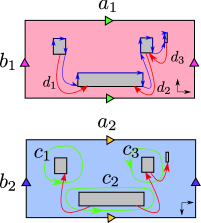
Figure 1. Basis for relative homology.

These paths form a basis of the relative homology group of $S$. According to Lemma 1 if we take the hat image of these homology elements besides from $\hat{\alpha}_{n-1}^{\prime}$ they form a basis of $H^{-}_{1}(\hat{S},\hat{\Sigma};\mathbb{C})$ which induce local coordinates in the stratum (see e.g. [AEZ16]) called period coordinates.

We also introduce $\beta^{\prime}_{i}$ for $1\leq i\leq n-1$ the last side of the rectangle that closes obstacle $i$. In other term, the class that satisfies $\alpha_{i}+\beta_{i}+\alpha^{\prime}_{i}+\beta^{\prime}_{i}=c_{i}$. For ways of intersection numbers with cylinders we will construct later, we will prefer to replace $c_{i}$ by $\beta^{\prime}_{i}$ in the basis and equations.

To write down equations in period coordinates we need to eliminate an ambiguity given by the non trivial holonomy of the surface. We choose a fundamental domain for the action of this holonomy given by the two copies glued along the vertical sides to which we remove the horizontal sides. This corresponds to drawing the copies reflected along the horizontal axis. Now the family $\mathcal{S}$ is defined locally by the following equations, where we make the abuse to write the homology class while meaning their period,

(1) $$\begin{split}&\mathrm{Im}(a_{1})=0\text{, }\mathrm{Re}(b_{1})=0\text{, }\mathrm{Re}(a_{1})=\mathrm{Im}(b_{1})\\ &\mathrm{Im}(\beta_{i})=0\text{, }\mathrm{Re}(\alpha_{i})=0\text{ for all }1\leq i\leq n\\ &d_{i}=\gamma_{i}-\overline{\gamma}_{i}\text{ for all }1\leq i\leq n-1\end{split}$$

(2) $$\begin{split}&a_{1}=a_{2}\text{, }b_{1}=-b_{2}\\ &\alpha_{i}=-\alpha_{i}^{\prime}\text{ for all }1\leq i\leq n-1\\ &\beta_{i}=-\beta_{i}^{\prime}\text{ for all }1\leq i\leq n-1\\ \end{split}$$

There are $2n+3$ real equations and $3n-1$ complex equations. The quadratic stratum is of complex dimension $6n$, thus the induced subspace is of real dimension $12n-2n-6n-1=4n-1$. On the other hand for the family of billiards, we have $2n$ variables for the size of each obstacle, $2n-2$ for relative position of the obstacles, and $1$ dimensions for the size of the square torus. Thus we have indeed listed all the equations that define our billiard family.

Below we show that these two sets of equations do not constrain the generic orbit closure for our billiards which as a consequence will be the whole stratum. The first argument relies on Lemma 4 and the second on Lemma 5.

First remark that the periods appearing in equations $(\ref{eq:first})$ are not constrained by equations $(\ref{eq:second})$. Lemma 4 then implies that the affine space corresponding to the orbit closure $L$ contains $\operatorname{Vect}_{\mathbb{C}}\left(a_{1},\beta_{i},d_{i},\gamma_{i}\right)$ and $\operatorname{Vect}_{\mathbb{C}}\left(b_{1},\alpha_{i},\gamma_{i}\right)$ and consequently does not satisfy neither of the equations in (1). We have shown that the orbit closure contains the space defined by equations (2).

In the following we demonstrate inductively that $L$ contains affine spaces defined by a smaller subset of equations in (2) which will eventually be empty. To do so we point out surfaces in the space defined by the given subset which have a cylinder rationally independent to any other ones in the same direction. We will show that all but one equations of this subset are respected by the shifted periods in Lemma 5. This will imply that the orbit closure contains the subspace defined by all but this latter equation.

We want to decorrelate the periods of $b_{1}$ and $b_{2}$ but in the family a cylinder in the torus along $a_{1}$ has always a symmetric counter-part along $a_{2}$. We use the fact proven above that in the orbit closure $\gamma_{i}$ and $d_{i}$ have no correlation thus we can move the obstacles in the two copies independently. Figure 2 shows how to have a cylinder in one torus and not in the other by moving the obstacles and obstructing the flow in one copy. For a generic choice of lengths, the hatched cylinder is not commensurable to any other cylinder and its core curve intersects only $b_{1}$. The cylinder deformation breaks the relation between $a_{1}$ and $a_{2}$ and the same construction in the vertical direction breaks the relation between $b_{1}$ and $b_{2}$. As a result, the affine space $L$ contains the space defined by equations (2) minus the equations on $a$ and $b$.

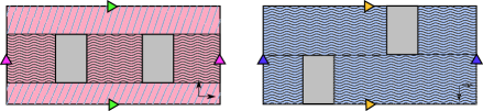
Figure 2. Good cylinder decomposition to deform $b_{1}$

Consider now the billiard with the same square obstacles of irrational side length such that all the obstacles are aligned in order. The distances between the obstacles are chosen such that they are rationally independent. On these surfaces there is a full decomposition in cylinders and all of the cylinders are rationally independent. The cylinder going from the right of the last obstacle to the left of the first intersects $b_{1},\alpha_{1}$ and $b_{2}$. The number of intersection of the core curve with each one of these curves is one. The previous argument has eliminated the constrains on $b_{1}$ and $b_{2}$ thus this cylinder deformation breaks the relation between $\alpha_{1}$ and $\alpha^{\prime}_{1}$.

Now by induction we take the cylinder intersecting $\alpha^{\prime}_{i}$ and $\alpha_{i+1}$. By assumption $\alpha^{\prime}_{i}$ does not appear in any equation and so we can break the relation between $\alpha_{i+1}$ and $\alpha^{\prime}_{i+1}$.

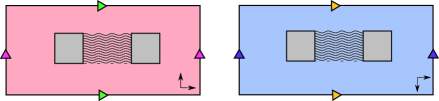
Figure 3. Good cylinder decomposition to deform $\alpha_{i}$

The same argument can be applied in the vertical direction for $\beta_{i}$ and $\beta^{\prime}_{i}$. This ends the proof of generic density for billiards in $\mathcal{S}(\mathcal{B}_{n})$.

This density result together with Lemma 3 and Corollary 1 imply the following,

Theorem 2.

The diffusion rate for Lebesgue-almost every windtree model in $B_{n}$ with $n\geq 2$ in Lebesgue-almost every direction is equal to the top Lyapunov exponent of $\mathcal{Q}(1^{4n})$.

4.2.2. Obstacles with many right angles.

Consider now a more general periodic windtree table with $n$ obstacles which are horizontal polygons with right angles. For each obstacle $i$ there are $k_{i}$ inward (concave) and $4+k_{i}$ outward (concave) right angles. Which implies that the obstacle has $2+k_{i}$ vertical and $2+k_{i}$ horizontal sides. We denote this family by $\mathcal{B}_{n}(k_{1},\dots,k_{n})$.

The associated quadratic differential has simple zeros at the outward right angles and poles at the inward. It has genus $n+1$ and is in the stratum

$$\mathcal{Q}(1^{4n+p},-1^{p})$$

where $p=\sum k_{i}$.

To construct a basis of homology of the associated translation surface, we start from the left point of the lowest horizontal side and browse the obstacle boundary clockwise until we come back to the starting point. This yields saddle connections $\alpha^{1}_{i},\beta^{1}_{i},\alpha^{2}_{i},\dots,\alpha^{4+k_{i}}_{i},\beta^{4+k_{i}}_{i}$. The classes $\alpha^{4+k_{n}}_{n}$ and $\beta^{4+k_{n}}_{n}$ are not taken into consideration to yield a basis of $H^{-}_{1}(S,\Sigma;\mathbb{C})$. Let $\gamma_{i}$ be the path joining the starting points two consecutive obstacles $i$ and $i+1$ and define as in the previous section absolute homology classes $a,b$ and $d$.

The equations in period coordinates are very similar as in the previous case, we only need to adapt equations on the obstacles.

$$\begin{split}&\mathrm{Im}(a_{1})=0\text{, }\mathrm{Re}(b_{1})=0\text{, }\mathrm{Re}(a_{1})=\mathrm{Im}(b_{1})\\ &\mathrm{Re}(\alpha^{j}_{i})=0\text{ for all }1\leq i\leq n\text{ and }1\leq j\leq 2+k_{i}-1\\ &\mathrm{Im}(\beta^{j}_{i})=0\text{ for all }1\leq i\leq n\text{ and }1\leq j\leq 2+k_{i}-1\\ &d_{i}=\gamma_{i}-\overline{\gamma}_{i}\text{ for all }1\leq i\leq n-1\end{split}$$

$$\begin{split}&a_{1}=a_{2}\text{, }b_{1}=-b_{2}\\ &\sum_{j=1}^{4+k_{i}}\alpha^{j}_{i}=0\text{ for all }1\leq i\leq n-1\\ &\sum_{j=1}^{4+k_{i}}\beta^{j}_{i}=0\text{ for all }1\leq i\leq n-1\\ \end{split}$$

There are now $\sum(4+2k_{i}-2)+3=2n+2p+3$ real equations and $3n-1$ complex equations. The quadratic stratum is of complex dimension

$$2(n+1)+4n+2p-2=6n+2p$$

thus the induced subspace is of real dimension

$$12n+4p-2n-2p-3-6n+2=4n+2p-1.$$

On the other hand for the family of billiards, we have $\sum(4+2k_{i}-2)=2n+2p$ variables for the size of each obstacle, $2n-2$ for relative position of the obstacles, and $1$ dimensions for the size of the square torus. Thus we have indeed listed all the equations that define our billiard family.

The first part of the previous argument applies verbatim to this case with the real and imaginary part equations. For the second part we need to exhibit a similar construction of cylinders. The construction of Figure 2 is straightforward to generalise to any shape of obstacle. We will detail the generalisation of the construction in Figure 3.

Start with the vertical side that does not appear in the basis. Now we can find an element of the family such that the obstacle $n$ is in the neighborhood of a rectangle as in Figure 4, making every other side very small, and similarly for the first obstacle. There is a horizontal cylinder joining the given side of obstacle $n$ with a side of the first obstacle. This surface will be completely decomposed into horizontal cylinders and the lengths are chosen to be all rationally independent.

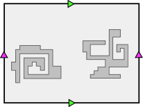
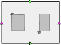
Figure 4. Example of deformation

This enables us to break the equation constraining the $\alpha_{1}^{j}$. Then by induction we show that a generic billiard in $\mathcal{B}_{n}(k_{1},\dots,k_{n})$ induces a quadratic differentials with dense orbits in the stratum. We have the following theorem,

Theorem 3.

For any $n\geq 2$, $k_{1},\dots k_{n}\geq 0$ and $p=\sum k_{i}$, the diffusion rate for in Lebesgue-almost every windtree model $B_{n}(k_{1},\dots,k_{n})$ in Lebesgue-almost every direction is equal to the top Lyapunov exponent of $\mathcal{Q}(1^{4n+p},-1^{p})$.

5. Some numerical computations

Figure 5 shows numerical approximations of the principal Lyapunov exponent of strata $\mathcal{Q}(1^{4n})$. We observe that it goes to $1/2$ when $n\to\infty$.

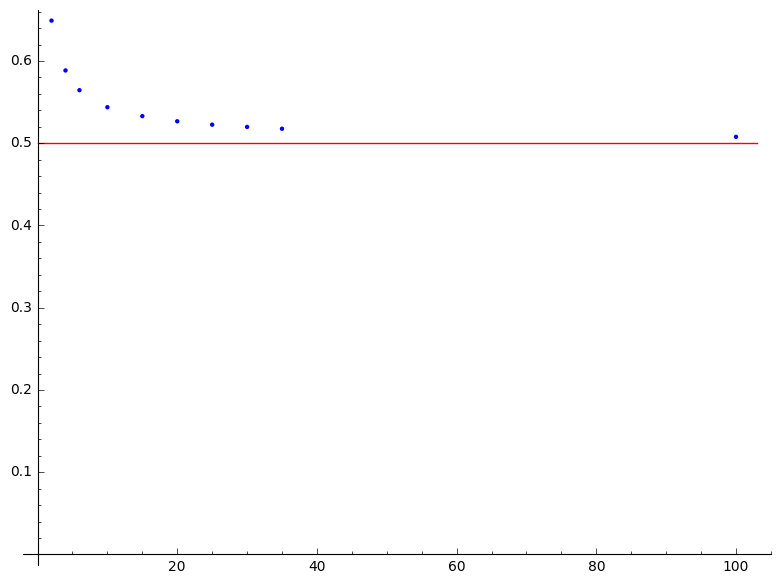
Figure 5. Principal Lyapunov exponent for $\mathcal{Q}(1^{4n})$

In Figure 6, we represent a computation of the principal Lyapunov exponent for $\mathcal{Q}(1^{4n+10},-1^{10})$. When we fix the number of simple poles and increase the number of simple zeros, the diffusion rate again goes to $1/2$ but now by smaller values.

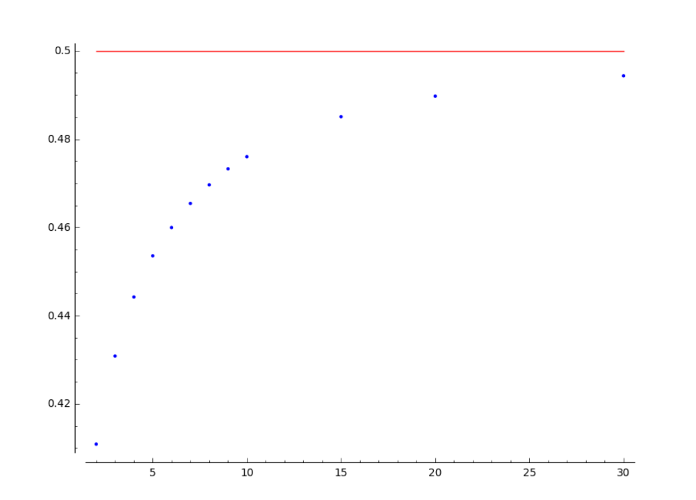
Figure 6. Principal Lyapunov exponent for $\mathcal{Q}(1^{4n+10},-1^{10})$

The $1/2$ value is also the diffusion rate for the Brownian motion. Intuitively, these convex angles scatter the linear flow which follows completely different paths from one side to the other of the singularity. They mimic the hyperbolic behaviour of smooth convex obstacles.

An opposite behaviour is given by the concave right angles of the obstacles. In Figure 7, we present the largest Lyapunov exponent of strata corresponding to windtrees with two obstacles with an increasing number of concave angles.

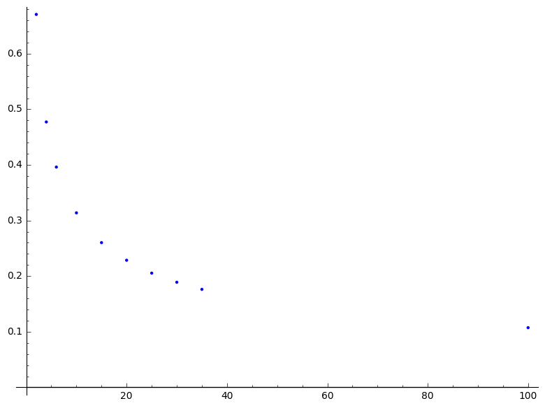
Figure 7. Principal Lyapunov exponent for $\mathcal{Q}(1^{8+p},-1^{p})$

Further experiments show that in contrary to the previous case for a fixed number of simple zeros and a number of simple poles going to infinity, the principal Lyapunov exponent is going to zero. A heuristic explanation for this phenomenon is that when the flow hits the obstacle close to a concave right angle in the billiard it comes back on its steps slightly shifted as drawn in Figure 8. This enters in resonance with the result of [DZ15] which states that when we increase the number of concave right angles of a single obstacle for a periodic windtree, the diffusion rate goes to zero. This also enters in the frame of the more general Grivaux-Hubert conjecture that we explore and reformulate in [Fou16].

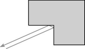
Figure 8. Flow bouncing close to a concave right angle.

Appendix A Generic Lyapunov exponent

In this section we follow the proof of [CE15] which shows that any translation surface is Lyapunov and Birkhoff generic in its orbit closure for almost every direction. We will focus on one of the key results in this article about Lyapunov genericity on a irreducible component for the Kontsevich-Zorich cocycle.

Theorem (1.5 in [CE15]).

Fix $x\in\mathcal{H}_{1}(\alpha)$ and let $\mathcal{M}=\overline{\mathrm{SL}(2,\mathbb{R})x}$ the smallest affine invariant manifold containing $x$, let $V$ be a $\mathrm{SL}(2,\mathbb{R})$ invariant subbundle of the Hodge bundle which is defined and continuous on $\mathcal{M}$. Let $A_{V}:\mathrm{SL}(2,\mathbb{R})\times\mathcal{M}\rightarrow V$ denote the restriction of the Kontsevich-Zorich cocycle to $V$ and suppose that $A_{V}$ is strongly irreducible with respect to the affine measure $\nu_{\mathcal{M}}$ whose support is $\mathcal{M}$. Then, for almost every $\theta\in[0,2\pi)$,

$$\lim_{t\to\infty}\frac{\log||A_{V}(g_{t}r_{\theta}x)||}{\log t}\to\lambda_{1}$$

where $\lambda_{1}$ is the top Lyapunov exponent of $A_{V}$.

Our purpose here is to show the following additional lemma to this theorem, introduced as Lemma 1 in section 3.

Lemma.

In the previous theorem, for any $h\in V$ and almost every $\theta\in[0,2\pi)$

$$\lim_{t\to\infty}\frac{\log||A_{V}(g_{t}r_{\theta}x)h||}{\log t}\to\lambda_{1}.$$

In [CE15] intuition of the result is provided by analogy with random walks. We start by showing the analog of Lemma 1 for random walks.

A.1. Random walks

Let $\mu$ be a $\mathrm{SO}(2,\mathbb{R})$-invariant compactly supported measure on $\mathrm{SL}(2,\mathbb{R})$ which is absolutely continuous with respect to Haar measure. A measure $\nu$ on $\mathcal{H}_{1}(\alpha)$ is called $\mu$-stationary if

$$\mu*\nu=\int_{\mathrm{SL}(2,\mathbb{R})}(g_{*}\nu)d\mu(g)=\nu.$$

By a theorem of Furstenberg [Fur63b], [Fur63a], restated in [NZ99][Theorem 1.4], there exists a probability measure $\rho$ on $\mathrm{SL}(2,\mathbb{R})$ such that the map $\nu\to\rho*\nu$ is a bijection between ergodic measures for the action of upper triangular subgroup of $\mathrm{SL}(2,\mathbb{R})$ and ergodic $\mu$ stationary measures which are $\mathrm{SL}(2,\mathbb{R})$-invariant affine measures according to [EM13][Theorem 1.4].
This is a first step for an analogy between Teichmüller flow in some affine invariant locus and a random walk with the associated measure.

Let $\mathrm{Gr}_{s}$ denote the grassmanian of $s$-dimensional subspaces in the $\mathrm{SL}(2,\mathbb{R})$ invariant subbundle of the Hodge bundle $V$. Let $\tilde{\mathcal{H}}=\mathcal{H}_{1}(\alpha)\times\mathrm{Gr}_{s}$ and $\tilde{\nu}$ be the $\mu$ stationary measure on it; we may write $d\tilde{\nu}(x,U)=d\nu(x)d\eta_{x}(U)$.

The measure $\eta_{x}$ on $\mathrm{Gr}_{s}$ heuristically corresponds to the mean position of any linear subspace carried along the Teichmüller flow using Gauss-Manin connection. Let $h$ be some vector in $V\setminus 0$ and $I(h)\subset\mathrm{Gr}_{s}$ be the set of $s$-dimensional subspaces containing $h$.

Lemma (C.10 in [EM13]).

If the cocycle $A_{V}$ is strongly irreducible on $V$ then for almost every $x\in\mathcal{H}_{1}(\alpha)$ and any vector $h_{x}\in V$, $\delta_{x}(I(h_{x}))=0$

In particular if we consider some Oseledets flag this Lemma yields that generically they do not contain a fixed vector $h$ along random walks.

We show a random walk version of the theorem in the previous paragraph,

Theorem 4 (Theorem 2.6 and Lemma 2.9 of [CE15]).

Fix $x\in\mathcal{H}_{1}(\alpha)$ and let $\mathcal{M}=\overline{\mathrm{SL}(2,\mathbb{R})\cdot x}$ the smallest affine invariant manifold containing $x$, let $V$ be a $\mathrm{SL}(2,\mathbb{R})$ invariant subbundle of the Hodge bundle which is defined and continuous on $\mathcal{M}$. Let $A_{V}:\mathrm{SL}(2,\mathbb{R})\times\mathcal{M}\rightarrow V$ denote the restriction of the Kontsevich-Zorich cocycle to $V$ and suppose that $A_{V}$ is strongly irreducible with respect to the affine measure $\nu_{\mathcal{M}}$ whose support is $\mathcal{M}$. Then for a fixed $h\in V$ and for $\mu^{\mathbb{N}}$-almost every $\overline{g}=(g_{1},\dots,g_{n},\dots)$,

$$\lim_{n\to\infty}\frac{1}{n}\log||A_{V}(g_{n}\dots g_{1},x)h||\to\lambda_{1}$$

where $\lambda_{1}$ is the top Lyapunov exponent of $A_{V}$.

This theorem already appears in [CE15] as a remark to a more general theorem. We reformulate the proof in this specific case for convenience to the reader.

A.2. Proof Theorem 4

We fix $\mathcal{M}$ and $V$ as in the theorem. Pick an arbitrary $v_{0}\in V$ and let $v_{i}(\overline{g})=A_{V}(g_{i}\dots g_{1},x)v_{0}$. The key tool to show this theorem is a decomposition lemma for the sequences of cocycle in the case of strong irreducibility.

Lemma (2.11 and 2.16 in [CE15]).

For all $\epsilon>0$, there exists an integer $L$ such that for every $x\in\mathcal{M}$ almost every $\overline{g}$ we have that all but a set of $\mathbb{N}$ of density $4\epsilon$ is in disjoint blocks $[i+1,i+L]$ so that

$$\exp(\lambda_{1}-\epsilon)^{L}\leq\frac{||A_{v}(g_{i+L}\dots g_{i+1},y)v||}{||v||}\leq\exp(\lambda_{1}+\epsilon)^{L}.$$

Proof.

Refer to section 2.3 of [CE15].
∎

Now let $\overline{g}$ be in the full measure set as above, $K$ be the subset of density $4\epsilon$ and $I$ the set of indices $i$ in the blocks $[i+1,i+L]$. Then for $n\gg L$,

$$\log||v_{n}|| =\sum_{i=1}^{n}\log\frac{||v_{i}||}{||v_{i-1}||}$$

$$=\underbrace{\sum_{i\in I\cap[1,n-L]}\log\frac{||v_{i+L}||}{||v_{i}||}}_{S_{1}}+\underbrace{\sum_{i\in K\cap[1,n-L]}\log\frac{||v_{i}||}{||v_{i-1}||}}_{S_{2}}+\underbrace{\sum_{i=n-L^{\prime}+1}^{n}\log\frac{||v_{i}||}{||v_{i-1}||}}_{S_{3}}$$

where $n-L^{\prime}=\max\{n-L,I+L\}$.

Let $C$ such that for all $g$ in the support of $\mu$ and all $y\in\mathcal{M}$, $||A_{V}(g,y)||\leq C$. Then $|S_{3}|\leq L\log C$, and $|S_{2}|\leq 4\epsilon n\log C$.
Moreover

$$\frac{|I\cap[1,\dots,n]|\cdot L}{n}\geq 1-4\epsilon$$

Hence

$$S_{1}\geq\left|I\cap[1,\dots,n]\right|\cdot(\lambda_{1}-\epsilon)L\geq(1-4\epsilon)n(\lambda_{1}-\epsilon)$$

and

$$\frac{1}{n}\log||v_{n}||\geq(1-4\epsilon)(\lambda_{1}-\epsilon)-4\epsilon\log C-\frac{L}{n}\log C$$

for almost every $\overline{g}$ and any $n\gg L$.

Since $\epsilon\geq 0$ is arbitrary, we get for all $h\in V$ and almost every $\overline{g}$,

$$\liminf_{n\to\infty}\log||A_{V}(g_{n}\dots g_{1},x)h||\geq\lambda_{1}.$$

And with a similar argument we get an upper bound

$$\limsup_{n\to\infty}\log||A_{V}(g_{n}\dots g_{1},x)h||\leq\lambda_{1}.$$

Which implies Theorem 4.

A.3. Proof of Lemma 1

According to the sublinear tracking Lemma of [CE15], for almost every $\theta\in[0,2\pi)$, there exists $\overline{g}=(g_{1},\dots,g_{n},\dots)$ satisfying Theorem 4 such that we can write

$$g_{\lambda n}r_{\theta}=\epsilon_{n}g_{n}\dots g_{1}$$

with $\epsilon_{n}\in\mathrm{SL}(2,\mathbb{R})$ satisfying

$$\lim_{n\to\infty}\frac{1}{n}\log||\epsilon_{n}||=0$$

By the cocycle relation we have

$$A_{V}(g_{\lambda n},r_{\theta}x)=A_{V}(\epsilon_{n},g_{n}\dots g_{1}x)A_{V}(g_{n}\dots g_{1},x).$$

But there exists $C>0$ and $N<\infty$ so that for all $g\in\mathrm{SL}(2,\mathbb{R})$ and all $x\in\mathcal{H}_{1}(\alpha)$,

$$||A_{V}(g,x)||\leq C||g||^{N}.$$

Hence

$$\log||A_{V}(g_{\lambda n},r_{\theta}x)h||=\log||A_{V}(g_{n}\dots g_{1},x)||h+o(n).$$

Which shows the Lemma.

References

- [AEZ16] Jayadev S. Athreya, Alex Eskin, and Anton Zorich. Right-angled billiards and volumes of moduli spaces of quadratic differentials on . Ann. Sci. Éc. Norm. Supér., 49(6), 2016.
- [BS81] L. A. Bunimovich and Ya. G. Sinaĭ. Markov partitions for dispersed billiards. Comm. Math. Phys., 78(2):247–280, 1980/81.
- [CE15] Jon Chaika and Alex Eskin. Every flat surface is Birkhoff and Oseledets generic in almost every direction. J. Mod. Dyn., 9:1–23, 2015.
- [D+16] Vincent Delecroix et al. surface_dynamics, 2016.
- [DHL14] Vincent Delecroix, Pascal Hubert, and Samuel Lelièvre. Diffusion for the periodic wind-tree model. Ann. Sci. Éc. Norm. Supér. (4), 47(6):1085–1110, 2014.
- [DZ15] Vincent Delecroix and Anton Zorich. Cries and whispers in wind-tree forests, 2015.
- [EE90] Paul Ehrenfest and Tatiana Ehrenfest. The conceptual foundations of the statistical approach in mechanics. Dover Publications, Inc., New York, english edition, 1990. Translated from the German by Michael J. Moravcsik, With a foreword by M. Kac and G. E. Uhlenbeck.
- [EFW18] Alex Eskin, Simion Filip, and Alex Wright. The algebraic hull of the Kontsevich–Zorich cocycle. Ann. of Math. (2), 188:281–313, 2018.
- [EM13] Alex Eskin and Maryam Mirzakhani. Invariant and stationary measures for the sl(2,r) action on moduli space, 2013.
- [EMM15] Alex Eskin, Maryam Mirzakhani, and Amir Mohammadi. Isolation, equidistribution, and orbit closures for the action on moduli space. Ann. of Math. (2), 182(2):673–721, 2015.
- [Fou16] Charles Fougeron. Lyapunov exponents of the hodge bundle over strata of quadratic differentials with large number of poles, 2016.
- [FU14] Krzysztof Fraczek and Corinna Ulcigrai. Non-ergodic -periodic billiards and infinite translation surfaces. Invent. Math., 197(2):241–298, 2014.
- [Fur63a] Harry Furstenberg. Noncommuting random products. Trans. Amer. Math. Soc., 108:377–428, 1963.
- [Fur63b] Harry Furstenberg. A Poisson formula for semi-simple Lie groups. Ann. of Math. (2), 77:335–386, 1963.
- [GR17] R. Gutiérrez-Romo. Simplicity of the lyapunov spectra of certain quadratic differentials, 2017.
- [HW80] J. Hardy and J. Weber. Diffusion in a periodic wind-tree model. J. Math. Phys., 21(7):1802–1808, 1980.
- [MST18] Alba Málaga Sabogal and Serge Eugene Troubetzkoy. Infinite Ergodic Index of the Ehrenfest Wind-Tree Model. Comm. Math. Phys., 358(3):995–1006, 2018.
- [NZ99] Amos Nevo and Robert J. Zimmer. Homogenous projective factors for actions of semi-simple Lie groups. Invent. Math., 138(2):229–252, 1999.
- [SV04] Domokos Szász and Tamás Varjú. Markov towers and stochastic properties of billiards. In Modern dynamical systems and applications, pages 433–445. Cambridge Univ. Press, Cambridge, 2004.
- [Vee93] William A. Veech. Flat surfaces. Amer. J. Math., 115(3):589–689, 1993.
- [Wri14] Alex Wright. The field of definition of affine invariant submanifolds of the moduli space of abelian differentials. Geom. Topol., 18(3):1323–1341, 2014.
- [Wri15] Alex Wright. Cylinder deformations in orbit closures of translation surfaces. Geom. Topol., 19(1):413–438, 2015.