Darling–Kac theorem for renewal shifts
in the absence of regular variation

Abstract

We study null recurrent renewal Markov chains with renewal distribution in the domain of geometric partial attraction of a semistable law. Using the classical procedure of inversion, we derive a limit theorem similar to the Darling–Kac law along subsequences and obtain some interesting properties of the limit distribution. Also in this context, we obtain a Karamata type theorem along subsequences for positive operators. In both results, we identify the allowed class of subsequences. We provide several examples of nontrivial infinite measure preserving systems to which these results apply.

1 Introduction and summary of main results

We recall that regular variation is an essential condition for the existence of a Darling–Kac law [12]. Restricting to the simple setting of one-sided null recurrent renewal chains, our aim is to understand what happens if the regular variation is replaced by a weaker assumption on the involved ‘renewal’ distribution. As we explain in the sequel, we will assume that this distribution is in the domain of geometric partial attraction of a semistable law, a subclass of infinitely divisible laws. Among the main references for ground results on semistable laws, we recall that the behaviour of the associated characteristic function has been first understood by Kruglov [26] and that a probabilistic approach in understanding such laws has been developed by Csörgő [9]. For more recent advances on ‘merging results’ we refer to Csörgő and Megyesi [10], Kevei [22], and references therein.

The classical Darling–Kac law for one-sided null recurrent renewal shifts / Markov chains is recalled in Subsection 1.1. The analogue of this law in the semistable setting is contained in Section 3; this is the content of Theorem 3.1. Several properties of the limit distribution appearing in Theorem 3.1 are discussed in Section 4. In particular, we study the asymptotic behaviour of this distribution at $0$ and $\infty$. Although, as recalled in Section 4, the asymptotic behaviour at $\infty$ can be read off from previous results, we note the somewhat surprising result Theorem 4.5 that gives the asymptotic behaviour of this distribution at $0$. In Section 5 we determine the asymptotics of the renewal function in the semistable setup, and extend this result for positive operators. In Section 6 we provide a number of examples (notably, perturbed Wang maps and piecewise linear Fibonacci maps) to which Theorem 3.1 applies. The examples considered in Section 6 are dynamical systems that are isomorphic to Markov chains. In Section 7, we discuss the application of Theorem 3.1 to specific dynamical systems that are not isomorphic to a Markov chain. Finally, some technical proofs are contained in the Appendix.

1.1 Darling–Kac law for null recurrent renewal chains under regular variation

Fix a probability distribution $(f_{k})_{k\geq 0}$, $\sum_{k=0}^{\infty}f_{k}=1$, and consider the Markov renewal chain $(X_{n})_{n\geq 0}$, $X_{n}\in{\mathbb{N}}_{0}={\mathbb{N}}\cup\{0\}$ with transition probabilities

$$p_{\ell,k}:={\mathbb{P}}(X_{n+1}=k|X_{n}=\ell)=\begin{cases}f_{k},&\ell=0,\\ 1,&k=\ell-1,\ \ell\geq 1,\\ 0,&\text{otherwise.}\end{cases}$$ (1.1)

Clearly, $X_{n}$ is a recurrent Markov chain, with unique invariant measure

$$\pi_{n}=\pi_{0}\sum_{i=n}^{\infty}f_{i},\quad n\geq 1,\quad\text{and }\,\pi_{0}>0.$$ (1.2)

The chain is null recurrent (i.e. the invariant measure is infinite) if and only if $\sum_{k=1}^{\infty}kf_{k}=\infty$, which we assume in the following.

Assume that the chain starts from 0, i.e. $X_{0}=0$, and let $0=Z_{0}<Z_{1}<Z_{2}<\ldots$ denote the consecutive return times to 0. Since the Markov chain is recurrent, all these random variables are a.s. finite, and by the Markov property

$$Z_{n}=\tau_{1}+\tau_{2}+\ldots+\tau_{n},\quad n\geq 1,$$

where $\tau,\tau_{1},\tau_{2},\ldots$ are iid random variables, with distribution ${\mathbb{P}}(\tau=k)=f_{k-1}$, $k\geq 1$.

Let

$$S_{n}=\sum_{j=0}^{n-1}1_{X_{j}=0},\quad n\geq 1,$$

denote the occupation time of $0$, i.e. the number of visits to $0$ up to time $n-1$. Recall the duality rule between $S_{n}$ and $Z_{m}$

$$S_{n}\geq m\ \,\Longleftrightarrow\ Z_{m-1}\leq n-1,$$ (1.3)

which means that the number of visits to the state $0$ before time $n$ is at least $m$ if and only if the $(m-1)$st return takes place before time $n$.

Up to now everything holds true for a general recurrent Markov renewal chain. In what follows, we recall how a distributional limit theorem for $Z_{n}$ translates to a limit theorem for $S_{n}$. To do so, we assume that $(f_{j})_{j\geq 0}$ is in the domain of attraction of an $\alpha$-stable, $\alpha<1$; that is,

$$\sum_{j\geq n}f_{j}=\ell(n)n^{-\alpha},$$

for a slowly varying function $\ell$. Then

$$\frac{Z_{n}}{n^{1/\alpha}\ell_{1}(n)}\rightarrow^{d}Z_{\alpha},$$ (1.4)

with the norming sequence $n^{1/\alpha}\ell_{1}(n)$ being the asymptotic inverse of $n^{\alpha}/\ell(n)$, where $Z_{\alpha}$ is an $\alpha$-stable law and $\to^{d}$ stands for convergence in distribution. In the following all nonspecified limit relations are meant as $n\to\infty$. It is known (see, for instance, Bingham [3]) that the stable limit law for $Z_{n}$ can be translated into a Darling–Kac law for $S_{n}$.

Let $\mathcal{M}_{\alpha}$ be a positive random variable distributed according to the normalised Mittag-Leffler distribution of order $\alpha$, that is $\mathbb{E}(e^{z\mathcal{M}_{\alpha}})=\sum_{p=0}^{\infty}\Gamma(1+\alpha)^{p}z^{p}/\Gamma(1+p\alpha)$ for all $z\in{\mathbb{C}}$. We recall that ${\mathcal{M}}_{\alpha}=^{d}(Z_{\alpha})^{-\alpha}$ and sketch the argument for obtaining a Darling–Kac law from (1.3) and (1.4).

Let $b(n)=n^{1/\alpha}\ell_{1}(n)$ and let $a(n)=n^{\alpha}/\ell(n)$ be its asymptotic inverse, that is $a(b(n))\sim n$. In what follows, to ease notation we suppress the integer part. Using (1.3), and $b(a(n)x)\sim x^{1/\alpha}n$, $n\to\infty$, we obtain

$$\begin{split}{\mathbb{P}}(S_{n}\geq a(n)x)&={\mathbb{P}}(Z_{a(n)x-1}\leq n-1)\\ &={\mathbb{P}}\Big{(}\frac{Z_{a(n)x-1}}{b(a(n)x-1)}\leq\frac{n-1}{b(a(n)x-1)}\Big{)}\\ &\rightarrow{\mathbb{P}}(Z_{\alpha}\leq x^{-1/\alpha})\\ &={\mathbb{P}}({\mathcal{M}}_{\alpha}\geq x).\end{split}$$

Hence, $S_{n}/a(n)\to^{d}{\mathcal{M}}_{\alpha}$, which gives the Darling–Kac law in this simplified setting.

As already mentioned, in what follows we employ the inversion procedure described above weakening the assumption on $\tau$. Namely, we will assume that $\tau$ is in the domain of geometric partial attraction of a semistable law of order $\alpha\in(0,1)$, as recalled in Section 2.

1.2 Renewal chain, induced renewal chain

Put $X={\mathbb{N}}_{0}^{{\mathbb{N}}_{0}}$ and let $T:X\to X$ be the shift map. Introduce the cylinders

$$[e_{0}e_{1}\ldots e_{k-1}]:=\{x=(x_{0},x_{1},\ldots)\in X\,:\,x_{i}=e_{i},\ i=0,1,\ldots,k-1\}.$$

We define the $T$-invariant measure $\mu$ as

$$\mu([e_{0}e_{1}\ldots e_{k-1}])=\mu([e_{0}])p_{e_{0}e_{1}}\cdots p_{e_{k-2}e_{k-1}},$$

where $\mu([j])=\pi_{j}$ given in (1.2). The measure extends uniquely to the $\sigma$-algebra generated by the cylinder sets. For simplicity, we assume that $\mu([0])=\pi_{0}=1$.

Let $Y=[0]=\{x\in X:x_{0}=0\}$, and decompose

$$Y=\cup_{k\geq 0}C_{k},\quad\text{ where }C_{k}=[0,k,k-1,k-2,\dots,0].$$

The cylinders $C_{k}$ are pairwise disjoint, and their measures are given by

$$\mu(C_{k})=\mu(Y)p_{0,k}p_{k,k-1}\cdots p_{1,0}=f_{k}.$$

We recall the definition of the induced shift on $Y$ and associated ‘induced renewal chain’. For $y\in Y$, let $\tau(y)=\min\{n\geq 1:T^{n}(y)\in Y\}$ and $T_{Y}=T^{\tau}$. The probability measure $\nu=\mu(Y)^{-1}\mu|_{Y}=\mu|_{Y}$ is $T_{Y}$-invariant. To see this it is enough to show that $\nu(C_{k})=\nu(T_{Y}^{-1}C_{k})$ for any $k\geq 0$. Noting that

$$T_{Y}^{-1}(C_{k})=\cup_{\ell=0}^{\infty}[0,\ell,\ell-1,\ldots,1,0,k,k-1,\ldots,1,0]$$

we have

$$\begin{split}\nu(T_{Y}^{-1}C_{k})&=\sum_{\ell=0}^{\infty}\nu([0,\ell,\ell-1,\ldots,1,0,k,k-1,\ldots,1,0])\\ &=\sum_{\ell=0}^{\infty}\frac{\mu([0])f_{\ell}f_{k}}{\mu([0])}\\ &=f_{k}=\nu(C_{k}).\end{split}$$

We note that $C_{k}=\{y\in Y:\tau(y)=k+1\}$ and that $T_{Y}$ can be regarded as the shift on the space $(\{C_{k}\}_{k\geq 0})^{{\mathbb{N}}_{0}}$. Given that ${\mathcal{B}}_{Y}$ is the $\sigma$-algebra generated by cylinders, the induced shift $(Y,{\mathcal{B}}_{Y},T_{Y},\nu)$ is a probability measure preserving transformation.

1.3 Renewal sequences and transfer operators associated with Markov shifts

In the set-up of Subsection 1.2, we recall that the renewal sequence $\{u_{n}\}_{n\geq 1}$ associated with the recurrent shift $(X,{\mathcal{B}}_{X},T,\mu)$ is given by

$$u_{0}=1,\quad u_{n}=\sum_{j=1}^{n}f_{j}u_{n-j}.$$

We let $L:L^{1}(\mu)\to L^{1}(\mu)$ be the transfer operator associated with the shift $(X,{\mathcal{B}}_{X},T,\mu)$ defined by $\int_{X}L^{n}v\cdot w\,\mathrm{d}\mu=\int_{X}v\cdot w\!\circ\!T^{n}\,\mathrm{d}\mu$, $n\geq 1$, $v\in L^{1}(\mu)$, $w\in L^{\infty}(\mu)$. Roughly, the operator $L$ describes the evolution of (probability) densities under the action of $T$. Alternatively, the operator $L$ acting on piecewise constant functions (that is, constant functions on cylinder sets) can be identified with the stochastic matrix with entries $p_{\ell,k}$ given in (1.1). Moreover, the following holds a.e. on $Y=[0]$ (for a precise reference, see, for instance, Aaronson [1, Proposition 5.1.2 and p. 157]),

$$p_{0,0}^{(n)}=L^{n}1_{[0]}=L^{n}(1_{Y})=u_{n}=\mu(Y\cap T^{-n}Y),$$ (1.5)

and the equality $L^{n}1_{[s]}=\mu([s]\cap T^{-n}[s])$ hold a.e. on any cylinder $[s]$. Under the assumption that the tail sequence $\mu(\tau>n)$ is regularly varying with some index in $[0,1]$, the asymptotic behaviour of the partial sum $\sum_{j=0}^{n-1}u_{j}=\sum_{j=0}^{n-1}L^{j}1_{Y}$, is well understood; for results in terms of renewal sequences see, for instance, Bingham et al.[5, Section 8.6.2]; for results stated in terms of both average transfer operators and renewal sequences we refer to [1, Chapter 5].

The asymptotic behaviour of the partial sum $\sum_{j=0}^{n-1}L^{j}1_{Y}$ has also been understood for several classes of infinite measure preserving systems $(X,{\mathcal{B}}_{X},T,\mu)$ that are not isomorphic to renewal shifts. Provided the existence of a suitable reference set $Y\subset X$, one considers the return time $\tau$ to $Y$ and obtains a finite measure preserving system $(Y,{\mathcal{B}}_{Y},T^{\tau},\mu_{Y})$. In case $\mu_{Y}(\tau>n)$ is regularly varying with index $\alpha<1$, under certain assumptions on $(Y,{\mathcal{B}}_{Y},T^{\tau},\mu_{Y})$, it has been shown that for $a_{n}=C\mu_{Y}(\tau>n)(1+o(1))$, with $C>0$ (depending on the parameters of the map $T$), $a_{n}^{-1}\sum_{j=0}^{n-1}L^{j}v$ convergences uniformly on suitable compact subsets of $X$ and suitable observable $v$. For a precise statement we refer to the work of Thaler [36]; for more recent results see Thaler and Zweimüller [37], Melbourne and Terhesiu [30], and references therein.

In the present work we assume that $\tau$ is in the domain of geometric partial attraction of a semistable law of order $\alpha\in(0,1)$ (as in Section 2). The task is to obtain a Karamata type theorem along subsequences, identifying the allowed class of subsequences. For renewal shifts (and implicitly, infinite measure preserving systems that come equipped with an iid sequence $(\tau\!\circ\!T_{Y}^{n})$), this type of result was obtained by Kevei [23] and in Section 5 we recall this result. The new result in this context is Theorem 5.2, which gives a Karamata type theorem along subsequences for positive operators. In Section 7, we discuss its application to infinite measure preserving specific systems not isomorphic to renewal shifts; in particular we obtain uniform convergence of the partial sum of transfer operators along subsequences on suitable sets.

2 Semistable laws

The class of semistable laws, introduced by Paul Lévy in 1937, is an important subclass of infinitely divisible laws. For definitions, properties, and history of semistable laws we refer to Sato [34, Chapter 13], Meerschaert and Scheffler [27], Megyesi [28], Csörgő and Megyesi [10], and the references therein. Here we summarise the main results from [28, 10], and we specialise these results to nonnegative semistable laws.

2.1 Definition and some properties

Semistable laws are limits of centred and normed sums of iid random variables along subsequences $k_{n}$ for which

$$k_{n}<k_{n+1}\ \text{for }n\geq 1\ \text{and }\lim_{n\to\infty}\frac{k_{n+1}}{k_{n}}=c>1$$ (2.1)

hold. Since $c=1$ corresponds to the stable case ([28, Theorem 2]), we assume that $c>1$. The simplest such a sequence is

$$k_{n}=\lfloor c^{n}\rfloor,$$

where $\lfloor\cdot\rfloor$ stands for the (lower) integer part. In what follows we let $c$ be as defined in (2.1).

The characteristic function of a nonnegative semistable random variable $V$ has the form

$$\mathbb{E}e^{\mathfrak{i}tV}=\exp\left\{\mathfrak{i}ta+\int_{0}^{\infty}(e^{\mathfrak{i}tx}-1)\mathrm{d}R(x)\right\},$$

where $a\geq 0$, and $M:(0,\infty)\to(0,\infty)$ is a logarithmically periodic function with period $c^{1/\alpha}>1$, i.e. $M(c^{1/\alpha}x)=M(x)$ for all $x>0$, such that $-R(x):=M(x)/x^{\alpha}$ is nonincreasing for $x>0$, $\alpha\in(0,1)$. We further assume that $V$ is nonstable, that is $M$ is not constant.

2.2 Domain of geometric partial attraction

In the following $X,X_{1},X_{2},\ldots$ are iid random variables with distribution function $F(x)={\mathbb{P}}(X\leq x)$. We fix a semistable random variable $V=V(R)$ with characteristic and distribution function

$$\mathbb{E}e^{\mathfrak{i}tV}=\exp\left\{\int_{0}^{\infty}(e^{\mathfrak{i}tx}-1)\mathrm{d}R(x)\right\},\quad G(x)={\mathbb{P}}(V\leq x).$$ (2.2)

The random variable $X$ belongs to the domain of geometric partial attraction of the semistable law $G$ if there is a subsequence $k_{n}$ for which (2.1) holds, and a norming and a centring sequence $A_{n},B_{n}$, such that

$$\frac{\sum_{i=1}^{k_{n}}X_{i}}{A_{k_{n}}}-B_{k_{n}}\rightarrow^{d}V.$$ (2.3)

It turns out that without loss of generality we may assume that

$$A_{n}=n^{1/\alpha}\ell_{1}(n)$$

with some slowly varying function $\ell_{1}$ (see [28, Theorem 3]). In order to characterise the domain of geometric partial attraction we need some further definitions. As $k_{n+1}/k_{n}\to c>1$, for any $x$ large enough there is a unique $k_{n}$ such that $A_{k_{n}}\leq x<A_{k_{n+1}}$. Define

$$\delta(x)=\frac{x}{A_{k_{n}}}.$$

Note that the definition of $\delta$ does depend on the norming sequence. Finally, let

$$x^{-\alpha}\ell(x):=\sup\{t:t^{-1/\alpha}\ell_{1}(1/t)>x\}.$$ (2.4)

Then $x^{1/\alpha}\ell_{1}(x)$ and $y^{\alpha}/\ell(y)$ are asymptotic inverses of each other, and

$$x^{1/\alpha}\ell_{1}(x)\sim\inf\{y:x^{-1}\geq y^{-\alpha}\ell(y)\}.$$ (2.5)

Thus $\ell$ and $\ell_{1}$ asymptotically determines each other. For properties of asymptotic inverse of regularly varying functions we refer to [5, Section 1.7].

By Corollary 3 in [28] (2.3) holds on the subsequence $k_{n}$ with norming sequence $A_{k_{n}}$ if and only if

$$\overline{F}(x):=1-F(x)=\frac{\ell(x)}{x^{\alpha}}[M(\delta(x))+h(x)],$$ (2.6)

where $h$ is right-continuous error function such that $\lim_{n\to\infty}h(A_{k_{n}}x)=0$, whenever $x$ is a continuity point of $M$. Moreover, if $M$ is continuous, then $\lim_{x\to\infty}h(x)=0$. (We note that, contrary to the remark after Corollary 3 in [28], it is not true that for the subsequence $k_{n}=\lfloor c^{n}\rfloor$ one can replace $\delta(x)$ by $x$ in (2.6). This holds when $\ell_{1}(x)\equiv 1$, but not in general.)

Since $\alpha<1$ there is no need for centring in (2.3), and we have

$$\frac{\sum_{i=1}^{k_{n}}X_{i}}{k_{n}^{1/\alpha}\ell_{1}(k_{n})}\rightarrow^{d}V,$$

where $V$ has characteristic function as in (2.2).

2.3 Possible limits

We assume that for the distribution function of $X$ (2.6) holds. It turns out that on different subsequences there are different limit distributions. Now we determine the possible limit distributions along subsequences. We say that $u_{n}$ converges circularly to $u\in(c^{-1},1]$, $u_{n}\stackrel{{\scriptstyle cir}}{{\to}}u$, if $u\in(c^{-1},1)$ and $u_{n}\to u$ in the usual sense, or $u=1$ and $u_{n}$ has limit points $1$, or $c^{-1}$, or both. For $x>0$ (large) we define the position parameter as

$$\gamma_{x}=\gamma(x)=\frac{x}{k_{n}},\quad\text{where }k_{n-1}<x\leq k_{n}.$$ (2.7)

Note that by (2.1)

$$c^{-1}=\liminf_{x\to\infty}\gamma_{x}<\limsup_{x\to\infty}\gamma_{x}=1.$$

The definitions of the parameter $\gamma_{n}$ and the circular convergence follow the definitions in [24, p. 774 and 776], and are slightly different from those in [28].

From Theorem 1 [10] we see that (2.3) holds along a subsequence $(n_{r})_{r=1}^{\infty}$ (instead of $k_{n}$) if and only if $\gamma_{n_{r}}\stackrel{{\scriptstyle cir}}{{\to}}\lambda\in(c^{-1},1]$ as $r\to\infty$. In this case, by [10, Theorem 1] (or directly from the relation $-R_{\lambda}(x)=\lim_{r\to\infty}n_{r}\overline{F}(A_{n_{r}}x)$) the Lévy function of the limit

$$R_{\lambda}(x)=-\frac{M(\lambda^{1/\alpha}x)}{x^{\alpha}}.$$ (2.8)

Recall the notation in (2.2). For any $\lambda\in(c^{-1},1]$ let $V_{\lambda}$ be a semistable random variable with characteristic and distribution function

$$\mathbb{E}e^{\mathfrak{i}tV_{\lambda}}=\exp\left\{\int_{0}^{\infty}(e^{\mathfrak{i}tx}-1)\mathrm{d}R_{\lambda}(x)\right\},\quad G_{\lambda}(x)={\mathbb{P}}(V_{\lambda}\leq x).$$ (2.9)

Thus,

$$\frac{\sum_{i=1}^{n_{r}}X_{i}}{n_{r}^{1/\alpha}\ell_{1}(n_{r})}\to^{d}V_{\lambda}\quad\text{as }r\to\infty,$$ (2.10)

whenever $\gamma_{n_{r}}\stackrel{{\scriptstyle cir}}{{\to}}\lambda$.

3 Duality argument in the semistable setting

Let us fix $\alpha\in(0,1)$, $c>1$, the semistable law $V$ as in (2.2), and a slowly varying function $\ell_{1}$. Recall the definitions of $X_{n},Z_{n}$ and $S_{n}$ from Subsection 1.1. Then $\tau,\tau_{1},\tau_{2},\ldots$ is an iid sequence with distribution function $F(x)={\mathbb{P}}(\tau\leq x)$. Throughout the remainder of this paper, we assume that the tail $\overline{F}=1-F$ satisfies (2.6) for some $k_{n}$ for which (2.1) holds, and for the slowly varying function $\ell$ defined through $\ell_{1}$ in (2.4). We recall that this assumption is equivalent to

$$\frac{\sum_{i=1}^{k_{n}}\tau_{i}}{k_{n}^{1/\alpha}\ell_{1}(k_{n})}\rightarrow^{d}V.$$

Moreover, note that (2.10) holds whenever $\gamma(n_{r})\stackrel{{\scriptstyle cir}}{{\to}}\lambda$ as $r\to\infty$.

Let $a_{n}=n^{\alpha}/\ell(n)$ be the asymptotic inverse of $n^{1/\alpha}\ell_{1}(n)$, i.e.

$$a_{n}^{1/\alpha}\ell_{1}(a_{n})\sim n.$$ (3.1)

Clearly, $a_{n}$ can be chosen to be an integer sequence. Recall the definition of the positional parameter in (2.7).

Theorem 3.1

If $\gamma(a_{n_{r}})\stackrel{{\scriptstyle cir}}{{\to}}\lambda\in(c^{-1},1]$, then for any $x>0$

$$\lim_{r\to\infty}{\mathbb{P}}(S_{n_{r}}/a_{n_{r}}\leq x)={\mathbb{P}}\left((V_{h_{\lambda}(x)})^{-\alpha}\leq x\right)=:H_{\lambda}(x),$$ (3.2)

where

$$h_{\lambda}(x)=\frac{\lambda x}{c^{\lceil\log_{c}(\lambda x)\rceil}}.$$

More generally, the following merging result holds

$$\lim_{n\to\infty}\sup_{x>0}|{\mathbb{P}}(S_{n}\geq a_{n}x)-{\mathbb{P}}(V_{\gamma(a_{n}x)}\leq x^{-1/\alpha})|=0.$$ (3.3)

In particular, it follows that $H_{\lambda}$ is a distribution function, which is not obvious from its definition. We derive some of its properties in the next sections.

Proof.

Put $\lceil\cdot\rceil$ for the upper integer part. By the duality (1.3) and our assumption on $F$

$$\begin{split}{\mathbb{P}}(S_{n}\geq a_{n}x)&={\mathbb{P}}(Z_{\lceil a_{n}x\rceil-1}\leq n-1)\\ &={\mathbb{P}}\left(\frac{Z_{\lceil a_{n}x\rceil-1}}{(a_{n}x)^{1/\alpha}\ell_{1}(a_{n}x)}\leq\frac{n-1}{(a_{n}x)^{1/\alpha}\ell_{1}(a_{n}x)}\right)\\ &\sim{\mathbb{P}}(V_{\gamma(a_{n}x)}\leq x^{-1/\alpha}),\end{split}$$

where we used (3.1), the merging theorem ([10, Theorem 2]), and the continuity of the distribution function of $V_{\lambda}$ (in fact they are $C^{\infty}$). Note that the asymptotic holds uniformly only for $x$ being in a compact set of $(0,\infty)$. Still the merging (3.3) holds uniformly in $x$, since as $x\downarrow 0$ both probabilities go to 1, while as $x\to\infty$ both go to 0. Thus we have the merging result (3.3).

To derive the limit theorem (3.2) we need the following simple lemma, whose proof is left to the interested reader.

Lemma 3.2

If $\gamma(x_{n})\stackrel{{\scriptstyle cir}}{{\to}}\lambda$, and $x_{n}\to\infty$ then

$$\gamma(x_{n}y)\stackrel{{\scriptstyle cir}}{{\to}}\frac{\lambda y}{c^{\lceil\log_{c}(\lambda y)\rceil}}=h_{\lambda}(y)$$

for any $y>0$.

From (3.3) we can deduce the limit theorem. Assume that $\gamma(a_{n_{r}})\stackrel{{\scriptstyle cir}}{{\to}}\lambda\in(c^{-1},1]$. Then for any $x>0$

$$\lim_{r\to\infty}{\mathbb{P}}(S_{n_{r}}/a_{n_{r}}\leq x)={\mathbb{P}}\left((V_{h_{\lambda}(x)})^{-\alpha}\leq x\right)$$

which is the statement. ∎

4 Distribution function

We notice that the distribution function $H_{\lambda}$ given by (3.2) depends on $\alpha\in(0,1)$, but for ease of notation we suppress this dependency. Lemma 4.2 below shows that as $x\to\infty$, the tail $\overline{H}_{\lambda}(x)$ behaves similarly to the tail of the Mittag-Leffler distribution. For a direct comparison, see [5, Theorem 8.1.12]. As a consequence, in Corollary 4.3 we obtain that $H_{\lambda}$ is uniquely determined by its moments (which gives another analogy with the Mittag-Leffler distribution).

The main result of this section is Theorem 4.5, which gives the behaviour of $H_{\lambda}$ at $0$.

4.1 Behaviour at infinity

To understand the asymptotic behaviour of $\overline{H}_{\lambda}(x)$ as $x\to\infty$, we first consider the asymptotic behaviour of $G_{\lambda}(x)={\mathbb{P}}(V_{\lambda}\leq x)$, as $x\to 0$. The required estimate is the following statement, which is Theorem 1 by Bingham [4]; see also Theorem 2.3 by Kern and Wedrich [21].

Lemma 4.1

There exist $0<c_{1}\leq c_{2}<\infty$ such that for any $\lambda\in[1,c]$

$$-c_{1}\leq\liminf_{x\to 0+}x^{\frac{\alpha}{1-\alpha}}\log G_{\lambda}(x)\leq\limsup_{x\to 0+}x^{\frac{\alpha}{1-\alpha}}\log G_{\lambda}(x)\leq-c_{2}$$

Lemma 4.2

For $x$ large enough, there exist $\kappa_{1}>\kappa_{2}>0$ (independent of $x$) such that

$$\exp\left\{-\kappa_{1}x^{\frac{1}{1-\alpha}}\right\}\leq\overline{H}_{\lambda}(x)=1-H_{\lambda}(x)\leq\exp\left\{-\kappa_{2}x^{\frac{1}{1-\alpha}}\right\}.$$

Proof.

Note that

$$H_{\lambda}(x)={\mathbb{P}}\left(V_{\lambda x/c^{\lceil\log_{c}(\lambda x)\rceil}}\geq x^{-1/\alpha}\right)=1-G_{h_{\lambda}(x)}(x^{-1/\alpha}).$$ (4.1)

Clearly, to deal with the presence of $h_{\lambda}(x)$ in $G_{h_{\lambda}(x)}(x^{-1/\alpha})$, it is enough to consider the case $\lambda x\in(c^{k-1},c^{k}]$, for $k\geq 0$. As $H_{\lambda}(x)$ is a distribution function, $\overline{H}_{\lambda}(x)$ is decreasing as a function of $x$,

$$\begin{split}\overline{H}_{\lambda}(x)&\geq\overline{H}_{\lambda}(c^{k}/\lambda)={\mathbb{P}}\left(V_{1}^{-\alpha}>c^{k}/\lambda\right)\\ &\geq{\mathbb{P}}\left(V_{1}^{-\alpha}>cx\right)={\mathbb{P}}\left(V_{1}\leq(cx)^{-1/\alpha}\right).\end{split}$$ (4.2)

Similarly, we obtain

$$\overline{H}_{\lambda}(x)\leq{\mathbb{P}}\left(V_{1}\leq(x/c)^{-1/\alpha}\right).$$ (4.3)

Combining (4.2) and (4.3) we have

$$G_{1}\left((cx)^{-1/\alpha}\right)\leq\overline{H}_{\lambda}(x)\leq G_{1}\left((x/c)^{-1/\alpha}\right),$$

which, after substituting back into Lemma 4.1 gives the statement. ∎

As a consequence of the upper bound for $\overline{H}_{\lambda}$, we obtain that the distribution function $H_{\lambda}$ is uniquely determined by its moments. To see this we verify that Shohat and Tamarkin’s criterion [5, Section 8.0.4] is satisfied.

Corollary 4.3

Let $M_{k}=\int_{0}^{\infty}x^{k}\,\mathrm{d}H_{\lambda}(x)$, $k\geq 0$. Then $\sum_{k=0}^{\infty}M_{2k}^{-1/2k}=\infty$.

Proof.

Using the upper bound in Lemma 4.2, compute that

$$\int_{0}^{\infty}x^{k}\,\mathrm{d}H_{\lambda}(x) =-\int_{0}^{\infty}x^{k}\,\mathrm{d}(1-H_{\lambda}(x))$$

$$=k\int_{0}^{\infty}x^{k-1}(1-H_{\lambda}(x))\,\mathrm{d}x$$

$$\leq k\int_{0}^{\infty}x^{k-1}\exp(-k_{2}x^{\frac{1}{1-\alpha}})\,\mathrm{d}x.$$

But $\overline{U}(x):=\exp(-k_{2}x^{\frac{1}{1-\alpha}})$ is precisely the tail of a Mittag-Leffler distribution $U$, which is different from the standard Mittag-Leffler distribution only in terms of $k_{2}$; see [5, Theorem 8.1.12]. Write

$$k\int_{0}^{\infty}x^{k-1}\overline{U}(x)\,\mathrm{d}x=\int_{0}^{\infty}x^{k}\,\mathrm{d}U(x):=m_{k}$$

and note that $m_{k}$ is the $k$-th moment of a Mittag-Leffler distribution. Also, it follows that $M_{k}<m_{k}$. It is known that $\sum_{k=0}^{\infty}m_{2k}^{-1/2k}=\infty$ (see, for instance, [5, Section 8.11]). Hence, $\sum_{k=0}^{\infty}M_{2k}^{-1/2k}\geq\sum_{k=0}^{\infty}m_{2k}^{-1/2k}=\infty$ . ∎

Remark 4.4

Since $M_{k}<m_{k}$ and $H_{\lambda}$ is uniquely determined by its moments, we obtain the Laplace transform of $H_{\lambda}$ is bounded from above by the Laplace transform of a Mittag-Leffler function.

4.2 Behaviour at zero

Next we turn to the behaviour of $H_{\lambda}$ at 0. Since $G_{\lambda}$ is oscillating at infinity for any $\lambda\in(c^{-1},1]$, and $H_{\lambda}(x)=\overline{G}_{h_{\lambda}(x)}(x^{-1/\alpha})$ it is natural to expect an oscillatory behaviour around 0. Surprisingly, it turns out that the oscillation of the index and of the argument cancel each other, and result a regular behaviour.

Theorem 4.5

If $M$ is continuous, then for any $\lambda\in(c^{-1},1]$

$$H_{\lambda}^{\prime}(0)=\lim_{x\downarrow 0}\frac{H_{\lambda}(x)}{x}=M\left(\lambda^{1/\alpha}\right).$$

Proof.

Recall the definition of $R_{\lambda}$ in (2.8). Theorem 1.3 by Shimura and Watanabe [35] combined with Theorem 1 by Embrechts et al. [13] imply that if $M$ is continuous, then $G_{\lambda}$ is subexponential for any $\lambda\in[c^{-1},1]$. In particular, as $x\to\infty$

$$\overline{G}_{\lambda}(x)\sim-R_{\lambda}(x)=\frac{M(x\lambda^{1/\alpha})}{x^{\alpha}}.$$

By Lemma 4.6 below this holds uniformly in $\lambda\in[c^{-1},1]$. Recalling (4.1) and using the logarithmic periodicity of $M$, we obtain

$$\begin{split}H_{\lambda}(x)&=\overline{G}_{h_{\lambda}(x)}(x^{-1/\alpha})\sim-R_{h_{\lambda}(x)}(x^{-1/\alpha})\\ &=xM\left(x^{-1/\alpha}h_{\lambda}(x)^{1/\alpha}\right)=xM\left(\lambda^{1/\alpha}\right)\quad\text{as }x\downarrow 0,\end{split}$$

as stated. ∎

Here is the uniformity statement, whose technical proof is given in the Appendix 8.2.

Lemma 4.6

Whenever $M$ is continuous, the asymptotics

$$\overline{G}_{\lambda}(x)\sim\frac{M(x\lambda^{1/\alpha})}{x^{\alpha}}\quad\text{as }x\to\infty$$

holds uniformly in $\lambda\in[1,c]$.

4.3 Example

For $\alpha\in(0,1)$, let $X,X_{1},X_{2},\ldots$ be iid random variables with distribution ${\mathbb{P}}(X=2^{n/\alpha})=2^{-n}$, $n=1,2,\ldots$. This is the generalised St. Petersburg distribution with parameter $\alpha$; see Csörgő [11]. Short calculation gives that

$$\overline{F}(x)={\mathbb{P}}(X>x)=\frac{2^{\{\alpha\log_{2}x\}}}{x^{\alpha}},\quad x\geq 2^{1/\alpha},$$

where $\{\cdot\}$ stands for the fractional part. Thus, it satisfies (2.6) with $c=2$, $k_{n}=2^{n}$, $\ell\equiv 1$, $h\equiv 0$, and $M(x)=2^{\{\alpha\log_{2}x\}}$. In this case the positional parameter $\gamma_{n}$ in (2.7) simplifies as $\gamma_{n}=n/2^{\lceil\log_{2}n\rceil}$, where $\lceil\cdot\rceil$ stands for the upper integer part. Thus

$$\frac{\sum_{i=1}^{n_{r}}X_{i}}{n_{r}^{1/\alpha}}\rightarrow^{d}W_{\lambda},\quad r\to\infty,$$

if (and only if) $\gamma_{n_{r}}\stackrel{{\scriptstyle cir}}{{\to}}\lambda\in(1/2,1]$. The Lévy function of the limit is given by

$$R_{\lambda}(x)=-\frac{2^{\{\alpha\log_{2}(\lambda^{1/\alpha}x)\}}}{x^{\alpha}},\quad x>0.$$

On Figure 1 we see the distribution function of $W_{\lambda}$ for different values of $\lambda$. The oscillatory behaviour of the tail is clearly visible. Figure 2 shows the corresponding $H_{\lambda}$ distribution functions. The distribution functions are calculated by simulation.

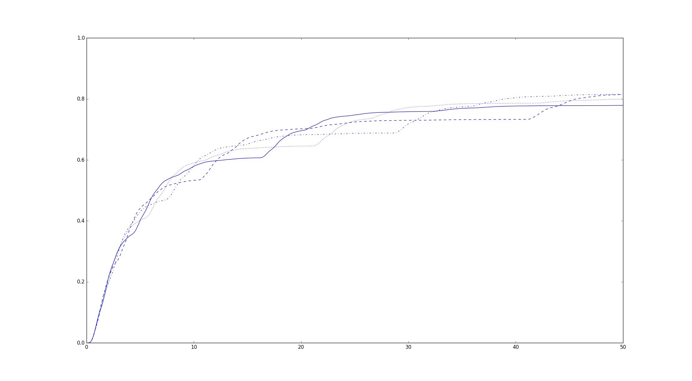
Figure 1: The $G_{\lambda}$ functions in the St. Petersburg case $\alpha=0.5$.

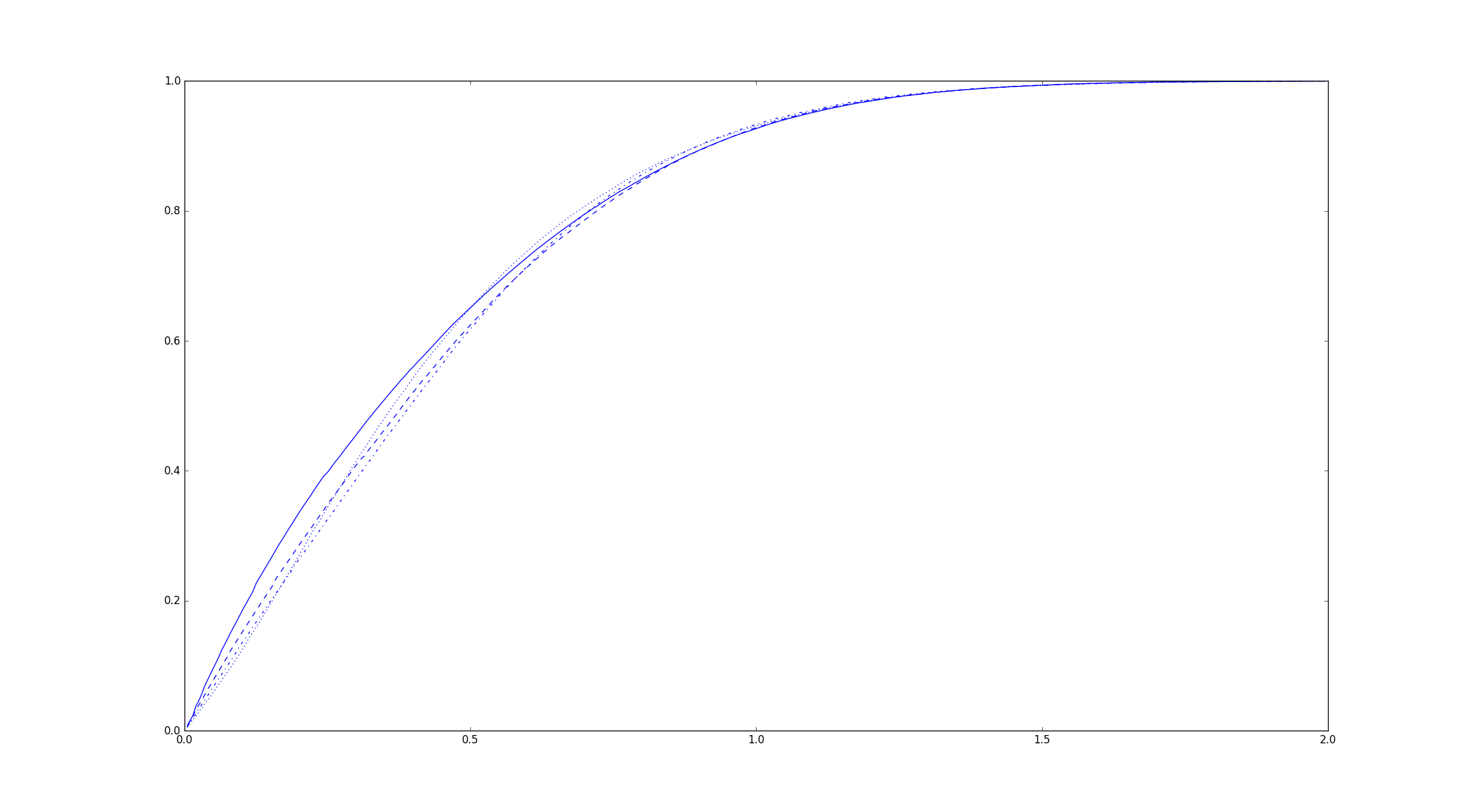
Figure 2: The $H_{\lambda}$ functions in the St. Petersburg case $\alpha=0.5$.

5 On the renewal measure

The aim of this section is to provide asymptotics for the renewal measure of the return times when the underlying distribution belongs to the domain of geometric partial attraction of a semistable law. We extend the result for positive operators in the spirit of Melbourne and Terhesiu [29], which is a crucial step in Section 7 to obtain limit theorems for a dynamical system, which is not isomorphic to a Markov renewal chain.

5.1 Scalar case

First, we need several definitions and results about regularly log-periodic functions; see [23]. Introduce the set of logarithmically periodic functions with period $r>1$

$$\begin{split}\mathcal{P}_{r}=\Big{\{}p:(0,\infty)\to(0,\infty):&\,\inf_{x\in[1,r]}p(x)>0,\ p\text{ is bounded, right-continuous, }\\ &\text{ and }p(xr)=p(x),\ \forall x>0\Big{\}}.\end{split}$$

Since we need monotonicity, for $r>1$ we further introduce the sets of functions

$$\begin{split}&\mathcal{P}_{r,\rho}=\Big{\{}p:(0,\infty)\to(0,\infty)\,:\,p\in\mathcal{P}_{r},\text{ and }x^{\rho}p(x)\text{ is nondecreasing}\Big{\}},\ \rho\geq 0,\\ &\mathcal{P}_{r,\rho}=\Big{\{}p:(0,\infty)\to(0,\infty)\,:\,p\in\mathcal{P}_{r},\text{ and }x^{\rho}p(x)\text{ is nonincreasing}\Big{\}},\ \rho<0.\end{split}$$ (5.1)

We also need results on the Laplace–Stieltjes transform of regularly log-periodic functions. Therefore, for $r>1$, $\rho\geq 0$, put

$$\begin{split}\mathcal{Q}_{r,\rho}=\Big{\{}q:&(0,\infty)\to(0,\infty)\,:\,q\in\mathcal{P}_{r},\text{ and }s^{-\rho}q(s)\text{ is completely monotone}\Big{\}}.\end{split}$$

Define the operator $\mathrm{A}_{\rho}:\mathcal{P}_{r,\rho}\to\mathcal{Q}_{r,\rho}$, $\rho>0$, as

$$\mathrm{A}_{\rho}p(s)=s^{\rho}\int_{0}^{\infty}e^{-sx}\mathrm{d}(p(x)x^{\rho}).$$ (5.2)

In Lemma 1 in [23] it is shown that $\mathrm{A}_{\rho}$ is one-to-one.

Let $\mathcal{P}_{r,\rho}^{1}$ denote the set of differentiable functions in $\mathcal{P}_{r,\rho}$. For $r>1$ and $\rho>0$ introduce the operator $\mathrm{B}_{r,\rho}=\mathrm{B}_{\rho}:\mathcal{P}_{r}\to\mathcal{P}_{r,\rho}^{1}$

$$\mathrm{B}_{\rho}p(x)=x^{-\rho}\int_{0}^{x}y^{\rho-1}p(y)\mathrm{d}y.$$ (5.3)

Then $\mathrm{B}_{\rho}$ is one-to-one with inverse

$${\mathrm{B}}_{\rho}^{-1}q(x)=x^{1-\rho}\frac{\mathrm{d}}{\mathrm{d}x}[x^{\rho}q(x)],\quad q\in\mathcal{P}_{r,\rho}^{1}.$$

In this section we assume that the subsequence $k_{n}$ in (2.1) is $k_{n}=\lfloor c^{n}\rfloor$ and (2.6) holds with $\ell\equiv 1$. The latter is equivalent to $\ell_{1}\sim 1$ by (2.5). It is easy to see that in this case $\delta(x)$ can indeed be replaced by $x$ in (2.6). Therefore

$$\overline{F}(x)=x^{-\alpha}\left(M(x)+h(x)\right),\quad k_{n}=\lfloor c^{n}\rfloor,$$ (5.4)

where $M(xc^{1/\alpha})=M(x)$ for all $x>0$, i.e. $M\in\mathcal{P}_{c^{1/\alpha}}$, and $\lim_{n\to\infty}h(xc^{n/\alpha})=0$ for all $x\in C_{M}$, with $C_{M}$ being the continuity points of $M$.

The renewal function corresponding to $F$ is defined as

$$U(x)=\sum_{n=0}^{\infty}F^{*n}(x),$$

where $F^{*n}$ stands for the $n$th convolution power.

Proposition 5.1

Assume (5.4). Then

$$\lim_{n\to\infty}\frac{U(c^{n/\alpha}z)}{c^{n}z^{\alpha}}=p(z),\quad z\in C_{p},$$ (5.5)

with $p=\mathrm{A}^{-1}_{\alpha}({1}/{\mathrm{A}_{1-\alpha}\mathrm{B}_{1-\alpha}M})$.

If $p$ is continuous, then (5.5) implies

$$U(x)\sim x^{\alpha}p(x)\quad\text{as }x\to\infty.$$

Proof.

From (5.4)

$$\lim_{n\to\infty}{c^{n}z^{\alpha}}\overline{F}(c^{n/\alpha}z)=M(z),\quad z\in C_{M}.$$

Corollary 1 in [23] implies that

$$1-\widehat{F}(s)=\int_{0}^{\infty}(1-e^{-sy})\mathrm{d}F(y)\sim s^{\alpha}q_{0}(s),$$ (5.6)

where $q_{0}=\mathrm{A}_{1-\alpha}\mathrm{B}_{1-\alpha}M$.

Thus, using (5.6) for the Laplace transform of $U$ we obtain as $s\downarrow 0$

$$\begin{split}\widehat{U}(s)&=\int_{0}^{\infty}e^{-sy}\mathrm{d}U(y)=\sum_{n=0}^{\infty}\left(\widehat{F}(s)\right)^{n}\\ &=\frac{1}{1-\widehat{F}(s)}\sim\frac{1}{s^{\alpha}q_{0}(s)}.\end{split}$$

By Theorem 1 in [23] the latter is equivalent to (5.5) with $\mathrm{A}_{\alpha}p=1/q_{0}$, and the statement follows. ∎

5.2 Operator case

We recall that in the set-up of Subsections 1.2 and 1.3, we have $u_{n}=L^{n}1_{Y}$, a.e. on $Y$, where $L$ is the transfer operator associated with $(X,\mathcal{B}_{X},T,\mu)$. We assume that (5.4) holds for the distribution function of $\tau$, which by Proposition 5.1, implies (5.5). As a consequence,

$$\lim_{n\to\infty}\frac{\sum_{j=0}^{[c^{n/\alpha}z]}u_{j}}{c^{n}z^{\alpha}}=\lim_{n\to\infty}\frac{\sum_{j=0}^{[c^{n/\alpha}z]}L^{n}1_{Y}}{c^{n}z^{\alpha}}=p(z),\quad z\in C_{p}.$$ (5.7)

In what follows we are interested in a more general form of (5.7) that applies to dynamical system that do not come equipped with an iid sequence $\{\tau\circ T_{Y}^{n}\}_{n\geq 1}$ and for which (1.5) does not hold. We consider such dynamical systems in Section 7, where we justify that Theorem 5.2 below (a generalisation of (5.7)) applies to them.

Before stating the result of this section, we recall the following notation: we write $T(x)\sim c(x)P$ for bounded operators $T(x),P$ acting on some Banach space ${\mathcal{B}}$ with norm $\|\,\|$ if $\|T(x)-c(x)P\|=o(c(x))$.

Theorem 5.2

Set $\hat{T}(e^{-s})=\sum_{n=0}^{\infty}T_{n}e^{-sn}$, $s>0$, where $T_{n}$ are uniformly bounded positive operators on some Banach space ${\mathcal{B}}$ with norm $\|\,\|$. Let $P:{\mathcal{B}}\to{\mathcal{B}}$ be a bounded linear operator. Assume that

$$\hat{T}(e^{-s})\sim\frac{1}{s^{\alpha}\ell(1/s)q_{0}(s)}P\text{ as }s\to 0,$$ (5.8)

for some slowly varying function $\ell$, $\alpha\in(0,1)$, and $q_{0}\in\mathcal{Q}_{c^{1/\alpha},\alpha}$. Let $p=\mathrm{A}_{\alpha}^{-1}(1/q_{0})$. Then for all $z\in C_{p}$, as $n\to\infty$,

$$\sum_{j=0}^{\lfloor c^{n/\alpha}z\rfloor}T_{j}\sim\frac{c^{n}z^{\alpha}}{\ell(c^{n/\alpha}z)}\,p(z)\,P.$$

Proof.

Given assumption (5.8), we proceed as in the proofs of [30, Proposition 3.3 and Lemma 3.5], which adapt the proof of Karamata’s theorem via ‘approximation by polynomials’ (see, for instance, Korevaar [25, Section 1.11]) to the case of positive operators.

Step 1 Given a polynomial $Q(x)=\sum_{k=1}^{m}b_{k}x^{k}$, we argue that

$$\sum_{j=0}^{\infty}T_{j}Q(e^{-sj})\sim\frac{1}{s^{\alpha}\ell(1/s)}\int_{0}^{\infty}Q(e^{-x})\,\mathrm{d}(p(x/s)x^{\alpha})P.$$ (5.9)

Note that

$$\hat{T}(e^{-s})\sim\frac{1}{s^{\alpha}\ell(1/s)q_{0}(s)}P=\frac{1}{s^{\alpha}\ell(1/s)}\mathrm{A}_{\alpha}p(s)P=\frac{1}{\ell(1/s)}\int_{0}^{\infty}e^{-sx}\,\mathrm{d}(p(x)x^{\alpha})P$$

and that $\sum_{j=0}^{\infty}T_{j}Q(e^{-sj})=\sum_{k=1}^{m}b_{k}\sum_{j=0}^{\infty}T_{j}e^{-sjk}=\sum_{k=1}^{m}b_{k}\hat{T}(e^{-sk})$. Now, for $k\in{\mathbb{N}}$,

$$\hat{T}(e^{-sk})\sim\frac{1}{\ell(1/s)}\int_{0}^{\infty}e^{-skx}\,\mathrm{d}(p(x)x^{\alpha})P=\frac{1}{s^{\alpha}\ell(1/s)}\int_{0}^{\infty}e^{-kx}\,\mathrm{d}(p(x/s)x^{\alpha})P.$$

Hence, (5.9) follows from the previous displayed equation after multiplication with $b_{k}$ and summation over $k$.

Step 2 Let $g=1_{[e^{-1},1]}$. Let $\varepsilon>0$ be arbitrary and let $z$ be a continuity point of $p$. Therefore we can choose a $\delta>0$ such that

$$p((1+\delta)z)(1+\delta)^{\alpha}-p((1-\delta)z-)(1-\delta)^{\alpha}<\frac{\varepsilon}{2}.$$ (5.10)

By Lemma 8.1 in Appendix 8.3, for these $\varepsilon$ and $\delta$ we can choose a polynomial $Q$ such that $Q\geq g$ on $[0,1]$ and for any measure $\mu$ on $(0,\infty)$ such that $\int_{0}^{\infty}e^{-x}\mu(\mathrm{d}x)<\infty$,

$$\int_{0}^{\infty}\left[Q(e^{-x})-g(e^{-x})\right]\mu(\mathrm{d}x)\leq\varepsilon\int_{0}^{\infty}e^{-x}\mu(\mathrm{d}x)+\mu((1-\delta,1+\delta)).$$ (5.11)

Using that $Q\geq g$ and (5.9), we obtain

$$\sum_{j=0}^{\lfloor c^{n/\alpha}z\rfloor}T_{j} =\sum_{j=0}^{\infty}T_{j}g\Big{(}e^{-\frac{j}{\lfloor c^{n/\alpha}z\rfloor}}\Big{)}$$

$$\leq\sum_{j=0}^{\infty}T_{j}Q\Big{(}e^{-\frac{j}{\lfloor c^{n/\alpha}z\rfloor}}\Big{)}$$

$$\sim\frac{c^{n}z^{\alpha}}{\ell(c^{n/\alpha}z)}\int_{0}^{\infty}Q(e^{-x})\mathrm{d}(p(x\lfloor c^{n/\alpha}z\rfloor)x^{\alpha})\,P.$$

We apply (5.11) for the measure $\mu_{n}(\mathrm{d}x)=\mathrm{d}(p(x\lfloor c^{n/\alpha}z\rfloor)x^{\alpha})$. Since $p$ is bounded

$$\sup_{n\geq 1}\int_{0}^{\infty}e^{-x}\mathrm{d}(p(x\lfloor c^{n/\alpha}z\rfloor)x^{\alpha})=:K<\infty.$$ (5.12)

Using the monotonicity of $p(x)x^{\alpha}$, the logarithmic periodicity of $p$, and (5.10)

$$\begin{split}\mu_{n}((1-\delta,1+\delta))&\leq p((1+\delta)\lfloor c^{n/\alpha}z\rfloor)(1+\delta)^{\alpha}-p((1-\delta)\lfloor c^{n/\alpha}z\rfloor)(1-\delta)^{\alpha}\\ &=(\lfloor c^{n/\alpha}z\rfloor)^{-\alpha}\Big{[}p((1+\delta)\lfloor c^{n/\alpha}z\rfloor)((1+\delta)\lfloor c^{n/\alpha}z\rfloor)^{\alpha}\\ &\qquad-p((1-\delta)\lfloor c^{n/\alpha}z\rfloor)((1-\delta)\lfloor c^{n/\alpha}z\rfloor)^{\alpha}\Big{]}\\ &\leq(\lfloor c^{n/\alpha}z\rfloor)^{-\alpha}\Big{[}p((1+\delta)c^{n/\alpha}z)((1+\delta)c^{n/\alpha}z)^{\alpha}\\ &\qquad-p((1-\delta)(c^{n/\alpha}z-1))((1-\delta)(c^{n/\alpha}z-1))^{\alpha}\Big{]}\\ &\rightarrow p((1+\delta)z)(1+\delta)^{\alpha}-p((1-\delta)z-)(1-\delta)^{\alpha}<\frac{\varepsilon}{2}.\end{split}$$

Thus for $n$ large enough

$$\mu_{n}((1-\delta,1+\delta))<\varepsilon.$$ (5.13)

Thus, using (5.11), (5.12), (5.13), and that $z$ is a continuity point of $p$, for $n$ large enough

$$\begin{split}\int_{0}^{\infty}Q(e^{-x})\mathrm{d}(p(x\lfloor c^{n/\alpha}z\rfloor)x^{\alpha})&\leq\int_{0}^{\infty}g(e^{-x})\mathrm{d}(p(x\lfloor c^{n/\alpha}z\rfloor)x^{\alpha})+\varepsilon(K+1)\\ &\leq p(z)+\varepsilon(K+2).\end{split}$$

Reverse inequality can be shown similarly. Thus the conclusion follows since $\varepsilon>0$ is arbitrary. ∎

6 Examples of null recurrent renewal shifts satisfying tail condition (2.6)

In this section we construct three dynamical systems that can be modelled by null recurrent renewal shifts (as described in Section 1) that satisfy tail condition (2.6). As such, we justify that Theorem 3.1 (describing the distributional behaviour of $S_{n_{r}}$) and Proposition 5.1 (and thus (5.7), describing the limit behaviour of the average transfer operator $\sum_{j=0}^{[c^{n/\alpha}z]}L^{j}1_{Y}$) apply to these examples. We recall that dynamical systems that can be modelled by null recurrent renewal shifts have the property that the sequence $\{\tau\circ T_{Y}^{n}\}_{n\geq 1}$ is iid.

The first two examples in Subsections 6.1 and 6.2 can be regarded as perturbations of the intermittent map with linear branches preserving an infinite measure, known as Wang map (Gaspard and Wang [16]); an exact form of a (unperturbed) Wang type map $T_{0}:[0,1]\to[0,1]$ in terms of the parameter $\alpha>0$ is given by (6.3) with $\varepsilon=0$. We recall that $T_{0}$ is a linear version of the smooth intermittent map studied by Pomeau and Manneville [31] with $T_{0}^{\prime}(x)>1$ for all $x\in(0,1]$ and $T_{0}^{\prime}(0)=1$ (so, it is expanding everywhere, but at the so-called indifferent fixed point $0$). When $\alpha<1$, the map $T_{0}$ preserves an infinite measure, equivalently it is a null recurrent renewal chain, where the first return $\tau$ to $Y=[1/2,1]$ satisfies strict regular variation: $m(\tau>n)=\frac{1}{2}n^{-\alpha}$ for the normalised Lebesgue measure $m$ on $Y=[\frac{1}{2},1]$. We recall that this strict regular variation implies that $T_{0}$ satisfies a Darling–Kac law and that $n^{-\alpha}\sum_{j=0}^{n}L^{j}1_{Y}\to C$, a.e. on $Y$, as $n\to\infty$, for some $C>0$ (depending only on the parameters of $T_{0}$).

As clarified in subsections 6.1 and 6.2 a slight perturbation of $T_{0}$ gives rise to different tails $m(\tau>n)$, which are no longer regularly varying. Instead, we show that $m(\tau>n)$ satisfies tail condition (2.6) with a continuous and a noncontinuous, respectively, logarithmic periodic function $M$ (identifying the involved sequence $k_{n}$). Moreover, while the map in subsection 6.1 is differentiable at $0$ from the right (so, $0$ is an indifferent fixed point), the map in subsection 6.2 is not differentiable at $0$; for this second example we justify that we can still speak of ‘the derivative at $0$ along subsequences’ being equal to $1$ (see equation (6.2) and text before it).

In subsection 6.3, we introduce a family of maps $T_{\lambda}$ (as in (6.7)) generated out of the sequence of Fibonacci numbers, somewhat similar to, but simpler in structure than, the maps studied by Bruin and Todd in [7, 8]. In short, the maps $T_{\lambda}$ are Kakutani towers over linear maps (as in (6.6)) generated out of the Fibonacci sequence. As such, they are isomorphic to renewal shifts and equation (6.8) says that they are null recurrent renewal shifts. As shown in Proposition 6.1, the maps $T_{\lambda}$ satisfy tail condition (2.6), identifying the involved sequence $k_{n}$. This justifies that Theorem 3.1 applies to $T_{\lambda}$. Moreover, the form of the sequence $k_{n}$ in Proposition 6.1 allows for an immediate application of Proposition 5.1 and thus (5.7) (see text after the proof of Proposition 6.1).

We believe that Proposition 6.1 together with Theorem 8.14 by Bruin et al. [6] can be used to show that Theorem 3.1 applies to the family of countably piecewise linear (unimodal) maps with Fibonacci combinatorics studied in [7, 8]. For simplicity of the exposition, in this work we restrict to the self-contained model introduced in subsection 6.3.

6.1 First perturbation of the Wang map: continuous case

Fix $\alpha\in(0,1)$, $c>1$, $\varepsilon>0$ and for $n\geq 1$, define

$$\xi_{n}=\frac{1}{2}n^{-\alpha}\left(1+2\varepsilon\sin\left(\frac{2\pi\alpha\log n}{\log c}\right)\right).$$ (6.1)

Note that $\xi_{1}=\frac{1}{2}$. First we show that $\xi_{n}$ is strictly decreasing. Let

$$M(x)=\frac{1}{2}\left(1+2\varepsilon\sin\left(\frac{2\pi\alpha\log x}{\log c}\right)\right).$$ (6.2)

Then $M$ is bounded and bounded away from zero for $\varepsilon<\frac{1}{2}$, and $M(c^{1/\alpha}x)=M(x)$ for all $x\in(0,\infty)$. Furthermore $R(x):=-M(x)x^{-\alpha}$ is continuous and nondecreasing for small $\varepsilon$. Indeed, short calculation shows that $R^{\prime}(x)=2^{-1}x^{-(1+\alpha)}(\alpha+O(\varepsilon))$, where $|O(\varepsilon)|\leq 2\alpha\varepsilon(1+2\pi/\log c)$. This implies that $\xi_{n}=-R(n)$ in (6.1) is decreasing, whenever $\varepsilon>0$ is small enough, which we assume in the following.

Set $\xi_{0}=1$, and define a countably piecewise linear map

$$T_{\varepsilon}(x)=\begin{cases}\frac{\xi_{n}-x}{\xi_{n}-\xi_{n+1}}\xi_{n}+\frac{x-\xi_{n+1}}{\xi_{n}-\xi_{n+1}}\xi_{n-1},&\text{ for }x\in[\xi_{n+1},\xi_{n}],n\geq 1,\\ 2x-1,&\text{ for }x\in(\frac{1}{2},1].\end{cases}$$ (6.3)

Then $T_{\varepsilon}(\xi_{n})=\xi_{n-1}$ for $n\geq 1$, and the graph of $T_{\varepsilon}$ consists of line segments connecting the points $(\xi_{n},\xi_{n-1})\in[0,1]$ for $n\geq 1$, as well as $(\frac{1}{2},0)$ to $(1,1)$. For $\varepsilon=0$ we have exactly the Wang map $T_{0}$. The graph of $T_{\varepsilon}$ for $\varepsilon>0$ has Hausdorff distance $\leq\varepsilon$ to the graph of $T_{0}$ and thus, $\|T_{\varepsilon}-T_{0}\|_{\infty}\leq\varepsilon$.

Straightforward calculation shows that

$$\begin{split}\Delta\xi_{n}&:=\xi_{n}-\xi_{n+1}\\ &=\frac{\alpha n^{-\alpha-1}}{2}\left[1+2\varepsilon\sin\left(\frac{2\pi\alpha}{\log c}\log n\right)-\frac{4\pi\varepsilon}{\log c}\cos\left(\frac{2\pi\alpha}{\log c}\log n\right)\right]+O(n^{-2-\alpha}),\end{split}$$ (6.4)

from which we see that $T_{\varepsilon}$ is differentiable at 0 from the right, and

$$T_{\varepsilon}^{\prime}(0)=1,$$

so 0 is an indifferent fixed point.

Let $\tau$ be the first return time to $[1/2,1]$. We see that for $n\geq 1$, $\{\tau=n+1\}=((1+\xi_{n+1})/2,(1+\xi_{n})/2]$, thus

$$m(\tau>n)=\sum_{j\geq n}\Delta\xi_{n}=\xi_{n}=\frac{1}{2}n^{-\alpha}\left(1+2\varepsilon\sin\left(\frac{2\pi\alpha\log n}{\log c}\right)\right),$$

where $m$ is the normalised Lebesgue measure on $Y=[\frac{1}{2},1]$.

Define $k_{n}=\lfloor c^{n}\rfloor$, $\ell\equiv 1$ and $A_{k}=k^{1/\alpha}$, so $A_{k_{n}}=\lfloor c^{n}\rfloor^{1/\alpha}$. In this case $\delta(x)$ can be simply changed to $x$ in (2.6). Thus $\tau$ satisfies (2.6) with $M$ in (6.2).

Figures 3 and 4 show the limiting $G_{\lambda}$ and $H_{\lambda}$ functions for the parameter values $\alpha=0.5$, $\varepsilon=0.04$, and $c=2$. The distribution function is calculated numerically from the characteristic function using the Gil-Pelaez–Rosén inversion formula [17, 32].

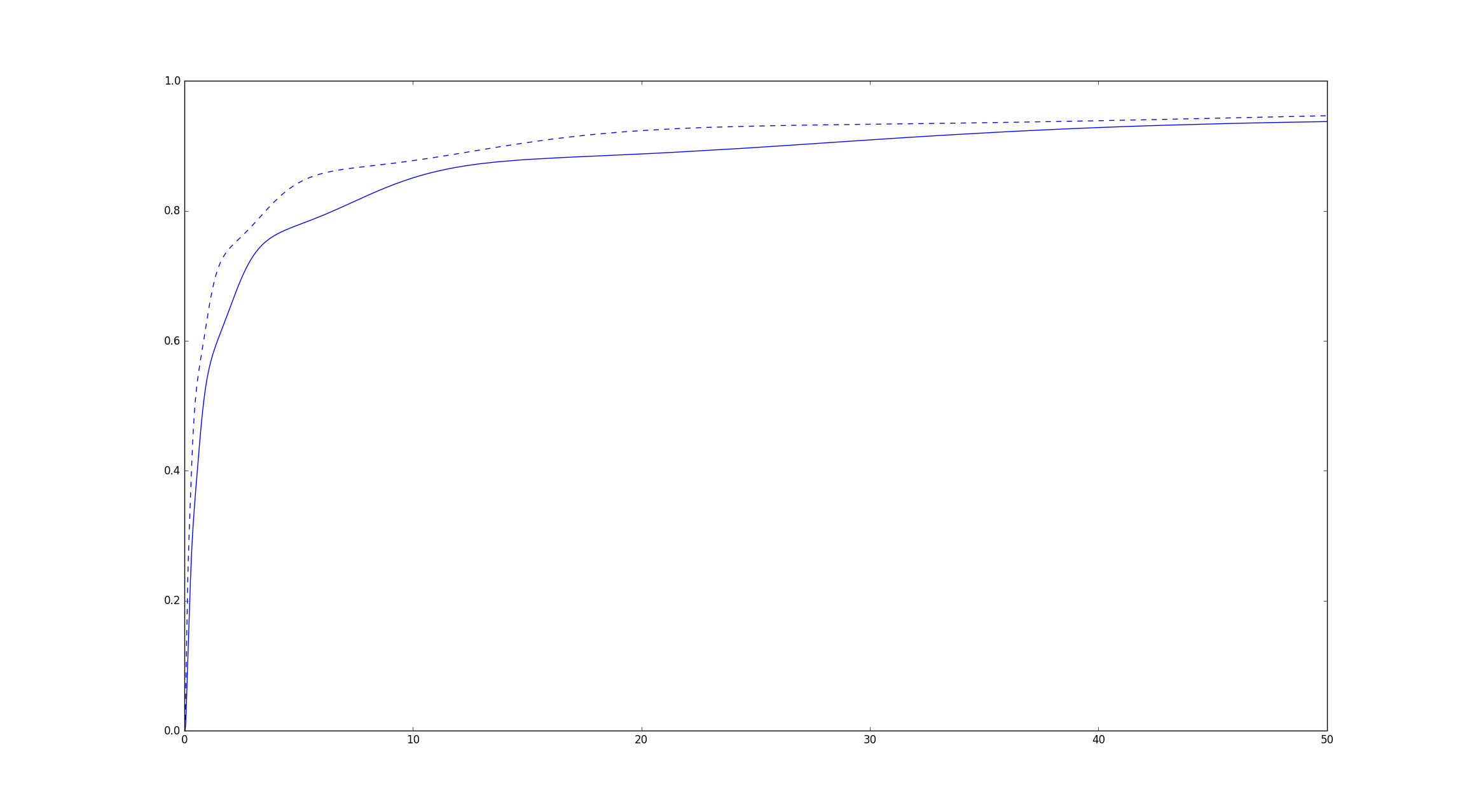
Figure 3: The distribution functions $G_{0.5}$ (solid) and $G_{0.75}$ (dashed).

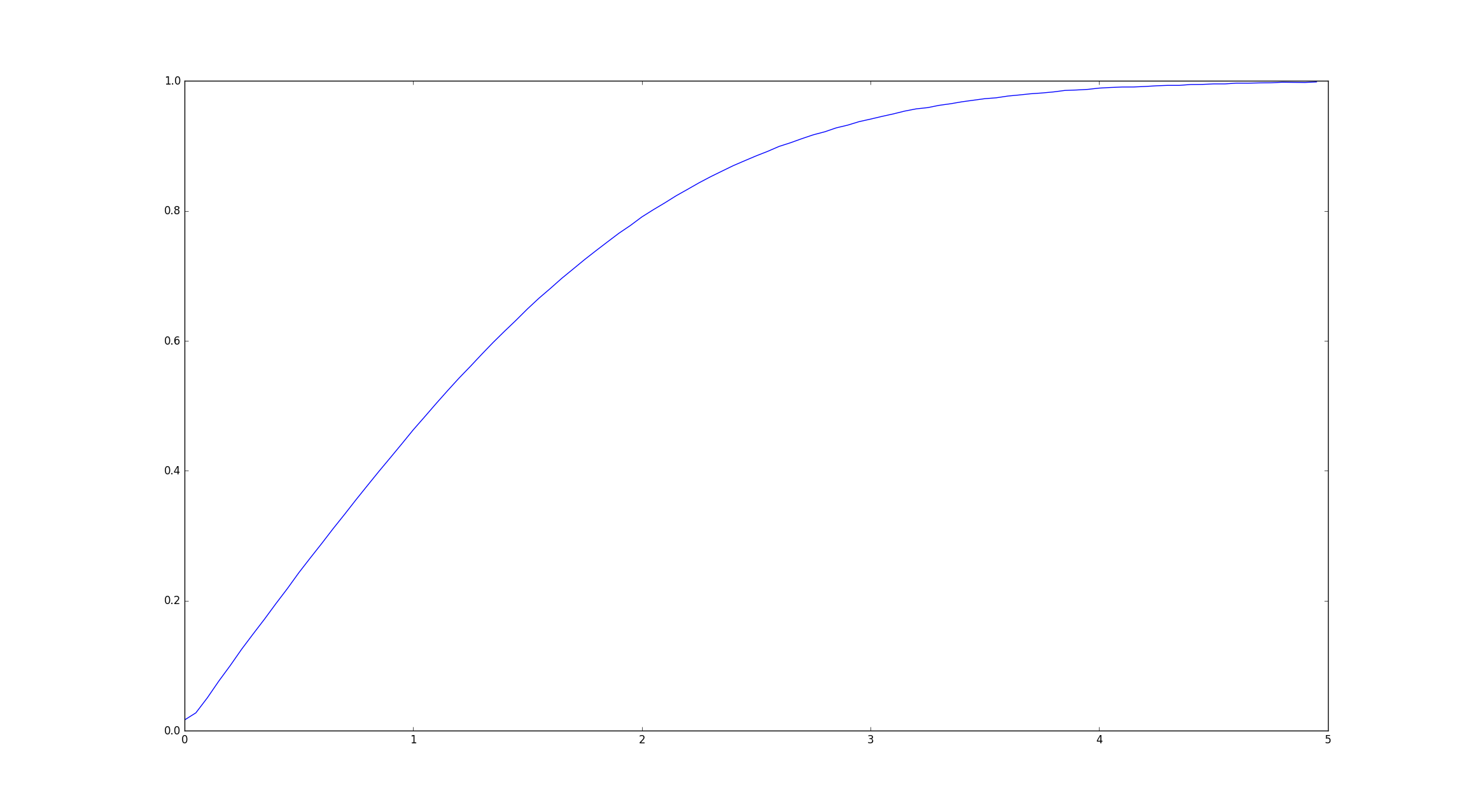
Figure 4: The $H_{1}$ function.

6.2 Second perturbation of the Wang map: noncontinuous case

The resulting distribution for the example in this section is not exactly the generalised St. Petersburg distribution, but it is similar to it. We proceed as in the previous section, but this time suppose that

$$\xi_{n}=\frac{1}{2}n^{-\alpha}(1+2^{\{\alpha\log_{2}n\}}),\ n\geq 1,$$

and set $\xi_{0}=1$. As before, $\{\cdot\}$ stands for the fractional part. It is easy to see that $\xi_{n}$ is strictly decreasing. Define

$$T(x)=\begin{cases}\frac{\xi_{n}-x}{\xi_{n}-\xi_{n+1}}\xi_{n}+\frac{x-\xi_{n+1}}{\xi_{n}-\xi_{n+1}}\xi_{n-1},&\text{for }x\in[\xi_{n+1},\xi_{n}],\ n\geq 1,\\ 2x-1,&\text{ for }x\in(\frac{1}{2},1].\end{cases}$$

and note that $T(\xi_{n+1})=\xi_{n}$ for all $n$. It turns out that the derivative at $0$ does not exist. Indeed,

$$\frac{T(\xi_{n+1})}{\xi_{n+1}}=\frac{\xi_{n}}{\xi_{n+1}}=\frac{(n+1)^{\alpha}}{n^{\alpha}}\frac{1+2^{\{\alpha\log_{2}n\}}}{1+2^{\{\alpha\log_{2}(n+1)\}}}.$$

Clearly $\frac{(n+1)^{\alpha}}{n^{\alpha}}\to 1$, but $\frac{1+2^{\{\alpha\log_{2}n\}}}{1+2^{\{\alpha\log_{2}(n+1)\}}}$ is only close to $1$ if there is no integer between $\alpha\log_{2}n$ and $\alpha\log_{2}(n+1)$. Equivalently $n\neq\lfloor 2^{k/\alpha}\rfloor$ for any integer $k$. Thus, the sequence $(T(\xi_{n})/\xi_{n})$ has two limit points, 1 and $3/2$:

$$1=\liminf_{x\downarrow 0}\frac{T(x)}{x}<\limsup_{x\downarrow 0}\frac{T(x)}{x}=\frac{3}{2}.$$

Although the derivative at $0$ does not exist, we can still speak of the ‘derivative at $0$ along subsequences’. Indeed, if $(n_{j})$ is any increasing sequence taking values in ${\mathbb{N}}\setminus\{\lfloor 2^{k/\alpha}\rfloor:k\in{\mathbb{N}}\}$, then $\lfloor\alpha\log_{2}n_{j}\rfloor=\lfloor\alpha\log_{2}(n_{j}+1)\rfloor$. Therefore, $\{\alpha\log_{2}n_{j}\}-\{\alpha\log_{2}(n_{j}+1)\}\to 0$, and

$$\lim_{j\to\infty}\frac{1+2^{\{\alpha\log_{2}n_{j}\}}}{1+2^{\{\alpha\log_{2}(n_{j}+1)\}}}=1.$$

Again, let $\tau$ be the first return time to $[1/2,1]$, and $m$ the normalised Lebesgue measure on $[1/2,1]$. For $n\geq 1$, $m(\tau=n+1)=\Delta\xi_{n}=\xi_{n}-\xi_{n-1}$, thus

$$m(\tau>n)=\sum_{j\geq n}\Delta\xi_{n}=\xi_{n}=\frac{1}{2}n^{-\alpha}\left(1+2^{\{\alpha\log_{2}n\}}\right).$$

Thus $\tau$ satisfies (2.6) with $\ell^{*}\equiv 1$, $M(x)=(1+2^{\{\alpha\log_{2}x\}})/2$, $k_{n}=2^{n}$, and $c=2$. Again $\delta(x)$ is changed to $x$. We have $M(2^{1/\alpha}x)=M(x)$ for all $x\in(0,\infty)$, as required.

6.3 Piecewise linear maps generated out of the Fibonacci sequence

Denote the sequence of Fibonacci numbers by $\{S_{0},S_{1},S_{2},S_{3},\dots\}=\{1,2,3,5,\dots\}$. From Binet’s formula, we get

$$S_{n}=\frac{1}{\sqrt{5}}(G^{n+2}-(-G)^{-n-2})=q_{0}(1-(-1)^{n}G^{-2(n+2)})\,G^{n},$$ (6.5)

where $G=\frac{1+\sqrt{5}}{2}$ is the golden mean and $q_{0}=\frac{3+\sqrt{5}}{2\sqrt{5}}$.

Fix $\lambda\in(1/G,1)$, let $Y=[0,1]$ and define $T_{Y,\lambda}:Y\to Y$ by $T_{Y,\lambda}(0)=0$ and

$$T_{Y,\lambda}(y)=\frac{\lambda^{n}-y}{\lambda^{n}-\lambda^{n+1}}\qquad y\in(\lambda^{n+1},\lambda^{n}].$$ (6.6)

The map $T_{Y,\lambda}$ preserves the Lebesgue measure $m$. Given the probability preserving transformation $(Y,{\mathcal{B}}(Y),m,T_{Y,\lambda})$ and a measurable function $\tau:Y\to{\mathbb{N}}$ we construct the Kakutani tower/map $(X,{\mathcal{B}}(X),\mu,T_{\lambda})$ (see, for instance, [1, Chapter 5] and references therein) as follows.

Let

• $X:=\cup_{n\geq 1}\left(\{\tau\geq n\}\times\{n\}\right)$;

• $\mathcal{B}(X):=\sigma\left(C_{n}\times\{n\}:\,C_{n}\in{\mathcal{B}}(Y)\cap\{\tau\geq n\}\ \text{for all }n\geq 1\right)$;

• for all $A\in({\mathcal{B}}(Y)\cap\{\tau\geq n\})$, set $\mu(A\times\{n\})=m(A)$.

Given $T_{Y,\lambda}$ introduced in (6.6), define the tower map $T_{\lambda}:X\to X$ by

$$T_{\lambda}(x,n)=\begin{cases}(y,n+1),&\tau(y)>n,\\ (T_{Y,\lambda}(y),1),&\tau(y)=n.\end{cases}$$ (6.7)

By construction, $T_{\lambda}$ preserves $\mu$. Moreover, $\tau$ is the first return time of $T_{\lambda}$ to the base $Y\times\{1\}$ and $T_{\lambda}^{\tau(y)}(y,1)=(T_{Y,\lambda}(y),1)$. In what follows, we set $\tau(y)=S_{n}$ for $y\in(\lambda^{n+1},\lambda^{n}]$, so

$$m(\tau=S_{n})=(1-\lambda)\lambda^{n}.$$ (6.8)

We shall show that $m(\tau>x)$ satisfies (2.6).

By (6.8), for $S_{n}\leq x<S_{n+1}$, we have

$$m(\tau>x)=m(\tau\geq S_{n+1})=\sum_{j\geq n+1}\mu(\tau=S_{j})=(1-\lambda)\sum_{j\geq n+1}\lambda^{j}=q_{n}S_{n}^{-\alpha},$$

where $\alpha=-\log_{G}\lambda$ and

$$q_{n}=\lambda\left(\frac{3+\sqrt{5}}{2\sqrt{5}}\right)^{\alpha}(1-(-1)^{n}G^{-2(n+2)})^{\alpha}.$$

We can easily see that

$$\lim_{n\to\infty}q_{n}=\lambda\left(\frac{3+\sqrt{5}}{2\sqrt{5}}\right)^{\alpha}=:q_{\infty}>0.$$

Moreover, since $\lambda\in(1/G,1)$, we have $\alpha\in(0,1)$. Since

$$S_{n}^{-\alpha}=x^{-\alpha}\left(\frac{x}{S_{n}}\right)^{\alpha}=x^{-\alpha}G^{\alpha\log_{G}\frac{x}{S_{n}}},$$

we have

$$m(\tau>x)=q_{n}x^{-\alpha}G^{\alpha\log_{G}\frac{x}{S_{n}}}\qquad\text{ for }S_{n}\leq x<S_{n+1}.$$ (6.9)

Equipped with the above, we state

Proposition 6.1

The tail of $\tau$ in (6.9) satisfies (2.6) with $c=G^{\alpha}$, $k_{n}=\lfloor G^{\alpha n}\rfloor$, $\ell(x)\equiv 1$, $A_{k}=k^{1/\alpha}$, and $M(x)=q_{\infty}G^{\alpha\{\log_{G}(x/q_{0})\}}$; i.e.

$$m(\tau>x)=x^{-\alpha}\left(M(x)+h(x)\right),$$

where $\lim_{n\to\infty}h(A_{k_{n}}x)=0$ whenever $x$ is continuity point of $M$.

Proof.

First recall again that if $\ell\equiv 1$ and $k_{n}=\lfloor c^{n}\rfloor$ then $\delta(x)$ in (2.6) can be replaced with $x$.

By (6.9) we may write

$$m(\tau>x)=x^{-\alpha}\left(q_{\infty}G^{\alpha\{\log_{G}\frac{x}{q_{0}}\}}+h(x)\right)$$

with

$$h(x)=q_{\infty}\left(G^{\alpha\log_{G}\frac{x}{S_{n}}}-G^{\alpha\{\log_{G}\frac{x}{q_{0}}\}}\right)+(q_{n}-q_{\infty})G^{\alpha\log_{G}\frac{x}{S_{n}}},\quad x\in[S_{n},S_{n+1}).$$ (6.10)

Therefore, we only have to prove that the error function $h$ satisfies the necessary properties in (2.6); i.e. $\lim_{n\to\infty}h(A_{k_{n}}x)=0$, whenever $x\in C_{M}$.

In (6.10) the second summand converges to 0 as $x\to\infty$. So we have to prove that for any $x\in C_{M}$

$$\lim_{n\to\infty}\log_{G}\frac{x\lfloor G^{\alpha n}\rfloor^{1/\alpha}}{S_{m}}=\left\{\log_{G}\frac{x}{q_{0}}\right\},$$

where $m=m_{n}$ is uniquely determined by $S_{m}\leq x\lfloor G^{\alpha n}\rfloor^{1/\alpha}<S_{m+1}$. This follows easily from (6.5) and that $x\in C_{M}$ if and only if $\{\log_{G}(x/q_{0})\}>0$. ∎

Proposition 6.1 shows that the return times corresponding to the map $T_{\lambda}$ satisfy tail condition (2.6). Hence, a semistable law for $(T_{Y,\lambda},\tau)$ holds along $k_{n}=\lfloor G^{\alpha n}\rfloor$. Thus, Theorem 3.1 applies to $T_{\lambda}$, giving the distributional behaviour of $S_{n_{r}}$, for suitable subsequences $n_{r}$. Moreover, since $k_{n}=\lfloor G^{\alpha n}\rfloor$, Proposition 5.1 (and thus (5.7)) holds.

7 A process, which is not isomorphic to a Markov renewal chain

In this section we show that (the conclusion of) Theorem 3.1 and Theorem 5.2 apply to infinite measure preserving systems that are not isomorphic to Markov renewal chains. To fix terminology, in Subsection 7.1 we provide a simple smooth version of the renewal shift (6.3) considered in Subsection 6.1; this is given by the family of smooth Markov maps $f_{\varepsilon}:[0,1]\to[0,1]$ (defined in (7.5)) with indifferent fixed point at $0$. In Subsection 7.2, we note that the first return time to a subset of $[0,1]$ satisfies the tail condition (2.6) and verify that the corresponding induced family of maps satisfy good distortion properties. The latter allows to conclude in Subsection 7.3 that the main functional analytical properties of the induced map hold and in Subsection 7.4 we justify that the conclusion of Theorem 3.1 holds for $f_{\varepsilon}$. Using the same functional analytic properties in Subsection 7.5 we show that Theorem 5.2 applies, obtaining the exact sequences and scaling for the convergence of the average transfer operator (7.11), uniformly on compacts of $(0,1]$. Finally, we mention that, although the results of this sections are in terms of a simple example, the same arguments apply to dynamical systems with infinite measure satisfying tail condition (2.6) along with properties (A1) and (A2) stated below. For a discussion of our results on infinite measure preserving systems we refer to Subsection 7.4.

7.1 A smooth version of the example in Subsection 6.1

For fixed $\alpha\in(0,1)$, $c>1$ and $\varepsilon$ small enough, we define $(\xi_{n})_{n\geq 0}$ as in Subsection 6.1, that is $\xi_{n}=\frac{1}{2}n^{-\alpha}\left(1+2\varepsilon\sin(\frac{2\pi\alpha\log n}{\log c})\right)$, $n\geq 2$ and $\xi_{0}=1$, $\xi_{1}=\frac{1}{2}$. We recall that, as clarified in Subsection 6.1, $\xi_{n}$ is decreasing. In what follows, out of $(\xi_{n})_{n\geq 0}$ we define a smooth map $f_{\varepsilon}:[0,1]\to[0,1]$ via the map $f_{\varepsilon,n}$ defined below.

A lengthy computation based on (6.4) (see Appendix 8.4 for details) shows that there exist $\alpha_{n}=(1+\alpha+O(n^{-1}))(1+O(\varepsilon))$ and $r_{n}=O(1)$ such that

$$\frac{\Delta\xi_{n-2}}{\Delta\xi_{n-1}}=\frac{\xi_{n-2}-\xi_{n-1}}{\xi_{n-1}-\xi_{n}}=1+\frac{\alpha_{n}}{n}+\frac{r_{n}}{n^{2}}+R_{n},$$ (7.1)

and $R_{n}=O(n^{-3})$. Let $f_{\varepsilon,n}:[\xi_{n},\xi_{n-1}]\to[\xi_{n-1},\xi_{n-2}]$, $n\geq 2$, be defined by

$$f_{\varepsilon,n}(x)=\frac{A_{n}}{2}\frac{(x-\xi_{n})^{2}}{\xi_{n-1}-\xi_{n}}+(1+\frac{\alpha_{n}}{n}+B_{n})(x-\xi_{n})+\xi_{n-1},$$

Here $A_{n}$ and $B_{n}$ will be chosen appropriately. We note that

$$f_{\varepsilon,n}(\xi_{n})=\xi_{n-1},\qquad f_{\varepsilon,n}(\xi_{n-1})=\xi_{n-2}.$$

The first is automatic, and the second follows provided

$$\frac{r_{n}}{n^{2}}+R_{n}=B_{n}+\frac{A_{n}}{2}.$$ (7.2)

The derivative is

$$f^{\prime}_{\varepsilon,n}(x)=\frac{x-\xi_{n}}{\xi_{n-1}-\xi_{n}}A_{n}+1+\frac{\alpha_{n}}{n}+B_{n}.$$

We note that

$$f^{\prime}_{\varepsilon,n}(\xi_{n})=1+\frac{\alpha_{n}}{n}+B_{n},\qquad f^{\prime}_{\varepsilon,n}(\xi_{n-1})=1+\frac{\alpha_{n-1}}{n-1}+B_{n-1}.$$

provided that (the first equation above is automatic)

$$A_{n}=\frac{\alpha_{n-1}}{n-1}-\frac{\alpha_{n}}{n}+B_{n-1}-B_{n},\quad n\geq 3.$$ (7.3)

Solving for $B_{n}$ from (7.2) and (7.3), we get the recursive formula

$$B_{n}=-B_{n-1}+\frac{2r_{n}}{n^{2}}+2R_{n}-\frac{\alpha_{n-1}}{n-1}+\frac{\alpha_{n}}{n}=:-B_{n-1}+q_{n},$$

for $q_{n}=\frac{2r_{n}}{n^{2}}+2R_{n}-\frac{\alpha_{n-1}}{n-1}+\frac{\alpha_{n}}{n}=O(n^{-2})$. Working out the recursion, we get

$$B_{n}=(-1)^{n}\left(B_{2}+\sum_{i=3}^{n}(-1)^{i}q_{i}\right),\quad i\geq 3,$$

for arbitrary $B_{2}\in{\mathbb{R}}$. Clearly, $(B_{n})_{n\geq 0}$ is bounded. Choose $B_{2}=-\sum_{i=3}^{\infty}(-1)^{i}q_{i}$. Then

$$B_{n}=(-1)^{n+1}\sum_{i=n+1}^{\infty}(-1)^{i}q_{i},\quad n\geq 3.$$ (7.4)

Note that

$$q_{n}-q_{n+1}=\left(\frac{2r_{n}}{n^{2}}-\frac{2r_{n+1}}{(n+1)^{2}}\right)+2(R_{n}-R_{n+1})-\left(\frac{\alpha_{n-1}}{n-1}-\frac{2\alpha_{n}}{n}-\frac{\alpha_{n+1}}{n+1}\right).$$

One can check that the $\alpha_{n}$’s and $r_{n}$’s change so slowly with $n$ that $q_{n}-q_{n+1}=O(n^{-3})$; see Appendix 8.4. Rewriting (7.4), we have

$$B_{n}=(-1)^{n+1}\sum_{k=1}^{\infty}\left[(-1)^{n+2k-1}q_{n+2k-1}+(-1)^{n+2k}q_{n+2k}\right]=\sum_{k=1}^{\infty}q_{n+2k-1}-q_{n+2k}=O(n^{-2}).$$

By (7.3), $A_{n}=O(n^{-2})$. Therefore $A_{n}$ and $B_{n}$ can be chosen appropriately.

Define the map $f_{\varepsilon}:[0,1]\to[0,1]$,

$$f_{\varepsilon}(x)=\begin{cases}f_{\varepsilon,n}(x),&x\in[\xi_{n},\xi_{n-1}],n\geq 2\\ 2x-1,&x>\frac{1}{2}.\end{cases}$$ (7.5)

By (6.4), we have that $f_{\varepsilon}$ is differentiable at $0$ (from the right) and $0$ is an indifferent fixed point.

7.2 Induced map, tail distribution, infinite invariant measure

Let $\tau$ be the first return time of $f_{\varepsilon}$ to $Y=[\frac{1}{2},1]$ and define the induced map $F_{\varepsilon}=f_{\varepsilon}^{\tau}$. Note that

$$F_{\varepsilon}:Y\to Y,\qquad F_{\varepsilon}(x)=\begin{cases}2x-1&\text{ if }x\in[\frac{3}{4},1],\\ f_{\varepsilon}^{n-1}(2x-1)&\text{ if }x\in[\frac{\xi_{n}+1}{2},\frac{\xi_{n-1}+1}{2}),n\geq 2,\\ \frac{1}{2}&\text{ if }x=\frac{1}{2},\end{cases}$$

has onto branches. In fact, as clarified below, the induced map $(Y,\mathcal{A}(Y),F_{\varepsilon},\gamma)$, where $\mathcal{A}(Y)$ the Borel sigma algebra on $Y$ and $\gamma=\{[\frac{\xi_{n}+1}{2},\frac{\xi_{n-1}+1}{2})\}_{n\geq 1}$, is Gibbs–Markov (for complete definitions see [2],  [1, Chapter 4]).

First, it follows from the above definition of $F_{\varepsilon}$ and $\gamma$ that each element of $\gamma$ is mapped bijectively onto a union of partition elements.

Next, differentiating $\Delta\xi_{n}$ in (6.4) w.r.t. $n$ gives that it is strictly decreasing in $n$, so $\Delta\xi_{n-2}/\Delta\xi_{n-1}>1$ and $f^{\prime}_{\varepsilon,n}(x)>1$ for all $x\in[\xi_{n},\xi_{n-1}]$. Moreover, $f^{\prime}_{\varepsilon}(x)=2$ on $(\frac{1}{2},1]$ by (7.5). By the chain rule we get $F^{\prime}(x)\geq 2$ as well for every $x\in(1/2,1]\setminus\{(\xi_{n}+1)/2\}_{n\geq 2}$. Thus, $F_{\varepsilon}$ is expanding on each element of its Markov partition $\gamma$. As a consequence, for every two points $x,y$ there exists $n\geq 0$ such that $F^{n}(x)$ and $F^{n}(y)$ lie in different elements of $\gamma$. Therefore, the atoms of the partition $\bigvee_{n=0}^{\infty}F^{-n}\gamma$ are points, which implies that $\gamma$ is a generating partition for $F_{\varepsilon}$ (that is, $\sigma(\{F_{\varepsilon}^{-n}\gamma:n\geq 0\})=\mathcal{A}(Y)$).

Also, by Lemma 8.2 in Appendix 8.4, $F_{\varepsilon}$ is piecewise $C^{2}$ and the distortion condition $\frac{|F_{\varepsilon}^{\prime\prime}|}{(F_{\varepsilon}^{\prime})^{2}}<\infty$ holds. The above verified properties, Markov generating partition, expansion and distortion conditions guarantees that $(Y,\mathcal{A}(Y),F_{\varepsilon},\gamma)$ is Gibbs–Markov. For the fact that the above distortion condition can be used as part of the definition of a Gibbs–Markov map, see [2, Example 2] and [1, Chapter 4].

Since $(Y,\mathcal{A}(Y),F_{\varepsilon},\gamma)$ is Gibbs–Markov, $F_{\varepsilon}$ preserves a measure $\mu_{Y}$ with density $h=\frac{\mathrm{d}\mu_{Y}}{\mathrm{d}m}$, with $m$ being the normalised Lebesgue measure on $Y$, bounded from above and below and $h\in C^{2}(Y)$ (see [2] and [1, Chapter 4]). Thus,

$$\mu_{Y}(\tau>n) =\int_{\frac{1}{2}}^{\frac{\xi_{n}+1}{2}}h(x)\,\mathrm{d}m(x)=h(1/2)\xi_{n}(1+o(1))$$

$$=\frac{1}{2}h(1/2)n^{-\alpha}\left(1+2\varepsilon\sin\left(\frac{2\pi\alpha\log n}{\log c}\right)\right)(1+o(1)).$$ (7.6)

An $f_{\varepsilon}$-invariant measure $\mu$ can be obtained by pulling back:

$$\mu(A)=\sum_{n\geq 0}\mu_{Y}(f^{-n}(A)\cap\{\tau>n\})$$

for every Borel measurable set $A$. Then $\mu([0,1])=\sum_{n\geq 0}\mu_{Y}(\{\tau>n\})=\infty$, so $\mu$ is infinite.

Similar to Subsection 6.1, we let $M(x)=\frac{1}{2}h(1/2)(1+2\varepsilon\sin(\frac{2\pi\alpha\log x}{\log c}))$, define $k_{n}=\lfloor c^{n}\rfloor$ and set $A_{k}=k^{1/\alpha}$, so $A_{k_{n}}=\lfloor c^{n}\rfloor^{1/\alpha}$. Thus, $\tau$ satisfies (2.6) with $\ell\equiv 1$.

7.3 Functional analytical properties of the induced map

Since it is not going to play a role, throughout the remaining of this section we suppress the dependency of the induced map on $\varepsilon$ and set $F:=F_{\varepsilon}$.

Let $R:L^{1}(\mu_{Y})\to L^{1}(\mu_{Y})$ be the transfer operator associated with $F:Y\to Y$ defined by $\int_{Y}R^{n}v\cdot w\,\mathrm{d}\mu_{Y}=\int_{Y}v\cdot w\!\circ\!F^{n}\,\mathrm{d}\mu_{Y}$, for all $v\in L^{1}(\mu_{Y})$, $w\in L^{\infty}(\mu_{Y})$ and $n\geq 1$.

To apply the inversion procedure (duality rule) to $f_{\varepsilon}$ and thus verify that the conclusion of Theorem 3.1 holds, we first need to understand the distributional behaviour of $Z_{n}=\sum_{j=0}^{n-1}\tau\!\circ\!F^{j}$. To do so we recall the classical procedure of establishing limit laws for Markov maps with good distortion properties, as developed by Aaronson and Denker in [2]; see also the survey paper by Gouëzel [20]. This means to relate Fourier transforms to perturbed transfer operators. A rough description of the procedure for showing convergence in distribution of $Z_{n}$ when appropriately scaled with some norming sequence $a_{n}$ goes as follows. For $\theta\in{\mathbb{R}}$,

$$\mathbb{E}_{\mu_{Y}}(e^{i\theta a_{n}^{-1}Z_{n}})=\int_{Y}e^{i\theta a_{n}^{-1}Z_{n}}\,\mathrm{d}\mu_{Y}=\int_{Y}R^{n}(e^{i\theta a_{n}^{-1}\tau})\,\mathrm{d}\mu_{Y}.$$

The above formula says that understanding of the Fourier transform $\mathbb{E}_{\mu_{Y}}(e^{i\theta a_{n}^{-1}\tau_{n}})$, for $|\theta|/a_{n}$ sufficiently small, comes down to understanding the behaviour of the perturbed transfer operator

$$\hat{R}(\theta)v:=R(e^{i\theta\tau}v),\quad v\in L^{1}(\mu_{Y}).$$

From Subsection 7.2, we know that $(Y,\mathcal{A}(Y),F_{\varepsilon},\gamma)$ is Gibbs–Markov. We recall some properties of $R$ in the Banach space ${\mathcal{B}}$ of bounded piecewise (on each element of $\gamma$) Hölder functions with ${\mathcal{B}}$ compactly embedded in $L^{\infty}(\mu_{Y})$. The norm on ${\mathcal{B}}$ is $\|v\|_{\mathcal{B}}=|v|_{\theta}+|v|_{\infty}$, where $|\cdot|_{\infty}$ is the usual sup norm, and $|v|_{\theta}=\sup_{a\in\gamma}\sup_{x\neq y\in a}|v(x)-v(y)|/d_{\theta}(x,y)$, where $d_{\theta}(x,y)=\theta^{s(x,y)}$ for some $\theta\in(0,1)$, and $s(x,y)$ is the separation time, i.e. $s(x,y)$ is the minimum $n$ such that $F^{n}(x),F^{n}(y)$ lie in different partition elements.

By Theorem 1.6 in [2],

• $1$ is a simple, isolated eigenvalue in the spectrum of $R$, when viewed as an operator acting on ${\mathcal{B}}$.

Set $R_{n}v=R(1_{\{\tau=n\}}v)$, $n\geq 1$, $v\in L^{1}(\mu_{Y})$. Note that

$$\hat{R}(\theta)(v)=R\left(\sum_{n=1}^{\infty}e^{i\theta n}1_{\tau=n}v\right)=\sum_{n=1}^{\infty}e^{i\theta n}R(1_{\tau=n}v)=\sum_{n=1}^{\infty}e^{i\theta n}R_{n}(v),$$

which says that $\hat{R}(\theta)=\sum_{n\geq 1}R_{n}e^{in\theta}$ (in particular, $\hat{R}(0)=\sum_{n\geq 1}R_{n}$).

As shown in [33, Lemma 8 and formula (8)], which works with $R_{n}(v)=1_{Y}L^{n}(1_{\tau=n}v)$,

• For $n\geq 1$, $R_{n}:{\mathcal{B}}\to{\mathcal{B}}$ is a bounded linear operator with $\|R_{n}\|\leq C\mu_{Y}(\tau=n)$, for some $C>0$.

By (7.2), $\mu_{Y}(\tau>n)\ll n^{-\alpha}$. This together with the definition of $\hat{R}(\theta)$ and (A2) implies that $\|\hat{R}(\theta)-\hat{R}(0)\|\leq C|\theta|^{\alpha}$, for some $C>0$ (see, for instance, [29, Proposition 2.7]). This together with (A1) implies that there exists $\delta>0$ and a $C^{\alpha}$ family of eigenvalues $\lambda(\theta)$ well defined in $B_{\delta}(0)$ with $\lambda(0)=1$.

Lemma 7.1

Given that (A1) and (A2) hold for the induced map $F$, we have that

• $\lambda(\theta)=\int_{Y}e^{i\theta\tau}\,\mathrm{d}\mu_{Y}+O(\theta^{2\alpha})$ as $\theta\to 0$;

• Let $a_{n}\to\infty$. Then for all $\theta$ such that $\theta<a_{n}\delta$ (so, $\lambda(\theta a_{n}^{-1})$ is well defined) and for some $\sigma\in(0,1)$,

  $$\mathbb{E}_{\mu_{Y}}(e^{i\theta a_{n}^{-1}Z_{n}})=\lambda(\theta a_{n}^{-1})^{n}(1+o(1))+O(\sigma^{n}).$$

Proof.

Given (A1) and that $\hat{R}(\theta)$ is $C^{\alpha}$, we have: item a) is contained in, for instance, [30, Proof of Lemma A.4]; item b) follows as in [2, Proof of Theorem 6.1]. ∎

7.4 The Darling–Kac law along subsequences

As already mentioned in the introductory paragraph of the present section, here we phrase our results Propositions 7.2 and 7.3 and in terms of example (7.5), but, as obvious from the corresponding proofs, the same arguments apply to dynamical systems with infinite measure satisfying tail condition (2.6) along with properties (A1) and (A2) above (which could hold in a different function space ${\mathcal{B}}$). Proposition 7.2 gives a Darling–Kac law along subsequences for such non iid systems and all involved notions have been clarified in previous sections. Proposition 7.3 gives uniform dual ergodicity along subsequences and we clarify this terminology below.

Let $(X,\mu)$ be an infinite measure space and $T:X\to X$ be a conservative measure preserving transformation with transfer operator $L:L^{1}(\mu)\to L^{1}(\mu)$, $\int_{X}L^{n}v\cdot w\,\mathrm{d}\mu=\int_{X}v\cdot w\!\circ\!f^{n}\,\mathrm{d}\mu$, for all $v\in L^{1}(\mu)$, $w\in L^{\infty}(\mu)$ and $n\geq 1$. The transformation $T$ is pointwise dual ergodic if there exists a positive sequence $a_{n}$ such that $a_{n}^{-1}\sum_{j=0}^{n}L^{j}v\to\int_{X}v\,\mathrm{d}\mu$ a.e. as $n\to\infty$, for all $v\in L^{1}(\mu)$. If, furthermore, there exists $Y\subset X$ with $\mu(Y)\in(0,\infty)$ such that $a_{n}^{-1}\sum_{j=0}^{n}L^{j}1_{Y}\to\mu(Y)$, uniformly on $Y$ , then $Y$ is referred to as a Darling–Kac set (see [1] for further background) and we refer to $T$ as uniformly dual ergodic. It is still an open question whether every pointwise dual ergodic transformation has a Darling–Kac set. However, it is desirable to prove pointwise dual ergodicity by identifying Darling–Kac sets, as this facilitates the proof of several strong properties for $T$; in particular, the existence of a Darling–Kac set along regular variation for the return time to this set implies that $T$ satisfies a Darling–Kac law (see [1, 37] and references therein). Furthermore, in the presence of regular variation of the return time to ‘good’ sets, Melbourne and Terhesiu [30] have obtained uniformly dual ergodic theorems with remainders (in some cases, optimal remainders).

When regular variation is violated is still possible to obtain uniform dual ergodicity along subsequences (and thus, pointwise dual ergodicity along subsequences); this is the content of Proposition 7.3 and the identification of the allowed class of subsequences is, of course, the main novelty. We do not know whether a Darling–Kac law along subsequences can be derived directly from uniform dual ergodicity along subsequences; similarly to the regularly varying case, this would require exploiting the method of moments and our methods are not applicable.

Throughout the rest of this section, we let $f=f_{\varepsilon}$, $F=F_{\varepsilon}=f^{\tau}$ and recall that $\mu_{Y}$ and $\mu$ are $F$ and $f$, respectively, invariant. We recall from Subsection 7.2 that $\tau$ satisfies (2.6) with $\ell\equiv 1$ and using the same notation, we let $k_{n}=\lfloor c^{n}\rfloor$ and set $A_{k_{n}}=k_{n}^{1/\alpha}$.

Using Lemma 7.1, in this paragraph we clarify that $\tau$ is in the domain of geometric partial attraction of a semistable law. As a consequence, the conclusion of Theorem 3.1 holds for $f$, which we restate below in full generality.

Proposition 7.2

• There exists a semistable random variable $V$ (as defined in (2.2)) such that for any $x>0$ and for any probability measure $\nu_{Y}\ll\mu_{Y}$,

  $$\lim_{n\to\infty}\nu_{Y}\left(A_{k_{n}}^{-1}Z_{k_{n}}\leq x\right)={\mathbb{P}}\left(V\leq x\right).$$

  Moreover, given $\gamma(\cdot)$ as in (2.7),

  $$\lim_{r\to\infty}\nu_{Y}\left(A_{n_{r}}^{-1}Z_{n_{r}}\leq x\right)={\mathbb{P}}\left(V_{\lambda}\leq x\right),$$

  whenever $\gamma({n_{r}})\stackrel{{\scriptstyle cir}}{{\to}}\lambda$, where $V_{\lambda}$ is a semistable random variable as defined in (2.9).

• Let $S_{n}=S_{n}(1_{Y})=\sum_{j=0}^{n-1}1_{Y}\!\circ\!f^{j}$. Suppose that $\gamma(a_{n_{r}})\stackrel{{\scriptstyle cir}}{{\to}}\lambda\in(c^{-1},1]$. Then for any $x>0$, and for any probability measure $\nu\ll\mu$,

  $$\lim_{r\to\infty}\nu(S_{n_{r}}(v)/a_{n_{r}}\leq x)={\mathbb{P}}\left((V_{h_{\lambda}(x)})^{-\alpha}\leq x\right)=H_{\lambda}(x),$$

  where $h_{\lambda}(x)=\frac{\lambda x}{c^{\lceil\log_{c}(\lambda x)\rceil}}$. More generally,

  $$\lim_{n\to\infty}\sup_{x>0}\left|\nu(S_{n}\geq a_{n}x)-{\mathbb{P}}(V_{\gamma(a_{n}x)}\leq x^{-1/\alpha})\right|=0.$$

  Moreover, the asymptotic behaviour of the distribution $H_{\lambda}$ at $\infty$ and $0$ are as given in Lemma 4.2 and Theorem 4.5, respectively.

We remark that (ii) holds true for $S_{n}(v)=\sum_{j=0}^{n-1}v\!\circ\!f^{j}$ for any $v\in L^{1}(\mu)$ such that $\int v\,\mathrm{d}\mu\neq 0$. Indeed, write

$$\frac{S_{n}(v)}{a_{n}}=\frac{S_{n}(v)}{S_{n}}\frac{S_{n}}{a_{n}},$$

and note that by Hopf’s ratio ergodic theorem (see, for instance, [1, Ch.2] and [37, Section 5]; see also [38] for a short proof of this theorem) the first factor converges a.s. as $n\to\infty$ to $\int v\mathrm{d}\mu/\mu(Y)$.

Proof.

(i) Recall the map $T:=T_{\varepsilon}$ defined by (6.3) in Subsection 6.1; as noted there, $T$ is isomorphic to a renewal shift . Let $\tilde{\tau}$ be the first return time of $T$ to $Y=[1/2,1]$ and set $T_{Y}=T^{\tilde{\tau}}$. Let $m$ be the normalised Lebesgue measure on $Y$ and note that by (7.2),

$$\mu_{Y}(\tau>n)=h(1/2)m(\tilde{\tau}>n)(1+o(1)).$$ (7.7)

Lemma 7.1 a), (7.7), and Corollary 1 in [23] (it remains true for characteristic functions) imply that as $\theta\to 0$

$$1-\lambda(\theta)=h(1/2)\int_{Y}(1-e^{i\theta\tilde{\tau}})\,\mathrm{d}m(1+o(1))=h(1/2)(1-\mathbb{E}_{m}(e^{i\theta\tilde{\tau}}))(1+o(1)).$$ (7.8)

Set $\tilde{Z}_{n}=\sum_{j=0}^{n-1}\tilde{\tau}\!\circ\!T_{Y}^{j}$. Let $a_{n}\sim n^{1/\alpha}$ (so, $a_{n}$ satisfies (3.1)). Formula (7.8) together with Lemma 7.1 b) implies that

$$\mathbb{E}_{\mu_{Y}}(e^{i\theta a_{n}^{-1}Z_{n}})=\left[\mathbb{E}_{m}(e^{i\theta a_{n}^{-1}\tilde{Z}_{n}})\right]^{h(1/2)}(1+o(1))+O(\sigma^{n}),$$ (7.9)

for some $\sigma\in(0,1)$. As in Subsection 6.1, $\lim_{n\to\infty}m\left(A_{k_{n}}^{-1}\tilde{Z}_{k_{n}}\leq x\right)={\mathbb{P}}\left(\tilde{V}\leq x\right)$ and, given $\gamma_{x}$ as in (2.7), $\lim_{r\to\infty}m\left(A_{n_{r}}^{-1}\tilde{Z}_{n_{r}}\leq x\right)={\mathbb{P}}\left(\tilde{V}_{\lambda}\leq x\right)$, whenever $\gamma({n_{r}})\stackrel{{\scriptstyle cir}}{{\to}}\lambda$. Therefore, the characteristic functions converge, thus by (7.9)

$$\lim_{n\to\infty}\mathbb{E}_{\mu_{Y}}\left(e^{i\theta a_{k_{n}}^{-1}Z_{k_{n}}}\right)=\left(\mathbb{E}e^{i\theta\tilde{V}}\right)^{h(1/2)},$$

and similarly for $n_{r}$. We also see that the limit in the non-iid case is a convolution power of the limit in the iid case. Thus (i) with $\nu_{Y}=\mu_{Y}$ follows. The statement for general $\nu_{Y}$ follows by [37, Proposition 4.1] (see also first sentence under Proposition 4.1 in  [37] for further references).

(ii) The statement for $\nu=\mu$ follows from item (i) and the duality argument used in the proof of Theorem 3.1. The statement for $\nu\ll\mu_{Y}$ follows by [37, Proposition 4.1]. ∎

7.5 Asymptotic behaviour of the average transfer operator: uniform dual ergodicity along subsequences

Recall that $\mu,\mu_{Y}$ are $f$ and $F$, respectively, invariant. Let $L:L^{1}(\mu)\to L^{1}(\mu)$ be the transfer operator associated with $f$. Recall that ${\mathcal{B}}$ is the function space under which (A1) and (A2) hold and that $\tau$ satisfies (2.6) with $\ell\equiv 1$ and $k_{n}=\lfloor c^{n}\rfloor$. We also recall the class $\mathcal{P}_{r,\rho}$ of log-periodic functions introduced in (5.1) and let $C_{p}$ be the set of continuity points of $p\in\mathcal{P}_{r,\rho}$. Here we show that Theorem 5.2 applies to $f$ and, as a consequence obtain:

Proposition 7.3

There exists $p\in\mathcal{P}_{r,\alpha}$ such that for any $z\in C_{p}$ and for any Hölder function $v:[0,1]\to{\mathbb{R}}$, supported on a compact set of $(0,1]$,

$$\lim_{n\to\infty}\frac{\sum_{j=0}^{[c^{n/\alpha}z]}L^{j}v}{c^{n}}=z^{\alpha}\,p(z)\int_{[0,1]}v\,\mathrm{d}\mu,$$

uniformly on compact sets of $(0,1]$.

To show that Proposition 7.3 follows from Theorem 5.2 and Lemma 7.4 below (which verifies the assumption of Theorem 5.2) we recall the language of operator renewal sequences, introduced in the context of finite measure dynamical systems by Sarig [33] and Gouëzel [18] and exploited in in the context of infinite measure dynamical systems by Melbourne and Terhesiu [29, 30] and Gouëzel [19]. The proof of Proposition 7.3 is provided at the end of this subsection.

Recall the notation used in Subsection 7.3: $R_{n}v=R(1_{\{\tau=n\}}v)$, $n\geq 1$ and define the operator sequences

$$T_{n}v=1_{Y}L^{n}(1_{Y}v),\enspace n\geq 1,\ T_{0}=I.$$

We note that $T_{n}$ corresponds to general returns to $Y$ and $R_{n}$ corresponds to first returns to $Y$. The relationship $T_{n}=\sum_{j=1}^{n}T_{n-j}R_{j}$ generalises the renewal equation for scalar renewal sequences (see [14, 5] and references therein).

For $s>0$, define the operator power series $\hat{T}(e^{-s}),\hat{R}(e^{-s}):{\mathcal{B}}\to{\mathcal{B}}$ by

$$\hat{T}(e^{-s})=\sum_{n\geq 0}T_{n}e^{-sn},\qquad\hat{R}(e^{-s})=\sum_{n\geq 1}R_{n}e^{-sn}$$ (7.10)

Working with $e^{-s}$, instead of $i\theta$ in Subsection 7.3, we have $\hat{R}(e^{-s})v=R(e^{-s\tau}v)$. The relationship $T_{n}=\sum_{j=1}^{n}T_{n-j}R_{j}$ together with (7.10) implies that for all $s>0$,

$$\hat{T}(e^{-s})=(I-\hat{R}(e^{-s}))^{-1}.$$

We note that under (A1) and (A2), $(I-\hat{R}(e^{-s}))^{-1}$ is well defined for $s$ in a neighbourhood of $0$.

The next result below gives the asymptotic of $\hat{T}(e^{-s})$, as $s\to 0$, as required for the application of Theorem 5.2. We recall from (7.2) that $\mu_{Y}(\tau>n)=n^{-\alpha}M(n)(1+o(1))$, where $M(x)=h(1/2)\frac{1}{2}(1+2\varepsilon\sin(\frac{2\pi\alpha\log x}{\log c}))$.

Lemma 7.4

For $\rho>0$, let $\mathrm{A}_{\rho},\mathrm{B}_{\rho}$ be the operators introduced in (5.2) and  (5.3). Set $q_{0}:=\mathrm{A}_{1-\alpha}(\mathrm{B}_{1-\alpha}M)$. Define $P:{\mathcal{B}}\to{\mathcal{B}}$ by $Pv\equiv\int_{Y}v\,\mathrm{d}\mu_{Y}$. Then,

$$\hat{T}(e^{-s})\sim\frac{1}{s^{\alpha}q_{0}(s)}P\text{ as }s\to 0,$$

Proof.

For simplicity we write $\hat{R}(s),\hat{T}(s)$ instead of $\hat{R}(e^{-s})$, $\hat{T}(e^{-s})$. As in Subsection 7.3 (with $s$ instead of $i\theta$), by (A2) we have $\|\hat{R}(s)-\hat{R}(0)\|\leq Cs^{\alpha}$, for some $C>0$. This together with (A1) implies that there exist $\delta>0$ and a $C^{\alpha}$ family of eigenvalues $\lambda(s)$ well defined in $B_{\delta}(0)$ with $\lambda(0)=1$. Let $P(s):{\mathcal{B}}\to{\mathcal{B}}$ be the family of spectral projections associated with $\lambda(s)$, with $P(0)=P$. Let $Q(s)=I-P(s)$ be the family of complementary spectral projections. Since $\hat{R}(s)$ is $C^{\alpha}$, the same holds for $P(s)$ and $Q(s)$.

We recall the following decomposition of $\hat{T}(s)$ for $s\in B_{\delta}(0)$ from [29, Proposition 2.9] (extensively used in [29, 30]):

$$\hat{T}(s)=(1-\lambda(s))^{-1}P+(1-\lambda(s))^{-1}(P(s)-P)+(I-\hat{R}(s))^{-1}Q(s).$$

By definition, $\|(I-\hat{R}(s))^{-1}Q(s)\|=O(1)$, as $s\to 0$. By the argument used in obtaining (7.8)(with $s$ instead of $i\theta$)

$$1-\lambda(s)=\int_{Y}(1-e^{-s\tilde{\tau}})\,\mathrm{d}m+O(s^{2\alpha}).$$

It follows from [23, Corollary 1] (see also (5.6) here) that $\int_{Y}(1-e^{-s\tilde{\tau}})\,\mathrm{d}m\sim s^{\alpha}q_{0}(s)$. Thus,

$$(1-\lambda(s))^{-1}\sim\frac{1}{s^{\alpha}q_{0}(s)}.$$

We already know that the families $P(s)$ and $Q(s)$ are $C^{\alpha}$. Putting the above together, $(I-\hat{R}(s))^{-1}=s^{-\alpha}q_{0}(s)^{-1}P+E(s)$, where $\|E(s)\|=o(s^{-\alpha}q_{0}(s)^{-1})$ and the conclusion follows. ∎

Proof of Proposition 7.3  Let $v\in{\mathcal{B}}$. Let $p=A_{\alpha}^{-1}(1/q_{0})$ with $A_{\alpha}$ and $q_{0}$ given in Lemma 7.4 and $z$ a continuity point of $p$. It follows from Theorem 5.2 and Lemma 7.4 that

$$\lim_{n\to\infty}\frac{\sum_{j=0}^{[c^{n/\alpha}z]}T_{j}v}{c^{n}}=z^{\alpha}\,p(z)\int_{Y}v\mathrm{d}\mu_{Y},$$ (7.11)

uniformly on $Y$. The statement for Hölder observables $v:[0,1]\to{\mathbb{R}}$ supported on any compact set of $(0,1]$ follows from (7.11) together with a word by word repeat of the argument used in [30, Proof of Theorem 3.6 and first part of Proof of Theorem 1.1].  ∎

8 Appendix

8.1 On the discrete form of (2.6)

Let us assume that the discrete version of (2.6) holds, i.e.

$$\overline{F}(n)=\frac{\ell(n)}{n^{\alpha}}[M(\delta(n))+h(n)],$$

where $\ell:{\mathbb{N}}\to(0,\infty)$ is a slowly varying sequence, and $h:{\mathbb{N}}\to{\mathbb{R}}$ is right-continuous error function such that $\lim_{n\to\infty}h(\lfloor A_{k_{n}}x\rfloor)=0$, whenever $x$ is a continuity point of $M$. It is possible to extend the functions $\ell$ and $h$ (still denoted by $\ell$ and $h$), such that (2.6) holds. Indeed, let

$$\ell(x)=\frac{\ell(\lfloor x\rfloor)x^{\alpha}}{\lfloor x\rfloor^{\alpha}},\quad h(x)=h(\lfloor x\rfloor)+M(\delta(\lfloor x\rfloor))-M(\delta(x)).$$

Then

$$\overline{F}(x)=\frac{\ell(x)}{x^{\alpha}}[M(\delta(x))+h(x)]=\overline{F}(\lfloor x\rfloor).$$

Clearly, $\ell$ is a slowly varying function, so we only have to show that $h$ satisfies the conditions after (2.6). Let $x$ be a continuity point of $M$, and assume that $x\in(1,c^{1/\alpha})$. The general case follows similarly. By the definition

$$h(A_{k_{n}}x)=h(\lfloor A_{k_{n}}x\rfloor)+[M(\delta(\lfloor A_{k_{n}}x\rfloor))-M(\delta(A_{k_{n}}x))],$$

so according to assumption on $h$, it is enough to show that the term in the square brackets tends to 0. As $A_{k_{n+1}}/A_{k_{n}}\to c^{1/\alpha}$, we have for $n$ large enough, $\delta(A_{k_{n}}x)=x$, and $\delta(\lfloor A_{k_{n}}x\rfloor)=\lfloor A_{k_{n}}x\rfloor/A_{k_{n}}\to x$. Since $x$ is a continuity point of $M$, the statement follows.

8.2 Proof of Lemma 4.6

Introduce the notation

$$\begin{split}\nu_{\lambda}(x)&=1-\frac{R_{\lambda}(x)}{R_{\lambda}(1)}=1-x^{-\alpha}\frac{M(x\lambda^{1/\alpha})}{M(\lambda^{1/\alpha})},\quad x\geq 1.\end{split}$$

Then $\nu_{\lambda}$ is a distribution function. Consider the decomposition

$$G_{\lambda}(x)=G_{\lambda,1}(x)*G_{\lambda,2}(x),$$

where

$$G_{\lambda,1}(x)=e^{-s}\sum_{n=0}^{\infty}\frac{s^{n}}{n!}\nu_{\lambda}^{*n}(x),$$

with $s=-R_{\lambda}(1)$, where $*$ stands for convolution, and $*n$ for $n$th convolution power. Simply

$$\int_{0}^{\infty}e^{-ux}\mathrm{d}G_{\lambda,1}(x)=\exp\left\{-\int_{1}^{\infty}\left(1-e^{-uy}\right)\mathrm{d}R_{\lambda}(y)\right\}.$$

Since uniformly in $\lambda$

$$\overline{G}_{\lambda,2}(x)=o(e^{-x})\quad\text{as }x\to\infty,$$

we have that uniformly in $\lambda\in[c^{-1},1]$

$$\overline{G}_{\lambda}(x)\sim\overline{G}_{\lambda,1}(x).$$

Therefore, to prove the statement we have to show that

$$\overline{G}_{\lambda,1}(x)\sim\frac{M(x\lambda^{1/\alpha})}{x^{\alpha}}$$

holds uniformly in $\lambda\in[c^{-1},1]$. From the proof of implication (ii) $\Rightarrow$ (iii) of Theorem 3 in [13] we see that it is enough to show that subexponential property and the Kesten bounds hold uniformly in $\lambda\in[c^{-1},1]$, i.e., with $\overline{\nu}_{\lambda}(x)=1-\nu_{\lambda}(x)$

$$\lim_{x\to\infty}\sup_{\lambda\in[c^{-1},1]}\left|\frac{\overline{\nu^{*n}_{\lambda}}(x)}{\overline{\nu}_{\lambda}(x)}-n\right|=0,$$ (8.1)

and for any $\varepsilon>0$, there exists $K$, such that for all $n\in{\mathbb{N}}$ and $\lambda\in[c^{-1},1]$

$$\overline{\nu^{*n}_{\lambda}}(x)\leq K(1+\varepsilon)^{n}\overline{\nu}_{\lambda}(x).$$ (8.2)

According to Theorem 3.35 and Theorem 3.39 (with $\tau\equiv n$) by Foss, Korshunov, and Zachary [15] both (8.1) and (8.2) hold if

$$\lim_{x\to\infty}\sup_{\lambda\in[c^{-1},1]}\left|\frac{\overline{\nu_{\lambda}*\nu_{\lambda}}(x)}{\overline{\nu}_{\lambda}(x)}-2\right|=0.$$ (8.3)

Now we prove (8.3). Write

$$\frac{\overline{\nu_{\lambda}*\nu_{\lambda}}(x)}{\overline{\nu}_{\lambda}(x)}=\int_{1}^{x-1}\frac{\overline{\nu}_{\lambda}(x-y)}{\overline{\nu}_{\lambda}(x)}\mathrm{d}\nu_{\lambda}(y)+\frac{\overline{\nu}_{\lambda}(x-1)}{\overline{\nu}_{\lambda}(x)}.$$ (8.4)

By the logarithmic periodicity of $M$ the second term can be written as

$$\frac{\overline{\nu}_{\lambda}(x-1)}{\overline{\nu}_{\lambda}(x)}=\left(\frac{x}{x-1}\right)^{\alpha}\frac{M\left(c^{\alpha^{-1}\{\log_{c}x^{\alpha}\}}\lambda^{1/\alpha}(1-x^{-1})\right)}{M\left(c^{\alpha^{-1}\{\log_{c}x^{\alpha}\}}\lambda^{1/\alpha}\right)},$$

which goes to 1 uniformly in $\lambda$ due to the continuity of $M$ (a continuous function is uniformly continuous on compacts). In order to handle the first term in (8.4) choose $\delta>0$ arbitrarily small, and $K$ so large that

$$\sup_{\lambda\in[c^{-1},1]}\overline{\nu}_{\lambda}(K)<\delta.$$

As before

$$\int_{1}^{K}\left|\frac{\overline{\nu}_{\lambda}(x-y)}{\overline{\nu}_{\lambda}(x)}-1\right|\mathrm{d}\nu_{\lambda}(y)\to 0,$$

uniformly in $\lambda\in[c^{-1},1]$. We show that the integral on $[K,\infty)$ is small. Putting $C=\sup_{y}M(y)/\inf_{y}M(y)$ and integrating by parts

$$\begin{split}&\int_{K}^{x-1}\frac{\overline{\nu}_{\lambda}(x-y)}{\overline{\nu}_{\lambda}(x)}\mathrm{d}\nu_{\lambda}(y)\leq C\int_{K}^{x-1}\left(\frac{x}{x-y}\right)^{\alpha}\mathrm{d}\nu_{\lambda}(y)\\ &=C\left[\overline{\nu}_{\lambda}(K)\left(\frac{x}{x-K}\right)^{\alpha}-\overline{\nu}_{\lambda}(x-1)x^{\alpha}+x^{\alpha}\int_{K}^{x-1}\overline{\nu}_{\lambda}(y)\alpha(x-y)^{-\alpha-1}\mathrm{d}y\right].\end{split}$$ (8.5)

The first term in the bracket is small. The uniform continuity of $M$ on compact sets, and its strict positivity implies that there is $\delta^{\prime}>0$ small enough, such that for all $y\in[c^{-1/\alpha},c^{1/\alpha}]$

$$\begin{split}(1-\delta)M(y)&\leq\inf_{0\leq u\leq\delta^{\prime}}M((1-u)y)\\ &\leq\sup_{0\leq u\leq\delta^{\prime}}M((1-u)y)\leq(1+\delta)M(y).\end{split}$$

Thus, using also that $\int_{\delta^{\prime}}^{1}u^{-\alpha-1}(1-u)^{-\alpha}\mathrm{d}u<\infty$, we obtain

$$\begin{split}&x^{\alpha}\int_{K}^{x-1}\overline{\nu}_{\lambda}(y)\alpha(x-y)^{-\alpha-1}\mathrm{d}y\\ &=\frac{\alpha}{x^{\alpha}M(\lambda^{1/\alpha})}\int_{1/x}^{1-K/x}\frac{M\left((1-u)c^{\alpha^{-1}\{\log_{c}x^{\alpha}\}}\lambda^{1/\alpha}\right)}{u^{1+\alpha}(1-u)^{\alpha}}\mathrm{d}u\\ &=\frac{\alpha}{x^{\alpha}M(\lambda^{1/\alpha})}\int_{x^{-1}}^{\delta^{\prime}}\frac{M\left((1-u)c^{\alpha^{-1}\{\log_{c}x^{\alpha}\}}\lambda^{1/\alpha}\right)}{u^{\alpha+1}(1-u)^{\alpha}}\mathrm{d}u+O(x^{-\alpha})\\ &\leq\frac{1+\delta}{(1-\delta^{\prime})^{\alpha}}\frac{M(x\lambda^{1/\alpha})}{M(\lambda^{1/\alpha})}+O(x^{-\alpha}).\end{split}$$

The lower bound follows similarly. Substituting back into (8.5)

$$\limsup_{x\to\infty}\sup_{\lambda\in[c^{-1},1]}\int_{K}^{x-1}\frac{\overline{\nu}_{\lambda}(x-y)}{\overline{\nu}_{\lambda}(x)}\mathrm{d}\nu_{\lambda}(y)\leq C\left[\delta+\max\left\{\frac{1+\delta}{(1-\delta^{\prime})^{\alpha}}-1,\delta\right\}\right].$$

Since $\delta>0$ and $\delta^{\prime}>0$ are arbitrarily small, the statement follows.

8.3 A technical result used in the proof of Proposition 5.2

Lemma 8.1

Put $g=1_{[e^{-1},1]}$. For any $\delta>0$ and $\varepsilon>0$ there exist polynomials $Q_{1}$ and $Q_{2}$ such that

$$Q_{1}(x)\leq g(x)\leq Q_{2}(x),\quad x\in[0,1],$$

and for any measure $\mu$ on $(0,\infty)$ such that $\int_{0}^{\infty}e^{-x}\mu(\mathrm{d}x)<\infty$,

$$\begin{split}&\int_{0}^{\infty}\left[Q_{2}(e^{-x})-g(e^{-x})\right]\mu(\mathrm{d}x)<\varepsilon\int_{0}^{\infty}e^{-x}\mu(\mathrm{d}x)+\mu((1-\delta,1+\delta))\\ &\int_{0}^{\infty}\left[g(e^{-x})-Q_{1}(e^{-x})\right]\mu(\mathrm{d}x)<\varepsilon\int_{0}^{\infty}e^{-x}\mu(\mathrm{d}x)+\mu((1-\delta,1+\delta)).\end{split}$$

Proof.

Fix $\varepsilon>0$ and $\delta>0$. Let

$$g_{2}(x)=\begin{cases}0,&x\leq e^{-1}-\delta^{\prime},\\ \frac{e}{\delta^{\prime}}(x-e^{-1}+\delta^{\prime}),&x\in[e^{-1}-\delta^{\prime},e^{-1}],\\ x^{-1},&x\in[e^{-1},1],\end{cases}$$

where $\delta^{\prime}>0$ is chosen such that $-\log(e^{-1}-\delta^{\prime})<1+\delta$. Then $g_{2}$ is a continuous function on $[0,1]$, and $xg_{2}(x)\geq g(x)$. By the approximation theorem of Weierstrass, there is a polynomial $r_{2}(x)$, such that

$$\sup_{x\in[0,1]}|r_{2}(x)-(g_{2}(x)+\varepsilon/2)|\leq\frac{\varepsilon}{2}.$$

Let $Q_{2}(x)=xr_{2}(x)$. By the choice of $r_{2}$

$$0\leq Q_{2}(x)-xg_{2}(x)\leq\varepsilon x.$$

Moreover,

$$\begin{split}Q_{2}(x)-g(x)&=Q_{2}(x)-xg_{2}(x)+xg_{2}(x)-g(x)\\ &\leq\varepsilon x+1_{[e^{-1}-\delta^{\prime},e^{-1}]}(x).\end{split}$$

Therefore

$$\begin{split}\int_{0}^{\infty}\left[Q_{2}(e^{-x})-g(e^{-x})\right]\mu(\mathrm{d}x)&\leq\varepsilon\int_{0}^{\infty}e^{-x}\mu(\mathrm{d}x)+\mu\left([1,-\log(e^{-1}-\delta^{\prime})]\right)\\ &\leq\varepsilon\int_{0}^{\infty}e^{-x}\mu(\mathrm{d}x)+\mu([1,1+\delta)).\end{split}$$

The construction of $Q_{1}$ is similar. Choose

$$g_{1}(x)=\begin{cases}0,&x\leq e^{-1},\\ (\delta^{\prime})^{-1}(e^{-1}+\delta^{\prime})^{-1}(x-e^{-1}),&x\in[e^{-1},e^{-1}+\delta^{\prime}],\\ x^{-1},&x\geq e^{-1}+\delta^{\prime},\end{cases}$$

and let $r_{1}$ be a polynomial such that

$$\sup_{x\in[0,1]}|r_{1}(x)-(g_{1}(x)-\varepsilon/2)|\leq\frac{\varepsilon}{2}.$$

The same proof shows that $Q_{1}(x)=xr_{1}(x)$ satisfies the stated properties. ∎

8.4 Verifying that (7.1) holds

To ease the notation put

$$a=\frac{2\pi\alpha}{\log c}.$$

Then, recall

$$\xi_{n}=\xi(n)=\frac{1}{2n^{\alpha}}\left(1+2\varepsilon\sin(a\log n)\right).$$

The first derivative is

$$\xi^{\prime}(n)=-\frac{1}{2n^{\alpha+1}}\left(\alpha(1+2\varepsilon\sin(a\log n))-2\varepsilon a\cos(a\log n)\right)<0,$$

whenever $\varepsilon$ is small enough. Long but straightforward calculation gives

$$\Delta\xi_{n}=\xi_{n}-\xi_{n-1}=\frac{n^{-\alpha-1}}{2}\left[x_{0}(n)+\frac{x_{1}(n)}{n}+\frac{x_{2}(n)}{n^{2}}+O(n^{-3})\right],$$ (8.6)

where

$$x_{0}(n)=\alpha(1+2\varepsilon\sin(a\log n))-2\varepsilon a\cos(a\log n),$$

and

$$x_{i}(n)=c^{i}_{0}+c^{i}_{1}\sin(a\log n)+c^{i}_{2}\cos(a\log n),\quad i=1,2,$$

where $c^{i}_{j}$ are constants, whose actual value is not important for us. Note that $x_{0}(n)$ comes from the first derivative, and we use it frequently that

$$x_{0}(n)\geq\alpha-2\varepsilon(a+\alpha)>0$$ (8.7)

for $\varepsilon>0$ small enough. From (8.6) we deduce that

$$\frac{\Delta\xi_{n-2}}{\Delta\xi_{n-1}}=1+\frac{\alpha_{n}}{n}+\frac{r_{n}}{n^{2}}+R_{n},$$

with $R_{n}=O(n^{-3})$, and

$$\alpha_{n}=H_{1}(a\log n),\quad r_{n}=H_{2}(a\log n),$$

where

$$\begin{split}H_{1}(x)&=1+\alpha-2\varepsilon a\frac{a\sin x+\alpha\cos x}{\alpha(1+2\varepsilon\sin x)-2\varepsilon a\cos x}\\ H_{2}(x)&=\frac{a_{0}^{2}+a_{1}^{2}\sin x+a_{2}^{2}\sin(2x)+b_{1}^{2}\cos x+b_{2}^{2}\cos(2x)}{(\alpha(1+2\varepsilon\sin x)-2\varepsilon a\cos x)^{2}}\end{split}$$ (8.8)

with some constants $a_{j}^{2},b_{j}^{2}$, whose value is not important. By (8.7) the denominators in $H_{1},H_{2}$ are strictly positive, therefore $H_{1}$ and $H_{2}$ are continuous smooth ($C^{\infty}$) functions. This implies that $\alpha_{n}=1+\alpha+O(\varepsilon)$, $r_{n}=O(1)$,

$$\alpha_{n}-\alpha_{n-1}=O(n^{-1}),\ \alpha_{n-1}+\alpha_{n+1}-2\alpha_{n}=O(n^{-2}),\ r_{n}-r_{n-1}=O(n^{-1}).$$

This is everything we need for the construction of $f_{\varepsilon}$ in Subsection 7.1.

8.5 Distortion properties for $F$

Let $J_{n}:=[(\xi_{n}+1)/2,(\xi_{n-1}+1)/2)$ be the intervals on which $F:=F_{\varepsilon}$ is continuous.

Lemma 8.2

There exists $K>0$ such that $\frac{F^{\prime\prime}(x)}{F^{\prime}(x)^{2}}\leq K$ for all $n$ and all $x\in J_{n}$. In particular, $F|_{J_{n}}$ can be extended to $\overline{J_{n}}$ for each $n$ so that $\frac{F^{\prime\prime}(x)}{F^{\prime}(x)^{2}}\leq K$ for all $x\in\overline{J}_{n}$.

Proof.

Given the map $f_{\varepsilon,n}$ in Subsection 7.1, it is easy to see that for $x\in[\xi_{n-1},\xi_{n}]$, $n\geq 1$,

$$f_{\varepsilon,n}^{\prime\prime}(x)=\frac{A_{n}}{\xi_{n-1}-\xi_{n}}=O(n^{\alpha-1})\quad\text{ and }\quad|f_{\varepsilon,n}^{\prime}(x)-(1+\frac{\alpha_{n}}{n})|=O(n^{-2}),$$

where the derivatives at the end-points are interpreted as one-sided derivatives. From (8.8) at the end of the previous subsection, we know that $\alpha_{n}=1+\alpha+O(\varepsilon)$ as $n\to\infty$ and $\varepsilon\to 0$. Since $\alpha>0$, we can choose $\delta>0$ small enough such that $(1+\alpha)(1-\delta)>1$. For $n$ large enough $f_{\varepsilon,n}^{\prime}(x)\geq 1+\frac{1}{n}(1+\alpha)(1-\delta)>1$. It follows that

$$D(f_{\varepsilon,n}):=\frac{f_{\varepsilon,n}^{\prime\prime}}{(f_{\varepsilon,n}^{\prime})^{2}}\text{ is uniformly bounded.}$$

Next, compute that for any two $C^{2}$ functions $g,h$,

$$D(g\circ h)=D(g)\circ h+\frac{1}{g^{\prime}\circ h}D(h).$$

Applying this to $g=f^{n-1}$ and $h=f$, gives

$$D(f^{n})=D(f^{n-1})\circ f+\frac{1}{(f^{n-1})^{\prime}\circ f}D(f).$$

Write $x_{k}=f_{\varepsilon}^{k}(x)$ for $k\geq 0$. For some $C=C(\delta)>0$

$$(f_{\varepsilon}^{n-1})^{\prime}(x) = f_{\varepsilon}^{\prime}(x_{n-2})f_{\varepsilon}^{\prime}(x_{n-3})\cdots f_{\varepsilon}^{\prime}(x_{0})$$

$$\geq C\left(1+\frac{(1+\alpha)(1-\delta)}{n-1}\right)\left(1+\frac{(1+\alpha)(1-\delta)}{n-2}\right)\cdots 2$$

$$= 2C\exp\left(\sum_{k=2}^{n}\log\left[1+\frac{(1+\alpha)(1-\delta)}{k-1}\right]\right)$$

$$\sim 2C\exp(((1+\alpha)(1-\delta))\log n+C_{n})$$

$$\geq C^{\prime}n^{(1+\alpha)(1-\delta)},$$

where $(C_{n})$ is a bounded sequence and $C^{\prime}>0$. We get

$$D(f^{n})\leq D(f^{n-1})\circ f+\frac{1}{C^{\prime}n^{(1+\alpha)(1-\delta)}}D(f).$$

By induction,

$$D(F|_{J_{n}})\leq D(f^{n}|_{J_{n}})\ll D(f)\sum_{k=2}^{n-1}\frac{1}{C^{\prime}k^{(1+\alpha)(1-\delta)}},$$

which is bounded in $n$ since the exponent $(1+\alpha)(1-\delta)>1$. ∎

Acknowledgements. PK’s research was supported by the János Bolyai Research Scholarship of the Hungarian Academy of Sciences, and by the NKFIH grant FK124141. DT would like to thank CNRS for enabling her a three month visit to IMJ-PRG, Pierre et Marie Curie University, where her research on this project began.

References

- [1] J. Aaronson. An introduction to infinite ergodic theory, volume 50 of Mathematical Surveys and Monographs. American Mathematical Society, Providence, RI, 1997.
- [2] J. Aaronson and M. Denker. Local limit theorems for partial sums of stationary sequences generated by Gibbs-Markov maps. Stoch. Dyn., 1(2):193–237, 2001.
- [3] N. H. Bingham. Limit theorems for occupation times of Markov processes. Z. Wahrscheinlichkeitstheorie und Verw. Gebiete, 17:1–22, 1971.
- [4] N. H. Bingham. On the limit of a supercritical branching process. J. Appl. Probab., Special Vol. 25A:215–228, 1988. A celebration of applied probability.
- [5] N. H. Bingham, C. M. Goldie, and J. L. Teugels. Regular variation, volume 27 of Encyclopedia of Mathematics and its Applications. Cambridge University Press, Cambridge, 1989.
- [6] H. Bruin, D. Terhesiu, and M. Todd. The pressure function for infinite equilibrium measures. Available at arXiv: https://arxiv.org/abs/1711.05069, 2017.
- [7] H. Bruin and M. Todd. Transience and thermodynamic formalism for infinitely branched interval maps. J. Lond. Math. Soc. (2), 86(1):171–194, 2012.
- [8] H. Bruin and M. Todd. Wild attractors and thermodynamic formalism. Monatsh. Math., 178(1):39–83, 2015.
- [9] S. Csörgő. A probabilistic approach to domains of partial attraction. Adv. in Appl. Math., 11(3):282–327, 1990.
- [10] S. Csörgő and Z. Megyesi. Merging to semistable laws. Teor. Veroyatnost. i Primenen., 47(1):90–109, 2002.
- [11] S. Csörgő. Rates of merge in generalized St. Petersburg games. Acta Sci. Math. (Szeged), 68(3-4):815–847, 2002.
- [12] D. A. Darling and M. Kac. On occupation times for Markoff processes. Trans. Amer. Math. Soc., 84:444–458, 1957.
- [13] P. Embrechts, C. M. Goldie, and N. Veraverbeke. Subexponentiality and infinite divisibility. Z. Wahrsch. Verw. Gebiete, 49(3):335–347, 1979.
- [14] W. Feller. An introduction to probability theory and its applications. Vol. II. Second edition. John Wiley & Sons, Inc., New York-London-Sydney, 1971.
- [15] S. Foss, D. Korshunov, and S. Zachary. An introduction to heavy-tailed and subexponential distributions. Springer Series in Operations Research and Financial Engineering. Springer, New York, second edition, 2013.
- [16] P. Gaspard and X.-J. Wang. Sporadicity: between periodic and chaotic dynamical behaviors. Proc. Nat. Acad. Sci. U.S.A., 85(13):4591–4595, 1988.
- [17] J. Gil-Pelaez. Note on the inversion theorem. Biometrika, 38:481–482, 1951.
- [18] S. Gouëzel. Sharp polynomial estimates for the decay of correlations. Israel J. Math., 139:29–65, 2004.
- [19] S. Gouëzel. Correlation asymptotics from large deviations in dynamical systems with infinite measure. Colloq. Math., 125:193–212, 2011.
- [20] S. Gouëzel. Limit theorems in dynamical systems using the spectral method. In Hyperbolic dynamics, fluctuations and large deviations, volume 89 of Proc. Sympos. Pure Math., pages 161–193. Amer. Math. Soc., Providence, RI, 2015.
- [21] P. Kern and L. Wedrich. On exact Hausdorff measure functions of operator semistable Lévy processes. Stoch. Anal. Appl., 35(6):980–1006, 2017.
- [22] P. Kevei. Merging asymptotic expansions for semistable random variables. Lith. Math. J., 49(1):40–54, 2009.
- [23] P. Kevei. Regularly log-periodic functions and some applications. Available at arXiv: https://arxiv.org/abs/1709.01996, 2017.
- [24] P. Kevei and S. Csörgő. Merging of linear combinations to semistable laws. J. Theoret. Probab., 22(3):772–790, 2009.
- [25] J. Korevaar. Tauberian theory, volume 329 of Grundlehren der Mathematischen Wissenschaften [Fundamental Principles of Mathematical Sciences]. Springer-Verlag, Berlin, 2004. A century of developments.
- [26] V. M. Kruglov. On the extension of the class of stable distributions. Theory Probab. Appl., 17(4):685–694, 1972.
- [27] M. M. Meerschaert and H.-P. Scheffler. Limit distributions for sums of independent random vectors. Wiley Series in Probability and Statistics: Probability and Statistics. John Wiley & Sons, Inc., New York, 2001. Heavy tails in theory and practice.
- [28] Z. Megyesi. A probabilistic approach to semistable laws and their domains of partial attraction. Acta Sci. Math. (Szeged), 66(1-2):403–434, 2000.
- [29] I. Melbourne and D. Terhesiu. Operator renewal theory and mixing rates for dynamical systems with infinite measure. Invent. Math., 189(1):61–110, 2012.
- [30] I. Melbourne and D. Terhesiu. First and higher order uniform dual ergodic theorems for dynamical systems with infinite measure. Israel J. Math., 194(2):793–830, 2013.
- [31] Y. Pomeau and P. Manneville. Intermittent transition to turbulence in dissipative dynamical systems. Comm. Math. Phys., 74(2):189–197, 1980.
- [32] B. Rosén. On the asymptotic distribution of sums of independent indentically distributed random variables. Ark. Mat., 4:323–332 (1962), 1962.
- [33] O. Sarig. Subexponential decay of correlations. Invent. Math., 150(3):629–653, 2002.
- [34] K.-i. Sato. Lévy processes and infinitely divisible distributions, volume 68 of Cambridge Studies in Advanced Mathematics. Cambridge University Press, Cambridge, 1999. Translated from the 1990 Japanese original, Revised by the author.
- [35] T. Shimura and T. Watanabe. Infinite divisibility and generalized subexponentiality. Bernoulli, 11(3):445–469, 2005.
- [36] M. Thaler. Transformations on with infinite invariant measures. Israel J. Math., 46(1-2):67–96, 1983.
- [37] M. Thaler and R. Zweimüller. Distributional limit theorems in infinite ergodic theory. Probab. Theory Related Fields, 135(1):15–52, 2006.
- [38] R. Zweimüller. Hopf’s ratio ergodic theorem by inducing. Colloq. Math., 101(2):289–292, 2004.