Maps of the Southern Millimeter-wave Sky from Combined $2500\ {\rm\deg}^{2}$ SPT-SZ and Planck Temperature Data

Abstract

We present three maps of the millimeter-wave sky created by combining data from the South Pole Telescope (SPT) and the Planck satellite. We use data from the SPT-SZ survey, a survey of 2540 deg² of the the sky with arcminute resolution in three bands centered at 95, 150, and 220 GHz, and the full-mission Planck temperature data in the 100, 143, and 217 GHz bands. A linear combination of the SPT-SZ and Planck data is computed in spherical harmonic space, with weights derived from the noise of both instruments. This weighting scheme results in Planck data providing most of the large-angular-scale information in the combined maps, with the smaller-scale information coming from SPT-SZ data. A number of tests have been done on the maps. We find their angular power spectra to agree very well with theoretically predicted spectra and previously published results.

1 Introduction

The most sensitive, highest-resolution all-sky millimeter-wave (mm-wave) survey was performed by the Planck satellite (Planck Collaboration et al., 2016a). From 2007 to 2011 the South Pole Telescope (SPT; Carlstrom et al., 2011) was used to survey a fraction of the Southern mm-wave sky (2540 deg²) to lower noise levels than the Planck full-sky data and with higher resolution ($\sim$1 arcmin). This survey is referred to as the “SPT-SZ” survey. The aim of this paper is to present high-resolution, high signal-to-noise maps of the mm-wave sky by combining SPT and Planck data in a nearly optimal way. A map of SPT-SZ data combined with Planck will probe, within the SPT-SZ survey area, mm-wave emission on both large and small angular scales with higher signal-to-noise per mode than either SPT-SZ or Planck individually.

Away from the Galactic plane and on angular scales larger than a few arcminutes, the mm-wave sky is dominated by the cosmic microwave background (CMB). At small angular scales, individual galaxies are the brightest features: thermal dust emission from star-forming galaxies (which make up the cosmic infrared background, or CIB; Puget et al., 1996; Gispert et al., 2000; Lagache et al., 2005); and synchrotron emission from active galactic nuclei (De Zotti et al., 2010). Inverse Compton scattering of CMB photons by hot intracluster gas leads to the Sunyaev-Zel’dovich effects, detectable as arcminute-scale temperature fluctuations or spectral distortions in the CMB at the positions of galaxy clusters (Sunyaev & Zel’dovich, 1972, 1980). The Milky Way is bright at millimeter wavelengths due to thermal dust emission, synchrotron radiation, and free-free radiation.

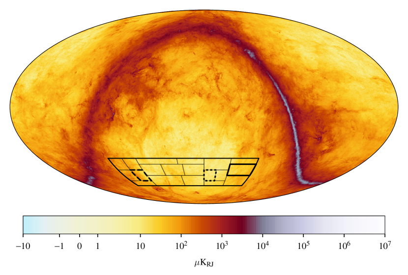
Figure 1: SPT-SZ 2500 deg² footprint and individual field boundaries superimposed on the temperature map of thermal dust from Planck full-mission data (Planck Collaboration et al., 2016d), shown in equatorial coordinates in the Mollweide projection. The two fields with $\simeq\sqrt{2}$ lower than average noise are $(\mathrm{R.A.},\mathrm{dec.})=(5^{\mathrm{h}}30,-55^{\circ})$ (dashed boundary), and $(\mathrm{R.A.},\mathrm{dec.})=(23^{\mathrm{h}}30,-55^{\circ})$ (dotted boundary). The $(\mathrm{R.A.},\mathrm{dec.})=(21^{\mathrm{h}},-50^{\circ})$ field (thick solid boundary) has $\simeq\sqrt{2}$ above average noise for this analysis due to an observation cut (see text for details). The dust map units are Rayleigh-Jeans brightness temperature at a reference frequency of 545.0 GHz.

Maps of the Large and Small Magellanic Clouds using a similar combination of SPT and Planck temperature maps were presented in Crawford et al. (2016). Similarly to Crawford et al. (2016), we use Planck data to fill in the information at large angular scales that is missing from SPT-SZ data and to improve the signal-to-noise at intermediate angular scales where both instruments have high signal-to-noise. Meanwhile the higher-resolution SPT data probes small scales where Planck is dominated by noise. We present three maps of the mm-wave sky combined in this way, namely SPT 95 GHz (3.2 mm) + Planck 100 GHz (3.0 mm), SPT 150 GHz (2.0 mm) + Planck 143 GHz (2.1 mm), and SPT 220 GHz (1.4 mm) + Planck 217 GHz (1.4 mm). Each of these maps cover roughly 2500 deg² of the Southern sky. The wide range of angular scales with high signal-to-noise in these maps makes them useful for a wide array of applications, including CMB lensing measurements (Omori et al., 2017; Simard et al., 2017).

The structure of this paper is as follows. In Section 2 and Section 3 we introduce the SPT and Planck instruments and data. In Sections 4 and 5 we describe the filtering, data processing, and the combining procedure. In Section 6 we show the resulting combined maps and present tests of them. We conclude in Section 7.

2 The South Pole Telescope

The SPT is a 10 m diameter telescope located at the Amundsen-Scott South Pole Station, Antarctica. It was constructed primarily to measure fluctuations in the CMB with high resolution, and for the detection of galaxy clusters through their SZ signatures (Carlstrom et al., 2011). From 2007 to 2011 a region of the southern sky spanning 20^h to 7^h in right ascension (R.A.) and $-65^{\circ}$ to $-40^{\circ}$ in declination (dec.) was observed in three bands centered at 95, 150, and 220 GHz, with resolutions of approximately 1.7, 1.2, and 1.0 arcmin, respectively. This patch of the sky contains relatively low levels of Galactic foreground emission, as shown in comparison to the thermal dust map from Planck data (Planck Collaboration et al., 2016d) in Figure 1. The observations were performed in nineteen sub-regions which together comprise a contiguous 2540 deg² area on the sky (Story et al., 2013, hereafter S13) referred to as the “SPT-SZ survey.”

In this paper we use 95 GHz observations taken between 2009-2011, 150 GHz observations from 2008-2011, and 220 GHz observations from 2008-2011. Two of the fields were observed for roughly twice the average amount of time in the 150 and 220 GHz bands and hence have lower than average noise. These fields are indicated in Figure 1. Roughly half of the $(\mathrm{R.A.},\mathrm{dec.})=(21^{\mathrm{h}},-50^{\circ})$ observations (thick solid outline in Fig. 1) employed a different scanning strategy and are not used here, making this field noisier than average for this analysis. We use the same 2008-2011 observation cuts as Mocanu et al. 2018 (in preparation), except for the 150 GHz $(23^{\mathrm{h}}30,-55^{\circ})$ field, where we use the observation cuts from S13.

3 The Planck Satellite

The Planck satellite completed approximately four and a half surveys of the entire sky (one every six months) between August 2009 and October 2013 (Planck Collaboration et al., 2016a). The Planck High-Frequency Instrument (HFI) observed the sky in six frequency bands centered at 100, 143, 217, 353, 545, and 857 GHz. Maps of the sky in these bands were released in 2013 (Planck Collaboration et al., 2014) and in the 2015 Public Release 2 (PR2; Planck Collaboration et al., 2016a) with greater sensitivity and improved calibration accuracy. We use the PR2 full-mission HFI maps from the 100, 143, and 217 GHz bands, which are those closest in frequency to the SPT-SZ bands (Figure 2b). The resolution of the 100, 143, and 217 GHz Planck maps are approximately 10.0, 7.1, and 5.0 arcmin, respectively.

4 Response Functions and Data Processing

In order to combine SPT data with Planck data we must deconvolve their response functions due to instrument beams and filtering. In this section we describe the model for the total beam-and-filtering response functions. For SPT we describe the steps of filtering and the calculation of the filter transfer functions for each SPT-SZ band. We use the approximation that for each band, a single two-dimensional transfer function describes the filtering over the entire 2500 deg² area. The Planck Collaboration has calculated and published their total response functions, so we only briefly describe them here.

A map of temperature fluctuations on the sphere $\Delta T(\vec{\theta})$ multiplied by a mask $M(\vec{\theta})$ may be decomposed into spherical harmonic coefficients $\tilde{a}_{\ell m}$ using the spherical harmonic transform:

$$\tilde{a}_{\ell m}=\int_{S}\Delta T(\vec{\theta})M(\vec{\theta})Y_{\ell m}(\vec{\theta})\mathrm{d}\Omega,$$ (1)

where the tilde on $\tilde{a}_{\ell m}$ indicates that mode coupling due to the application of the mask has not been corrected for.

The action of a beam response function $B_{\ell m}$ and a filter transfer function $t_{\ell m}$ on the spherical harmonic coefficients of the true temperature map $\tilde{a}_{\ell m}^{\mathrm{in}}$ yields the spherical harmonic coefficients of the observed temperature map $\tilde{a}_{\ell m}^{\mathrm{out}}$. This can be written as

$$\tilde{a}_{\ell m}^{\mathrm{out}}=t_{\ell m}B_{\ell m}\tilde{a}_{\ell m}^{\mathrm{in}}.$$ (2)

Note that $\tilde{a}_{\ell m}^{\mathrm{in}}$ (with the tilde) are the harmonic coefficients of the true full-sky temperature map $a_{\ell m}^{\mathrm{in}}$ (no tilde) after applying the survey mask. From here, the total response function $F_{\ell m}$ is defined:

$$F_{\ell m} \equiv t_{\ell m}B_{\ell m}$$

$$=\frac{\tilde{a}_{\ell m}^{\mathrm{out}}}{\tilde{a}_{\ell m}^{\mathrm{in}}}.$$

4.1 SPT

The beam response of the SPT is well approximated as a circularly symmetric beam $B_{\ell}$, and was estimated with percent-level precision using measurements of planets and bright extragalactic sources, as detailed in, e.g., Schaffer et al. (2011); Keisler et al. (2011). Over the four years of data presented here, the SPT optics were modified slightly, and the observing frequency distribution of detectors in the focal plane changed; as a result, the instrument beams are slightly different for different observing seasons. In this work, we use beams averaged over the four years, with inverse-noise weighting. These year-averaged beams for each band are plotted in Figure 2.

Figure 2: (a) Year-averaged SPT beams for each band (using individual year beams from Keisler et al., 2011). The SPT beams exceed 1.0 because they are normalized to 1.0 at $\ell=750$. Also shown are the Planck beam window functions (which include the beam and filtering) from the Planck Reduced Instrument Model, version 2.00 (Planck Collaboration et al., 2016b) as well as the final beam ($B_{\ell}^{\mathrm{final}}$, in Section 5) we apply to the combined data maps (in blue). (b) Transmission bandpass functions for SPT and the nearest Planck HFI bands, and the derivative of the blackbody spectrum d$B_{\nu}$/d$T$ evaluated at $T_{\mathrm{CMB}}$ overlaid in black.

The filter response of SPT in past analyses has been computed for each individual field and each frequency in flat-sky coordinates. In this analysis, for each band, we combine all of the fields into a contiguous 2500 deg² map, and we compute a two-dimensional transfer function to characterize the filtering of the full 2500 deg² survey. In the following sections we describe these filtering steps and the calculation of the filter transfer functions.

4.1.1 Time Stream Filtering

The SPT was used to observe each field in a series of observations which are composed of successive scans across the sky along azimuth. Adjacent scans are separated by a small step in elevation. As the telescope is located at the South Pole, the scan direction is along R.A., with steps in declination. Time-varying emission from the atmosphere leads to increased noise on large angular scales. The raw time stream data in each scan is filtered to reduce this noise. For more detail on SPT-SZ filtering, see Schaffer et al. (2011).

The time stream data from each scan are fit with a seventh-order polynomial and set of low-order sines and cosines, which are subtracted from these data. This results in an effective scan-direction high-pass filter with a cutoff of $\ell\simeq 270$. Sources measured to be brighter than 50 mJy at 150 GHz are excluded from the fitting (with a 5-arcmin masking radius). Fainter sources are not masked before filtering, which gives them wing-like features (aligned with the scan direction) in the resulting maps.

The six modules of the SPT-SZ camera each contain 160 detectors. Each module is equipped with filters determining their observing frequency (95 GHz, 150 GHz, or 220 GHz). At every time sample and separately for each module, the mean and two spatial gradients of the data from all detectors in a module is subtracted from their data. This reduces atmospheric noise at large angular scales. A low-pass filter is applied in Fourier space to the data from each detector to avoid aliasing when the data are sampled into map pixels.

Note that the transfer function $t_{\ell m}$ as defined in Equation 4 is an approximation when applied to SPT-SZ data, in that the actual filtering is performed on individual scans in the time domain and in Fourier space, which does not transform perfectly into a simple convolution. However, as we will show in Section 6.3.1, this is a very good approximation.

4.1.2 Constructing HEALPix Maps from SPT Fields

We use the “Hierarchical Equal Area isoLatitude Pixelation of a sphere” (HEALPix; Górski et al., 2005) scheme to pixelize our maps. The filtered SPT maps of each field are initially in the Lambert azimuthal equal-area projection. We match the response of each field from the year-varying beams into a common beam in two-dimensional Fourier space. The common beam is chosen to be a $\simeq 2$ arcmin full width at half maximum (FWHM) Gaussian, however this is not the final resolution of the combined maps. This common beam is replaced at the end of the combining pipeline with a 1.85 arcmin FWHM Gaussian.

The fields are beam matched by multiplying the two-dimensional FFT of the co-added temperature map of each field with the ratio of the common beam to the beam for that year and frequency. Then in position space we perform bilinear interpolation of these beam-matched fields onto the nearest HEALPix pixel locations (with resolution $N_{\mathrm{side}}=8192$). We interpolate the weights for each field onto the same HEALPix grid, and compute the weighted sum of the temperature values using these weights. The final combined maps are in HEALPix format with resolution $N_{\mathrm{side}}=8192$.

4.1.3 Masking

We mask the bright sources (flux densities greater than 50.0 mJy at 150 GHz) which are masked during time stream filtering, and regions close to the SPT-SZ boundary. This mask is constructed by cutting holes with radius of 5 arcmin in an SPT-SZ boundary mask. We apodize the mask outside the holes and at the boundary with a Gaussian with $\sigma=5$ arcmin. This mask is applied to SPT and Planck data, noise and simulations.

4.1.4 Calculating the Transfer Functions

The filter transfer functions for each of the 2500 deg² SPT-SZ maps are computed as follows. We create 100 full-sky simulated input maps per band consisting of the lensed CMB, Gaussian foregrounds (which are correlated between bands), and the Poisson-distributed population of point sources with 150 GHz flux densities in the range $6.4~{}\mathrm{mJy}\leq F_{150}\leq 50.0~{}\mathrm{mJy}$ (Everett et al., in preparation). Simulated lensed CMB maps are generated by running LensPix (Lewis, 2005) on temperature power spectra derived from the Planck TT + lowP + lensing cosmology (Planck Collaboration et al., 2016f). We simulate SZ-detected galaxy clusters with statistical significance $\xi\geq 5.0$ in the 150 GHz band from the Bleem et al. (2015) catalog. The clusters are simulated in their observed positions in the 95 GHz and 150 GHz bands (there is negligible SZ signal at 220 GHz). Using the integrated Comptonization $Y_{\mathrm{SZ}}$ (over an 0.75 arcmin radius disk) and core radius $\theta_{c}$ taken from the Bleem et al. (2015) catalogue, the radial temperature profile of each cluster $\Delta T(\theta)$ is computed assuming a projected isothermal $\beta$-model (Cavaliere & Fusco-Femiano, 1976) with $\beta=1$:

$$\Delta T(\theta)=y_{0}T_{\mathrm{CMB}}g_{\nu}(1+\theta^{2}/\theta_{c}^{2})^{\frac{1-3\beta}{2}},$$ (3)

where $y_{0}$ is the peak Compton $y$-parameter, the CMB temperature $T_{\mathrm{CMB}}=2.7255$ K (Fixsen, 2009), $g_{\nu}$ is a function of observing frequency $\nu$, $\theta$ is the angular distance from the cluster center, and $\theta_{c}$ is the cluster core radius (Bleem et al., 2015).

We create 100 simulated maps (one per input sky) for every individual observation of each field at each band. We create mock timestreams from each input map, and these mock timestreams are made into single-observation simulated maps using the same filtering and processing as used on the real data. The individual observation maps of each field at each band are then coadded, and the single-field maps are combined into full 2500 deg² maps in the same way as the real data. This results in 100 simulated 2500 deg² maps in each band; these maps have the same statistical properties as our best estimate of the observed sky.

The input maps and observed maps (in HEALPix format using the method described in Section 4.1.2) are masked, and their spherical harmonic coefficients are computed ($\tilde{a}_{\ell m}^{\mathrm{in}}$ and $\tilde{a}_{\ell m}^{\mathrm{out}}$, respectively). The filter transfer function is then computed by

$$t_{\ell m}\equiv\frac{1}{B_{\ell}}\frac{\left\langle\tilde{a}_{\ell m}^{\mathrm{out}}\left(\tilde{a}_{\ell m}^{\mathrm{in}}\right)^{*}\right\rangle}{\left\langle\tilde{a}_{\ell m}^{\mathrm{in}}\left(\tilde{a}_{\ell m}^{\mathrm{in}}\right)^{*}\right\rangle},$$ (4)

where $\langle...\rangle$ denotes the ensemble average over all simulations, and $B_{\ell}$ is the common beam introduced in Section 4.1.2. Averaging over 100 simulations per band, we compute the transfer function using this equation. The filter transfer functions for each SPT-SZ band are plotted in Figure 3. Applying the property of spherical harmonic coefficients $a_{\ell(-m)}=a_{\ell(+m)}^{*}$ to $t_{\ell m}$, whose imaginary part is negligible, implies $t_{\ell(-m)}=t_{\ell(+m)}$. We therefore only need to plot half of the total number of modes (e.g. $m\geq 0$ or $m\leq 0$). One can interpret $t_{\ell m}$ with $\ell$ on the x-axis and $m$ on the y-axis as follows:

• Larger values of $m$ correspond to smaller angular scales along the SPT scan direction in equatorial coordinates.

• Filtering in the time domain leads to the localized strip of suppressed modes in $t_{\ell m}$ at $m\lesssim 300$.

• Applying a mask with a restricted range of declination and positioned away from the equator (such as the SPT-SZ survey mask) to a full-sky map leads to a triangle-shaped region of suppressed modes at high $m$. This feature is not due to filtering, it is purely from the geometry of the survey mask when viewed in spherical harmonic space. High-$m$ spherical harmonics have most of their power at the equator, so the survey mask suppresses these modes.

• The $\ell$-dependent trend in $t_{\ell m}$ is the smoothing due to the 1 arcmin pixelization, and is the same for all three frequencies. Note that we are showing $t_{\ell m}$ exactly as in Equation 4, so the $\simeq 2$ arcmin beam from beam-matching $B_{\ell}$ is not included.

Figure 3: Two-dimensional filter transfer functions $t_{\ell m}$ of 2500 deg² SPT-SZ data. They are plotted up to $\ell=8000$ to make the $m\lesssim 300$ filtering visible, however in the analysis we have calculated them up to $\ell=16000$. Smaller values of $t_{\ell m}$ indicate more strongly-filtered modes. The common beam from beam-matching the fields is not included in these plots; the suppression of power with increasing $\ell$ is due to the 1 arcmin pixelization. The dark wedge of modes at high $m$ have been set to zero, since these modes have been strongly suppressed due to the mask (see explanation in text) and contribute negligibly to the combined maps. Note that the Planck beam and filter response functions, shown in Figure 2a, are independent of $m$, so there is no need to show them here as well.

4.1.5 Calibration

The units of CMB maps are differential temperature relative to the CMB temperature,

$$\Delta T\equiv T-T_{\mathrm{CMB}},$$ (5)

denoted K_CMB. The calibration accuracy of the Planck maps in the 100, 143, and 217 GHz bands are $\simeq 0.1$ per cent (Table 6 of Planck Collaboration et al., 2016c). We use this highly precise Planck calibration to calibrate the SPT-SZ maps. We use the 150 GHz calibration factor derived from comparison to Planck 143 GHz data in the SPT-SZ footprint from Hou et al. (2018). We then inter-compare the SPT-SZ 95, 150, and 220 GHz maps to obtain calibration factors at 95 and 220 GHz. The uncertainty of these relative calibrations are 0.22, 0.15, and 0.43 percent (in map units) at 95, 150 and 220 GHz respectively.

4.1.6 Beam and Filter Deconvolution

Upon calculating the spherical harmonic coefficients of the SPT data $\tilde{a}_{\ell m}^{\mathrm{SPT}}$ we divide out the filter transfer function $t_{\ell m}$ and the common beam $B_{\ell}$. For the small subset of modes at low $m$ which are heavily suppressed due to filtering in the time domain, the transfer function is close to zero and there is negligible signal. We do not deconvolve $t_{\ell m}$ for modes where $m<300$. These low-$m$ modes get filled in with Planck data later on. The transfer function also becomes exponentially small at high $m$ due to a low-pass filter. This filter is not the reason for the triangle-shaped wedge of modes at high $m$ – that is due to the application of the 2500 deg² survey mask – but it causes the transfer function to fall off at $\ell\simeq 8000$, $m\simeq 5000$. Modes with $m>5000$ remain filtered in the final maps.

4.1.7 Noise Estimation

A half-difference map is calculated for each observation of each field, such that the left-going scans (along increasing R.A.) and right-going scans (along decreasing R.A.) are differenced and divided by 2. This nulls the signal in each scan while preserving the statistics of the noise. The mean of all of the half-difference maps for a field, with a randomly selected half of them multiplied by $-1$, gives us an estimate of the noise in that field. Using random $\pm 1$’s allows us to produce more realizations of the noise. We make 100 noise realizations of each field and each frequency, and construct a HEALPix map out of each of them.

To estimate the two-dimensional noise power $N_{\ell m}$ in each band, we apply the boundary and point-source mask to each noise realization, compute their harmonic transforms $\tilde{n}_{\ell m}$, deconvolve the beam and filter response functions, and then compute their variance:

$$N_{\ell m}=(F_{\ell m})^{-2}\left\langle\left|\tilde{n}_{\ell m}\right|^{2}\right\rangle.$$ (6)

The auto-spectrum of the SPT noise realizations for each frequency, with their beam and filter transfer functions deconvolved, are shown by the dotted lines in Figure 4.

Figure 4: Average auto-spectra of noise realizations of SPT-SZ (dotted), Planck (dot-dashed), and combined SPT-Planck (solid), in comparison with the total expected signal (CMB plus foregrounds in the 2500 deg² patch; the dashed lines). Left panel = 95/100 GHz, middle panel = 150/143 GHz, right panel = 220/217 GHz. The $m<300$ modes were down-weighted with the same filter as the data.

4.2 Planck

The total beam-and-filter response functions $F_{\ell m}$ for the Planck instrument – referred to as “beam window functions” in the Planck literature – have been computed by the Planck Collaboration and are available online through the Planck Legacy Archive. The beam window functions for each Planck band are well-approximated to depend only on $\ell$ (i.e. $F_{\ell m}=F_{\ell}$); they are plotted in Figure 2. The beam window functions do not include the smoothing due to $N_{\mathrm{side}}=2048$ pixelization; we account for this separately.

We use the full-mission Planck HFI maps, which are $N_{\mathrm{side}}=2048$ resolution in Galactic coordinates. We compute the spherical harmonic coefficients of these maps (without any masking) and rotate them to equatorial coordinates using the rotate_alm HEALPix function. We then invert the spherical harmonic transform and mask the resulting maps using the mask from Section 4.1.3. We compute the spherical harmonic transform of the masked Planck maps, divide out the beam window functions, and multiply by the ratio of the $N_{\mathrm{side}}=2048$ to $N_{\mathrm{side}}=8192$ pixel window functions to match the smoothing due to pixelization with the SPT maps.

For each Planck band we use 100 of the “8th Full Focal Plane” noise realizations from the Planck 2015 data release (see Planck Collaboration et al., 2016e) obtained from the Planck Legacy Archive. These are designed to mimic the true noise statistics (including spatial variation) in the full-mission data maps. We repeat the same processing steps as the real data on these Planck noise realizations, then compute the two-dimensional noise power using Equation 6. The auto-spectrum of the Planck noise realizations for each frequency, with their beam and filter transfer functions deconvolved, are the dot-dashed lines in Figure 4.

5 Inverse Noise-power Weighting in 2-D Harmonic Space

The end result of the previous section are the deconvolved spherical harmonic coefficients of SPT $\tilde{a}_{\ell m}^{\mathrm{SPT}}$ and Planck data $\tilde{a}_{\ell m}^{\mathrm{{\sl Planck}}}$ for each SPT and Planck observing band; and estimates of the noise power at each mode for SPT $N_{\ell m}^{\mathrm{SPT}}$ and Planck $N_{\ell m}^{\mathrm{{\sl Planck}}}$, also in each observing band.

The data are combined through a linear weighting in two-dimensional harmonic space

$$\tilde{a}_{\ell m}^{\mathrm{SPT+{\sl Planck}}}=\tilde{a}_{\ell m}^{\mathrm{{\sl Planck}}}W_{\ell m}^{\mathrm{{\sl Planck}}}+\tilde{a}_{\ell m}^{\mathrm{SPT}}W_{\ell m}^{\mathrm{SPT}},$$ (7)

where $W_{\ell m}^{\mathrm{SPT}}$ and $W_{\ell m}^{\mathrm{{\sl Planck}}}$ are the (real-valued) weights. We choose to construct weights which minimize the noise power at each mode in the resulting maps. These weights are given by

$$W_{\ell m}^{\mathrm{SPT}}\equiv\frac{\left(N_{\ell m}^{\mathrm{SPT}}\right)^{-1}}{\left(N_{\ell m}^{\mathrm{SPT}}\right)^{-1}+\left(N_{\ell m}^{\mathrm{{\sl Planck}}}\right)^{-1}},$$ (8)

and

$$W_{\ell m}^{\mathrm{{\sl Planck}}}\equiv\frac{\left(N_{\ell m}^{\mathrm{{\sl Planck}}}\right)^{-1}}{\left(N_{\ell m}^{\mathrm{SPT}}\right)^{-1}+\left(N_{\ell m}^{\mathrm{{\sl Planck}}}\right)^{-1}}.$$ (9)

These weights are shown in Figure 5. One can see that the $\ell$-dependence of the weights (Figure 5) qualitatively agrees with the $\ell$-dependence of the SPT-only and Planck-only noise power spectra in Figure 4; the Planck weights are close to 1.0 at low $\ell$ (where Planck noise is lower than SPT), and close to 0.0 at high $\ell$ (where Planck noise is much greater than SPT), and vice-versa for the SPT weights.

Figure 5: Two-dimensional inverse noise-power weights for (a) SPT (equation 8) and (b) Planck (equation 9). All weights have been multiplied by the filter $M_{\ell m}$ for each band, which is why both SPT and Planck weights are very small at high-$\ell$, low-$m$ (i.e. they do not sum to 1.0 where $M_{\ell m}\neq 1.0$). The dark wedge of modes at high $m$ have been set to zero, since these modes have been strongly suppressed due to the mask and contribute negligibly to the combined maps.

As previously mentioned, the subset of modes at $m\lesssim 300$ are exceptional in that the SPT power has been completely removed by filtering, while the Planck noise power (and hence the combined map noise power at low $m$) increases steeply with $\ell$ (roughly $\sim B_{\ell}^{-2}$) after deconvolving the Planck beam window function $B_{\ell}$. This leads to the total power (signal+noise) per mode $|\tilde{a}_{\ell m}|^{2}$ being up to orders of magnitude greater at low $m$ than at high $m$ for a given $\ell$. In other words, the noise in the combined maps at low $m$ (contributed by Planck) becomes the dominant contribution to the total map power at high $\ell$. This is a problem for the visual appearance of the combined maps, and it negatively affects the stability of the algorithm we use to calculate the inverse spherical harmonic transform (alm2map). We choose to filter this small subset of modes in the combined maps such that at fixed $\ell$, the average power of the low-$m$ modes is approximately equal to the average power of the higher-$m$ modes. We do this by multiplying $\tilde{a}_{\ell m}^{\mathrm{SPT+{\sl Planck}}}$ of the combined data by a filter $M_{\ell m}$ defined to be 1.0 for all $\ell$ and $m$ except the region encompassing $m<300$ for $\ell>600$, where it is set to

$$M_{\ell m}\equiv\left\langle\frac{\sum_{m=350}^{650}|\tilde{a}_{\ell m}^{\mathrm{SPT+{\sl Planck}(sim)}}|^{2}}{\sum_{m=0}^{300}|\tilde{a}_{\ell m}^{\mathrm{SPT+{\sl Planck}(sim)}}|^{2}}\right\rangle_{\mathrm{sims}},$$ (10)

where $\tilde{a}_{\ell m}^{\mathrm{SPT+{\sl Planck}(sim)}}$ are from noisy simulations.

This filter ensures spatially uniform ($m$-independent) signal+noise in the maps. Additionally, we set $M_{\ell m}$ to zero for $m>5000$ modes; above $m\simeq 5000$, the SPT filtering has essentially zeroed out any signal, and we choose not to include these modes in the final maps (as mentioned in Section 4.1.6). The filters for each band are shown in Figure 6. Note that the application of this filter means that the combined maps are not truly unbiased (i.e. having all filters deconvolved), however it improves the visual appearance of the maps by suppressing noisy low-$m$ modes. This filter will be made publicly available, so that users may deconvolve it from the maps and use a different filter if they wish.

Finally, we convolve with a final beam $B_{\ell}^{\mathrm{final}}$, which we choose to be a 1.85 arcmin FWHM Gaussian, and calculate the inverse spherical harmonic transform of $\tilde{a}_{\ell m}^{\mathrm{SPT+{\sl Planck}}}M_{\ell m}B_{\ell}^{\mathrm{final}}$. This gives us the combined data maps. Note that the only smoothing and filtering left in the combined maps is $B_{\ell}^{\mathrm{final}}$, $M_{\ell m}$, and the $N_{\mathrm{side}}=8192$ pixel window function.

Figure 6: The two-dimensional filters $M_{\ell m}$ designed to ensure uniform power (signal+noise) across $m$ at each $\ell$ in the combined data maps. We have zeroed out $m\geq 5000$ because SPT data has been very heavily suppressed (Section 4.1.6). To maintain consistency with previous plots we have zeroed out modes which are heavily suppressed due to the mask (the black region at $m\simeq\ell$.).

6 Results

In this section we present our main result: combined data maps from SPT 95 GHz + Planck 100 GHz, SPT 150 GHz + Planck 143 GHz, and SPT 220 GHz + Planck 217 GHz. We also perform a few tests on the maps.

6.1 Combined Data and Noise Maps

The combined data maps are shown in Figures 7, 8, and 9. The degree-scale structure common to the three maps is primarily the CMB; these large-scale features are contributed by Planck data. The diffuse emission which is brightest closer to the Galactic plane is predominantly thermal dust in the Milky Way. Small-scale foregrounds such as dusty star-forming galaxies and radio sources, the finer-scale structure of the CMB, and the finer-scale structure of Galactic emission, are all contributed mainly by SPT data.

We use the 100 noise simulations for SPT and Planck to make 100 combined SPT-Planck noise simulations for each band. These are processed in the same way as the real combined data. The average angular power spectrum of the noise for each band, which is computed as specified in Section 6.3.1, is plotted in Figure 4.

Figure 7: Temperature map made from combined SPT-SZ 95 GHz and Planck 100 GHz data, plotted in the Lambert azimuthal equal-area projection (top), and zoomed in on an $2^{\circ}\times 4^{\circ}$ patch at (R.A., dec.) = (5.635^∘, -51.883^∘) (bottom). The zoom-ins show SPT-only (far bottom left), Planck-only (left middle), and SPT-Planck (bottom right).

Figure 8: Temperature map made from combined SPT-SZ 150 GHz and Planck 143 GHz data, plotted in the Lambert azimuthal equal-area projection (top), and zoomed in on an $2^{\circ}\times 4^{\circ}$ patch at (R.A., dec.) = (5.635^∘, -51.883^∘) (bottom). The zoom-ins show SPT-only (far bottom left), Planck-only (left middle), and SPT-Planck (bottom right).

Figure 9: Temperature map made from combined SPT-SZ 220 GHz and Planck 217 GHz data, plotted in the Lambert azimuthal equal-area projection (top), and zoomed in on an $2^{\circ}\times 4^{\circ}$ patch at (R.A., dec.) = (5.635^∘, -51.883^∘) (bottom). The zoom-ins show SPT-only (far bottom left), Planck-only (left middle), and SPT-Planck (bottom right).

6.2 Frequency Response of the Combined Maps

As can be seen from Figure 2b, the frequency response functions of the SPT-SZ and Planck data are slightly different. The frequency response of the combined maps thus varies with $\ell$ and $m$, depending on the relative SPT-SZ and Planck weights. Weighted bandpasses for selected values of $\ell$ (at $m=600$) are shown in Figure 10. The most notable $\ell$ dependence in the bandpass functions are at the edges of the bands: the combined frequency response functions have slightly larger bandwidths than SPT or Planck alone. This is unlikely to substantially affect the interpretation of the signal in the combined maps, particularly in the low-foreground SPT-SZ survey region. The modes which are affected by this the most are where the weights are close to 0.5, which occurs where the noise power spectra cross each other in Figure 4. At low and high $\ell$, the combined frequency response is essentially equal to that of Planck and SPT, respectively (except at low-$m$, where it is equal to that of Planck for all $\ell$).

Figure 10: Weighted combination of the SPT-SZ and Planck frequency response functions at various values of $\ell$, such that the resulting curve represents the frequency response in each combined map at each $\ell$. The weights used are those at $m=600$. Note that at $m\lesssim 300$ the frequency response is given by the Planck frequency response, since SPT data is excluded at low values of $m$.

6.3 Tests

The upper halves of Figures 7, 8, and 9 show the 2500 deg² SPT-Planck combined temperature maps. The gain in resolution achieved by combining SPT with Planck data is especially clear in the zoom-ins (the lower halves of Figures 7, 8 and 9). In the following subsections we present tests of the maps using angular power spectra of simulated and real data.

6.3.1 Tests Using Simulated Data

As a test of our algorithm, we have compared the angular power spectrum of simulated combined maps against the input power spectrum. We mentioned in Section 4.1.1 that $t_{\ell m}$ as defined in Equation 4 is an approximation to the true filtering. Now we test this approximation by measuring how accurately we can recover the input power spectra from mock-observed maps after deconvolving $t_{\ell m}$. We also test that the combining algorithm does not bias the power spectrum.

The first part of this test consists of processing simulated noise-free maps in the same way as the real data. Then, using the “Spatially Inhomogeneous Correlation Estimator for Temperature and Polarization” (PolSpice; Chon et al., 2004) code we compute the angular power spectrum of each simulated map $C_{\ell}$, which is usually plotted as $D_{\ell}\equiv\ell(\ell+1)C_{\ell}/2\pi$.

We use the following procedure to correct for the effect of $M_{\ell m}$ on measured power spectra. Using a separate set of simulated maps where the true power spectrum is known ($C_{\ell}^{\mathrm{true}}$), we compute the estimated power spectrum of the simulated maps ($C_{\ell}^{\mathrm{est}}$) after applying the mask to the maps, computing the spherical harmonic transform, applying the filter $M_{\ell m}$, and then inverting the harmonic transform. We compute the ratio of the average biased spectrum to the true spectrum

$$m_{\ell}\equiv\frac{C_{\ell}^{\mathrm{true}}}{\left\langle C_{\ell}^{\mathrm{est}}\right\rangle},$$ (11)

and multiply the estimated power spectrum of the combined maps (simulated and real data) by $m_{\ell}$. We have checked using the separate set of simulated maps that the uncertainty contributed by $m_{\ell}$ is negligible compared to other sources of uncertainty.

Using this procedure we compute auto- and cross-power spectra averaged over a set of 100 simulations. The average power spectra are binned and divided by their corresponding input spectra. These ratios are plotted in Figure 11. A ratio of $1.0$ indicates perfect agreement between the spectra of simulated output and input. For the majority of the $\ell$ range, especially where CMB is the dominant source of fluctuations, the agreement is better than $1$ percent in power. This test shows excess power in the simulations at high values of $\ell$ (most notably $\ell\gtrsim 6000$). The excess power has similar $\ell$ dependence in auto spectra, cross spectra, and across bands. If our calculated transfer functions were noisy we would see excess power in the output simulations. However, we found that the excess power is unaffected by increasing the number of simulations that go into the transfer functions. We also ran this test on each field separately and found that the result does not change significantly from field to field. Together, these findings have led us to believe that the departure from 1.0 at high $\ell$ is likely due to spatial variation in the data weights. We recommend caution when using these maps above $\ell=6000$.

Figure 11: Angular power spectra of simulated noise-free SPT-Planck maps divided by the average angular power spectra of the input maps. The simulated data was processed identically to the real data. On the left we show the auto-spectra relative to the input auto-spectra, and on the right we show the cross-frequency spectra relative to the average cross-frequency spectra of the input maps. A ratio of 1.0 (dotted horizontal line) indicates perfect agreement between the spectra of the simulated maps and the inputs. All of the spectra were binned with bin widths of $\Delta\ell=50$.

6.3.2 Data Power Spectra

We compare auto- and cross-spectra of our SPT-Planck data maps with theoretical power spectra and previously published SPT-SZ power spectra. Specifically, we compare to the power spectra published in S13, which presented the 150 GHz auto-spectrum in the multipole range $650<\ell<3000$, and in George et al. (2015, hereafter G15), which presented auto and cross-spectra of SPT-SZ data in all three bands in the multipole range $2000<\ell<11000$. The theory spectra we compare to are the Planck 2015 best-fit CMB plus best-fit model foreground spectra from G15. These power spectrum comparisons are intended to validate the maps in terms of the transfer functions and noise, not to estimate cosmological parameters.

We note that the target multipole range, and hence the filtering of SPT-SZ data and masking of point sources, in this work is matched to that in S13 and not G15, but we expect to be able to make meaningful comparisons between the two analyses regardless. Sources with 150 GHz flux densities greater than 6.4 mJy were masked in the G15 mapmaking and power spectrum calculations. The maps presented here were made with sources above 50 mJy at 150 GHz masked. For the comparison to G15, we compute auto and cross power spectra using the same 6.4 mJy mask as in that work.

The auto- and cross-spectra are shown in Figures 12 and 13, respectively. The auto-spectra have not had noise bias subtracted; to compare to G15 and S13 spectra (which were computed using individual-observation cross-spectra and hence do not suffer noise bias), we have added the SPT-Planck noise power spectra to the published G15 and S13 auto-spectra and to the theoretical spectra. We have also applied a small correction to the S13 auto-spectrum to account for the different point source mask used in S13. The error bars are the standard deviation of the binned $D_{\ell}$ of noisy simulated maps.

We find that our cross-spectra are in good agreement with the theoretical and G15 cross-spectra. The difference between our observed auto-spectra (signal plus noise) and the expected spectra (theory plus noise spectra, or G15 auto-spectra plus noise spectra) is found to be 3 % of our noise power spectra.

Figure 12: Auto-spectra of the combined SPT-Planck data maps using the 6.4 mJy mask, computed using PolSpice. Theoretical auto-spectra (overlaid in grey) include our best estimate of the statistics of the true sky (CMB + foregrounds). The data auto-spectra are not noise-bias-subtracted. We have added the noise power spectra to the theoretical auto-spectra, the G15 auto-spectra, and the S13 150 GHz auto-spectrum. The S13 auto-spectrum used a 50 mJy point source mask; we have subtracted an estimate of the 6.4 mJy $\leq F_{150}\leq$ 50 mJy point source power from these bandpowers.

Figure 13: Cross-spectra of the combined SPT-Planck data maps using the 6.4 mJy mask, computed using PolSpice. Theoretical cross-spectra (overlaid in grey) include our best estimate of the statistics of the true sky (CMB + foregrounds), including the cross-correlation of foregrounds between bands.

7 Conclusions

We have made maps of the mm-wave southern sky from combined SPT and Planck data in three frequency bands. The three final maps are created with a resolution described by a Gaussian with FWHM of 1.85 arcmin, and individual sources measured to be brighter than 50 mJy at 150 GHz were masked from all three maps. The 150 GHz SPT-SZ map was calibrated to the Planck 143 GHz data in the SPT-SZ patch (Hou et al., 2018). The 95 GHz and 220 GHz SPT-SZ data were calibrated by inter-comparison with the 150 GHz data. We determined the filter response functions of SPT-SZ data, and used previously measured SPT-SZ beam response functions to deconvolve the beam and filter response from 2500 deg² SPT-SZ maps in spherical harmonic space. Estimates of the noise of each instrument were computed and used to combine the SPT and Planck data in spherical harmonic space. A small subset of modes which are relatively noisy in Planck data and are not present in SPT data due to time stream filtering have been suppressed in the final maps so that the signal+noise power is approximately $\ell$-dependent.

The angular power spectra of simulated combined maps is found to agree very well with input power spectra; this test shows a small amount of excess power (percent-level) in the simulated maps above $\ell\simeq 6000$, so we recommend caution when using the maps above this. The auto and cross-power spectra of our combined data maps agree well with theoretical power spectra and previously published SPT-SZ power spectra (Story et al., 2013; George et al., 2015).

Along with the three combined data maps, we provide 5 realizations of the noise in each combined map, and the mask that was applied to all the maps. The maps and mask are in Equatorial coordinates, in HEALPix format with $N_{\mathrm{side}}=8192$ resolution. We provide the two-dimensional filter that was applied to each combined map, as well as a Python script showing how one can apply a different filter to the maps if they wish. All of the data products described in this paper are available at https://pole.uchicago.edu/public/data/chown18/index.html.

References

- Bleem et al. (2015) Bleem, L. E., Stalder, B., de Haan, T., et al. 2015, ApJS, 216, 27
- Carlstrom et al. (2011) Carlstrom, J. E., Ade, P. A. R., Aird, K. A., et al. 2011, PASP, 123, 568
- Cavaliere & Fusco-Femiano (1976) Cavaliere, A., & Fusco-Femiano, R. 1976, A&A, 49, 137
- Chon et al. (2004) Chon, G., Challinor, A., Prunet, S., Hivon, E., & Szapudi, I. 2004, MNRAS, 350, 914
- Crawford et al. (2016) Crawford, T. M., Chown, R., Holder, G., et al. 2016, ApJS, 779, 86
- De Zotti et al. (2010) De Zotti, G., Massardi, M., Negrello, M., & Wall, J. 2010, A&A Rev., 18, 1
- Fixsen (2009) Fixsen, D. J. 2009, ApJ, 707, 916
- George et al. (2015) George, E. M., Reichardt, C. L., Aird, K. A., et al. 2015, ApJ, 799, 177
- Gispert et al. (2000) Gispert, R., Lagache, G., & Puget, J. L. 2000, A&A, 360, 1
- Górski et al. (2005) Górski, K. M., Hivon, E., Banday, A. J., et al. 2005, ApJ, 622, 759
- Hou et al. (2018) Hou, Z., Aylor, K., Benson, B. A., et al. 2018, ApJ, 853, 3
- Keisler et al. (2011) Keisler, R., Reichardt, C. L., Aird, K. A., et al. 2011, ApJ, 743, 28
- Lagache et al. (2005) Lagache, G., Puget, J.-L., & Dole, H. 2005, ARA&A, 43, 727
- Lewis (2005) Lewis, A. 2005, Physical Review D, 71, doi:10.1103/physrevd.71.083008
- Omori et al. (2017) Omori, Y., Chown, R., Simard, G., et al. 2017, ApJ, 849, 124
- Planck Collaboration et al. (2014) Planck Collaboration, Ade, P. A. R., Aghanim, N., et al. 2014, A&A, 571, A1
- Planck Collaboration et al. (2016a) Planck Collaboration, Adam, R., Ade, P. A. R., et al. 2016a, A&A, 594, A1
- Planck Collaboration et al. (2016b) —. 2016b, A&A, 594, A7
- Planck Collaboration et al. (2016c) —. 2016c, A&A, 594, A8
- Planck Collaboration et al. (2016d) —. 2016d, A&A, 594, A10
- Planck Collaboration et al. (2016e) Planck Collaboration, Ade, P. A. R., Aghanim, N., et al. 2016e, A&A, 594, A12
- Planck Collaboration et al. (2016f) —. 2016f, A&A, 594, A13
- Puget et al. (1996) Puget, J.-L., Abergel, A., Bernard, J.-P., et al. 1996, A&A, 308, L5+
- Schaffer et al. (2011) Schaffer, K. K., Crawford, T. M., Aird, K. A., et al. 2011, ApJ, 743, 90
- Simard et al. (2017) Simard, G., Omori, Y., Aylor, K., et al. 2017, ArXiv e-prints, arXiv:1712.07541
- Story et al. (2013) Story, K. T., Reichardt, C. L., Hou, Z., et al. 2013, ApJ, 779, 86
- Sunyaev & Zel’dovich (1980) Sunyaev, R., & Zel’dovich, Y. 1980, ARAA, 18, 537
- Sunyaev & Zel’dovich (1972) Sunyaev, R. A., & Zel’dovich, Y. B. 1972, Comments on Astrophysics and Space Physics, 4, 173