The Uranie platform: an open-source software for optimisation, meta-modelling and uncertainty analysis.

Abstract

The high-performance computing resources and the constant improvement of both numerical simulation accuracy and the experimental measurements with which they are confronted, bring a new compulsory step to strengthen the credence given to the simulation results: uncertainty quantification. This can have different meanings, according to the requested goals (rank uncertainty sources, reduce them, estimate precisely a critical threshold or an optimal working point) and it could request mathematical methods with greater or lesser complexity. This paper introduces the Uranie platform, an open-source framework which is currently developed at the Alternative Energies and Atomic Energy Commission (CEA), in the nuclear energy division, in order to deal with uncertainty propagation, surrogate models, optimisation issues, code calibration…This platform benefits from both its dependencies, but also from personal developments, to offer an efficient data handling model, a C++ and Python interpreter, advanced graphical tools, several parallelisation solutions…These methods are very generic and can then be applied to many kinds of code (as Uranie considers them as black boxes) so to many fields of physics as well. In this paper, the example of thermal exchange between a plate-sheet and a fluid is introduced to show how Uranie can be used to perform a large range of analysis. The code used to produce the figures of this paper can be found in https://sourceforge.net/projects/uranie/ along with the sources of the platform. This paper has been submitted to Computer Physics Communication.

1 Introduction

Uncertainty quantification is the science of quantitative characterisation and reduction of uncertainties in both computational and real world applications. This procedure usually requests a great number of code runs to get reliable results, which has been a real drawback for a long time. In the past few years many interesting developments have been brought to try to overcome this, these improvements coming both from the methodological and computing side. Among the interesting features oftenly used to perform uncertainty quantification, one can state, for instance, sensitivity analysis to get a rough ranking of uncertainty sources and surrogate model generation to emulate the code and perform a complete analysis on it (uncertainty propagation, optimisation, calibration)…Knowing this and with the increasing number of resources available to assess complex computations (fluid evolution with a fine mesh, for instance), physicists should know whether or not it might be useful to increase the mesh resolution. It could instead be more relevant to reduce a specific uncertainty source, or add new locations to be included in a learning database for building a surrogate model.

The Uranie platform has been developed in order to gather the methodological developments coming both from the academic and the industrial world and provide them to the broadest audience possible. This is done, keeping in mind few important aspects such as:

• Open-source: the platform can be used by anyone, and every motivated person can investigate the code and propose improvements or corrections.

• Accessibility: the platform is developed on Linux but a windows-porting is performed. Even though it is written in C++, it can also be used through Python.

• Modularity: the platform is organised in modules so that one should only load requested modules and that analysis can be organised as a compilation of fundamental bricks. The modules are introduced in Figure 1 and discussed later on.

• Genericity: the platform can work on an explicit function but it can also handle a code considering it as a black-box (as long as communications can be done through file, for instance). This assures that Uranie’s methods are non-intrusive and that it can be applied to all science fields.

In this section, the Uranie platform is introduced, from its internal organisation to its dependencies. The physical use-case of this paper, a simplified mono-dimensional thermal exchange model, is later discussed along with a classical strategic plan to tackle uncertainty analysis.

1.1 The Uranie platform

Uranie (the version under discussion here being 3.11.0) is an open-source software dedicated to perform studies on uncertainty, sensitivity analysis, surrogate model generation and calibration, optimisation issues…Developed by the nuclear energy division of the CEA and written in C++, it is based on the ROOT [1] platform (discussed in Section 1.2).

The platform consists in a set of so-called technical libraries, usually referred as modules (represented as the green boxes in Figure 1), each performing a specific task. Some of them are considered low-level, in the sense that they are the foundation bricks upon which rely the rest of the modules, which can be considered more methodologically-oriented (dedicated to a specific kind of analysis).

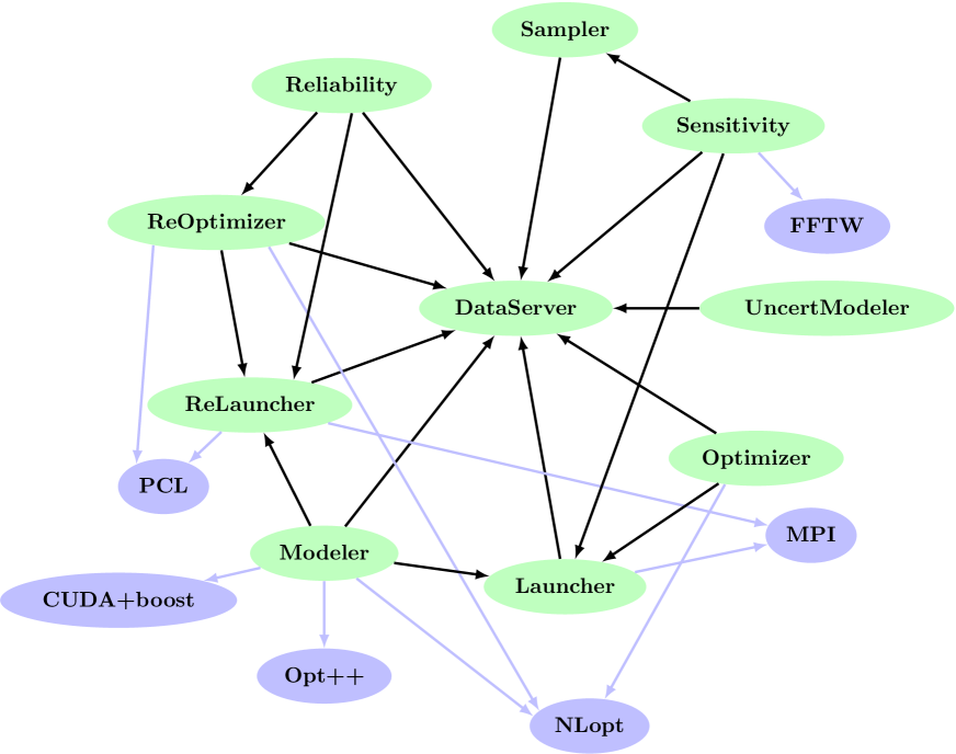
Figure 1: Organisation of the Uranie-modules (green boxes) in terms of inter-dependencies. The external dependencies are shown as light-purple boxes.

In the rest of this section, the main modules, used throughout this paper, will be briefly described (in terms of role) starting with the DataServer one, which is the spine of the Uranie project, as shown in Figure 1.

1.1.1 DataServer module

The DataServer library is the core of the Uranie platform. It contains all the necessary information about the variables of a problem (such as the names, units, probability laws, data files, and so on…), the data itself (if information have been brought or generated) and it allows to perform very basic statistical operations (computing averages, standard deviations, quantiles…).

1.1.2 Sampler module

The Sampler library allows to create a large variety of design-of-experiments depending on the problem to deal with (uncertainty propagation, surrogate model construction, …). Some of these methods are mainly present to be embedded by more complicated methods (such as designs developed in the Fourier-conjugate space, discussed later on in Section 4.3.1).

1.1.3 Modeler module

The Modeler library allows the construction of one or more surrogate models. The idea is to provide a simpler, and hence faster, function to emulate the specified output $Y$ of a complex model (which is generally costly in terms of resources) for a given set of input factors $X_{i}$ (for $i=1,\ldots,n_{X}$, $n_{X}$ being the number of input factors). In this paper, the following surrogate models will be introduced: chaos polynomial expansion, artificial neural network, gaussian process, also known as kriging.

1.1.4 Optimizer and Reoptimizer modules

The Optimizer and Reoptimizer libraries are dedicated to optimisation and model calibration. Model calibration basically consists in setting up the degree-of-freedom of a model such that simulations are as close as possible to an experimental database. The optimisation is a complex procedure and several techniques are available to perform single-criterion or multi-criteria analysis, with and without constraint, using local or global approaches.

1.1.5 Sensitivity module

The Sensitivity library allows to perform sensitivity analysis (SA) of one or several output response $Y$ of a code, with respect to the chosen input factors $X_{i}$ (for $i=1,\ldots,n_{X}$, $n_{X}$ being the number of input factors). A glimpse of the very basic concepts of sensitivity analysis is introduced along with the method used throughout this paper: a screening one (the Morris method) and two different estimation of the Sobol coefficients.

1.2 Uranie installation and external dependencies

Even though the Uranie platform is developed on Linux operating systems, a Windows-version has also been made. In order to check and guarantee the best portability possible, the platform is tested daily on seven different Linux distributions and Windows 7. Getting the source of the Uranie platform can be done at the Sourceforge web page: https://sourceforge.net/projects/uranie/.

Once the sources have been retrieved, it is highly-advised to follow the instruction listed in the README file to perform the installation. On top of the code itself, this installation brings Uranie documentation, among which:

• a methodological manual (both html and pdf format, [2]). It gives a shallow introduction to the main methods and algorithms, from a mathematical point of view, and provides references for the interested reader, to get a deeper insight on these problematics.

• a user manual (both html and pdf format, [3]). It gives explanations on the implementations of methods along with a large number of examples.

• a developer manual. This is a description of methods, from the computing point of view, obtained thanks to the Doxygen platform [4].

In the case of the Windows version, an installation can be done from the previously-introduced archive, but a dedicated free standing archive is specifically-produced by the Uranie support team and is provided on request.

In any case, Uranie has few dependencies to external packages. They are sorted in two categories: the compulsory and optional ones. The latter are shown as light purple boxes in Figure 1 and will only prevent, if not there, some methods from being used. Uranie, on the other hand, can simply not work without the compulsory ones. Both types are listed and briefly discussed below.

1.2.1 Compulsory dependencies

• ROOT: Discussed thoroughly below, the version used here is v5.34/36.

• Cmake: Free and open-source software for managing the build process of compiled software, the version used here is v3.7.1 [5].

• CPPUnit: Unit testing framework for C++ programming, the version used here is v1.13.1 [6].

The ROOT system is an open-source object oriented framework for large scale data analysis. It started as a private project in 1995 at CERN and grew to be the officially supported LHC analysis toolkit. ROOT is written in C++, and contains, among others, an efficient hierarchical object-oriented database, a C++ interpreter, advanced statistical analysis (multi-dimensional histogramming, fitting, minimisation, cluster finding algorithms) and visualisation tools. The user interacts with ROOT via a graphical user interface, the command line or batch scripts. The command and scripting language is C++ (using the interpreter) and large scripts can be compiled and dynamically linked in. The object-oriented database design has been optimised for parallel access (reading as well as writing) by multiple processes.

The ROOT system is developed in C++ (but can be called with other languages such as Python or Ruby though) and is well maintained and documented. Uranie is built as a layer on ROOT and, as a result, it benefits from numerous features of ROOT, among which:

• the C++ interpreter (CINT);

• the Python interface: it provides an automatic transcription of Uranie-classes into Python

• an access to SQL databases;

• many advanced data visualisation features;

• and much more…

1.2.2 Optional dependencies

• OPT++: Libraries that include non linear optimisation algorithms written in C++, the version used here is v2.4 [7]. As this package is not maintained anymore, a patched (and recommended) version is included in the Uranie archive.

• FFTW: Library that computes the discrete Fourier transform (DFT) in one or more dimensions, of arbitrary input size, the version used here is v3.3.4 [8].

• NLopt: Library for nonlinear optimisation, the version used here is v2.2.4 [9].

• PCL: (Portable Coroutine Library) Implements the low level functionality for coroutines, the version used here is v2.2.4.

• MPI: (Message Passing Interface) Standardised and portable message-passing system needed to run parallel computing, the version used here is v1.6.5 [10].

• CUDA: (Compute Unified Device Architecture) Parallel computing platform and programming model invented by NVIDIA to harness the power of the graphics processing unit (GPU), the version used here is v8.0 [11]. If requested, it should be used with the boost library, with a version greater than v1.47.

1.3 The uncertainty general methodology

Many issues related to uncertainty treatment of computer code simulations share the same framework. It can be sketched in a few key steps, gathered for illustration purpose in Figure 2 [12] and described below.

The problem specification (A).

This step is the starting point of a great deal of study as it is when the number of input variable is defined, along with the variable of interest and the corresponding quantity of interest (a quantile, a mean, a standard deviation…). All these are linked through a model that can be a function, a code or even a surrogate model (which can use instead of the code). One can write the general equation that links the model ($f$), the input variables, both uncertain ($\mathbf{x}=(x_{1},\ldots,x_{n_{X}})$) and fixed ($\mathbf{d}=(d_{1},\ldots,d_{n_{D}})$) and the variable of interest $y$, as

$$y=f(\mathbf{x},\mathbf{d})$$ (1)

The quantification of uncertainty source (B).

In this step, the statistical laws followed by the different input variables are chosen along with their characteristics (mean, standard deviation…). The possible correlations between inputs can also be defined here.

The propagation of uncertainty sources (C).

Given the choice made in steps A and B, the uncertainties on the input variables are propagated to get an estimation of the resulting uncertainty on the output under study. This can be performed, for instance, with analytic computation, using Monte-Carlo approach through a design-of-experiments…

The inverse quantification of sources (B’).

Given the definition of the problem in step A and a provided set of experiments, one can measure the mean value and/or the uncertainty of the input variables, in order, for instance, to spot which experiment should be run to constrain the largest one, or to calibrate the model.

The sensitivity analysis (C’).

Given the choice made in steps A and B, this analysis can be used to rank the input variables with respect to the impact of their uncertainty on the uncertainty of the variable of interest. Some methods even provide a quantitative illustration of this impact, for instance as a percentage of the output standard deviation.

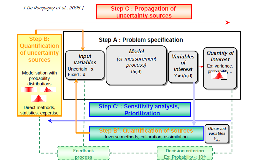
Figure 2: Sketch that represents in few boxes the different steps that can compose an uncertainty propagation or quantification analysis [12].

This is a very broad description of the kind of analysis usually performed when discussing uncertainty quantification. All these steps, can indeed be combined, or replaced, once or in an iterative way, to get a more refined analysis.

1.4 The thermal exchange model

In this part, the physical equations of the use-case used throughout this paper are laid out in a simple way, discussing first the physical equations. This model will be more precisely detailed and also refined as required by the studies performed in the following sections.

1.4.1 Introduction

The experimental setup is depicted in Figure 3 and is composed of a planar sheet whose width is 2$e$ (along the $x$-direction) while its length is considered infinite (represented without boundaries along the $y$-direction). At $t=0$ this sheet, whose initial temperature is set to $T_{i}$, is exposed to a warmer fluid (whose temperature is written as $T_{\infty}$). The aim of this problem is to represent the temperature profiles, depending on the time and the position within the sheet, using different materials for the sheet, and to investigate the impact of various uncertainty sources these temperature profiles.

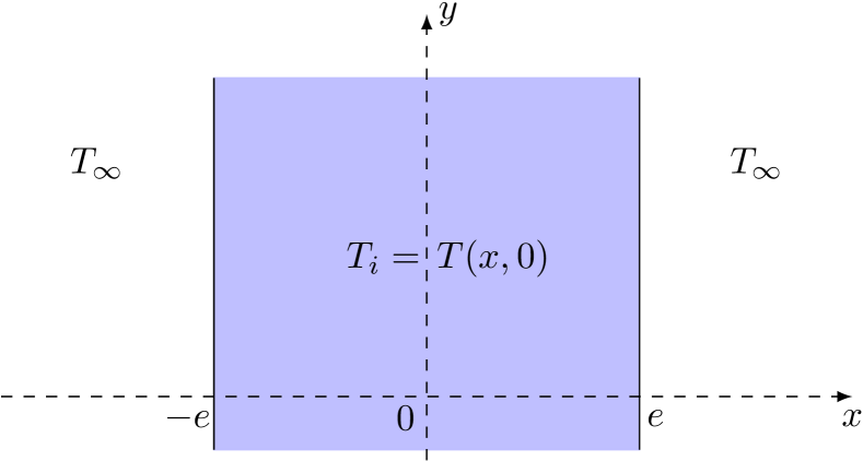
Figure 3: Simplified sketch of the thermal exchange problem

Studying the evolution of the temperature within the sheet in fact consists in solving the heat equation which can be written as follows, if we consider the mono-dimensional problem as depicted in Figure 3:

$$\frac{\partial T}{\partial t}=\alpha\frac{\partial^{2}T}{\partial x^{2}}$$ (2)

In this equation $\alpha$ [m².s^-1] is the thermal diffusivity which is defined by

$$\alpha=\frac{\lambda}{\rho C_{\rho}}$$ (3)

where $\lambda$ is the thermal conductivity [W.m^-1.K^-1], $C_{\rho}$ is the massive thermal capacity [J.kg^-1.K^-1] and $\rho$ is the volumic mass [kg.m^-3]. There are three conditions used to resolve the heat equation, the first one being the initial temperature

$$T(x,t=0)=T_{i}$$ (4)

the second one relies on the flow being null at the centre of the sheet

$$\frac{\partial T}{\partial x}\bigg{|}_{x=0}=0$$ (5)

while the last one relies on the thermal flow equilibrium at the surface of the sheet

$$-\lambda\frac{\partial T}{\partial x}\bigg{|}_{x=e}=h(T(x=e,t)-T_{\infty})$$ (6)

Usually, the thermal coupling between a fluid and a solid structure is characterised by the thermal exchange coefficient h [W.m^-2.K^-1]. This coefficient allows to free oneself from a complete description of the fluid, when one is only interested in the thermal evolution of the structure (and vice-versa). Its value depends on the dimension of the complete system, on the physical properties of both the fluid and the structure, on the liquid flow, on the temperature difference…The thermal exchange coefficient is characterised by the Nusselt number ($N_{u}$), from the fluid point of view, and by the Biot number ($B_{i}$), from the structure point of view. In the rest of this paper, the latter will be discussed and used thanks to the relation

$$B_{i}=\frac{he}{\lambda}$$ (7)

1.4.2 Analytic model

In the specific case where the thermal exchange coefficient, $h$ and the fluid temperature $T_{\infty}$ can be considered constant, Equation (2) has an analytic solution for all initial conditions (all the more so for the one stated in Equation (4)), when it respects the flow conditions defined in Equations (5) and (6). The resulting analytic form is usually express in terms of thermal gauge $\theta$, which is defined as

$$\theta(x,t)=\frac{T(x,t)-T_{i}}{T_{\infty}-T_{i}}$$ (8)

The complete form is the following infinite serie

$$\theta(x_{ds},t_{ds})=2\sum^{\infty}_{n=1}\beta_{n}\cos(\omega_{n}x_{ds})\exp(-\frac{1}{4}\omega^{2}_{n}t_{ds})$$ (9)

where the original parameters have been changed to dimensionless ones

$$x_{ds} = x/e$$ (10)

$$t_{ds} = \frac{t}{t_{D}}=t\times\frac{4\alpha}{e^{2}}=t\times\frac{4\lambda}{e^{2}\rho C_{\rho}}$$ (11)

Given this, the elements in the serie (Equation (9)) can be written

$$\beta_{n}=\frac{\gamma_{n}\sin(\omega_{n})}{\omega_{n}(\gamma_{n}+B_{i})}$$ (12)

where

$$\gamma_{n}=\omega_{n}^{2}+B_{i}^{2}$$ (13)

and $\omega_{n}$ are solutions of the following equation

$$\omega_{n}\tan(\omega_{n})=B_{i}$$ (14)

This model has been implemented in Uranie and tested with two kinds of material to get an idea of the temperature profile in the structure.

1.4.3 Looking at PTFE and iron

In this part, two very different kinds of plate-sheets are compared: a composite one, made out of PTFE (whose best known brand name is Teflon) and an iron one. The main properties (of interest for our problem) of the sheets are gathered in Table 1 side-by-side for both PTFE and iron. The last column shows the relative uncertainty found in the literature (or chosen in the case of the thickness) for the iron case. They will be applied as well on the PTFE. The last three lines are the properties that are computed from the first four ones and once the thermal exchange coefficient has been set to a constant value (here 100), as stated in Section 1.4.2.

	PTFE	Iron		Uncertainty (%)
Thickness [m]: e	10$\times$10-3	20$\times$10-3		0.5
Thermal conductivity [W.m-1.K-1]: $\lambda$	0.25	79.5		0.6
Massive thermal capacity [J.kg-1.K-1]: $C_{\rho}$	1300	444		1.2
Volumic mass [kg.m-3]: $\rho$	2200	7874		0.2
Thermal diffusivity [m2.s-1]: $\alpha$	8.7$\times$10-8	2.27$\times$10-5
Diffusion thermal time [s]: $t_{D}$	287	4.4
Biot number (for $h=100$), [$\varnothing$]: $B_{i}$	4	0.025

Table 1: Summary of both PTFE and iron characteristics. The last column shows the relative uncertainty found in the literature (or chosen in the case of the width) for the iron case. They will be applied as well on the PTFE.

Given these properties, several plots have been produced to characterise the evolution of the temperature profiles in the sheet matter and are gathered in Figure 4. Looking at these plots, a major difference can be drawn between the two sheets: in the PTFE case, the gauge is very different between two positions at a same time and this difference varies also through time (see Figures 4a and 4c). For the iron, on the other hand, the differences through time and space are very small. This is even more important when considering that the range over which the gauge is displayed is significantly reduced. The iron thermal gauge is actually far from reaching the value 1, even after 10 diffusion thermal time, whereas this is the case for PTFE.

(a) $\theta(x_{ds},t_{ds})$ v.s. $x_{ds}$ for PTFE

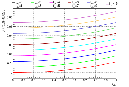
(b) $\theta(x_{ds},t_{ds})$ v.s. $x_{ds}$ for iron

(c) $\theta(x_{ds},t_{ds})$ v.s. $t_{ds}$ for PTFE

(d) $\theta(x_{ds},t_{ds})$ v.s. $t_{ds}$ for iron

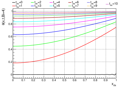
(e) $\theta(x_{ds},t_{ds})$ for PTFE

(f) $\theta(x_{ds},t_{ds})$ for iron

Figure 4: Evolution of the thermal gauge as a function of either the position for different time steps (a,b), the time for different positions (c,d) or depending on both parameters (e,f), for PTFE (left) and iron (right).

These differences could have been foreseen, looking at the properties gathered in Table 1: the previously discussed observations are the expected ones once one considers the value of the Biot number. For a material with a Biot number greater than 1, as the PTFE sheet, the thermal conduction is small within the sheet, leading to temperature gradient within the structure. On the other hand, when the material has a Biot number significantly smaller than 1, as the iron plate, the temperature is expected to be quite similar at the surface and in the centre of the sheet.

1.5 Paper layout

This paper will describe several typical analysis that can be run using the Uranie platform. It is not meant to be fully exhaustive concerning the methodology behind the introduced techniques, but also concerning the methods and options implemented in Uranie. In many cases, though, a sub-part called to go further will introduce briefly the important, yet not discussed, options and solutions that can be offered to the user. Given what has been seen in Figure 4, the use-case used throughout the rest of this paper will be the PTFE case.

The first introduced concept will be the generation of surrogate model (see Section 2). Three different techniques will be applied on an pre-produced design-of-experiments, that will be called the training database, describing the lowest level of complexity of the use-case (only considering the dimensionless variables $x_{ds}$ and $t_{ds}$). A more global picture will be used to take into account the uncertainties introduced in Table 1 and see how to transpose them into uncertainty on the thermal gauge in Section 3. The impact of every uncertainty source will be ranked but also numerically estimated thanks to various sensitivity analysis in Section 4. Finally a calibration of some of the model parameters is performed using different techniques in Section 5, also questioning the fact that the thermal exchange coefficient $h$ can be considered constant. Finally, some important left-over concepts are discussed along with the actual perspectives in Section 6.

2 Surrogate model generation

In this part, different surrogate models will be introduced to reproduce the behaviour of a given code or function. The aim of this step is to obtain a simplified model able to mimic, within a reasonable acceptance margin, the output of both a training and a test database, along with an important improvement in terms of time and memory consumption.

The full analytic model, detailed in Equation (9), plays the role of the complex model that should be approximated. To do so, a training database will be produced, composed of n_S locations (n_S being set to 40 here), written as

$$\mathcal{L}=\{(\mathbf{x}^{j},y^{j}),j=1\ldots n_{S}\}$$ (15)

where $\mathbf{x}^{j}=(x_{ds}^{j},t_{ds}^{j})$ and $y^{j}=\theta(x_{ds}^{j},t_{ds}^{j},B_{i}=4)$. The Biot number is set to 4 as only the PTFE case will be considered (see Table 1).

Three different techniques will be applied: the polynomial chaos expansion, the artificial neural network and the kriging approximation. Each and every method will have a brief introduction before being applied to our use-case. The interested readers are invited to go through the references for a more meticulous description. An example of making practical use of the the kriging surrogate is provided in Section 5. The starting point will always be the loading of the training database in an TDataServer object which is the spine of Uranie.

⬇

//Create the TDataServer object

TDataServer *tds = new TDataServer("tdsObs", "The training DB");

//Load the data in the dataserver

tds->fileDataRead("training_database.dat");

2.1 Polynomial chaos expansion

2.1.1 Introduction

The concept of polynomial chaos development relies on the homogeneous chaos theory introduced by Wiener [13] and further developed by Cameron and Martin [14]. Using polynomial chaos (later referred to as PC) in numerical simulation has been brought back to the light by Ghanem and Spanos [15]. The basic idea is that any square-integrable function can be written as

$$f(\mathbf{x})=\sum_{\alpha}f_{\alpha}\Psi_{\alpha}(\mathbf{x})$$ (16)

where $\{f_{\alpha}\}$ are the PC coefficients, $\{\Psi_{\alpha}\}$ is the orthogonal polynomial-basis. The index over which the sum is done, $\alpha$, corresponds to a multi-index whose dimension is equal to the dimension of the input vector $\mathbf{x}$ (i.e. here $n_{X}$) and whose L1 norm ($|\alpha|_{1}=\sum_{i=1}^{n_{X}}\alpha_{i}$) is the degree of the resulting polynomial.

From this development, it becomes clear that a threshold must be chosen on the order of the polynomials used, as the number of coefficient will growing quickly, following this rule $N_{\rm coeff}=\frac{(n_{X}+p)!}{n_{X}!\,p!}$, where $p$ is the cut-off chosen on the polynomial degree.

2.1.2 Implementation in Uranie and application to the use-case

In Uranie, the implementation of the polynomial chaos expansion method is done through the NISP library ([16]), NISP standing for Non-Intrusive Spectral Projection. Originally written to deal with normal laws, for which the natural orthogonal basis is Hermite polynomials, this decomposition can be applied to few other distributions, using other polynomial orthogonal basis, such as Legendre (for uniform and log-uniform laws), Laguerre (for exponential law), Jacobi (for beta law)…

The PC coefficients are estimated through a regression method, simply based on a least-squares approximation: given the training database $\mathcal{L}$, the vector of output $\mathbf{y}(n_{S})$ is computed with the code. The regression are estimated, given that one calls the correspondence matrix $H(n_{S},p)$ and the coefficient-vector $\boldsymbol{\beta}$, by a minimisation of $||\mathbf{y}-H\boldsymbol{\beta}||^{2}$, where

$$\mathbf{y}=\left(\begin{array}[]{cccc}y^{1}&y^{2}&\ldots&y^{n_{S}}\end{array}\right),$$ (17)

$$H=\left(\begin{array}[]{ccc}\Psi_{1}(\mathbf{x}^{1})&\ldots&\Psi_{p}(\mathbf{x}^{1})\\ \Psi_{1}(\mathbf{x}^{2})&\ldots&\Psi_{p}(\mathbf{x}^{2})\vrule height=11.38092pt,width=0.0pt\\ \vdots&\ddots&\vdots\\ \Psi_{1}(\mathbf{x}^{n_{S}})&\ldots&\Psi_{p}(\mathbf{x}^{n_{S}})\\ \end{array}\right),$$ (18)

$$\boldsymbol{\beta}=\left(\begin{array}[]{c}\beta_{1}\\ \beta_{2}\vrule height=11.38092pt,width=0.0pt\\ \vdots\\ \beta_{p}\end{array}\right)$$ (19)

This leads to write the general form of the solution as $\boldsymbol{\beta}=(H^{T}H)^{-1}H^{T}\mathbf{y}$ which means that the estimation of the points using the surrogate model are given through $\mathbf{\hat{y}}=H\boldsymbol{\beta}=H(H^{T}H)^{-1}H^{T}\mathbf{y}=P\mathbf{y}$, where $P=H(H^{T}H)^{-1}H^{T}$. Here, the P matrix links directly the output variable and its estimation through the surrogate model: this formula is useful as it can be used to compute the Leave-One-Out uncertainty.

Figure 5 represents the distribution of the thermal gauge values (as defined in Equation (8)) estimated by the surrogate model ($\hat{\theta}$) as a function of the ones computed by the complete model ($\theta$) in a validation database containing 2000 locations, not used for the training. A nice agreement is found on the overall range.

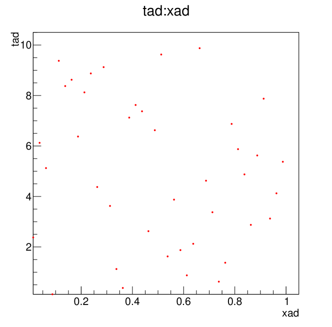
Figure 5: Distribution of the thermal gauge values estimated by the surrogate model ($\hat{\theta}$) as a function of the ones computed by the complete model ($\theta$) in a test database, not used for the training.

In practice, the main steps used to get the PC expansion are gathered in the following block:

⬇

//Create the TNisp object

TNisp *nisp = new TNisp(tds);

//Give sample size (tsize) and method (LHS)

nisp->setSample("Lhs",tsize);

//Create the PC object, given dataserver and nisp object

TPolynomialChaos * pc = new TPolynomialChaos(tds,nisp);

//Set the degree of the PC

pc->setDegree(degree);

//Estimate the coefficient

pc->computeChaosExpansion("Regression");

2.1.3 To go further

There are several points not discussed in this section but which can be of interest for users:

• Based on regression method explained in Section 2.1.2, Uranie also provides a method to estimate the best degree possible, relying on the Leave-One-Out estimation, limiting the range of tested degree, given the learning database size ($n_{S}$).

• PC coefficients can be estimated using an integration methods (instead of the regression) which relies on specific design-of-experiments (usually sparse-grids) that are oftenly smaller, in terms of computations, than the regularly-tensorised approaches  [16].

• When the PC development is done on the natural polynomial basis of the stochastic laws (listed in Section 2.1.2), the PC coefficients can be combined and transformed into Sobol coefficients (discussed in Section 4) providing both a surrogate model and a sensitivity analysis.

2.2 Artificial neural networks

The Artificial Neural Networks (ANN) in Uranie are Multi Layer Perceptron (MLP) with only one hidden layer (containing $n_{H}$ neurons) limited to one output variable ($n_{Y}=1$).

2.2.1 Introduction

The concept of formal neuron has been proposed after observing the way biological neurons are intrinsically connected ([17]). This model is a simplification of the various range of functions dealt by a biological neuron, the formal one (displayed in Figure 6) being requested to satisfy only the two following purposes:

• summing the weighted input values, leading to an output value, called neuron’s activity, $a=\sum^{n_{X}}_{i=i}\omega_{i}x_{i}$, where $\omega_{1},\ldots,\omega_{n_{X}}$ are the synaptic weights of the neuron.

• emitting a signal (whether the output level goes beyond a chosen threshold or not) $s=f(a+\theta)$ where $f$ and $\theta$ are respectively the transfer function and the bias of the neuron.

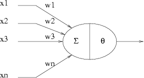
Figure 6: Schematic description of a formal neuron [17].

One can introduce a shadow input defined as $x_{0}=1$ (or -1), which is a way to consider the bias as another synaptic weight $\omega_{0}=\theta$. The resulting emitted signal is written as

$$s=f(\sum^{n_{X}}_{i=0}\omega_{i}x_{i})$$

There are a large variety of transfer functions possible, and an usual starting point is the sigmoid family, defined with three real parameters, c, r and k, as $f_{c,k,r}(x)=c\frac{e^{kx}-1}{e^{kx}+1}+r$. Setting these parameters to peculiar values leads to known functions such as the hyperbolic tangent and the logistic function, shown in Figure 7 and defined as

$$f_{1,2,0}(x)=\frac{e^{2x}-1}{e^{2x}+1}=\frac{e^{x}-e^{-x}}{e^{x}+e^{-x}}=\tanh(x)$$

and

$$f_{1/2,1,1/2}(x)=\frac{1}{2}\frac{e^{x}-1}{e^{x}+1}+\frac{1}{2}=\frac{1}{1+e^{-x}}$$

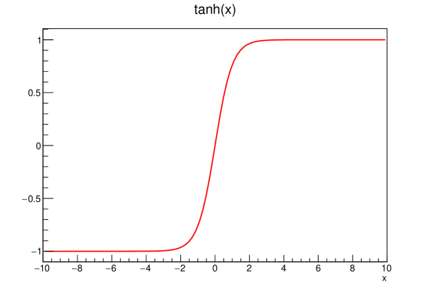
(a) tanh

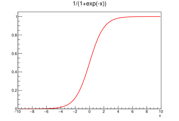
(b) logistic

Figure 7: Example of transfer functions: the hyperbolic tangent (left) and the logistical one (right).

The first artificial neural network conception has been proposed and called the perceptron [18]. The architecture of a neural network is the description of the organisation of the formal neurons and the way they are connected together. There are two main topologies:

• complete: all the neurons are connected to the others.

• by layer: neurons on a layer are connected to all those on the previous and following layer.

2.2.2 Implementation in Uranie and application to the use-case

The general organisation of Uranie’s ANN is detailed in three steps in the following part and displayed in Figure 8. The first layer, where the vector of entries is stored, is called the input layer. The last one, on the other hand, is called the output layer while in between lies the single hidden layer, composed of $n_{H}$ hidden neurons.

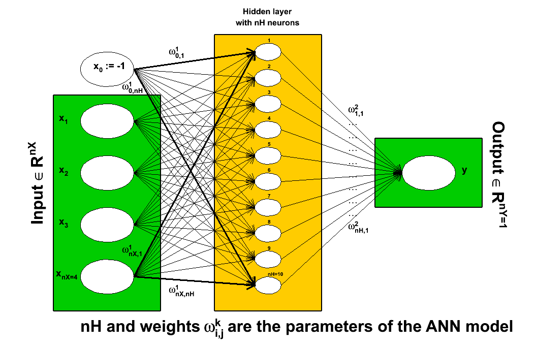
Figure 8: Schematic description of the working flow of an ANN as used in Uranie.

The first step is the definition of the problem: what are the input variables under study, how many neurons will be created in the hidden layer, what is the chosen activation function.

The second step is the training of the ANN. Using the full database $\mathcal{L}$, two mechanisms are run simultaneously:

• the learning itself. By varying all the synaptic weights contained in the parameter $\Xi$, the aim is to produce the output set $\hat{y}=f_{\Xi}(\mathbf{x})$, that would be as close as possible to the output stored in $\mathcal{L}$ then keep the best configuration (denoted as $\Xi^{*}$). The difference between the real output and the estimated one is measured through a loss function which could be, in the case of regression, a quadratic loss function such as

  $$L(y,\hat{y})=\frac{1}{2}||y-\hat{y}||^{2}$$

  From there, one can define the risk function $R(\Xi)$ used to transform the optimal parameters search into a minimisation problem. The empirical risk function can indeed be written as

  $$R(\Xi)=\frac{1}{n_{S}}\sum^{n_{S}}_{i=1}L(y_{i},f_{\Xi}(\mathbf{x_{i}}))$$

• the regularisation. Since the ANN is trained only on the $\mathcal{L}$ ensemble, the surrogate model could be trained too specifically for this sub-part of the input space which might not be representative of the overall input space. To avoid this, the learning database is split into two sub-parts: one for the training (see previous bullet), and one to prevent the over-fitting to happen. For every newly tested parameter set $\Xi$, the generalised error (computed as the average error over the set of points not used in the training procedure) is determined. While it is expected that the risk function is becoming smaller when the number of optimisation steps is getting higher, the generalised error is also becoming smaller at first, but then it should stabilise and even get worse. This flattening or worsening is used to stop the optimisation.

This procedure is stochastic: the splitting of the $\mathcal{L}$ ensemble is done using a random generator, so does the initialisation of the synaptic weights for all the formal neurons. It is important then to export the constructed neural network as running twice the same methods will not give the same performances.

Figure 9 represents the distribution of the thermal gauge values (as defined in Equation (8)) estimated by the surrogate model ($\hat{\theta}$) as a function of the ones computed by the complete model ($\theta$) in a test database containing 2000 points, not used for the training. A nice agreement is found on the overall range.

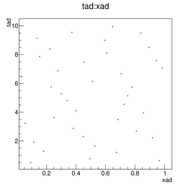
Figure 9: Distribution of the thermal gauge values estimated by the surrogate model ($\hat{\theta}$) as a function of the ones computed by the complete model ($\theta$) in a test database, not used for the training.

In practice, the main steps used to get the neural network trained are gathered in the following block:

⬇

//Create ANN object, providing dataserver and its architecture (the inputs, the number of neurons and the output)

TANNModeler* tann = new TANNModeler(tds, Form("xad:tad,\%d,theta", nH));

//Define the activation function

tann->setNormalization(TANNModeler::kMinusOneOne);

//Train the ANN (5 learning/regularisation splitting and 10 weight initialisation)

tann->train(5, 10,);

2.2.3 To go further

There are several points not discussed in this section but which can be of interest for users:

• The learning step can be run in parallel on graphics processing units (GPU) which can boost it considerably.

• Even though this surrogate model is not yet implemented for several outputs, one can create an ANN which embeds the results of other neural networks.

Several investigations are ongoing to improve this technique, among which:

• Implement a multi-output approach

• Implement a multi-hidden layers approach

• Use Hamiltonian Markov Chain for the synaptic weight [19]

2.3 Kriging

First developed for geostatistic needs, the kriging method, named after D. Krige and also called Gaussian Process method (denoted GP hereafter) is another way to construct a surrogate model. It recently became popular thanks to a series of interesting features:

• it provides a prediction along with its uncertainty, which can then be used to plan simulations and therefore improve predictions of the surrogate model

• it relies on relatively simple mathematical principle

• some of its hyper-parameters can be estimated in a Bayesian fashion to take into account a priori knowledge.

Kriging is a family of interpolation methods developed for the mining industry [20]. It uses information about the ”spatial” correlation between observations to make predictions along with a confidence interval at new locations. In order to produce the prediction model, the main task is to produce a spatial correlation model. This is done by choosing a correlation function and search for its optimal set of parameters, based on a specific criterion.

2.3.1 Introduction

The modelisation relies on the assumption that the deterministic output $y(\mathbf{x})$ can be written as a realisation of a gaussian process $Y(\mathbf{x})$ that can be decomposed as $Y(\mathbf{x})=m(\mathbf{x})+Z(\mathbf{x})$ where $m(\mathbf{x})$ is the deterministic part, called hereafter deterministic trend, that describes the expectation of the process and $Z(\mathbf{x})$ is the stochastic part that allows the interpolation. This method can also take into account the uncertainty coming from the measurements. In this case, the previously-written $Y(\mathbf{x})$ is referred to as $Y_{\rm Real}(\mathbf{x})$ and the gaussian process is then decomposed into $Y_{\rm Obs}(\mathbf{x})=m(\mathbf{x})+Z(\mathbf{x})+\epsilon(\mathbf{x})$, where $\epsilon(\mathbf{x})$ is the uncertainty introduced by the measurement.

To construct the model from the training database $\mathcal{L}$, a parametric correlation function can be chosen along with a deterministic trend (to bring more information on the behaviour of the output expectation). These steps define the list of hyper-parameters to be estimated ($\Xi$) by the training procedure. The best estimated hyper-parameters ($\Xi^{*}$) constitute then the kriging model that can then be used to predict the value of new points.

To end this introduction, it might be useful to show a very-general correlation function: the Matern function, called hereafter $K_{\nu}$. It uses the Gamma function $\Gamma$ and the modified Bessel function of order $\nu$. This $\nu$ parameter describes the regularity (or smoothness) of the trajectory (the larger, the smoother) which should be greater than 0.5. In one dimension, with $\delta x$ the distance, this function can be written as

$$c(\delta x)=\frac{1}{\Gamma(\nu)2^{\nu-1}}\left(2\sqrt{\nu}\frac{\delta x}{l}\right)^{\nu}K_{\nu}\left(2\sqrt{\nu}\frac{\delta x}{l}\right).$$ (20)

In this function, $l$ is the correlation length parameter, which has to be positive. The larger $l$ is, the more $Y$ is correlated between two fixed locations $x_{1}$ and $x_{2}$ and hence, the more the trajectories of $Y$ vary slowly with respect to $x$.

2.3.2 Implementation in Uranie and application to the use-case

The kriging approximation in Uranie is provided through the gpLib library [21]. Based on the gaussian process properties of the kriging [22], this library can estimate the hyper-parameters of the chosen correlation function in several possible ways, then build the prediction model. More details about these steps are provided hereafter and in the gpLib tutorial [23].

The first step is to construct the model from a training database $\mathcal{L}$, by choosing a parametric correlation function, amongst the list below, for which $l$ is the vector of correlation lengths and $\nu$ is the vector of regularity parameters:

• Gauss: defined with one parameter per dimension, as $c(\delta\mathbf{x})=\exp\left[-\sum_{k=1}^{n_{X}}\left(\frac{\delta x_{k}}{l_{k}}\right)^{2}\right]$.

• Isogauss: defined with one parameter only, as $c(\delta\mathbf{x})=\exp\left[-\frac{|\delta\mathbf{x}|^{2}}{l^{2}}\right]$.

• Exponential: defined with two parameters per dimension, as $c(\delta\mathbf{x})=\exp\left[-\sum_{k=1}^{n_{X}}\left(\frac{|\delta x_{k}|}{l_{k}}\right)^{p_{k}}\right]$, where $p$ are the power parameters. If $p=2$, the function is equivalent to the Gaussian correlation function.

• MaternI: the most general form, defined with two parameters per dimension, as $c(\delta\mathbf{x})=\prod_{k=1}^{n_{X}}\frac{1}{\Gamma(\nu_{k})2^{\nu_{k}-1}}\left(2\sqrt{\nu_{k}}\frac{\delta x_{k}}{l_{k}}\right)^{\nu_{k}}K_{\nu_{k}}\left(2\sqrt{\nu_{k}}\frac{\delta x_{k}}{l_{k}}\right).$

• MaternII: defined as maternI, with only one smoothness (leading to $n_{X}+1$ parameters).

• MaternIII: the distance $\boldsymbol{\delta}=\sqrt{\sum_{k=1}^{n_{X}}\left(\frac{\delta x_{k}}{l_{k}}\right)^{2}}$ is put in Equation (20) instead of $\delta x$ (leading to $n_{X}+1$ parameters).

• Matern3/2: equivalent to maternIII, when $\nu=3/2$.

• Matern5/2: equivalent to maternIII, when $\nu=5/2$.

• Matern7/2: equivalent to maternIII, when $\nu=7/2$.

The next step is to find the optimal hyper-parameters ($\Xi^{*}$) of the correlation function and the deterministic trend (if one is prescribed), which can be done in Uranie by choosing:

• an optimisation criterion (in the example: the log-likelihood function);

• the size of the design-of-experiments used to define the best starting point for the optimisation;

• an optimisation algorithm configured with a maximum number of runs;

Once the “best” starting point is found, the chosen optimisation algorithm is used to seek for an optimal solution. Depending on various conditions, convergence can be difficult to achieve. Once done, the kriging surrogate model can be applied to the testing database to get predicted output values and their corresponding uncertainties.

It is, however, possible, even before using a testing database, to check the specified covariance function at hand, using the Leave-One-Out technique (Loo). This method consists in the prediction of a value for $y_{i}$ using the rest of the known values in the training site, i.e. $y_{1},\,\ldots,\,y_{i-1},\,y_{i+1},\,\ldots,\,y_{n_{S}}$ for $i=1,\ldots,n_{S}$. From there, it is possible to use the Leave-One-Out prediction vector $(y^{Loo}_{i})_{i=1,\,\ldots,\,n_{S}}$ and the expectation $\bar{y}$ to calculate two criteria: the Mean Square Error (MSE) and the quality criteria $Q^{2}_{Loo}$ defined as

$$MSE_{Loo}=\frac{1}{n_{S}}\sum_{i=1}^{n_{S}}(y_{i}-y^{Loo}_{i})^{2}$$

and

$$Q^{2}_{Loo}=1-\sum_{i=1}^{n_{S}}\frac{(y_{i}-y^{Loo}_{i})^{2}}{(y_{i}-\bar{y})^{2}}.$$

The first criterion should be close to 0 while, if the covariance function is correctly specified, the second one should be close to 1. Another possible test to check whether the model seems reasonnable consists in using the predictive variance vector $(\sigma^{2}_{y^{Loo}_{i}})_{i=1,\,\ldots,\,n_{S}}$ to look at the distribution of the ratio $(y_{i}-y^{Loo}_{i})^{2}/\sigma^{2}_{y^{Loo}_{i}}$ for every point in the training site. A good modelling should result in a standard normal distribution.

The kriging technique has been applied twice to illustrate its principle and the results are gathered in Figure 10. In the first case, it is used on a mono-dimensional thermal gauge evolution as a function of the dimensionless time, see Figure 10a. On this figure, the black points represent the training database while the blue and red ones are respectively the real output values and their estimated counterpart from the kriging model using the testing database. A good agreement is found and confirmed by the MSE and $Q^{2}$ criteria. The red band represents the uncertainty on the estimation. The kriging approximation has also been applied to $\mathcal{L}$, as for the ANN and PC, and a nice agreement is found on the overall range, as shown in Figure 10b.

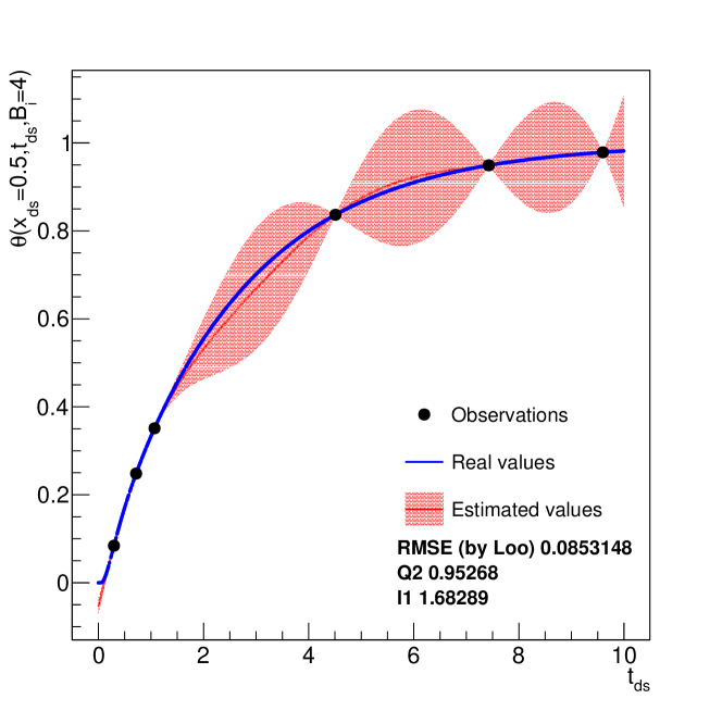
(a) $\theta(x_{ds}=0.5,t_{ds},B_{i}=4)$ and the kriging model

(b) $\hat{\theta}$ vs. $\theta$

Figure 10: Distribution of the thermal gauge values, in a test database, computed with the code (in blue) and estimated by a kriging model (in red) whose training database is shown as black points (a). Distribution of the thermal gauge values estimated by the surrogate model ($\hat{\theta}$) as a function of the ones computed by the complete model ($\theta$) in a test database, not used for the training (b).

In practice, the main steps used to get the kriging model gathered in the following block:

⬇

//Create the GPBuilder object (given a dataserver, inputs, output, correlation function and a trend)

TGPBuilder *gpb = new TGPBuilder(tds,"xad:tad","theta","matern5/2","linear");

//Find best hyper-parameters (with Subplexe algorithm with ML criterion

gpb->findOptimalParameters("ML", 1000, "Subplexe", 1000);

//Construction of the Kriging object

TKriging *kg = gpb->buildGP();

2.3.3 To go further

There are several points not discussed in this section but which can be of interest for users:

• other optimisation criteria. Thanks to the linear nature of the kriging model, the Leave-One-Out error has an analytic formulation [21];

• on top of the deterministic trend, an a priori knowledge on the mean and variance of the trend parameters can be used to perform a Bayesian study;

• one can take into account measurement errors when looking for the optimal hyper-parameters;

On top of the already introduced surrogate models, Uranie can provide few other solutions among which:

• the regression method;

• the k-nearest neighbour method;

• the kernel method.

3 Uncertainty propagation

As already stated in Section 1.3, many analysis will start in the same way, by defining the problem investigated in terms of number of input variables and their characteristics, setting their possible correlations…From there, unless one has an already computed set of experiments (as it was the case in Section 2), it is common to generate a design-of-experiments as being a set of input locations to be assessed by the code/function and that should be the most representative of the input phase space with respect to aim of the study.

This section introduces the various mechanisms available in Uranie for sampling design-of-experiments, which could lead to the uncertainty propagation from the input parameters to the quantity of interest, as shown in Figure 2.

3.1 Random variable definition

3.1.1 Defining a variable

Uranie implements more than fifteen parametric distributions (continuous ones) to describe the behaviour of a given random variable. The list of available continuous laws is given in Table 2, along with their corresponding adjustable parameters. For a complete description of these laws and a set of variations of all these parameters, see [2]. The classes, implementing these laws, give access to the main mathematical properties (theoretical ones) and they have been made to be an interface with the sampling methods discussed in Section 3.2, to get a dedicated design-of-experiments.

Law	Adjustable parameters
Uniform	Min, Max
Log-uniform	Min, Max
Triangular	Min, Max, Mode
Log-triangular	Min, Max, Mode
Normal (gaussian)	Mean, Sigma
Log-normal	Mean, Sigma
Trapezium	Min, Max, Low, Up
Uniform by parts	Min, Max, Median
Exponential	Rate, Min
Cauchy	Scale, Median
GumbelMax	Mode, Scale
Weibull	Scale, Shape, Min
Beta	alpha, beta, Min, Max
GenPareto	Location, Scale, Shape
Gamma	Shape, Scale, Location
Inverse gamma	Shape, Scale, Location

Table 2: List of continuous available statistical laws in Uranie, along with their corresponding adjustable parameters.

These classes offer also methods to compute the probability density function (PDF), the cumulative distribution function (CDF) and its inverse-CDF. Figure 11 shows example of PDF distributions in Figure 11a, CDF distributions in Figure 11b and inverse-CDF distribution in Figure 11c, using an uniform (black), a normal (red) and a gumbelmax (blue) law.

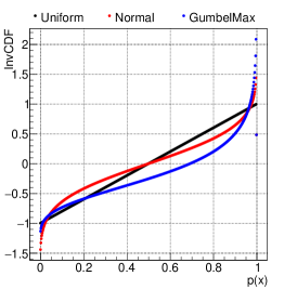
(a) PDF

(b) CDF

(c) inverse-CDF

Figure 11: Example of PDF (a), CDF (b) and inverse-CDF (c) for an uniform law (defined between -1 and 1, in black), a normal law (with $\mu=0$ and $\sigma=0.5$, in red) and a gumbelmax one (with $\mu=-0.4$ and $\beta=0.4$ in blue).

On top of these definitions, it is also possible to create a new variable through a combination of already existing ones, for instance with simple mathematical expression. This can be done independently of the origin of the original variables: either read from a set-of-experiments without any knowledge of the underlying law, or generated from well-defined stochastic law.

3.1.2 Correlating the laws

Once the laws have been defined, one can introduce correlation between them. This, in Uranie, can be done with different methods. Starting from the simplest one, one can introduce a correlation coefficient between two variables or providing the complete correlation matrix.

Instead of using correlation matrix to get intricated variables, one can use methods relying on copula, in order to describe the dependencies. The idea of a copula is to define the interaction of variables using a parametric function that can allow a broader range of entanglement than only using a correlation matrix (various shapes can be done). The copulas provided in the Uranie platform are archimedian ones, with 4 pre-defined parametrisation: Ali-Mikhail-Haq, Clayton, Frank and Plackett.

Both methods will be illustrated in the next section.

3.2 Design-of-experiments definition

3.2.1 Stochastic methods

In Uranie, different kind of random-based algorithms can be used to generate design-of-experiments. Here is a brief introduction of the three main types which are illustrated in Figure 12 where two independent uniformly-distributed variables are used. This kind of plot (called Tufte one) is an example of Uranie-implemented visualisation tool. The main pad, in the centre of the canvas, shows the dependence of the two variables under consideration, while the two other pads show projection along one of the dimension, as a mono-dimensional histogram.

Simple Random Sampling (SRS):

This method consists in independently generating the samples for each parameter following its own probability density function. An example of this sampling when having two independent uniformly-distributed variables is shown in Figure 12b. The random drawing is performed using an uniform law between 0 and 1 and getting the corresponding value by calling the inverse CDF function corresponding to the law under study.

Latin Hypercube Sampling (LHS):

This method [24] consists in partitioning the variation interval of each variable to obtain equiprobable segments and then get, for each segment, a representative value. An example of this sampling when having two independent uniformly-distributed variables is shown in Figure 12a. The random drawing is performed using an uniform law between 0 and 1, split into the requested number of points for the design-of-experiments. Thanks to this, a grid is prepared, assuring equi-probability in every axis-projection. Finally, a random drawing is performed in every sub-range. The obtained value is computed by means of the inverse CDF function corresponding to the law under study.

maximin LHS:

Considering the definition of a LHS sampling, it is clear that permuting a coordinate of two different points creates a different design-of-experiments that is still a LHS one. In Uranie, a new kind of LHS sampling, called maximin LHS, has been recently introduced with the purpose of maximising the minimal distance calculated between every pair of two design locations [25]. The criterion under consideration is the mindist criterion: let $D=[\mathbf{x}_{1},\cdots,\mathbf{x}_{n_{S}}]\subset[0,1]^{n_{X}}$ be a design-of-experiments, made out of $n_{S}$ points. It is written as

$$\min_{i,j}{||\mathbf{x}_{i}-\mathbf{x}_{j}||_{2}}$$ (21)

where $||.||_{2}$ is the euclidean norm. The designs which maximise the mindist criterion are referred to as maximin LHS. It has been observed that the best designs in terms of maximising Equation (21) can be constructed by minimising its $L^{p}$ regularisation instead, $\phi_{p}$, which can be written:

$$\phi_{p}:=\Big{[}\sum_{i<j}||\mathbf{x}_{i}-\mathbf{x}_{j}||_{2}^{p}\Big{]}^{\frac{1}{p}}.$$ (22)

The permutations done to go from a first LHS design-of-experiments to its maximin version are made through a simulated annealing method. An example is displayed, starting from the design-of-experiments in Figure 12a and resulting in the one in Figure 12c. Both have uniform projections along each axis but the locations are clearly more space-filling in Figure 12c.

(a) LHS drawing

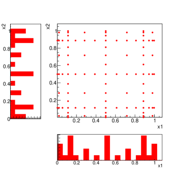
(b) SRS drawing

(c) maximin LHS drawing

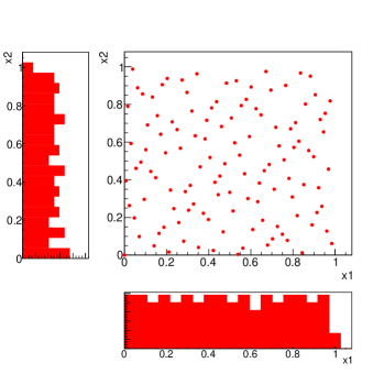
(d) Halton sequence

(e) Sobol sequence

(f) Petras algorithm

Figure 12: Drawing of the design-of-experiments for two uniformly-distributed variable $x1$ and $x2$, with a LHS sampling (a), a SRS one (b) and a maximin LHS one (c). Deterministic sampling are shown also with the Halton sequence (d), the Sobol one (e) and a Petras sparse grid (f).

The SRS method is a pure-random method which populates the region following the inverse-CDF of the considered probability law. In other words, if the objective is to obtain quantiles for extreme probability values, the size of the sample should be large for this method to be used. However, one should keep in mind that it is rather trivial to double the size of an existing SRS sampling, as no extra caution has to be taken apart from the random seed. On the other hand, the LHS method is built in a way that ensure that the domain of variation of each variable is totally covered in a homogeneous way. The drawback of this construction is that it is absolutely not possible to remove or add points to a LHS sampling without having to regenerate it completely.

From a theoretical perspective, using a maximin LHS to build a GP emulator can reduce the predictive variance when the distribution of the GP is exactly known. However, it is not often the case in real applications where both the variance and the range parameters of the GP are actually estimated from a set of learning simulations run over the maximin LHS. Unfortunately, the locations of maximin LHS are far from each other, which is not a good feature to estimate these parameters with precision. That is why maximin LHS should be used with care. Relevant discussions dealing with this issue can be found in [26].

Finally, as introduced in Section 3.1.2, an example of correlation is provided in Figure 13, both using correlation coefficient and copula. In the first case, instead of relying on the “Bravais-Pearson” correlation coefficient definition, that exclusively reflects both the degree and sign of linearity between two variables $x_{i}$ and $x_{j}$ , the method used in Uranie [27] takes into account the correlation on ranks, i.e. the “Spearman” definition:

$$\rho^{S}(x_{i},x_{j})=\rho(R_{x_{i}},R_{x_{j}})=\frac{{\rm Cov}(R_{x_{i}},R_{x_{j}})}{\sqrt{{\rm Var}(R_{x_{i}}){\rm Var}(R_{x_{j}})}}$$ (23)

In this expression, $\rho^{S}$ is the Spearman coefficient, $\rho$ is the usual Bravais-Pearson definition but applied here on $R$ which is the rank of the information under consideration. This method can be applied only if the correlation matrix provided by the user is positive definite. Figure 13a shows an example of correlation (set to a value of 0.9) between two uniform distributions.

The copula, introduced in Section 3.1.2 depend only on the input variables and a parameter $\xi$. An example using two uniform distributions is given in Figure 13b for the Ali-Mikhail-Haq copula.

(a) Spearman coefficient

(b) Ali-Mikhail-Haq Copula

Figure 13: Example of correlation introduced between two uniform distributions, using either the Spearman coefficient (a) or a Ali-Mikhail-Haq copula (b).

3.2.2 Quasi Monte-Carlo methods

The deterministic samplings can produce design-of-experiments with specific properties, that can be very useful in cases such as:

• cover at best the space of the input variables

• explore the extreme cases

• study combined or non-linearity effects

There are two kinds of quasi Monte-Carlo sampling methods implemented in Uranie: the regular ones and the sparse grid ones. The former can be generated using two different sequences:

1. Sequences of Halton [28]

2. Sequences of Sobol [29]

Figures 12d and 12e show the design-of-experiments obtained when having two independent uniformly-distributed variables and can be compared with the stochastic ones (from Figure 12a to Figure 12c) already discussed in Section 3.2.1. The coverage is clearly more regular in the case of quasi Monte-Carlo sequences, but these methods can suffer from weird pattern appearance when $n_{X}$ is greater than 10. On the other hand, the sparse grid sampling can be very useful for integration purposes and can be used in some of the meta-modelling definition, see, for instance, in Section 2.1.3. In Uranie, the Petras algorithm [30] can be used to produce these sparse grids, (shown when the level is set to 8, in Figure 12f, that can be compared to the rest of of the design-of-experiments in Figure 12.

In practice, the main steps used to get one of the plot shown in the Figure 12 are gathered in the following block:

⬇

//Creation of the dataserver

TDataServer *tds = new TDataServer("tds","the dataserver");

//Definition of two uniform variables, with a name, min and max value

tds->addAttribute( new TUniformDistribution("x1",0,1) );

tds->addAttribute( new TUniformDistribution("x2",0,1) );

//Define the sampling (given the dataserver, the method to be used and the number of locations)

TSampling *sam = new TSampling(tds,"srs",size);

//Generation of the samples

sam->generateSample();

//Draw the design-of-experiments (Uranie method)

tds->drawTufte("x2:x1");

3.2.3 To go further

This introduction to the design-of-experiments sampling is very brief with respect to the underlying complexity and possibility. It is indeed also possible to produce with Uranie:

• design-of-experiments for integration in the conjugate Fourier space;

• a representative set-of-points smaller than a given database to keep the main behaviour without having to run too many computations;

3.3 Focusing on the PTFE case

In this section, the basic building blocks introduced in Section 3.1 and 3.2 are put together to perform the uncertainty propagation. The following steps are then:

1. create the input variables by specifying for each and every one of them a probabilistic law and their corresponding parameters. Here, all the input variables have been modelled using normal distributions and their nominal values and uncertainties have been estimated and gathered in Table 3.

2. sample a LHS to be as much representative of the full input phase space as possible. No correlation between the parameters have been assumed. The size of this design-of-experiments has been set to 100 points.

3. compute 11 absolute time steps for every locations and for 4 different depths in the sheet. Every configuration (a configuration being a precise value of the time and depth) consists of 100 measurements where the mean and standard deviation have been computed. These values are then represented in Figure 14.

	Value	Uncertainty
Thickness: e	10$\times$10-3	5$\times$10-5
Thermal conductivity: $\lambda$	0.25	1.5$\times$10-3
Massive thermal capacity: $C_{\rho}$	1300	15.6
Volumic mass: $\rho$	2200	4.4

Table 3: Summary of the PTFE uncertain physical parameters and their corresponding uncertainty. The absolute value of the uncertainty are computed from the values in Table 1 (where units are also provided). .

Given the distribution obtained in Figure 14, the user should decide what would be the next step in his analysis. The following list of actions gives an illustration of the various possibilities (but it is not meant to be exhaustive, because only provided for illustration purpose):

• Compare this to already existing measurements:

  • check that the hypothesis are consistent with the model (in case of very surprising results for instance).

  • move forward to a calibration or the determination of the uncertainty of physical model’s parameters (through the Circe method for instance in Uranie).

• Move to a sensitivity analysis on the code or on a surrogate model if this one is too resource consuming, (as discussed in Section 4) to understand which input’s uncertainty impacts the most the quantity of interest.

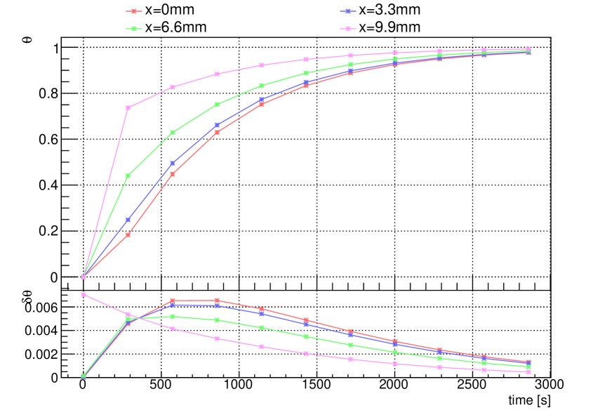
Figure 14: Evolution of the thermal gauge (top pad) and its uncertainty (bottom pad), as a function of the absolute time, for four different values of depth within the sheet.

4 Sensitivity analysis

In this section, we will briefly remind different ways to measure the sensitivity of the output of a model to its inputs. A brief recap of the concept of sensitivity analysis (SA) will be done, before focusing on the use-case and investigating the evolution of the sensitivity indexes through time, for two dimensionless positions: $x_{ds}=0.3$ and $x_{ds}=0.8$.

The use-case application is done following a classical approach: starting with a screening analysis which is quick but not very precise. Once conclusions are drawn from the previous step, a more meticulous investigation can be done using quantitative methods, to get, for instance, the Sobol coefficients of the model under investigation. The starting point will always be the definition of the input variables as gaussian-modelled objects, stored in the TDataServer.

⬇

//Create the TDataServer object

TDataServer *tds = new TDataServer("tds", "The dataserver");

//Create the normally-distributed inputs (given name, mean and standard deviation)

tds->addAttribute( new TNormalDistribution("thickness",e,de));

tds->addAttribute( new TNormalDistribution("conductivity",lambda,dlambda));

tds->addAttribute( new TNormalDistribution("capacity",Crho,dCrho));

tds->addAttribute( new TNormalDistribution("mass",rho,drho));

At the end of this section, a list of the other available methods is given along with their possible improvements in the next few years.

4.1 Introduction to sensitivity analysis

If one can consider that the inputs are independent one to another, it is possible to study how the output variance changes when fixing $X_{i}$ to a certain value $x_{i}^{*}$. This variance denoted by ${\rm Var}(Y|X_{i}=x_{i}^{*})$ is called the conditional variance and depends on the chosen value of $X_{i}$. In order to study this dependence, one should consider ${\rm Var}(Y|X_{i})$, the conditional variance over all possible $x_{i}^{*}$ value, which is a random variable and, as such, it can have an expectation, $E({\rm Var}(Y|X_{i}))$. As the theorem of the total variance states that ${\rm Var}(Y)={\rm Var}(E(Y|X_{i}))+E({\rm Var}(Y|X_{i}))$ under the assumption of having $X_{i}$ and $Y$ two jointly distributed random variables, it becomes clear that the variance of the conditional expectation can be a good estimator of the sensitivity of the output to the specific input $X_{i}$. The more common and practical normalised index in order to define this sensitivity is given by

$$S_{i}=\frac{{\rm Var}(E(Y|X_{i}))}{{\rm Var}(Y)}.$$ (24)

This normalised index is often called the first order sensitivity index and quantifies the impact of the input $X_{i}$ on the output, but does not take into account the amount of variance explained by interactions between inputs. It can actually be made with the crossed impact of this particular input with any other variable or combination of variables, leading to a set of $2^{n_{X}}-1$ indexes to compute. A full estimation of all these coefficients is possible and would lead to a perfect break down of the output variance. It has been proposed by many authors in the literature and is referred to with many names, such as functional decomposition, ANOVA method (ANalysis Of VAriance), HDMR (High-Dimensional Model Representation), Sobol’s decomposition, Hoeffding’s decomposition… A much simpler index, which takes into account the interaction of an input $X_{i}$ with all other inputs, is called the total order sensitivity index or $S_{T_{i}}$ ([31] and can be computed as

$$S_{T_{i}}=1-S_{\bar{i}}=1-\frac{{\rm Var}(E(Y|X_{\bar{i}}))}{{\rm Var}(Y)},$$ (25)

where $\bar{i}$ represents the group of indexes that does not contain the $i$ index. These two indexes (the first order and total order) are referred to as the Sobol coefficients. They satisfy several properties and their values can be interpreted in several ways:

• $\sum S_{i}\leq 1$: should always be true.

• $\sum S_{i}=1=\sum S_{T_{i}}$: the model is purely additive, or in other words, there are no interaction between the inputs and $S_{i}=S_{T_{i}}\;\forall i=1,\ldots,n_{X}$.

• $1-\sum S_{i}$ is an indicator of the presence of interactions.

• $S_{T_{i}}-S_{i}$ is a direct estimate of the interaction of the i-Th input with all the other factors.

4.2 Screening method

4.2.1 Introduction to the Morris method

The Morris method [25] is an effective screening procedure that robustifies the One-factor-At-a-Time protocol (OAT). Instead of varying every input parameter only once (leading then to a minimum of $n_{X}+1$ assessments of the code/function, with an OAT technique), the Morris method repeats this OAT principle $r$ times (practically, it is between 5 and 10 times), each time being called a trajectory or a replica. Every trajectory begins from a randomly chosen starting point (in the input parameters space). In order to do so, it computes Elementary effects (later on called EE), defined as

$$EE^{t}_{i}=EE_{i}(\mathbf{x}^{t})=$$

$$\frac{y(x^{t}_{1},\ldots,x^{t}_{i}+\Delta^{t}_{i},\ldots,x^{t}_{n_{X}})-y(x^{t}_{1},\ldots,x^{t}_{i},\ldots,x^{t}_{n_{X}})}{\Delta^{t}_{i}}$$

where $\Delta^{t}$ is the chosen variation in the trajectory $t$. This variation can be set by the user, but the default (recommended, because it is said to be optimal [32]) value is $\Delta=\frac{p}{2(p-1)}$, where $p$ is the level, that describes in how many interval, the range should be split. The resulting cost (in terms of assessments) is then $r(n_{X}+1)$. This method is schematised in Figure 15 for a problem with three inputs. The hyper-volume is normalised and transformed into an unit hyper-cube. The resulting volume is discretised with the requested level (here, $p=6$) and two trajectories are drawn for different values of the elementary variation.

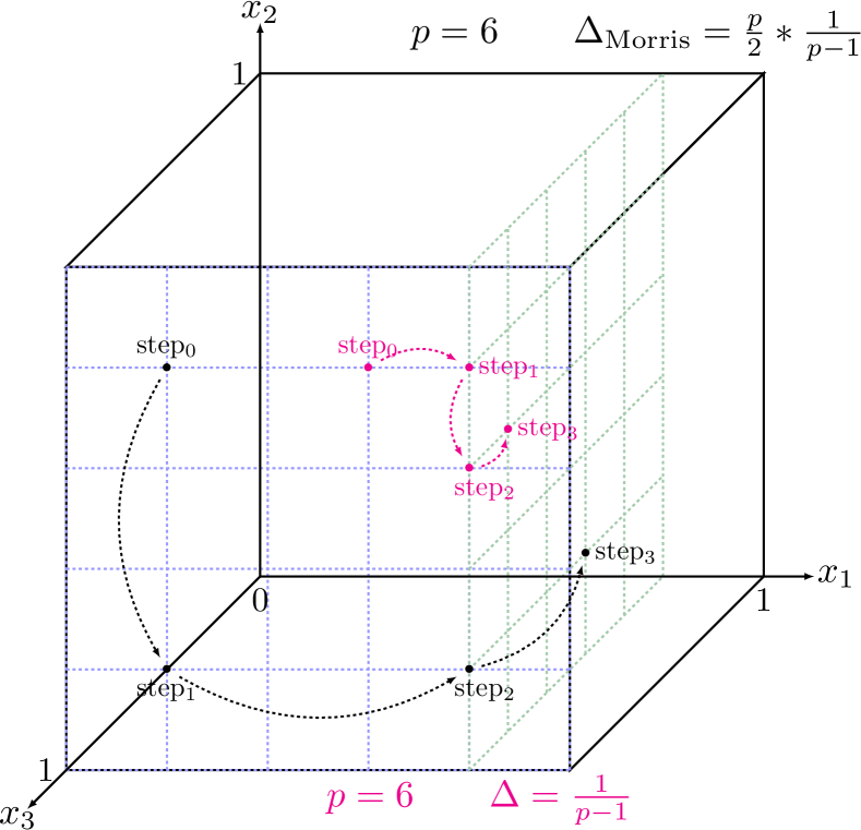
Figure 15: Schematic view of two trajectories drawn randomly in the discretised hyper-volume (with p=6) for two different values of the elementary variation (the optimal one in black and the smallest one in pink).

With the repetition of this procedure $r$ times, it is possible to compute basic statistics on the elementary effects, for every input parameter, as

$$\mu_{i}=\frac{1}{r}\sum^{r}_{t=1}EE^{t}_{i},\;\mu^{*}_{i}=\frac{1}{r}\sum^{r}_{t=1}|EE^{t}_{i}|$$ (26)

and

$$\sigma^{2}_{i}=\frac{1}{r-1}\sum^{r}_{t=1}(EE^{t}_{i}-\mu_{i})^{2}.$$ (27)

The variable $\mu_{i}$ and $\sigma_{i}$ represents respectively the mean and standard deviation of the elementary effects of the i-Th input parameters. In the case where the model is not monotonic some $EE_{i}^{t}$ may cancel each other out, resulting in a low $\mu_{i}$ value even for an important factor. For that reason, a revised version called $\mu_{i}^{*}$ has been created and defined as the mean of the absolute values of the $EE_{i}^{t}$ [33]. The results are usually visualised in the ($\mu^{*}$,$\sigma$) plane.

Even though the numerical results are not easily interpretable, their values can be used to rank the effect of one or several inputs with respect to others, the point being to spot a certain number of inputs that can safely be thrown away, given the underlying uncertainty model assessed.

4.2.2 Implementation in Uranie and application to the use-case

The method has been applied to the thermal exchange model introduced in Section 1.4 which has been slightly changed here for illustration purpose: a new input variable has been added, with the explicit name “useless”. The idea is to shown that it is possible to spot an input whose impact on the output can be considered so small that it can be discarded through the rest of the analysis.

Figures 16a and 16c represent the ($\mu^{*}$,$\sigma$) plane introduced in Section 4.2.1, respectively for $x_{ds}=0.3$ and $x_{ds}=0.8$, measured when the time is set to 572 seconds (about 2 thermal diffusion time). In both cases, it is possible to split the plot in three parts:

• factors that have negligible effect on the output: both $\mu^{*}$ and $\sigma$ are very small. The “useless” input enters this category.

• factors that have linear effects, without interaction with other inputs: $\mu^{*}$ is larger (all variations have an impact) but $\sigma$ is small (the impact is the same independently of the starting point). The massive thermal capacity is a very good illustration of this (as the thermal conductivity or the volumic mass at a smaller scale).

• factors that have non-linear effects and/or interactions with other inputs: both $\mu^{*}$ and $\sigma$ are large. The thickness of the sheet is a perfect illustration of this.

(a) $x_{ds}=0.3$

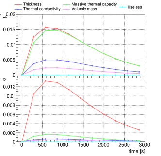
(b) $x_{ds}=0.3$

(c) $x_{ds}=0.8$

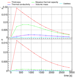
(d) $x_{ds}=0.8$

Figure 16: Measurement of the Morris $\mu^{*}$ and $\sigma$ for $x_{ds}=0.3$ (top) and $x_{ds}=0.8$ (bottom). The a and c parts represent this measurement for a single value of the time, while the b and d parts show the evolution of $\mu^{*}$ (top pad) and $\sigma$ (bottom pad) as a function of the time.

Figures 16b and 16d, on the other hand, show the evolution of both the $\mu^{*}$ and $\sigma$ as a function of the time for the different inputs. Here also, the “useless” inputs can clearly be spotted as negligible through time. Comparing all the other curves, one has to decide the number of other inputs that can be kept into consideration, given the time and memory consumption of a single calculation, but also the physics underlying this behaviour. For the thermal exchange example, considering that the code is fast and the number of inputs is small, the only variable dropped thanks to this method is the “useless” one.

In practice, the main steps used to obtain these results are gathered in the following block:

⬇

//Create the Morris object (given dataserver, the function, the number of trajectories and the variation (level))

TMorris * scmo = new TMorris(tds, "theta", ntrajectories, nlevel);

//Compute the indexes

scmo->computeIndexes();

4.3 The Fast method

4.3.1 Introduction

The Fourier Amplitude Sensitivity Test, known as FAST [34, 35] provides an efficient way to estimate the first order sensitivity indexes. Its main advantage is that the evaluation of sensitivity can be carried out independently for each input factor, using just a dedicated set of runs, because all the terms in a Fourier expansion are mutually orthogonal. To do so, it transforms the $n_{X}$-dimensional integration into a single-dimension one, by using the transformation

$$X_{i}=G_{i}(\sin(\omega_{i}\times s)),$$

where ideally, $\{\omega_{i}\}$ is a set of angular frequencies said to be incommensurate (meaning that no frequency can be obtained by linear combination of the other ones when using integer coefficients) and $G_{i}$ is a transformation function chosen in order to ensure that the variable is sampled accordingly with the probability density function of $X_{i}$. The parametric variable $s$ evolves in $[-\infty,\infty]$ and the vector $(X_{1}(s),\ldots,X_{n_{X}}(s))$ traces out a curve that fills the entire $n_{X}$-dimensional research volume. When both $G_{i}$ and $\omega_{i}$ are properly chosen, one can approximate the following relations:

$$E(Y) =\frac{1}{2\pi}\int_{-\pi}^{\pi}f(s)ds$$ (28)

$${\rm Var}(Y) =\frac{1}{2\pi}\int_{-\pi}^{\pi}f^{2}(s)ds-E^{2}(Y)$$

$$\approx 2\sum_{k=1}^{\infty}(A_{k}^{2}+B_{k}^{2}),$$ (29)

where $f(s)=f(G_{1}(\sin(\omega_{1}s)),\ldots,G_{n_{X}}(\sin(\omega_{n_{X}}s))$ and $A_{k}$ and $B_{k}$ are the Fourier coefficients:

$$A_{k} = \frac{1}{2\pi}\int_{-\pi}^{\pi}f(s)\cos(ks)ds$$ (30)

$$B_{k} = \frac{1}{2\pi}\int_{-\pi}^{\pi}f(s)\sin(ks)ds.$$ (31)

4.3.2 Implementation in Uranie and application to the use-case

This method is applied to the thermal exchange model. The first order coefficient is obtained by estimating the variance for a fundamental $\omega_{i}$ and its harmonics, which can be done by using the second half of Equation (29) running over $p$ instead of $k$ and replacing the index by $p.\omega_{i}$. A cut-off $M$ has to be chosen for the sum and is called the interference factor. Knowing that, the contribution to the output variance of a certain frequency, i.e. the first order sensitivity index, can be expressed from Equations (30) and (31) as

$$S_{i}=\frac{\sum_{p=1}^{M}(A_{p.\omega_{i}}^{2}+B_{p.\omega_{i}}^{2})}{\sum_{i=1}^{n_{X}}\sum_{p_{i}=1}^{M}(A_{p_{i}\omega_{i}}^{2}+B_{p_{i}\omega_{i}}^{2})}$$ (32)

The results are gathered in Figure 17 which shows the evolution of the first order coefficients, as a function of the time, for the four input variables of the model. The histograms are stacked, which means that the contribution of every inputs can be seen as the area represented by the corresponding colour, while the upper limit of the histograms is the sum of all the contributions. Figures 17a and 17b show the evolution as a function of time respectively for $x_{ds}=0.3$ and $x_{ds}=0.8$. The conclusions drawn here are in agreement with the ones from the Morris method in Section 4.2.2:

• the impact of the volumic mass uncertainty is negligible;

• the two most important contributions are coming from the massive thermal capacity and thickness uncertainties;

• the relative importance of the impact of the massive thermal capacity uncertainty with respect to the thickness one seems to increase once we are getting closer to the centre of the sheet.

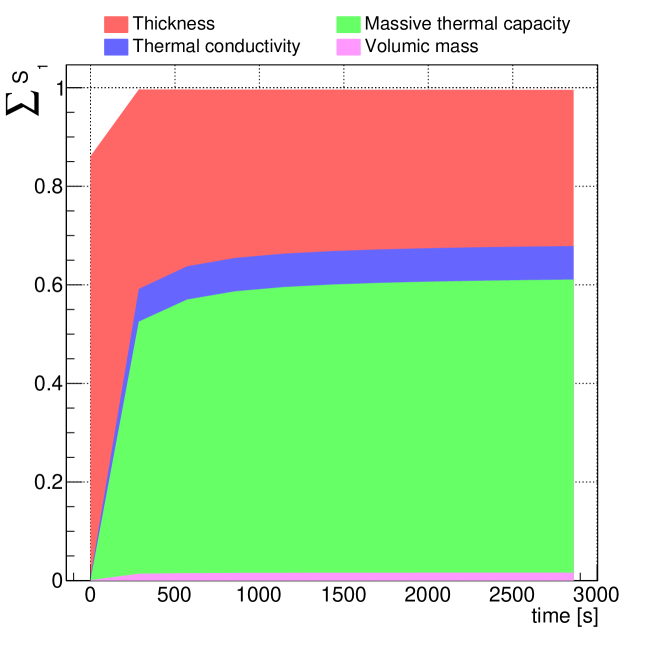
(a) $x_{ds}=0.3$

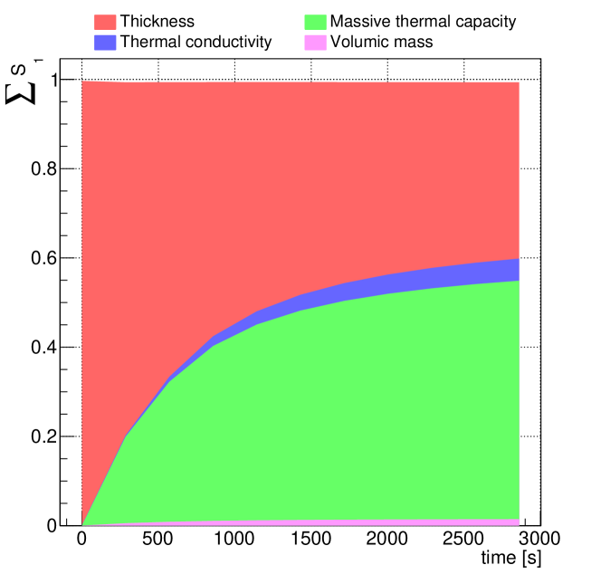
(b) $x_{ds}=0.8$

Figure 17: Measurement of the first order coefficients, with the FAST method, for $x_{ds}=0.3$ (a) and $x_{ds}=0.8$ (b), as a function of time.

On the other hand, by investigating the results in Figure 16, the only possible statement about the impact of the thickness uncertainty was that this factor had either a non-linear effect and/or interaction with other inputs. Here, as the sum of the first order coefficients is equal to 1 for both dimensionless position, it seems reasonable to state that the model has no strong interaction but that the impact of the thickness uncertainty might be a non-linear effect.

In practice, the main steps used to obtain these results are gathered in the following block:

⬇

//Create the Fast object (givan dataserver, the function and the number of locations)

TFast * tfast = new TFast(tds, "theta", ns);

//Choose the interference level

tfast->setM(_M)

//Compute the indexes

tfast->computeIndexes();

4.4 The Sobol method

4.4.1 Introduction

The Sobol method is a Monte-Carlo-based estimation that provides the first and total order sensitivity indexes (respectively introduced in Equations (24) and (25)) at the cost of requiring a total of $n_{S}(n_{X}+2)$ code assessments. Instead of generating a single design-of-experiments, the idea is to produce two of them, called M and N whom size is set to $n_{S}\times n_{X}$ (both matrices are different and independent random samplings). A schematic view of this method, called the pick-and-freeze method, can be found in Figure 18.

The first step is to compute the first order sensitivity index, based on the measurement of the numerator, ${\rm Var}(E(Y|X_{i}))$, which can be written $E(E(Y|X_{i})^{2})-E(E(Y|X_{i}))^{2}$. Since the second part of previous formula is equivalent to the output expectation, the calculation of the first order indexes requires es- timates of $E(E(Y|X_{i})^{2})$, ${\rm Var}(Y)$ and $E(Y)$. The matrix $M$ is passed to the code and $n_{S}$ assessments are done to get a vector of outputs (shown as the first line of Figure 18). The i^th column of $N$ is then replaced by the $M$’s one (pick), creating a new $N_{i}$ matrix which is provided to the code, for an additional cost of $n_{S}\times n_{X}$ assessments. This steps is represented by the second line and the right-part of the third line in Figure 18 and the total cost for the first indexes estimation is $n_{S}(n_{X}+11)$ code assessments.

Finally the total order indexes are computed starting from the right-hand side of Equation (25), which looks very much alike Equation (24) used to compute the first order but instead of a condition on having $i$ known (frozen), it is the exact opposite: the condition is to freeze all the columns but $i$. It is doable as this is the only difference between the $N$ and $N_{i}$ matrices. The total order indexes are thus obtained by passing the $N$ matrix to the code, leading to $n_{S}$ additional code assessments, as shown by the left part of the third line in Figure 18.

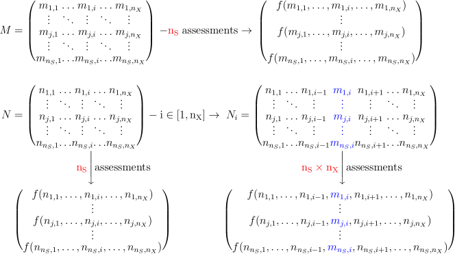
Figure 18: Description of the method used to compute the Sobol coefficients from two matrices.

4.4.2 Implementation in Uranie and application to the use-case

Different implementations of the pick-and-freeze method have been proposed throughout the literature. In Uranie, a single dedicated method gathers the results from several of them ([36, 37]…). One of them in particular is providing the coefficient values along with an estimation of their 95% confidence level ([38]). By re-writing a Sobol coefficient as a correlation coefficient, one can get, under certain hypothesis a confidence level using the Fisher’s transformation rule that applies on empirical correlation coefficients determination.

As for all the methods detailed in this paper, this one has been applied to our thermal exchange model to compute both the first and total order coefficients. The results are gathered in Figure 19 which shows the evolution of both the first and total order coefficients, as a function of time, for the four input variables of the model, along with their 95% confidence interval. In Figures 19a and 19b, the upper part (the first order coefficients) and the lower one (the total order coefficients) are displayed and a reasonable agreement between both order can be found. It leads, once more, to the conclusion that the model has no interaction, as already stated in Section 4.3.2 (for both $x_{ds}=0.3$ and $x_{ds}=0.8$).

(a) $x_{ds}=0.3$

(b) $x_{ds}=0.8$

Figure 19: Evolution of both the first (top pad) and total order (bottom pad) coefficients, as a function of time, with the Sobol method, for $x_{ds}=0.3$ (a) and $x_{ds}=0.8$ (b), along with their 95% confidence interval.

In order to compare these results and the ones presented in Figure 17, the first order coefficients estimated with the Sobol method are represented as stacked histograms in Figure 20. Here again, the contribution of every inputs can be seen as the area represented by the corresponding colour, while the upper limit of the histograms is the sum of all the contributions. Figures 20a and 20b show the evolution as a function of time respectively for $x_{ds}=0.3$ and $x_{ds}=0.8$.

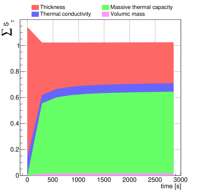
(a) $x_{ds}=0.3$

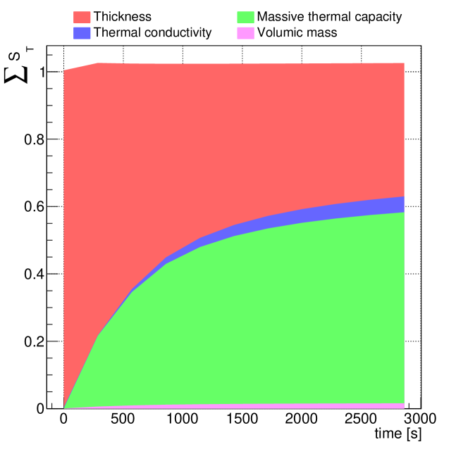
(b) $x_{ds}=0.8$

Figure 20: Measurement of the first order coefficients, with the Sobol method, for $x_{ds}=0.3$ (a) and $x_{ds}=0.8$ (b), as a function of time.

In practice, the main steps used to obtain these results are gathered in the following block:

⬇

//Create the Sobol object (given the dataserver, the function and the number of locations)

TSobol * tsobol = new TSobol(tds, "theta", ns);

//Compute the indexes

tsobol->computeIndexes();

4.4.3 To go further

These methods to estimate either a ranking or more quantitative indicators, such as the Sobol coefficients, have dedicated options to change the way the computations are done. On top of this, there are few other ways to get sensitivity indexes, such as:

• the regression either on values, to get standard regression coefficient (SRC) and partial correlation coefficient (PCC), or on ranks, to get standard regression rank coefficient (SRRC) and partial correlation rank coefficient (PRCC). All indexes can be estimated at once thanks to the algorithm implemented in Uranie [39];

• another Fourier-based algorithm, relying on a different paradigm, called Random Balance Design (RBD) [40];

5 Optimisation

Each optimisation study has its own peculiarities and it often requires to grope one’s way forward, before finding an interesting solution. Most commonly, when dealing with optimisation, there are:

• one or more objectives that one wants to minimise (or maximise).

• decision variables that have a clear influence on the objectives.

• some constraints either on the decision variables, on combination of some of them, or on objectives (defining the search domain)

For every problem, it is compulsory to choose an optimisation algorithm, which is a crucial part of the optimisation procedure. It is possible to divide these algorithms into two different categories:

• local ones: they allow mono-criterion optimisation, with or without constraints. They are generally computationally efficient, but can not be used in parallel and tend to be trapped in local optima.

• global ones: they allow multi-objective optimisation, with or without constraints. They are suitable for problems with many local optima, but are computationally expensive. However, they are easily parallelisable.

Uranie offers several possibilities, either by interfacing external library, as already stated in Section 1.2, or through the use of a dedicated package, called Vizir [41], developed at CEA, whose aim is to offer evolutionary algorithms to solve multi-objective problems.

5.1 Single-objective optimisation problem

5.1.1 Introduction

In the case of a single criterion problem, the optimisation procedure is equivalent to the minimisation of a function $f(\mathbf{x})$ which is called the cost function or the objective function. The optimisation leads to the determination of a minimum (that can be called optimum) that can either be global (there is no $\mathbf{x^{\prime}}$ in the research volume such as $f(\mathbf{x^{\prime}})<f(\mathbf{x_{min}})$) or local (same relation as before, but only in the vicinity of $\mathbf{x_{min}}$). In the case where a maximum should be determined, all the techniques remained, but the objective is changed (inverted) to get back to a minimum search.

In order to do so, Uranie offers many solutions thanks to its external dependencies:

Minuit

It is ROOT’s package to perform single-objective optimisation problem, without constraint. It provides two algorithms

• Simplex: it does not use the first derivatives, it is insensitive to local optima, but without guarantee of convergence.

• Migrad: a fairly sophisticated gradient descent one that is able to escape from some local optima.

NLopt

It is a library for nonlinear optimisation providing algorithms for single-objective optimisation problem, with or without constraint. The list of algorithms implemented in Uranie can be found in [2] along with a small description of their principle, taken from NLopt [9].

5.1.2 Application to the use-case

In this section, a calibration of some of the parameters of our thermal exchange model is performed. Indeed, performing the calibration of a code comes down to finding the optimal set of parameters of the code which minimises the distance between reference values and computations from the code. In Uranie, two distances are currently implemented:

• the root mean square deviation;

• the weighted root mean square deviation.

The starting point is the following: one has done a set of thirty computations or measurements on a PTFE sheet without keeping notes of the experimental conditions. Given that the sheet is made out of PTFE, several intrinsic properties are known, such as the thermal conductivity ($\lambda$), the massive thermal capacity ($C_{\rho}$) and the volumic mass ($\rho$). On the other hand, there are two remaining unknown parameters: the thickness of the sheet ($e$) and the thermal exchange coefficient value ($h$).

The Simplex algorithm (from Minuit optimisation package) is used to minimise the root mean square deviation between the reference thermal gauge values and the ones from every optimisation steps once the parameters under study have been changed. Since this is a local algorithm, the starting point in the ($e$, $h$) plane has to be chosen beforehand (it is represented with a red marker in Figure 21b). A default step value is set for both parameters and the tolerance threshold is chosen, along with a maximum number of calculation, both being the optimisation stopping criteria. The optimisation is run leading to the results presented in Figure 21.

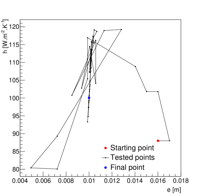
(a) Evolution of the objective

(b) $e$ and $h$ value

Figure 21: Evolution of the cost function as a function of the considered optimisation step (a). Evolution of the parameters from the initial point (red marker) to the optimal found one (blue marker) in the objective ($e$,$h$)-plane (b).

Figure 21a shows the evolution of the objective function with respect to the iteration of the optimisation algorithms. This evolution can be investigated along with the parameter variations shown in Figure 21b: from the chosen starting point in red, every optimisation steps is represented with a black marker and linked to the rest of the already done estimation through a black line. The optimisation has stopped after 52 steps, heading to best estimated value for our parameters of $e_{best}=.01$ and $h_{best}=100.076$ (the blue point in Figure 21b). These values are in agreement with the reference ones which have produced the original set of points (these values are shown in Table 1).

5.1.3 Possible limitations

This solution is very efficient, mainly because the code to be run is quick. In the case of a very time-memory and/or cpu consuming code, this might have been difficult: as the Simplex algorithm is sequential, no parallelism is possible. There are more refined techniques to perform optimisation with less code assessments (using surrogate model for instance), as introduced in the following sections.

5.2 Multi-objectives optimisation

5.2.1 Introduction

The optimisation problem, in the multi-objective case, can then be expressed as the minimisation of the function $F(\mathbf{x})=(f_{1}(\mathbf{x});\,f_{2}(\mathbf{x});\,\ldots;\,f_{n}(\mathbf{x}))$ where $n$ is the number of objectives imposed and $F$ is the complete cost function. In some cases, the objectives can be combined, for instance by doing a weighted (or not) sum, resulting in a new objective over which the optimisation is performed. This is what is done in the example above where the difference between the thirty output values in the reference set and the newly computed ones, for a given set of parameters, are combined into a single objective. Unlike this case, the multi-objective hypothesis is that no overall optimum can be determined when it is not be possible to quantify a relation between the objectives. In this case, when two solutions $x_{1}$ and $x_{2}$ are possible, $x_{1}$ dominates $x_{2}$ if it does as good as the latter for all the objectives and strictly better for at least one. The optimisation goal is then to get a group of solutions that are said to be not dominated: no solution out of this group dominates them, and in the group either. There is no best point, unless an external constraint or preference is imposed, usually with hindsight.

The group of not-dominated solutions is called the Pareto set and its representation in the objective space is called the Pareto front. Figure 22a shows an academic example of a pure analytic model with two objectives depending only on one variable. In this simple case, the Pareto set is shown in pink, as the area in between both criterion’s minimum. Now looking in the objective space in Figure 22b, all the solutions are shown in black and the corresponding Pareto front is, once more, depicted in pink.

(a) variable space

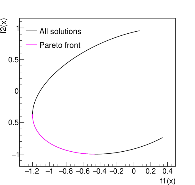
(b) objective space

Figure 22: Naive example of an imaginary optimisation case relying on two objectives that only depend on a single input variable.

5.2.2 The Vizir package

In Uranie multi-objectives optimisation issues are dealt with the Vizir package, which gathers several solutions, all developed at CEA, regarding the considered evolutionary algorithms and the way to make them evolve (genetic or swarm algorithm, single or island evolution…). In any case, the aim is to get a certain number $N$ of solutions to describe correctly both the Pareto set and front, and the analysis can be described in few key steps (shown in Figure 23) and detailed below.

1. Initialisation. Create randomly, only using the research space definition, a population of the requested size ($N$). The first evaluation is performed for all candidates, meaning that the criteria and constrains will be tested and the results will be stored in a vector for all candidates. This step is represented as a black box in Figure 23, followed by the evaluation shown as the orange box.

2. Ranking. The rank affected to a candidate under study corresponds to the number of other candidates that dominate it. The best candidates have then a rank 0 (they are not-dominated), following by those with rank 1, rank 2…

3. Convergence test. This test (green box in Figure 23) can reach three possible states:

   • all the tested candidates are not-dominated. The algorithm has converged and the loop is stopped;

   • not all candidates are not-dominated but the maximum number of evaluation has been reached. The algorithm has stopped without having converged. The optimisation should be restarted (maybe changing the configuration);

   • not all candidates are not-dominated and the maximum number of evaluation is not reached.

4. Re-generation. In the latter case of the convergence test, a fraction of the lowest-ranked candidates ($\lambda$) is kept (purple box in Figure 23) and used to produce a new generation, the crossing procedure depending on the chosen algorithm (blue box in Figure 23). This resulting population, made out of the selected ($\lambda N$) and re-generated candidates ($1-\lambda N$), is re-evaluated.

Figure 23: Schematic description of the needed steps of an optimisation procedure, when this one is performed with Vizir.

These steps are more thoroughly explained in [2]. Even though this library can be used on its own for multi-objective optimisation, the example provided below will embedded it in the context of efficient global optimisation (EGO).

5.3 Efficient global optimisation

This section layouts another optimisation possibility to look for a minimum using a global technique. The efficient global optimisation, known as EGO [42], is first introduced and then applied to a simple mono-dimensional example that will fully illustrate the principle. Finally the calibration problem discussed in Section 5.1.2 will be investigated with this technique, to help appreciate the pros and cons of this method.

5.3.1 Introduction

The EGO technique is the perfect illustration of method combination, introduced in Section 1.3, where all the building blocks are already implemented in Uranie. It might be useful in the case where the code is high time/cpu/memory consuming (so one wants to limit as much as possible the computation) given that there might be several local minimum in which one doesn’t want to fall (preventing from using local optimisation such as gradient ones for instance). Instead of having to choose a starting point (as done in Section 5.1.2), the idea is to provide a training database which is supposed to be representative of the problem, so whose size cannot be too small with respect to the dimension of the ongoing analysis. Once done, a kriging model is constructed.

Let $f_{min}=min(y_{1},\ldots,y_{n_{t}})$ be the current best function value ($n_{t}$ being the size of the kriging training database). It is true, that before computing the output of the code for a given input vector $\mathbf{x}$, we are uncertain about the value $y(\mathbf{x})$. On the other hand, $y(\mathbf{x})$ is not completely unknown as we can assimilate it to $\hat{y}(\mathbf{x})$ its realisation through the kriging surrogate model, which is provided along with its standard deviation $s(\mathbf{x})$. With this hypothesis, it is possible to compute the probability of the real value to be below the actual minimum $f_{min}$. Different distances below the line $y=f_{min}$ , are associated with different density values. If we weight all these possible improvements by the associated density value, we get what we call the “expected improvement” (EI). The improvement for a given point $\mathbf{x}$ is $I=max(f_{min}-\hat{y}(\mathbf{x}),0)$ which is a random variable as $\hat{y}(\mathbf{x})$ models our uncertainty about the code’s value at $\mathbf{x}$. To get the expected improvement, from here, we simply take the expected value of this random variable:

$$E[I(\mathbf{x})] = E[max(f_{min}-\hat{y}(\mathbf{x}),0)]$$

$$= (f_{min}-\hat{y}(\mathbf{x}))\Phi\left(\frac{f_{min}-\hat{y}(\mathbf{x})}{s(\mathbf{x})}\right)$$

$$+ s(\mathbf{x})\phi\left(\frac{f_{min}-\hat{y}(\mathbf{x})}{s(\mathbf{x})}\right)$$ (33)

In this equation, $\phi(.)$ and $\Phi(.)$ are respectively the standard normal density and its cumulative distribution. These two contributions are bringing a trade-off between exploring within a promising area and exploring where the uncertainty of the surrogate model is large. The latter contribution bringq back the global aspect requested.

Once done, the next step consists in searching the maximum of the expected improvement which is a positive definite function. This is done by using the genetic algorithm, as this search is actually an optimisation: the aim is to minimise the the opposite EI criteria, providing the best candidate. The code is then run on this specific location, which is then included in the training database. The kriging model is re-build, using the updated training database and a new location is determined, following the exact same recipe.

5.3.2 Application to the thermal exchange model

The idea here is to apply the EGO method on a mono-dimensional problem to get plots that would perfectly illustrate the way this procedure works. This will be done by working on a simple function which is an extension of our thermal exchange model. In Section 1.4.2 one of the first hypothesis to get an analytic solution was to fix the thermal exchange coefficient $h$ to a constant value. This is known to be a rough approximation and a more rigorous way to describe the evolution of this coefficient through time is actually given by the following equation:

$$h(t)=\frac{h_{max}-h_{min}}{1+\beta(t-t_{max})^{2}},\;\beta=\frac{h_{max}-h_{0}}{t_{max}^{2}(h_{0}-h_{min})}$$ (34)

whose behaviour is represented in Figure 24.

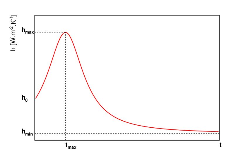
Figure 24: Modelisation of the evolution of the thermal exchange coefficient as a function of the time.

This equation depends on 4 parameters: the initial and asymptotic value of the thermal exchange coefficient (which can be measured respectively at the very beginning and after a very long time on a given experiment). The other parameters are the coordinate of the maximum, whose measurement can be turned into an optimisation by looking for the minimum of the opposite function $-h(t)$. This is exactly what has been done and this analysis can be summarised in Figure 25 where, in the upper part of every pad, the blue line is the real ”unknown” function used, the black points are the training database, the red line is the approximation given by the kriging model along with its uncertainty and the green point is the latest point included in the training database from the previous iteration. The bottom pad of every plot shows the inverted expected improvement ($-EI$) which is minimised using the evolutionary algorithm to determine the next location to be included in the training database.

(a) 0 new points

(b) 1 new points

(c) 2 new points

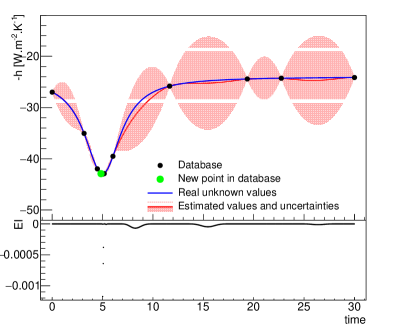
(d) 4 new points

(e) 5 new points

(f) 9 new points

Figure 25: Evolution of the kriging surrogate model in red, compared to the real (supposed unknown) function in blue, as a function of the time for different number of locations in the training database. These ones are represented as black dots, expect for the latest-introduced one, spotted in green. The bottom part of every plot represents the evolution of the expected improvement.

Going though Figure 25, one can find back the different steps described in Section 5.3.1

Figure 25a

Starting point, the training database is made out of 4 locations, and the uncertainty on the model at several places are large. One of the location is close to the real minimum and is the current $f_{min}$. From the EI, the next location to be computed will be on the other side of the real minimum (where the estimated values from the kriging model are small and the uncertainties are large).

Figure 25b

One more location has been computed and added to the training database (it is the current new $f_{min}$). The updated kriging model has changed tremendously and the lowest boundary is the next location to be computed. This is the perfect illustration of the global aspect of this method: a gradient would have been down to check for a smaller minimum, disregarding the fact that other part of the phase space might be really mis-modelled..

Figure 25c

One more location has been computed and added to the training database upon which the kriging model has been updated. The next location to be computed (from the EI curve) is very close to the real minimum.

Figure 25d

Two more locations have been added to the training database (among which a new $f_{min}$ in agreement with the real minimum). As the model uncertainty band for the locations around $f_{min}$ is small, the next location to be computed is the highest boundary, which, once more, shows the global behaviour of this protocol.

Figure 25e

Once the highest boundary has been included, few more locations around the real minimum will be tested.

Figure 25f

The method will start computing the closest location to $f_{min}$ with the largest uncertainty.

The steps described in Figure 25 converge quickly toward an estimation of the parameters $t^{*}_{max}=5$ and $h^{*}_{max}=42.9999$ which are in very good agreement with the injected values ($t^{Real}_{max}=5$, $h^{Real}_{max}=43$). The only sensitive aspect is to be able to stop the method: one can not use a tolerance criteria as it could prevent the exploration needed to conserve the global behaviour. The only remaining option is to set a maximum number of location to be added, or to put a threshold on the Leave-One-Out $Q^{2}$ criterion of the kriging model. This criterion is not really focusing on the minimum description, but more on agreement of the kriging model.

For illustration purpose only, the same method has been applied to the calibration problem introduced in Section 5.1.2. The idea is to compare the results given in Figure 21 to the one presented in Figure 26. A training database of 20 locations has been generated and the algorithm has been run over 32 more computations in order to get the same number of code assessments (1560, as already computed in Section 5.1.3).

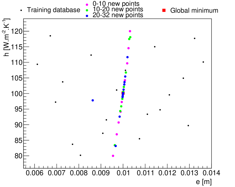
Figure 26: Training database (black points) and the 32 new points computed using the EGO algorithm (purple, green and blue points) for the calibration problem discussed in Section 5.1.2. The best minimum found is represented as the red box.

Figure 26 shows the training database (black points) and the 32 new locations computed using the EGO algorithm (blue points) along with the best minimum found (red box). The newly computed locations are split into three categories: the first ten ones in purple, the following ten ones in green and the last twelve ones in blue. Thanks to this splitting, it is possible to check that the optimisation exploration remains global as there can be green and even blue new locations computed far away from the global minimum. However, most of the locations included by the EGO method are along a clear line, showing the shape of the minimum valley in the ($e$,$h$)-plane (that was also visible in Figure 21b). Here is the different level of agreement obtained on the parameters, as a function of the number of locations computed (so the number of assessments):

8 new locations:

the accuracy obtained on $e$ and $h$ is respectively $\sim 0.3$% and $\sim 1.5$%

21 new locations:

the accuracy obtained on $e$ and $h$ is respectively $\sim 0.01$% and $\sim 0.3$%

28 new locations:

the accuracy obtained on $e$ and $h$ is respectively $\sim 0.01$% and $\sim 0.2$%

6 Perspectives

In this section, an important property, not discussed up to now but common to many Uranie’s methods is briefly discussed, along with the perspective of development considered by the team.

6.1 Parallelism

The fact that the code under consideration might be very consuming in terms of time, cpu and/or memory has been raised several times throughout this paper. This, along with the fact that some of method might need also a great deal of internal computations, even without the external code, show the clear necessity to have parallelism strategy to benefit from the recent hardware paradigm: the number of cpu is no-more a limiting criteria while on the other hand, cpu frequency has reached a plateau and memory access tend to become problematic ([43]).

In order to deal with this, the Uranie team is working on two different aspects:

code assessments distribution:

this is the way an external code is called. Several strategies are implemented in Uranie:

• forking the code on a local node or on a list of resources listed as available at the initialisation. This is duplicating the code and the Launcher module (see Figure 1) will distribute the computations.

• shared-memory distribution. This technique is using the pthread protocol to distribute the code assessments through the Relauncher module (see Figure 1). This, as all memory-shared strategy, can suffer from race conditions (which might only depend on whether the code used is thread-safe).

• split-memory distribution. This technique relies on an mpirun distribution of the computation through the Relauncher module (see Figure 1). This has the advantage of not suffering from race conditions, but the variables used can only be numerical-based (Uranie can also handle string variables as input/output of an external code).

internal calculation distribution:

Mainly available for the k nearest neighbour and artificial neural networks, the idea is to used the very high number of graphics processing unit (GPU) given in a reasonable graphical card, to perform internal computation (in the already-introduced case, the training of the synaptic weight for instance). This is done using CUDA, provided by the NVIDIA company ([11]).

The proper use of these solutions allows to benefit from the structure of the new computers and the grid upon which the Uranie platform can be installed.

6.2 Perspective

The Uranie platform is in perpetual evolution to keep in touch with the latest improvement of both the academic and the industrial world, bearing in mind the possible needs of its community as well. There are many possible fields of interests toward which the developing team is investigating, among which:

• the usage of Markov Chain. Starting from the Bayesian inference needs, to be able to get the ”a posteriori” parameters distributions, the idea would be to handle a Gibbs ([44]) or Metropolis-Hastings ([45]) implementation to move to our own Hamiltonian Markov chain ([19]) component to overcome possible slowness and convergence problems (particularly in high dimensions).

• the development of ”deep learning” capacities. The first step toward this is to change the actual perceptron to allow to use several outputs and to get more than one hidden layer of neurons. Other developments are considered, such as the use of recurrent neural network (RNN, [46]) or deep belief network (DBN, [47]).

• the development of many-criteria optimisation algorithms. With more than 3 criteria to optimise, the optimisation is said to be many-criteria, and there are several possibilities under study such as the knee point driven evolutionary algorithm ([48]) or algorithm based on decomposition on a grid, as the Many Objective Evolutionary Algorithm based on Dominance and Decomposition (MOEADD [49]). The aim is also to be able to have constraints on these criteria.

These leads are not exhaustive and the priority with which they might be considered can depend as well from the needs and requests from our community.

References

- [1] R. Brun, F. Rademakers, ROOT: An object oriented data analysis framework, Nucl. Instrum. Meth. A389 (1997) 81–86. doi:10.1016/S0168-9002(97)00048-X.
- [2] J.-B. Blanchard, Methodological reference guide for uranie v3.11.0, Tech. rep., CEA, DEN/DANS/DM2S/STMF/LGLS/RT/17-006/A (2017).
- [3] J.-B. Blanchard, User manual for uranie v3.12.0, Tech. rep., CEA, DEN/DANS/DM2S/STMF/LGLS/NT/2017-62273/A, to be released (2017).
-
[4]
D. Van Heesch, Doxygen: Source code
documentation generator tool (2008).
URL http://www.doxygen.org - [5] K. Martin, B. Hoffman, An open source approach to developing software in a small organization, Ieee Software 24 (1).
- [6] M. Feathers, B. Lepilleur, Cppunit cookbook (2002).
-
[7]
J. C. Meza, R. A. Oliva, P. D. Hough, P. J. Williams,
Opt++: An object-oriented
toolkit for nonlinear optimization, ACM Transactions on Mathematical
Software 33 (2).
doi:10.1145/1236463.1236467.
URL http://doi.acm.org/10.1145/1236463.1236467 - [8] M. Frigo, S. G. Johnson, The design and implementation of FFTW3, Proceedings of the IEEE 93 (2) (2005) 216–231, special issue on “Program Generation, Optimization, and Platform Adaptation”.
- [9] S. G. Johnson, The nlopt nonlinear-optimization package, http://ab-initio.mit.edu/nlopt (2008).
- [10] E. Gabriel, G. E. Fagg, G. Bosilca, T. Angskun, J. J. Dongarra, J. M. Squyres, V. Sahay, P. Kambadur, B. Barrett, A. Lumsdaine, R. H. Castain, D. J. Daniel, R. L. Graham, T. S. Woodall, Open MPI: Goals, concept, and design of a next generation MPI implementation, in: Proceedings, 11th European PVM/MPI Users’ Group Meeting, Budapest, Hungary, 2004, pp. 97–104.
- [11] C. Nvidia, Nvidia cuda c programming guide, Nvidia Corporation 120 (18) (2011) 8.
- [12] E. de Rocquigny, N. Devictor, S. Tarantola, Uncertainty in industrial practice: a guide to quantitative uncertainty management, John Wiley & Sons, 2008.
-
[13]
N. Wiener, The homogeneous chaos,
American Journal of Mathematics 60 (4) (1938) 897–936.
URL http://www.jstor.org/stable/2371268 -
[14]
R. H. Cameron, W. T. Martin, The
orthogonal development of non-linear functionals in series of fourier-hermite
functionals, Annals of Mathematics 48 (2) (1947) 385–392.
URL http://www.jstor.org/stable/1969178 - [15] R. G. Ghanem, P. D. Spanos, Stochastic Finite Elements: A Spectral Approach, Springer-Verlag New York, Inc., New York, NY, USA, 1991.
-
[16]
M. Baudin, J.-M. Martinez,
Polynômes de chaos sous
Scilab via la librairie NISP, in: 42èmes Journées de Statistique,
Marseille, France, France, 2010.
URL https://hal.inria.fr/inria-00494680 -
[17]
W. McCulloch, W. Pitts, A logical
calculus of the ideas immanent in nervous activity, The bulletin of
mathematical biophysics 5 (4) (1943) 115–133.
doi:10.1007/BF02478259.
URL http://dx.doi.org/10.1007/BF02478259 -
[18]
F. Rosenblatt, Principles
of neurodynamics: perceptrons and the theory of brain mechanisms, Report
(Cornell Aeronautical Laboratory), Spartan Books, 1962.
URL https://books.google.fr/books?id=7FhRAAAAMAAJ - [19] R. M. Neal, et al., Mcmc using hamiltonian dynamics, Handbook of Markov Chain Monte Carlo 2 (11).
- [20] G. Matheron, La théorie des variables régionalisées, et ses applications, Fasicule 5 in Les Cahiers du Centre de Morphologie Mathématique de Fontainebleau.
- [21] J.-M. Martinez, A. Marrel, N. Gilardi, F. Bachoc, Krigeage par processus gaussiens. Librairie gpLib, Tech. rep., CEA DEN/DANS/DM2S/STMF/LGLS/RT/12-026/A (2012).
-
[22]
F. Bachoc, Estimation paramétrique
de la fonction de covariance dans le modèle de krigeage par processus
gaussiens : application à la quantification des incertitues en simulation
numérique, Ph.D. thesis, Mathématiques appliquées, Paris 7, thèse de
doctorat dirigée par Garnier, Josselin (2013).
URL http://www.theses.fr/2013PA077111 - [23] J.-M. Martinez, Tutorial du krigeage dans uranie, Tech. rep., CEA DEN/DANS/DM2S/STMF/LGLS/NT/13-014/A (2015).
-
[24]
M. D. McKay, R. J. Beckman, W. J. Conover,
A comparison of three methods for
selecting values of input variables in the analysis of output from a computer
code, Technometrics 42 (1) (2000) 55–61.
doi:10.2307/1271432.
URL http://dx.doi.org/10.2307/1271432 - [25] D. Morris, J. Mitchell, Exploratory designs for computational experiments, Journal of Statistical Planning and Inference 43 (1995) 381–402.
- [26] L. Pronzato, W. Muller, Design of computer experiments: space filling and beyond, Statistics and Computing 22 (3) (2012) 681–701.
- [27] R. L. Iman, W. J. Conover, A distribution-free approach to inducing rank correlation among input variables, Communications in Statistics - Simulation and Computation 11 (3) (1982) 311–334. doi:10.1080/03610918208812265.
-
[28]
J. H. Halton, Algorithm 247:
Radical-inverse quasi-random point sequence, Commun. ACM 7 (12) (1964)
701–702.
doi:10.1145/355588.365104.
URL http://doi.acm.org/10.1145/355588.365104 -
[29]
I. Sobol’,
On
the distribution of points in a cube and the approximate evaluation of
integrals, USSR Computational Mathematics and Mathematical Physics 7 (4)
(1967) 86 – 112.
doi:http://dx.doi.org/10.1016/0041-5553(67)90144-9.
URL http://www.sciencedirect.com/science/article/pii/0041555367901449 -
[30]
K. Petras, Fast calculation of
coefficients in the smolyak algorithm, Numerical Algorithms 26 (2) (2001)
93–109.
doi:10.1023/A:1016676624575.
URL http://dx.doi.org/10.1023/A:1016676624575 - [31] T. Homma, A. Saltelli, Importance measures in global sensitivity analysis of nonlinear models, Reliability Engineering and System Safety 52 (1996) 1–17.
- [32] A. Saltelli, S. Tarantola, F. Campolongo, M. Ratto, Sensitivity Analysis in Practice: A Guide to Assessing Scientific Models, Wiley, New York, 2004.
- [33] A. Saltelli, S. Tarantola, F. Campolongo, M. Ratto, T. Andres, J. Cariboni, D. Gatelli, M. Saisana, Global Sensitivity Analysis: The Primer, Wiley, New York, 2008.
-
[34]
G. McRae, J. Tilden, J. Seinfeld,
Global
sensitivity analysis: a computational implementation of the fourier amplitude
sensitivity test (fast), Computers & Chemical Engineering 6 (1) (1982) 15
– 25.
doi:http://dx.doi.org/10.1016/0098-1354(82)80003-3.
URL http://www.sciencedirect.com/science/article/pii/0098135482800033 -
[35]
A. Saltelli, R. Bolado,
An
alternative way to compute fourier amplitude sensitivity test (fast),
Computational Statistics & Data Analysis 26 (4) (1998) 445 – 460.
doi:http://dx.doi.org/10.1016/S0167-9473(97)00043-1.
URL http://www.sciencedirect.com/science/article/pii/S0167947397000431 - [36] A. Saltelli, Making best use of model evaluations to compute sensitivity indices, Computer Physics Communications 145 (2002) 280–297.
- [37] H. Monod, C. Naud, D. Makowski, Uncertainty and sensitivity analysis for crop models, In D. Wallach, D. Makowski, and J. W. Jones, editors, 2006.
- [38] J.-M. Martinez, Analyse de sensibilité globale par décomposition de la variance, Tech. rep., GdR Ondes et Mascot Num, institut Henri Poincaré (2011).
- [39] R. Iman, M. Shortencarier, J. Johnson, FORTRAN 77 program and users guide for the calculation of partial correlation and standardized regression coefficients, Sandia National Laboratories, 1985.
-
[40]
S. Tarantola, D. Gatelli, T. Mara,
Random
balance designs for the estimation of first order global sensitivity
indices, Reliability Engineering & System Safety 91 (6) (2006) 717 – 727.
doi:https://doi.org/10.1016/j.ress.2005.06.003.
URL http://www.sciencedirect.com/science/article/pii/S0951832005001444 - [41] G. Arnaud, Manuel d’utilisation de Vizir distribué v2.0, Tech. rep., CEA, SFME/LGLS/RT/10-001/A (2010).
- [42] D. R. Jones, M. Schonlau, W. J. Welch, Efficient global optimization of expensive black-box functions, Journal of Global optimization 13 (4) (1998) 455–492.
- [43] U. Drepper, What every programmer should know about memory, Red Hat, Inc 11 (2007) 2007.
- [44] G. Casella, E. I. George, Explaining the gibbs sampler, The American Statistician 46 (3) (1992) 167–174.
- [45] S. Chib, E. Greenberg, Understanding the metropolis-hastings algorithm, The american statistician 49 (4) (1995) 327–335.
- [46] T. Robinson, F. Fallside, A recurrent error propagation network speech recognition system, Computer Speech & Language 5 (3) (1991) 259–274.
- [47] G. E. Hinton, To recognize shapes, first learn to generate images, Progress in brain research 165 (2007) 535–547.
- [48] X. Zhang, Y. Tian, Y. Jin, A knee point-driven evolutionary algorithm for many-objective optimization, IEEE Transactions on Evolutionary Computation 19 (6) (2015) 761–776.
- [49] K. Li, K. Deb, Q. Zhang, S. Kwong, An evolutionary many-objective optimization algorithm based on dominance and decomposition, IEEE Transactions on Evolutionary Computation 19 (5) (2015) 694–716.