Stability and Dynamic Control of Underlay Mobile Edge Networks

Abstract

This paper studies the stability and dynamic control of underlay mobile edge networks. First, the stability region for a multiuser edge network is obtained under the assumption of full channel state information. This result provides a benchmark figure for comparing performance of the proposed algorithms. Second, a centralized joint flow control and scheduling algorithm is proposed to stabilize the queues of edge devices while respecting the average and instantaneous interference power constraints at the core access point. This algorithm is proven to converge to a utility point arbitrarily close to the maximum achievable utility within the stability region. Finally, more practical implementation issues such as distributed scheduling are examined by designing efficient scheduling algorithms taking advantage of communication diversity. The proposed distributed solutions utilize mini-slots for contention resolution and achieve a certain fraction of the utility optimal point. The performance lower bounds for distributed algorithms are determined analytically. The detailed simulation study is performed to pinpoint the cost of distributed control for mobile edge networks with respect to centralized control.

I Introduction

I-A Background and Motivation

The predictions of Cisco visual networking index indicate that mobile data traffic has grown $4,000$-fold over the past ten years [1]. One main driver for such an unprecented growth is the surge of computationally powerful devices close to the network edge like smartphones, tablets, connected vehicles, smart meters, femtocells, wireless-enabled industrial robots/drones [2, 3, 4], to name a few. Consequently, there is an increasing tendency to perform communication and signal processing tasks at the network edge in next generation LTE-A networks through the enablement of technologies such as fog computing, WiFi direct, D2D/IoT communication, cognitive radio and femto-cells [2, 5, 6]. This paradigm shift in networking automatically triggers the need for a thorough investigation of multi-tier network architectures in which multiple network tiers with different underlying technology components can co-exist together in the same spectrum.

The most prominent advantage of mobile edge networking is to ease the communication and computation burden on the core network by making use of the immersive distributed network of devices at the network edge. As such, data generated at the edge stays at the edge for communication and computation purposes such as stream mining and embedded artificial intelligence, without a need to traverse the core network anymore. This approach not only improves the efficiency of spectrum usage, but also has a great potential for enhancing the network performance expressed in terms of capacity, coverage, energy efficiency and end-to-end delay [7, 8].

The main challenge now is to adapt new approaches for networking at large so that direct communication among edge devices can seamlessly coexist with inbound and outbound data traffic from the core network in the same frequency band. As is common in the cognitive radio literature [9], two outstanding approaches for the coexistence of different technologies at the network edge and core can be conceived to be inband/outband underlay and overlay communications. The main focus of this paper will be on the inband underlay communications in which edge devices utilize the same spectrum with the core access point (AP) in a two-tier network architecture. In this setup, the radio frequency spectrum is the shared communication resource whose access must be regulated for network stability and performance optimization. This will be done at the network edge by designing smart interference management strategies and appropriate cross-layer resource allocation algorithms.

Important use cases of mobile edge networking include high data rate wireless services, IoT applications and industrial control systems [2]. Many data-intensive services at the network edge such as virtual reality, online gaming, video sharing, vehicle-to-vehicle communication and proximity-aware social networks require small end-to-end delay of incoming data packets. The same also holds correct for many IoT applications and industrial control systems with strict deadlines on sensor-plant communication and control actions. Therefore, in addition to queue stability, an overall utility for communicating over the network edge must be maximized, as a measure of service satisfaction in different applications. To this end, we combine a variety of basic networking mechanisms such as flow control and scheduling in the context of underlay mobile edge networking. In particular, by modeling the entire problem as that of a network utility maximization, we develop the utility-optimal cross-layer dynamic flow control and scheduling mechanisms achieving the optimum utility point within the stability region subject to various interference power constraints at the core network. The main analytical tool used for this purpose is the stochastic network optimization framework put forward in [10]. The motivation to follow this approach is to investigate network stability and optimality jointly as is also done in [11, 12] to address fairness issues by investigating the scheduling problem and network utility maximization (NUM) together.

I-B Contributions

The main contributions of this paper are two-fold. First, a thorough analysis for interference-aware mobile edge networking is provided. In doing so, we derive the stability region for edge devices operating under interference constraints at the network core. The notion of stability region here refers to the set of rates achievable by any feasible flow control and scheduling policies not violating predefined hard interference limitations at the core AP. The interference regulated stability region is compared with the one without any QoS guarantees at the core network, which leads to the quantification of rate loss due to interference-aware operation of the edge network.

We then formulate a resource allocation problem for interference-aware edge networking as a NUM problem, in which the optimal scheduling of edge devices is implemented at the MAC layer, while the flow control is realized at the transport layer. We propose a cross-layer dynamic control algorithm for solving the scheduling and flow control problem jointly. It is shown that the proposed cross-layer design achieves a utility point arbitrarily close to the maximum achievable utility. In particular, the flow control algorithm moves the rate vector to the Pareto boundary of the stability region, while the scheduling algorithm ensures that the core network constraint qualifications are met.

As a second contribution, we examine the problem of practical implementation of the above cross-layer design in the absence of a centralized scheduler. Specifically, we design simple but efficient distributed channel access algorithms, called channel-aware distributed schedulers, where the edge devices decide to transmit or not based on their local information (i.e., their channels and queue backlogs). The proposed algorithms are channel-aware in the sense that they are able to take channel variations into account for scheduling decisions.

We obtain analytical performance bounds on the dynamic control of the edge network based on the proposed channel-aware distributed schedulers. Now, the utility optimal point achieved through a centralized scheduler can no longer be guaranteed due to availability of limited information in the distributed mode of operation. To quantify the performance loss, we show that we can achieve an $\alpha^{*}$-fraction of the utility optimal point and obtain an analytical characterization of the parameter $\alpha^{*}\in\left[0,1\right]$. $\alpha^{*}$ can be adjusted as a function of the contention level and the number of mini-slots used by the distributed scheduler to resolve contention. We demonstrate the advantages of the proposed distributed solutions by means of an extensive simulation study.

II Related Work

Our results in this study crosscut a wide range of literature including mobile edge networking, D2D/IoT communication, cognitive radio networks and multi-tier HetNets. Hence, we will only mention the papers that are most relevant to ours, mostly focusing on the literature in underlay D2D communication and cognitive radio networks.

The papers such as [13, 14, 15, 16, 17, 18, 19] investigate the resource allocation problem for underlay D2D/IoT networks. In [13, 14], the authors consider a single cell scenario with a cellular base-station (BS) and two D2D users sharing the same spectrum. Power control is exercised on the BS and the spectrum usage of the D2D pairs is optimized by considering sum rate as the objective function subject to energy/power constraints under non-orthogonal and orthogonal sharing mode. In order to further improve the gain from intra-cell spectrum reuse, properly pairing cellular and D2D users for sharing the same resources was studied in [15, 16].

In particular, [15] considers the control of interference from D2D links to the cellular users by limiting the maximum transmit power of the D2D users. In [16], the authors employ the knowledge of spatial interference for D2D receivers to maximize network capacity with multiuser MIMO. Cellular users in the vicinity of the interference-limited area are not scheduled. The optimal power allocation problems for D2D networks are analyzed in [17, 18, 19]. The authors in [17] and [18] show that the problem of optimal power allocation and mode selection are not tractable. They propose an alternative greedy heuristic algorithm to lessen interference at the core cellular AP. The proposed scheme is practical but cannot prevent excessive signaling overhead. The authors in [19] propose a method to identify power efficiency for D2D communication, which is a function of transmission rate and power consumption of the devices.

The papers [20, 21, 22] focus on performance optimization of D2D networks subject to certain QoS constraints. The authors in [20] consider throughput-optimal resource allocation problem with minimum rate guarantees for both D2D and regular users. The paper [21] formulates the problem of maximizing the system throughput with minimum data rate requirements by means of the particle swarm optimization framework to obtain a solution. In [22], they formulate fair resource allocation for D2D networks as an integer programming problem, which is NP-hard. Hence, they propose a sub-optimal solution that captures the interplay between different elements of the optimization problem in different phases. D2D caching networks are investigated in [23] and [24]. The authors in [23] analyze the scalability of multi-hop wireless communications for the case of replicated content across the nodes. The system model in [24] incorporates traditional microwave and millimeter-wave D2D links, and they show that in non-asymptotic regimes, the proposed D2D system model offers very significant throughput gains with respect to BS-only schemes.

The above papers indicate the potential of D2D networks to improve spectrum efficiency and data throughput at the network edge if the interference can be regulated at the core cellular networks. The main point of difference between the current work and those above is the cross-layer design approach developed in this paper to address queue stability, scheduling and flow control jointly. Different from them, we obtain a parametric characterization for the stability region of devices at the network edge under hard interference limitations at the network core. Further, we obtain a cross-layer scheduling and flow control algorithm maximizing the overall network utility within this stability region without violating interference limitations.

In addition to above work, our results in this paper are also related to those on resource allocation and opportunistic scheduling for underlay cognitive radio networks (CRNs) [25, 26, 27, 28, 29, 30, 31, 32, 33, 34]. The authors in [25] investigated the optimal power control and the resulting throughput scaling laws for underlay CRNs under average interference power constraints at the primary users. The same results are extended to the fully distributed case and partial cooperation case between secondary and primary networks in [26] and [27], respectively. The papers such as [28] and [29] analyze the performance of underlay CRNs subject to instantaneous interference power constraints to optimize outage probability and some queuing performance metrics.

Opportunistic scheduling for CRNs is studied in [30], where Lyapunov optimization tools are used to design flow control, scheduling and resource allocation algorithms. Explicit performance bounds are derived. In [31], the authors analyzed stable throughput for a primary multi-access system, where a secondary user (SU) receives packets from two primary users (PU) and relays them using the superposition coding technique when the primary slot is idle. The paper [32] studies the tradeoff between packet delay and energy consumption in a cooperative cognitive network. One common cooperation method is cooperative relaying [33]. In cooperative relaying, the SU receives the failed PU packets and relays them to the primary destination on the next transmission opportunity. An additional relay queue is needed at the SU source for this purpose. Ashour et al. in [34] proposed an admission control algorithm as well as randomized service at the relay queue and analyzed stable throughput in CRNs. One distinctive aspect of the current paper from the existing work in underlay CRNs above is a thorough analysis of the distributed implementation of scheduling and flow control algorithms in a mobile edge networking setting. An efficient distributed scheduler is designed explicitly, and the loss from such a distributed mode of operation is characterized analytically.

III System Model, Scheduling Policy and Edge Network Stability

In this section, we will introduce the details of our system model and the definitions of the main concepts that are used throughout the paper in relation to this model.

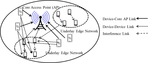
Figure 1: Network model consisting of $N$ edge device pairs that share a common frequency band with a core access point.

III-A System Model

Our primary aim is to propose an efficient cross-layer design for mobile edge networks that lead to optimum utility point stabilizing the queues at edge devices. Both centralized and distributed approaches are investigated, with the centralized cross-layer algorithm (i.e., joint flow control and scheduling) being the benchmark to evaluate the performance of distributed algorithms. To this end, we consider a group of edge devices forming $N$ distinct links and sharing the same frequency band with a core network AP, as shown in Fig. 1. Note that these communication links can be considered to be among D2D pairs, cognitive devices or femtocell users at the network edge depending on the application scenario. The edge devices are in close proximity of each other so that they can reach to their intended receivers in a single hop, yet they cause excessive interference to each other when multiple pairs are active at the same time. This leads to a fully connected interference graph topology with collision model for the edge network.

The devices operate in slotted time with slot indices represented by $t\in\mathbb{N}$. The link qualities vary over time according to the block fading model, in which the channel gain is constant over a time slot and changes from one slot to another independently according to a common fading distribution. We use $h_{i}(t)$, $i=1,\ldots,N$, to represent the direct channel gain between the transmitter and receiver of the $i$th link. These direct channel gains are independent and identically distributed (iid) over users as well as over time. Operating in the same frequency band, the devices also cause interference to the core AP in Fig. 1. We denote the interference channel gain between the transmitter of the $i$th edge link and the core AP by $g_{i}(t)$ for $i=1,\ldots,N$. Furthermore, there may be other surrounding edge devices and core devices transmitting data to the core AP, not too close but causing some non-negligible interference to the edge network in question. We denote the total interference caused to the pair $i$ by $I_{i}(t)$ for $i=1,\ldots,N$. Again, interference channel gains obey to the iid block fading model (possibly with a different distribution than that of the direct channel gains) as described above. We assume that the channel gains and inter-edge network interference levels are drawn from continuous distributions. For notational simplicity, we often use the vector notation $\boldsymbol{h}(t)=\left[h_{1}(t),\ldots,h_{N}(t)\right]$, $\boldsymbol{g}(t)=\left[g_{1}(t),\ldots,g_{N}(t)\right]$ and $\boldsymbol{I}(t)=\left[I_{1}(t),\ldots,I_{N}(t)\right]$ to denote the channel gains and interference values more compactly.

For the sake of comprehending the interplay between the scheduling decisions at the MAC layer and the flow control decisions at the transport layer better, it is assumed that no power control is exercised at the physical layer of the network edge and all devices transmit at a constant power level $P$ over all time slots. This assumption will help us to distill the effect of physical layer parameters on the interactions of the upper layer scheduling and flow control protocols, which is the main focus of the current paper. In this setting, an important quantity of interest that determines the network performance is the rates (measured in units of bits/slot) offered over a communication link during time slot $t$. We assume that these communication rates are described by the functions $R_{i}(t)$ (as functions of transmission power levels, channel gains and interference levels) for $i=1,\ldots,N$. Even though we do not assume any specific functional form for $R_{i}(t)$, which is usually determined by the coding and communication technologies embedded in the transceiver circuits of the edge devices, we require that $R_{i}(t)$ has a bounded second moment, i.e., ${\mathsf{E}}\left[{R_{i}(t)^{2}}\right]\leq R_{max}^{2}$ for all $t\in\mathbb{N}$. The significance of the rate function $R_{i}(t)$ in our analysis is that it will determine the service rates of the network layer queues maintained at the network edge.

An application runs at the application layer of each edge device, and generates the bits to be stored at the transport layer queues. These bits are accepted to the network layer according to a flow control mechanism that runs at the transport layer. We let $A_{i}(t)$ represent the amount of data (in bits per slot) that enters the network layer at the beginning of time slot $t$ and is stored at a network layer queue with size $Q_{i}(t)$ at edge device $i$, $i\in\left\{1,\ldots,N\right\}$. The relationship between these important network parameters at the queue level is displayed in Fig. 2.

It is assumed that the input rate $A_{i}(t)$ is admissible in the sense that $A_{i}(t)\leq A_{max}$ for all $t\in\mathbb{N}$, and it has a long-term average $x_{i}$, i.e., $x_{i}=\limsup_{T\rightarrow\infty}\frac{1}{T}\sum_{t=1}^{T}A_{i}(t)$. The utility obtained by the communication over the $i$th link, $U_{i}\left(x_{i}\right)$, is a function of the long-term average rate $x_{i}$. We assume that $U_{i}(0)=0$, and $U_{i}\left(x\right)$ is a continuously differentiable, monotonically increasing and concave function of its argument. This concludes the description of our system model.

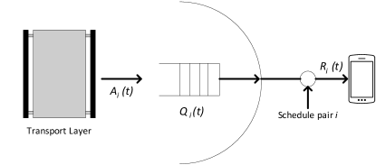
Figure 2: Queue model for edge pair $i$.

III-B Scheduling Policy

Due to close geographical proximity of edge devices in our model, only one device pair in the edge network can communicate its data reliably over its respective wireless communication link. Hence, a scheduling decision must be made at the beginning of each time slot to select an appropriate user based on the current (both direct and interference) channel conditions. For this purpose, roughly speaking, a scheduling policy should determine which set of links to be activated in each time slot for data transmission.

Definition 1

A scheduling policy $\boldsymbol{\cal I}:\mathbb{R}_{+}^{3N}\mapsto[0,1]^{N}$ is a vector-valued function $\boldsymbol{{\cal I}}\left(\boldsymbol{h}(t),\boldsymbol{g}(t),\boldsymbol{I}(t)\right)=\left[{\cal I}_{1}\left(\boldsymbol{h}(t),\boldsymbol{g}(t),\boldsymbol{I}(t)\right),\ldots,{\cal I}_{N}(\boldsymbol{h}(t),\boldsymbol{g}(t),\boldsymbol{I}(t))\right]^{\intercal}$ that maps the direct and interference channel states to scheduling probabilities, i.e., ${\cal I}_{i}\left(\boldsymbol{h}(t),\boldsymbol{g}(t),\boldsymbol{I}(t)\right)\in[0,1]^{N}$ for each $i\in\left\{1,\ldots,N\right\}$, and satisfies the feasibility constraint $\sum_{i=1}^{N}{\cal I}_{i}\left(\boldsymbol{h}(t),\boldsymbol{g}(t),\boldsymbol{I}(t)\right)\leq 1$.

For ease of notation, we refer to ${\cal I}_{i}\left(\boldsymbol{h}(t),\boldsymbol{g}(t),\boldsymbol{I}(t)\right)$ as ${\cal I}_{i}(t)$ in the rest of the paper. It should be noted that scheduling policies given in Definition 1 constitute a collection of randomized control mechanisms for the edge network in question specifying scheduling probabilities for each pair of device. Implicit in this definition, a scheduling policy does not allow two links to be active simultaneously due to the topological constraints of our network model. More explicitly, once scheduling probabilities are identified for all links in the edge network for time slot $t\in\mathbb{N}$, only one of them is selected for transmission by using the probability distribution induced by $\boldsymbol{{\cal I}}(t)$ over the set of edge device indices to determine the index of the selected link.

An important subset of the randomized scheduling policies is the deterministic ones. We say that a scheduling policy $\boldsymbol{{\cal I}}(t)=\left[{\cal I}_{1}(t),\ldots,{\cal I}_{N}(t)\right]^{\intercal}$ is a deterministic scheduling policy if ${\cal I}_{i}(t)$ is either zero or one for all $i\in\left\{1,\ldots,N\right\}$ and for all time slots $t\in\mathbb{N}$. It will be shown below that the use of randomized scheduling policies will facilitate the mathematical analysis of the collection of optimization problems leading to the network stability region by turning them into convex optimization problems, whilst the solutions of these optimization problems lie in the set of deterministic scheduling policies.

III-C Edge Network Stability

In this part, we will provide the details of the notion of the edge network stability by relating the scheduling policies to the queue level dynamics of edge devices. To this end, we will first put forward the notion of interference-aware edge network operation. All the network stability definitions presented afterwards will be with respect to this notion of interference-aware operation.

The main communication paradigm of interest that we focus on for the coexistence of an edge network with core network users in the same spectrum is the underlay paradigm [9]. The main idea underpinning the underlay communication paradigm is that the edge network can utilize the same spectrum with the core AP as long as it does not cause harmful degradation to the data communication at the core AP by keeping the interference levels (instantaneous and average) below pre-specified interference threshold values. This leads to the interference-aware edge network operation, formally defined as below.

Definition 2

An edge network is said to be an interference-aware network if the average and instantaneous interference power levels that it causes to the core network AP is bounded above by the pre-specified interference threshold values as

$$\sum_{i=1}^{N}{\mathsf{E}}\left[{Pg_{i}(t){\cal I}_{i}(t)}\right]\leq\gamma\mbox{ and }{\cal I}_{i}(t)=0\mbox{ if }Pg_{i}(t)>\nu,$$ (1)

where $\gamma$ and $\nu$ denote the upper limits on the aggregate average and individual instantaneous interference powers from all links in the edge network, respectively.

This definition makes the coupling between the scheduling policies and the restrictions due to the interference-aware operation explicit. In particular, the optimum scheduling policy achieving the maximum communication rates that can be stably supported by an interference-aware edge network must strike a balance between choosing the best link at the network edge and respecting the radio etiquette rules arbitrating the spectrum access rights between edge devices and the core AP. The above interference constraints are primarily designed to safeguard two types of data traffic at the core network against the harmful edge network interference. The average interference constraint in (1) is for delay-insensitive data traffic (e.g., text messaging) for which the messages are encoded and decoded over many time slots. On the other hand, the instantaneous interference constraint in (1) is for delay-sensitive data traffic (e.g., video streaming) for which the messages are encoded and decoded over a single time slot. An edge network may not know the type of data traffic at the core AP at any given particular time, and hence must respect both constraints simultaneously.

Next, we formally define the concept of the stability of an interference-aware edge network. As is standard [10], stability here refers to being long-term averages of expected queue sizes finite, i.e., $\limsup_{T\rightarrow\infty}\frac{1}{T}\sum_{t=0}^{T-1}{\mathsf{E}}\left[{Q_{i}(t)}\right]<\infty$. Further, we say that the edge network is stable under $\boldsymbol{{\cal I}}(t)$ if the network layer queues of all edge devices are stable. An important concept that expands upon the definition of network stability and relates the flow control and scheduling mechanisms for an edge network is the network stability region, which is defined as below.

Definition 3

The network stability region of an interference-aware edge network, denoted by $\Lambda$, consists of all arrival rate vectors $\boldsymbol{x}=\left(x_{1},x_{2},\ldots,x_{N}\right)^{\intercal}$ such that there exists a scheduling policy $\boldsymbol{{\cal I}}(t)$ satisfying the conditions below for all $i\in\left\{1,\ldots,N\right\}$ and $t\in\mathbb{N}$:

$${\mathsf{E}}\left[{{\cal I}_{i}(t)R_{i}(t)}\right]\geq x_{i},$$ (2)

$$\sum_{i=1}^{N}{\mathsf{E}}\left[{Pg_{i}(t){\cal I}_{i}(t)}\right]\leq\gamma,$$ (3)

$${\cal I}_{i}(t)=0\mbox{ if }Pg_{i}(t)>\nu,\mbox{and }\sum_{i=1}^{N}{\cal I}_{i}(t)\leq 1.$$ (4)

The constraints in (3) and (4) are due to the interference-aware operation of the edge network and the feasibility condition. The constraint in (2) is the classical necessity constraint for the queue stability describing the fact that the incoming rate to the network layer queues should be equal to or smaller than the outgoing service rate, which depends on the choice of the scheduling policy in our particular edge networking scenario [35].

In the next section, we will obtain the Pareto boundary of the network stability region, where no feasible and interference-aware scheduling policy can stabilize the edge network when the arrival rates are beyond this boundary. This will provide a complete characterization of $\Lambda$. This characterization will be carried out under the full channel-state information (CSI) assumption. Although helpful in understanding the maximum rates that can be stably supported by an edge network, such a characterization of the network stability region does not provide us with any insights regarding how to design dynamic control mechanisms achieving the rates in $\Lambda$.

To resolve this drawback, we design a dynamic but centralized flow control and scheduling algorithm that achieves all the rates within the network stability region in Section V. The scheduling part of the proposed algorithm provides design insights into how to construct a feasible and interference-aware scheduling mechanism for an edge network. In addition to stabilizing an interference-aware edge network, the proposed algorithm also maximizes the collective utility of the edge devices. The flow control part of the proposed algorithm provides design insights into how to construct flow control mechanism to maximize collective network performance. The distributed solutions achieving these desirable properties up to some performance gaps are given in Section VI.

IV Stability Region for Interference-Aware Edge Networks

In this section, we derive the boundary of the stability region of an interference-aware edge network such that any arrival rate vector outside the closure of the boundary is unattainable. Then, we analyze the effect of interference-aware communication on the network stability region by comparing the boundaries obtained with and without interference constraints.

We begin our analysis by computing the boundary of network stability region. This is equivalent to maximizing the average outgoing (service) rate achieved by edge device $i$ for given average rate values of other devices. Recall that the average arrival rate should be smaller or equal to the average service rate in a stable network. Hence, we say that an arrival rate $x_{i}$ of an edge device $i\in\left\{1,\ldots,N\right\}$ that is larger than this maximized service rate cannot be achieved. Before giving the mathematical description of the problem, the following remark is important. Since we assume that the channels are ergodic and stationary, we utilize the statistical averages in constructing the optimization problem. Hence, we ignore the time index for the sake of notational simplicity in this section. But in the next section, when we perform dynamic control, we again introduce time index back. Further, for notational convenience, let $\Psi$ be the set of all scheduling policies. Therefore, the aim is to maximize ${\mathsf{E}}\left[{{\cal I}_{i}(\boldsymbol{h},\boldsymbol{g},\boldsymbol{I})R_{i}}\right]$, associated with the point ${\mathsf{E}}\left[{{\cal I}_{j}(\boldsymbol{h},\boldsymbol{g},\boldsymbol{I})R_{j}}\right]=\alpha_{j},\forall j\neq i$, by solving the following optimization problem:

$$\max_{\boldsymbol{{\cal I}}\in\Psi} \ {\mathsf{E}}\left[{{\cal I}_{i}(\boldsymbol{h},\boldsymbol{g},\boldsymbol{I})R_{i}}\right]$$ (5)

subject to $$\ {\mathsf{E}}\left[{{\cal I}_{j}(\boldsymbol{h},\boldsymbol{g},\boldsymbol{I})R_{j}}\right]\geq\alpha_{j},\ \forall j\neq i$$ (6)

$${\mathsf{E}}\left[{\sum_{j=1}^{N}P{\cal I}_{j}(\boldsymbol{h},\boldsymbol{g},\boldsymbol{I})g_{j}}\right]\leq\gamma$$ (7)

$${\cal I}_{j}(\boldsymbol{h},\boldsymbol{g},\boldsymbol{I})=0\mbox{ if }Pg_{j}>\nu\mbox{ and }\sum_{j=1}^{N}{\cal I}_{j}(\boldsymbol{h},\boldsymbol{g},\boldsymbol{I})\leq 1,$$ (8)

where the expectations are over the joint distribution of the instantaneous channel gains of direct and interference channels as well as the interference values. We solve the above optimization problem using the dual method that is particularly appealing to our problem structure, whose solution is given in the next theorem.

Theorem 1

A solution of the optimization problem given in (5)-(8) is equal to

$${\cal I}_{j}^{*}(\boldsymbol{h},\boldsymbol{g},\boldsymbol{I})=\begin{cases}1,&\text{ if }W_{j}=\max_{k\in C}W_{k}\\ 0,&\text{otherwise}\end{cases}$$

where $C=\left\{j:W_{j}\geq 0,Pg_{j}\leq\nu\right\}$, $W_{j}=\lambda_{j}^{*}R_{j}-\mu^{*}Pg_{j}$ for all $j\neq i$, $W_{i}=R_{i}-\mu^{*}Pg_{i}$, and $\lambda_{j}^{*}$ and $\mu^{*}$ are Lagrange multipliers associated with the rate and interference constraints in (6) and (7), respectively.

Proof:

Please see Appendix A. ∎

Theorem 1 gives us the optimal scheduling policy $\boldsymbol{{\cal I}}^{*}$ achieving ${\mathsf{E}}\left[{{\cal I}_{j}^{*}(\boldsymbol{h},\boldsymbol{g},\boldsymbol{I})R_{j}}\right]=\alpha_{j}$ for all $j\neq i$. Then, the boundary of the stability region can be attained by varying $\alpha_{j},\forall j\neq i$, and obtaining the points where the average rates of edge device $i$ are maximized. Another important point is that even though we state the optimization problem for the randomized scheduling policies, i.e., ${\cal I}_{j}(\boldsymbol{h},\boldsymbol{g},\boldsymbol{I})\in[0,1]$, the optimal solution turns out to be a deterministic scheduling policy, i.e., ${\cal I}_{j}(\boldsymbol{h},\boldsymbol{g},\boldsymbol{I})$ is either zero or one. In addition, observe that if the condition $Pg_{j}>\nu$ or $W_{j}<0$ for all edge devices, then the channel remains idle. The reason is that the channel conditions are not good enough to access the channel at the expense of the interference caused to the core AP.

As indicated above, there may be time instants during which the channel remains idle in an interference-aware edge network to safeguard the core AP. This will result in a decrease in optimal rates due to under-utilization of the channel. Consequently, it leads to a contraction of the network stability region. To understand this phenomenon better, we also derive the optimum scheduling policy without interference constraints, and compare the achievable rate regions in both cases with and without interference constraints. Following similar arguments above, we have the following optimum scheduling problem

$$\max_{\boldsymbol{{\cal I}}\in\Psi} {\mathsf{E}}\left[{{\cal I}_{i}(\boldsymbol{h},\boldsymbol{g},\boldsymbol{I})R_{i}}\right]$$ (9)

subject to $${\mathsf{E}}\left[{{\cal I}_{j}(\boldsymbol{h},\boldsymbol{g},\boldsymbol{I})R_{j}}\right]\geq\alpha_{j},\ \forall j\neq i$$ (10)

$$\sum_{j=1}^{N}{\cal I}_{j}\left(\boldsymbol{h},\boldsymbol{g},\boldsymbol{I}\right)\leq 1$$ (11)

without interference constraints, whose solution is given by the next theorem.

Theorem 2

A solution of the optimum scheduling problem in (9)-(11) is equal to

$${\cal I}_{j}^{*}(\boldsymbol{h},\boldsymbol{g},\boldsymbol{I})=\begin{cases}1,&\text{ if }\lambda_{j}^{*}R_{j}>\lambda_{k}^{*}R_{k},\ \forall k\neq j\\ 0,&\text{otherwise}\end{cases}$$

where $\lambda_{j}^{*}$ is the Lagrange multiplier associated with the rate constraint in (10).

Proof:

The proof follows the similar lines with the proof of Theorem 1, and hence is skipped to avoid repetitions. ∎

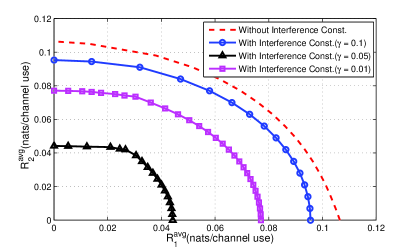
(a) Network stability region for varying interference parameter $\gamma$

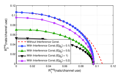
(b) Network stability region for varying interference channel gains.

Figure 3: Network stability region for the communication scenario with two pairs of edge devices, where $R_{i}^{\rm avg}={\mathsf{E}}\left[{{\cal I}_{i}^{*}\left(\boldsymbol{h},\boldsymbol{g},\boldsymbol{I})\right)R_{i}}\right]$.

In Figs. 3a-3b, the stability region for a two-link edge network is illustrated for Rayleigh fading direct and interference channels, in which the communication rate is selected as Shannon capacity, i.e., $R_{i}(t)=\log\left(1+\frac{Ph_{i}(t)}{N_{0}+I_{i}}\right)$. Only average interference power constraint is considered for having clean exposition. We select 10 interfering links to the edge devices, and the mean channel gains of these links are randomly chosen between $0.05$ and $0.2$ to simulate $\boldsymbol{I}$. To plot the stability regions, we varied the rate achieved by the second pair, calculated $\lambda^{*}$ and obtained the boundary rate pair for each point. Recall that $h_{i}$ and $g_{i}$ are the direct and interference channel gains of the $i$th pair, respectively. In Fig. 3a, we take ${\mathsf{E}}\left[{h_{1}}\right]={\mathsf{E}}\left[{h_{2}}\right]=0.4$ and ${\mathsf{E}}\left[{g_{1}}\right]={\mathsf{E}}\left[{g_{2}}\right]=0.2$ to obtain different boundary rate pair for varying interference parameter $\gamma$. As seen in Fig. 3a, when we decrease $\gamma$, i.e., the interference constraint is more stringent, the network stability region shrinks since both pairs have less transmission opportunities to meet the interference constraint. In Fig. 3b, we fixed the value of $\gamma$ at $0.1$ and vary ${\mathsf{E}}\left[{g_{2}}\right]$. As seen in Fig. 3b, when ${\mathsf{E}}\left[{g_{2}}\right]=0.1$, the network stability regions (with and without interference constraints) coincide for small rate values of edge user $1$, where the second pair takes a higher portion of transmissions. This observation results from the fact the interference constraint is inactive in this case and the second pair with smaller interference channel gain transmits predominantly. On the other hand, as ${\mathsf{E}}\left[{g_{2}}\right]$ increases, i.e., ${\mathsf{E}}\left[{g_{2}}\right]=0.2,0.5$ and $1$, the interference experienced by the core AP starts to increase and the network stability region shrinks.

V Control of Underlay Edge Networks with Centralized Scheduling

In the previous section, we characterize the stability region by obtaining maximum rates that an interference-aware edge network can support. In this section, we will present a dynamic control algorithm that will solve a NUM problem while stabilizing the network layer queues in an edge network. To do so, we follow a cross-layer design approach. In the lower layer, the scheduling policy ensures network stability and satisfies the interference requirements. In the upper layer, on the other hand, flow control policy strives to move the network layer arrival rates to the optimal point within the stability region. Since the derived cross-layer algorithm will be a dynamic online algorithm, we will use the time index $t\in\mathbb{N}$ in this section again to indicate its operation in time.

The dynamic cross-layer algorithm takes the queue lengths (both virtual and real queues) and instantaneous direct and interference channel gains as input, and determines the scheduled device $i\in\left\{1,\ldots,N\right\}$ at each time slot as an output. We start our analysis by first formulating the NUM problem and providing the queue dynamics to set the stage for the cross-layer design approach.

V-A NUM Problem Formulation

Our objective is to stabilize the edge network while maximizing the sum of device utilities. That is, we aim to find a solution for the following NUM problem:

$$\max_{\boldsymbol{x}}\ \sum_{i=1}^{N}U_{i}(x_{i})$$ (12)

subject to $$\boldsymbol{x}\in\Lambda.$$ (13)

The objective function in (12) accounts for the total expected utility of edge devices over random stationary channel conditions, interference values and scheduling decisions. The constraint in (13) ensures that network layer arrival rates of edge devices are within the rate region that can be stably supported by the edge network. The above problem could be in principle solved by means of standard convex optimization techniques if the stability region is known in advance. Although this approach may give us an idea about how to select transmission rates, it will not say anything about how we can reach the optimum operating point by relating the solution to the design of edge networks. Thus, in the following subsections, we develop a practical dynamic control algorithm to facilitate our understanding of the interplay between interference requirements and the critical functionalities of edge networks, such as scheduling and flow control.

V-B Queue Dynamics

We assume that there is an infinite backlog of data at the transport layer of each edge device. Our proposed dynamic flow control algorithm determines the amount of traffic injected into the queues at the network layer. The dynamics of the network layer queue of the $i$th edge pair is given as

$$Q_{i}(t+1)=\left[Q_{i}(t)-{\cal I}_{i}(t)R_{i}(t)\right]^{+}+A_{i}(t).$$ (14)

To meet the average interference constraint given in (1), we also maintain a virtual queue

$$Z(t+1) =\left[Z(t)-\gamma+\sum_{i=1}^{N}{\cal I}_{i}(t)Pg_{i}(t)\right]^{+}.$$ (15)

The state of the virtual queue at any given time instant is an indicator on the amount by which we exceed the allowable interference constraint. Thus, the larger the state of these queues, the more conservative our dynamic algorithm has to get towards meeting constraints, i.e., the less transmissions will take place by edge device pairs. The strong stability of virtual queues guarantees that the interference constraints are satisfied in the long run (i.e., see Theorem 5.1 in [10]).

V-C Dynamic Control

The proposed cross-layer dynamic control algorithm is based on the stochastic network optimization framework [10]. This approach enables us to obtain a solution for long-term stochastic optimization problems without requiring an explicit characterization of the stability region. Furthermore, it facilitates the simultaneous treatment of stability and performance optimization by the introduction of virtual queues to transform performance constraints into queue stability problems.

To this end, consider the queue backlog vectors for communication pairs, which are denoted as ${\boldsymbol{Q}}(t)=(Q_{1}(t),\ldots,Q_{N}(t))$ and $Z(t)$. Let $L({\boldsymbol{Q}}(t),Z(t))$ be a quadratic Lyapunov function of real and virtual queue backlogs defined as:

$$L({\boldsymbol{Q}}(t),Z(t))=\frac{1}{2}\left((Z(t))^{2}+\sum_{i=1}^{N}(Q_{i}(t))^{2}\right).$$ (16)

Also, consider the one-step expected Lyapunov drift, $\Delta(t)$, for the Lyapunov function as

$$\Delta(t)={\mathsf{E}}\left[{L({\boldsymbol{Q}}(t+1),Z(t+1))-L({\boldsymbol{Q}}(t),Z(t))|{\boldsymbol{Q}}(t),Z(t)}\right].$$

The aim of the stochastic network optimization framework is to minimize the drift to ensure network stability, which can be achieved by having negative Lyapunov drift whenever the sum of queue backlogs is sufficiently large. Intuitively, this property ensures network stability because whenever the queue backlog vector leaves the stability region, the negative drift eventually drives it back to this region. Furthermore, the following utility-mixed Lyapunov drift

$$\Delta^{U}(t)=\Delta(t)-V{\mathsf{E}}\left[{\sum_{i=1}^{N}U_{i}(A_{i}(t))\ \Big{|}\ {\boldsymbol{Q}}(t),Z(t)}\right]$$ (17)

enables us to maximize the edge network performance in conjunction with the network stability, where the conditional expectation is taken with respect to all common randomness and $V>0$ is a design parameter.

Next, we present the control algorithm that minimizes (17) and provide its optimality in Theorem 3.

Control Algorithm: Making an analogy to back pressure algorithm, we propose the following cross-layer algorithm that executes the following steps at each time $t\in\mathbb{N}$:

1. Upper Layer - Flow control: The flow controller at each edge device observes its current queue backlog $Q_{i}(t)$. It then injects $A_{i}(t)$ bits, where $A_{i}(t)$ is the solution of the following optimization problem:

   $$A_{i}(t)=\operatorname*{argmax}_{0\leq x\leq A_{max}}\{VU_{i}(x)-Q_{i}(t)x\}.$$ (18)

   The design parameter $V>0$ will determine the final performance of the proposed algorithm. The above identity involves maximizing a concave function, which can be easily solved by using convex optimization techniques [36].

2. Lower Layer - Scheduling: A scheduler observes the backlogs in all edge devices and all fading/interference states. Then, it determines the scheduling decision for time slot $t\in\mathbb{N}$, $\boldsymbol{{\cal I}}(t)$, as the following index policy:

   $${\cal I}_{i}(t)=\left\{\begin{IEEEeqnarraybox}[]{[}][c]{l^{\prime}s}1,&if$i =\operatorname*{argmax}_{j \in C} W_j(t)$\\ 0,&otherwise\end{IEEEeqnarraybox}\right.$$

   for all $i\in\left\{1,\ldots,N\right\}$, where $C=\left\{j:W_{j}\geq 0,Pg_{j}(t)\leq\nu\right\}$ and $W_{i}(t)$ is the weight of edge pair $i$ that is given as:

   $$W_{i}(t)=Q_{i}(t)R_{i}(t)-PZ(t)g_{i}(t).$$ (20)

   Specifically, among the edge pairs that satisfy the instantaneous interference constraint, the one having the maximum weight is allowed to transmit at a given time slot. If the set $C$ is an empty set, then no edge pair is scheduled for transmission. If the set $\operatorname*{argmax}_{j\in C}W_{j}(t)$ is not singleton, then any one of edge pairs in this set can be scheduled for transmission. For continuous interference channel states, $\operatorname*{argmax}_{j\in C}W_{j}(t)$ is always singleton if there exists at least one element in $C$.

We note that the parameter $V>0$ in the flow control algorithm determines the extent to which the utility optimization problem is emphasized. Indeed, if $V$ is large relative to the current backlog in the source queues, then the admitted rates $A_{i}(t)$ will be large, increasing the time average utility while consequently increasing the congestion level at the network edge. This effect is mitigated by more conservative flow control decisions as the backlog grows at the source queues. Note that the flow control algorithm is decentralized because the control values for each device require only knowledge of the queue backlogs at edge device pair $i\in\left\{1,\ldots,N\right\}$.

In the scheduling policy, the weight equation (20) consists of a reward term $Q_{i}(t)R_{i}(t)$ and a cost term $PZ(t)g_{i}(t)$. Specifically, the larger the data queue backlog size $Q_{i}(t)$ and/or higher the instantaneous channel rate $R_{i}(t)$, the more likely the transmission from edge pair $i$ occurs. On the other hand, the larger the interference queue backlog size $Z(t)$ (representing the interference level caused to the core AP) and/or higher the interference channel gain $g_{i}(t)$, the less likely the transmission of edge pair $i$ takes place. In this setting, the flow control algorithm strives to maximize collective network utility, whereas the scheduling policy makes sure that the utility maximizing operating point is within the stability region. Indeed, by utilizing the proposed scheduling algorithm, we can achieve any point in the stability region.

Theorem 3

Suppose $\boldsymbol{x^{*}}=[x_{1}^{*},\ldots,x_{N}^{*}]$ is the average arrival rates produced by the proposed dynamic control algorithm. Then, for any flow parameter $V>0$, the dynamic control algorithm yields the following performance bound for the aggregate network utility:

$$\sum_{i=1}^{N}U_{i}(x_{i}^{*}) \geq U^{*}-\frac{B_{1}}{V}$$

while bounding the total long-term expected queue lengths as:

$$\limsup_{T\rightarrow\infty}\frac{1}{T}\sum_{\tau=0}^{T-1}\sum_{i=1}^{N}{\mathsf{E}}\left[{Q_{i}(\tau)}\right] \leq\frac{B_{1}+V\kappa}{\epsilon_{1}},$$

where $B_{1},\epsilon_{1},\kappa>0$ are constants and $U^{*}$ is the optimal aggregate utility of the problem in (12)-(13).

Proof:

We omit the proof due to space limitation. See [37] for details. ∎

This theorem shows that the proposed dynamic control gets arbitrarily close to the optimal utility by choosing $V$ sufficiently large at the expense of proportionally increased average queue sizes. We note that the proposed dynamic control algorithm is not distributed since its scheduling part depends on global queue length information. As compared to the distributed scheduling algorithms, the centralized scheduling schemes usually lead to a better performance at the cost of requiring a central authority to allocate the network resources. In edge networking, such a central authority does not always exist. Furthermore, implementation of the centralized algorithms results in high overhead on the network due to the process of collecting channel conditions and queue states of all edge devices. In the remainder of the paper, we focus on designing distributed scheduling algorithms relaxing the assumptions necessary for the centralized algorithm. Note that the flow control part of the proposed solution is already distributed, i.e., each node decides its admitted flow based on only local information. Thus, it remains the same below.

VI Channel-Aware Distributed Algorithms for Edge Networks

In this section, we relax the requirement of having a central authority for scheduling edge devices in Section V by investigating contention based distributed scheduling algorithms with multiple round contention. The proposed algorithm will be called Channel-Aware Distributed Scheduler (CADS) that operates based on the local queue size and channel state information at each edge device pair. The distributed mode of operation necessitates the modification of the NUM problem as

$$\max\ \sum_{i=1}^{N}U_{i}(x_{i})$$ (21)

subject to $$\boldsymbol{x}\in\alpha\Lambda,$$ (22)

where $\alpha$ is a contraction coefficient. The constraint in (22) suggests that the distributed scheduling algorithms can still stabilize the edge network, provided that the arrival rates are interior to $\alpha\Lambda$, which is an $\alpha$-scaled version of the stability region. In the remainder of the section, we will provide the details for CADS. For analytical purposes, we assume that all direct and interference channel states are iid. However, we perform simulations for iid and non-iid cases and observe that the proposed algorithm often achieves scheduling performance closer to the centralized case. Furthermore, we will only assume the average interference constraint, but it is straightforward to incorporate the instantaneous interference requirement in the solution as well.

VI-A Contention Resolution Phase in CADS

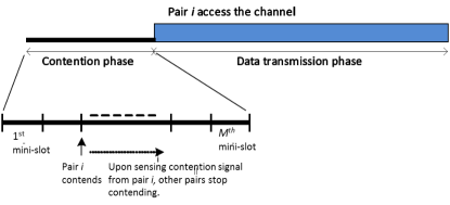
(a) Successful Contention

(b) Collision in Contention Phase

Figure 4: An illustration for the steps in Algorithm 1

Operation of CADS takes place in slotted time in two phases: (i) contention phase and (ii) data transmission phase. The contention phase is composed of $M$ mini-slots, each of which is of enough duration to detect contention signals from other edge devices, i.e., a mini-slot must be at least $8\mu\mbox{s}$ in an IEEE 802.11b environment. If $\tau$ is the ratio of the mini-slot duration to the duration of a regular time slot, then the parameter $M\tau$, which will appear below, signifies the fraction of time spent to resolve collisions.

The contention from edge devices for time slot $t\in\mathbb{N}$ is resolved as follows. The $i$th pair selects a mini-slot $m\in\left\{1,\ldots,M\right\}$ to send its contention signal. The selected mini-slot $m$ depends on the pair $i$’s weight $W_{i}(t)$ that incorporates queue backlog, direct channel and interference channel information into a single parameter. If the pair $i$ senses a contention signal from another pair before the $m$th mini-slot, it stops contending for the channel and defers its data transmission to the next time slot, i.e., ${\cal I}_{i}(t)=0$. Otherwise, it sends a contention signal in the beginning of the $m$th mini-slot. If no collision is sensed, then the $i$th pair obtains the access for the channel to transmit its data for the remaining part of the time slot, called the data transmission phase, commencing after the contention phase. If a collision is sensed, then the time slot remains idle and no data transmission takes place. These steps are visually illustrated in Fig. 4 and summarized in Algorithm 1 below.

Algorithm 1 Contention Resolution in CADS

1. At the beginning of each time slot $t\in\mathbb{N}$, the pair $i\in\left\{1,\ldots,N\right\}$ picks a mini-slot $m\in\{1,\ldots M\}$ based on its weight $W_{i}(t)$.

2. If contention signal is sensed before the $m$th mini-slot, then the pair $i$ suspends its contention by setting ${\cal I}_{i}(t)=0$.

3. If no contention signal is sensed, the pair $i$ transmits a contention signal in the beginning of the $m$th mini-slot.

- If a collision is detected, the pair $i$ sets ${\cal I}_{i}(t)=0$.

- If no collision is detected, the pair $i$ sets ${\cal I}_{i}(t)=1$, and starts its transmission in the beginning of data transmission phase.

4. The whole process restarts in the next time slot.

Based on the contention resolution phase described above, the edge pairs with the smallest backoff time have a chance of earning access rights for the channel. Hence, it is of critical importance to design an efficient association policy mapping small backoff times to the large weights $W_{i}(t)$ to ensure high utility and to exploit multiuser diversity. Our aim below is to investigate the structure of such efficient policies associating device weights with the mini-slot indices.

Definition 4

A mini-slot association policy $\boldsymbol{\Theta}\left(\boldsymbol{w}\right)=\left[\Theta_{1}\left(w_{1}\right),\ldots,\Theta_{N}\left(w_{N}\right)\right]$ is a mapping $\boldsymbol{\Theta}:\mathbb{R}_{+}^{N}\mapsto\left\{1,\ldots,M+1\right\}^{N}$ such that its $i$th component function $\Theta_{i}\left(w_{i}\right)$ determines the mini-slot index to which the $i$th pair with weight $w_{i}$ is assigned. Further, $\boldsymbol{\Theta}$ is said to be a threshold policy if all of its component functions can be written as

$$\Theta_{i}\left(w\right)=\begin{cases}m,&\text{ if }a_{m}^{(i)}\leq w<a_{m-1}^{(i)},\ \text{ for }m\in\{1,\ldots,M\}\\ M+1,&\text{ if }w<0,\end{cases}$$

where $\Theta_{i}(w)=M+1$ indicates that the edge pair $i$ does not contend for the channel in time slot $t\in\mathbb{N}$.

We note that the mini-slot index $M+1$ is introduced above for the sake of indicating that transmission from an edge pair is deferred to a next time slot if its weight is negative. In this case, transmissions from such pairs cause more harm to the core AP than its benefit by causing excessive interference. Below, we design a threshold-based mini-slot association policy in which the goal is to operate in close proximity of the optimal point without imposing high complexity as well as providing fairness between edge pairs. In Section VII, we compare the performance of the designed policy with different threshold-based mini-slot association policies that mainly differ from each other based on how they determine the threshold values.

VI-B CADS with Uniform Mapping

In CADS with uniform mapping, each edge pair is assigned to a mini-slot such that assignment instances are uniformly deployed over all available mini-slots. This is achieved by utilizing the distribution of weights $W_{i}(t)$ of edge pairs as follows. Let $F_{i,t}(w)$ be the conditional cumulative distribution function (CDF) of $W_{i}(t)$ at time slot $t\in\mathbb{N}$, defined as

$$F_{i,t}(w)=\mathsf{Pr}\left\{{W_{i}(t)\leq w|W_{i}(t)\geq 0,Q_{i}(t),Z(t)}\right\}.$$ (23)

Furthermore, let $(F_{i,t})^{-1}(\cdot)$ be the inverse function of $F_{i,t}(\cdot)$. The following lemma indicates how to select the threshold values to achieve uniform distribution over all mini-slot indices.

Lemma 1

For time-slot $t\in\mathbb{N}$, consider the mini-slot association policy $\boldsymbol{\Theta}$ defined as

$$\Theta_{i}(w)=\begin{cases}m,&\text{ if }(F_{i,t})^{-1}\left(\frac{M-m}{M}\right)\leq w<(F_{i,t})^{-1}\left(\frac{M-m+1}{M}\right)\\ &\hskip 91.04872pt\text{ for }m\in\{1,\ldots,M\}\\ M+1,&\text{ if }w<0,\end{cases}$$

for $i\in\left\{1,\ldots,N\right\}$. Then, for all $t\in\mathbb{N}$, $\boldsymbol{\Theta}$ induces a uniform distribution over mini-slot indices to assign edge pairs.

Proof:

Directly follows from threshold definitions. ∎

The mini-slot association policy above ensures that in the long term, each pair contends in each mini-slot with the same number of times, i.e., on the average with probability of $\frac{1}{M}$ given that its weight is positive. The goal here is to minimize the probability of collision by spreading the contention instances uniformly over all mini-slots. Furthermore, this mini-slot association policy also enforces the scheduling of a good edge device pair with respect to the current channel and queue states. However, it should be noted that such a uniform mapping policy, although promising, does not necessarily guarantee the scheduling of the best edge pair, i.e., the pair that has the maximum weight, as discussed subsequently.

The first performance loss in the CADS with uniform mapping is due to the contention phase during which an $M\tau$ fraction of whole time slot is used for contention resolution. The second performance loss arises from the possible collisions in the contention phase. Whenever a collision occurs, all edge pairs remain silent during the data transmission phase, and the channel becomes under-utilized. The third performance loss is the result of imperfect scheduling. The CADS with uniform mapping does not always schedule the edge pair that has the maximum weight. The main underlying reason behind this phenomenon is that each edge device is assigned to a mini-slot uniformly at random with respect to their weights. Although this provides fairness among devices in giving the access rights to the channel (i.e., devices with lower and higher weights are treated equally), it can lead to an assignment of channel access rights to the edge devices with smaller weights.

The next theorem provides an expression for the success probability in the CADS with uniform mapping.

Theorem 4

Let $S(t)$ be the event that the contention resolution phase is successful for time slot $t\in\mathbb{N}$ in the CADS with uniform mapping. Then,

$$\mathsf{Pr}\left(S(t)\right)=\sum_{k=1}^{M}\frac{N(t)}{M}\left(\frac{M-k}{M}\right)^{N(t)-1},$$

where $N(t)$ is the number of edge pairs with positive weights at time slot $t$.

Proof:

Please see Appendix B. ∎

We note that the success probability decreases with the number of contending edge users. The worst case scenario is for when $N(t)=N$. Hence, choosing $M$ large with respect to $N$ to guarantee a worst case success probability, we can increase channel utilization. In addition to $\mathsf{Pr}\left(S(t)\right)$, another important parameter to assess the efficiency of the CADS with uniform mapping is the weight of the scheduled edge pair for transmission, which is given by $\sum_{i=1}^{N}{\cal I}_{i}(t)W_{i}(t)$. Our simulation results indicate that the CADS with uniform mapping stabilizes the queue sizes around the same stationary points for all users, as expected due to fairness property. In this case, we can obtain a lower bound on the expected scheduled weight with respect to the maximum weight scheduling.

Theorem 5

Assume that the edge users observe identically distributed weights over the sample paths generated by the CADS with uniform mapping. For $M\geq N(t)$,

$${\mathsf{E}}\left[{\sum_{i=1}^{N}{\cal I}_{i}(t)W_{i}(t)}\right]\geq\alpha(t){\mathsf{E}}\left[{W_{*}(t)}\right],$$

where $\alpha(t)=\frac{1-\left(\frac{N(t)}{M}\right)^{N(t)}}{\left(1+\frac{1}{N(t)-1}\right)^{N(t)-1}}$, and $N(t)$ and $W_{*}(t)$ are the number of edge pairs with positive weights and the maximum weight at time slot $t\in\mathbb{N}$.

Proof:

Please see Appendix B. ∎

We note that this is a rather conservative lower bound on ${\mathsf{E}}\left[{\sum_{i=1}^{N}{\cal I}_{i}(t)W_{i}(t)}\right]$. One reason is that we designed it to be independent of the fading distributions and network states. It can be improved for specific distributions. This bound becomes tighter for $N(t)$ small and $M$ large. Especially, for $M\geq\left(1+\epsilon\right)N(t)$, $\epsilon>0$ and $N(t)$ large, we can write

$${\mathsf{E}}\left[{\sum_{i=1}^{N}{\cal I}_{i}(t)W_{i}(t)}\right]\geq e^{-1}{\mathsf{E}}\left[{W_{*}(t)}\right].$$

One appealing feature of Theorem 5 is that it can help us to relate the scheduled weight in the CADS with uniform mapping to the maximum weight $W^{*}(t)$ scheduling achieved by the centralized algorithm. In particular, $W_{*}(t)$ is equal to $\left(1-M\tau\right)W^{*}(t)$ whenever both centralized and distributed algorithms observe the same queue states. However, the frequency at which they hit the same states is not the same. Hence, the relationship between ${\mathsf{E}}\left[{W_{*}(t)}\right]$ and ${\mathsf{E}}\left[{W^{*}(t)}\right]$ is more involved. The following theorem provides a lower bound on the performance achieved by the CADS with uniform mapping by considering above observations.

Theorem 6

Let $\alpha^{*}=\beta\frac{1-\left(\frac{N}{M}\right)^{N}}{\left(1+\frac{1}{N-1}\right)^{N-1}}$, $\beta=\frac{{\mathsf{E}}\left[{W_{*}(t)}\right]}{{\mathsf{E}}\left[{W^{*}(t)}\right]}$ and $M\geq N$. Suppose $\boldsymbol{x^{*}}=[x_{1}^{*},\ldots,x_{N}^{*}]$ is the average arrival rates produced by the CADS with uniform mapping. Then, for any flow parameter $V>0$, the algorithm achieves the following performance bound:

$$\sum_{i=1}^{N}U_{i}(x_{i}^{*}) \geq\alpha^{*}U^{*}-\frac{B_{2}}{V}$$

while bounding the long-term expected queue lengths as:

$$\limsup_{T\rightarrow\infty}\frac{1}{T}\sum_{\tau=0}^{T-1}\sum_{i=1}^{N}{\mathsf{E}}\left[{Q_{i}(\tau)}\right] \leq\frac{B_{2}+V\kappa}{\epsilon_{3}},$$

where $B_{2},\epsilon_{3},\kappa>0$ are constants and $U^{*}$ is the optimal aggregate utility of the problem in (12)-(13).

Proof:

The proof follows from using the worst case bound in Theorem 5 and Corollary 5.2 in [10]. ∎

VII Numerical Results

In this section, we present an extensive numerical and simulation study illustrating the analytical results obtained above.

VII-A Distributed Schedulers for Performance Comparison

First, we introduce other CADS algorithms for comparing the performance of our baseline CADS algorithm, which is the CADS with uniform mapping.

VII-A1 CADS with Optimal Weight Mapping

This scheduler uses a threshold association policy that maximizes the expected weight of edge device pairs. That is to say, the sequence of threshold values $\left\{a_{m}\right\}_{m=1}^{M}$ is determined as a solution of the following optimization problem

$$\max_{\left\{a_{m}\right\}_{m=1}^{M}}\ {\mathsf{E}}\left[{{\cal I}_{i}(t)W_{i}(t)}\right]=\sum_{m=1}^{M}{\mathsf{E}}\left[{{\cal I}_{i}(t)W_{i}(t)|\Theta_{i}(W_{i}(t))=m}\right]$$

for all $i\in\left\{1,\ldots,N\right\}$. Since the above optimization problem is highly non-linear and dependent on the distributions of fading processes, we are not able to obtain a closed-form solution. Hence, we numerically solve the above problem. Since the CADS with optimal weight mapping maximizes ${\mathsf{E}}\left[{{\cal I}_{i}(t)W_{i}(t)}\right]$ for all $i\in\left\{1,\ldots,N\right\}$, it results in better performance than that obtained by the uniform mapping, albeit at the expense of increased complexity.

VII-A2 CADS with Linear Mapping

This scheduler uses an easy-to-implement and efficient algorithm for the edge devices having limited power and memory. Specifically, it utilizes a discrete linear mapping function $\Theta_{i}$ defined as

$$\Theta_{i}(w)=\begin{cases}m,&\text{ if }\frac{(M-m-1)W_{max}}{M}\leq w<\frac{(M-m)W_{max}}{M},\\ &\ \ \ \ \ \ \ \ \ \ \ \ \ \ \ \ \ \ \ \ \text{ for }m\in\{1,\ldots,M\}\\ M+1,&\text{ if }w<0,\end{cases}$$

for all $i\in\left\{1,\ldots,N\right\}$, where $W_{max}$ is a large constant representing an upper bound on the weight realizations. All edge devices agree on the value of $W_{max}$ and then use the above mapping to determine mini-slot indices.

VII-A3 Interference Regulated Distributed Scheduler

We modify the baseline algorithm proposed in [39] to obtain an interference regulated distributed scheduler (IRDS).

The operation of IRDS is divided into two phases: (i) contention phase and (ii) data transmission phase, similar to the CADS algorithms above. To facilitate the discussion, we introduce two new random variables related to contention and scheduling phases. The first one is the contention variable, $a_{i}(t)$, that is 1 with probability $\frac{1}{N}$, and 0 with probability $\frac{N-1}{N}$. The second one is the transmission variable, $p_{i}(t)$, that is 1 with probability $\frac{e^{W_{i}(t)}}{e^{W_{i}(t)}+1}$, and 0 with probability $\frac{1}{e^{W_{i}(t)}+1}$, where $W_{i}(t)$ is the weight of edge pair $i$ defined in (20) for all $i\in\left\{1,\ldots,N\right\}$. We note that the transmission variable takes also into account interference level that is caused to the core AP. This is the reason why the algorithm is regulated with respect to the interference level.

The scheduling decision of edge pair $i\in\left\{1,\ldots,N\right\}$ depends on the following three conditions:

Condition (1): The contention of pair $i$ is successful, i.e., $a_{i}(t)\prod_{j\neq i}(1-a_{j}(t))=1$.

Condition (2): None of the neighboring pairs were scheduled in the previous time slot, i.e., $\sum_{j\neq i}{\cal I}_{j}(t-1)=0$

Condition (3): The transmission variable $p_{i}(t)=1$.

Based on these three conditions, the scheduling phase consists of three different cases, as given by Algorithm 2.

Algorithm 2 Scheduling Phase of IRDS

Each edge pair determines ${\cal I}_{i}(t)$ according to

Case 1: ${\cal I}_{i}(t)=1$ if the conditions (1), (2) and (3) hold.

Case 2: If the condition (1) does not hold and the condition (3) holds, then ${\cal I}_{i}(t)={\cal I}_{i}(t-1)$.

Case 3: Otherwise, ${\cal I}_{i}(t)=0$.

Notice that the IRDS only considers a single round contention unlike the proposed CADS algorithms, which limits the edge network performance as shown in simulation results.

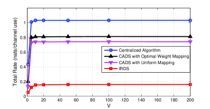
Figure 5: Performance of the edge network as a function of $V$. Both centralized and distributed dynamic control mechanisms are considered.

VII-B Simulation Results

In the simulations below, we consider iid Rayleigh fading channels, with direct and interference power gains given by exponential distributions having means $2$ and $1$, respectively. The service rate functions $R_{i}(t)$ are chosen to be $R_{i}(t)=\log\left(1+\frac{Ph_{i}(t)}{I_{i}(t)+1}\right)$ for all $i\in\left\{1,\ldots,N\right\}$. Further, we use logarithmic utility functions to measure edge device satisfaction for an achieved rate value $x_{i}$ for $i=1,\ldots,N$. Specifically, the edge pair $i$ obtains a proportionally fair utility of $\log(1+x_{i})$ at rate $x_{i}$. Since the sum of utility functions are taken as the objective function to be maximized, we obtain the utility maximizing arrival rates of edge devices, and the rates depicted in the graphs below are the sum of these optimum arrival rates. To simulate $I_{i}(t)$, we generate $20$ exponentially distributed interfering links to the edge network devices, and the mean channel gains of these links are randomly chosen between $0.1$ and $0.3$. The total interference at the $i$th edge device pair is the weighted sum of the gains of these interfering links, with weights being the transmission powers that are set to unity. Unless otherwise stated, the number of edge device links and mini-slots are set to $100$ and $200$, respectively. Furthermore, we take $\gamma=0.1$ and $\tau=10^{-4}$ except simulations conducted with respect to these parameters. We will only consider average interference constraints in the simulations below for the sake of having a clean exposition.

We compare the performance curves for CADS with uniform mapping, CADS with optimal weight mapping, CADS with linear mapping and IRDS with the performance obtained through the centralized algorithm. To start with, we investigate the effect of the system parameter $V>0$ on our dynamic control algorithms in Fig. 5. As expected, the total rate of all algorithms increases with increasing $V$ values, and Fig. 5 shows that the rate achieved by the centralized algorithm for $V\geq 20$ converges to its optimal value fairly closely verifying the results in Theorem 3.

Furthermore, the distributed algorithm achieving the best performance is the CADS with optimal weight mapping. It attains an average rate over $80\%$ of the total rate of the centralized algorithm. The CADS with uniform mapping exhibits a performance curve fairly close to the one with optimal weight mapping, achieving around $70\%$ of the total rate of the centralized algorithm. Based on the derived success probability distribution in Theorem 4, we observe that the success in the earlier mini-slots become more likely than those in the later mini-slots, which is eventually more beneficial due to higher weight scheduling. However, such collision minimization does not correspond to an optimized performance with max-weight scheduling since it is still possible that the successfully scheduled edge pair does not have the maximum weight. The first factor puts an upward pressure to increase the performance of the CADS with uniform mapping, whereas the second one puts a downward pressure to decrease the performance of the CADS with uniform mapping. At the end, they balance each other, leading to an observed slightly worse performance of the CADS with uniform mapping.

Among four distributed schedulers, the IRDS has the worst performance achieving only approximately $30\%$ of that of the centralized algorithm. There are mainly two reasons about such a poor performance for the IRDS. Firstly, the IRDS cannot fully take advantage of channel diversity due to using single contention period. It schedules an edge device randomly, and then decides whether the scheduled edge device should transmit or not after the scheduling decision. Secondly, to schedule a new edge device, the algorithm always requires an idle time-slot, and this increases the number of idle time-slots leading to under-utilization of the channel.

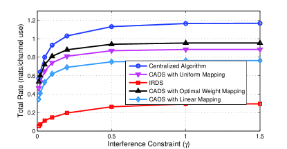
(a) Performance with respect to $\gamma$

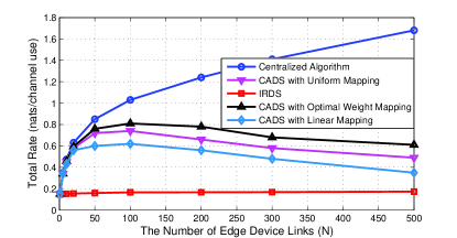
(b) Performance with respect to $N$

Figure 6: Performance of the edge network as a function of $\gamma$ and $N$. Both centralized and distributed dynamic control mechanisms are considered.

For the rest of the experiments, we take $V=100$. In Figs. 6a and 6b, we analyze the effect $\gamma$ and $N$ on the system performance, respectively. As illustrated in Fig. 6a, the total rate of all algorithms increases with increasing $\gamma$. This is because for low $\gamma$ values, in order to satisfy a tight interference constraint, a larger fraction of time-slots remains idle, i.e., smaller number of transmission opportunities are given to edge device pairs. Starting around $\gamma$ = 0.5, the interference constraint becomes inactive. In Fig. 6b, we first notice that the performance of the IRDS does not change with increasing number of pairs and only achieves $90\%$ of the rate achieved by the centralized algorithm when the number of device pairs is equal to one. This result arises from the fact that the IRDS cannot take the advantage of diversity gains available in fading channels. On the other hand, the CADS algorithms achieve performances that are closer to the centralized algorithm due to taking advantage of link diversity. As expected, the CADS with optimal weight mapping performs the best, whereas the one with linear mapping has the worst performance. In the case of linear mapping, we sacrifice some performance in favor of reducing mapping complexity. However, as $N$ increases, the collisions in contention phase become more dominant compared to diversity gain, and as $N>500$, the total rate of CADS algorithms decreases.

We should note that the performance of the CADS with linear mapping mainly depends on two factors. The first one is the selection of $W_{max}$. If $W_{max}$ is too small, then the channel access attempts get clustered around the earlier mini-slots. This results in high volume of collisions and decreases the performance of the algorithm. On the contrary, if $W_{max}$ is too large, then the edge devices tend to select later mini-slots to contend. This again causes high volume of collisions. In the light of this discussion, we select $W_{max}$ such that the worst case probability of weights being larger than $W_{max}$ is $\frac{1}{M}$. The second factor that affects the performance of the CADS with linear mapping is the shape of the CDFs of the weights. If the CDFs are closer to linear functions, then we can say that the algorithm can perform well.

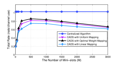
(a) $\tau=10^{-4}$

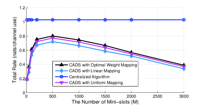
(b) $\tau=2\cdot 10^{-4}$

Figure 7: Performance of the edge network as a function of $M$. Both centralized and distributed dynamic control mechanisms are considered.

Next, we analyze the effect of the number of mini-slots on the edge network performance. In Fig. 7a, we take $\tau=10^{-4}$ and in Fig. 7b, we take $\tau=2\cdot 10^{-4}$. As illustrated in these figures, the total data rate increases initially with increasing values of $M$. This is due to the fact the edge network experiences less collisions with increasing $M$. However, when $M$ is excessively high, the emphasis on reducing collisions becomes less significant, but the loss due to the contention window size is more prominent. As a result, the performance of CADS algorithms gets worse. Furthermore, the decrease of the total rate due to having long contention phase is sharper in Fig. 7b. This is because higher $\tau$ corresponds to higher cost of implementing mini-slots, so the optimal $M$ decreases.

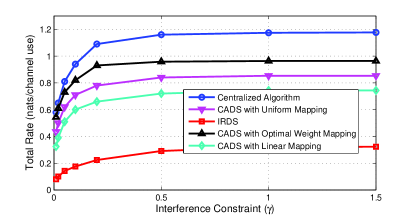
(a) Performance with respect to $\gamma$

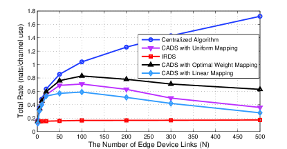
(b) Performance with respect to N

Figure 8: Performance of the edge network as a function of $\gamma$ and $N$ with non-iid channels. Both centralized and distributed dynamic control mechanisms are considered.

Lastly, we investigate the edge network performance with respect to $\gamma$ and $N$ when the channels are not iid. Precisely, the direct and interference channel gains of edge pairs are chosen uniformly at random from the intervals $\left[1.2,2.8\right]$ and $\left[0.2,1.8\right]$, respectively. The same observations above continue to hold. Differently, we notice that the CADS with uniform mapping perform slightly worse than the case when the channel gains are iid. The reason is that when the channel gains are non-iid, the difference between the weights and the queue sizes of edge devices becomes larger. Then, the CADS algorithms cannot schedule the edge pair with the highest weight more frequently due to having different mapping intervals at each pair.

VIII Conclusion

In this paper, we considered the problem of cross-layer design for underlay edge networks. We first derived the stability region for the edge network subject to interference constraints at the core AP. We then designed a cross-layer flow control and scheduling algorithm that maximizes the total collective utility of the edge network within the stability region. This is a centralized algorithm that requires knowledge of edge device queue sizes for scheduling. We also studied distributed implementation issues by relaxing the design of the centralized algorithm. The loss from distributed operation was characterized. Finally, an extensive simulation and numerical study was performed. The derived analytical results as well as the performance gap between the centralized and distributed schedulers were illustrated as a function of various edge network parameters. As a future work, we plan to investigate the performance of interference-aware mobile edge network in a multi-user scheduling setting where a number of edge devices can transmit in the same time-slot.

Appendix A Proof of Theorem 1

Assume that the primal optimization problem in (5)-(8) is feasible with an interior point. Let $\Omega\subseteq\Psi$ contain all scheduling policies satisfying $\sum_{i=1}^{N}{\cal I}_{i}\left(\boldsymbol{h},\boldsymbol{g},\boldsymbol{I}\right)\leq 1$ and ${\cal I}_{i}\left(\boldsymbol{h},\boldsymbol{g},\boldsymbol{I}\right)=0$ if $Pg_{i}>\nu$ for all fading and interference states. Then, the primal problem can be recast as

$$\begin{array}[]{ll}\mbox{maximize}_{\boldsymbol{\cal I}\in\Omega}&{\mathsf{E}}\left[{{\cal I}_{i}(\boldsymbol{h},\boldsymbol{g},\boldsymbol{I})R_{i}}\right]\\ \mbox{subject to}&{\mathsf{E}}\left[{{\cal I}_{j}(\boldsymbol{h},\boldsymbol{g},\boldsymbol{I})R_{j}}\right]\geq\alpha_{j},\forall j\neq i\\ &{\mathsf{E}}\left[{\sum_{j=1}^{N}P{\cal I}_{j}(\boldsymbol{h},\boldsymbol{g},\boldsymbol{I})g_{j}}\right]\leq\gamma\end{array}.$$ (27)

Consider the Lagrangian for the above problem defined as

$$L\left(\boldsymbol{\cal I},\boldsymbol{\lambda},\mu\right)={\mathsf{E}}\left[{{\cal I}_{i}(\boldsymbol{h},\boldsymbol{g},\boldsymbol{I})R_{i}}\right]+\sum_{j\neq i}\lambda_{j}\left({\mathsf{E}}\left[{{\cal I}_{j}(\boldsymbol{h},\boldsymbol{g},\boldsymbol{I})R_{j}}\right]-\alpha_{j}\right)$$

$$+\mu\left(\gamma-\sum_{j=1}^{N}{\mathsf{E}}\left[{P{\cal I}_{j}(\boldsymbol{h},\boldsymbol{g},\boldsymbol{I})g_{j}}\right]\right),$$

where $\mu\geq 0$ and $\boldsymbol{\lambda}\in\mathbb{R}_{+}^{N-1}$ are associated Lagrange multipliers [40]. We observe that the set $\Omega$ is convex in the sense that if $\boldsymbol{\cal I}_{1}\in\Omega$ and $\boldsymbol{\cal I}_{2}\in\Omega$, then $a\boldsymbol{\cal I}_{1}+\left(1-a\right)\boldsymbol{\cal I}_{2}$ also lies in $\Omega$. Hence, there exists $\mu^{*}$ and $\boldsymbol{\lambda}^{*}$ such that the optimal value of the following convex problem

$$\max_{\boldsymbol{\cal I}\in\Omega}L\left(\boldsymbol{\cal I},\boldsymbol{\lambda}^{*},\mu^{*}\right)$$ (28)

coincides with the optimal value of the primal problem [40]. This problem is easy to solve since the constraints defining $\Omega$ are given for each state. Therefore, (28) can be solved for each fading and interference state, which leads to

$${\cal I}^{*}_{j}\left(\boldsymbol{h},\boldsymbol{g},\boldsymbol{I}\right)=\left\{\begin{IEEEeqnarraybox}[]{[}][c]{l^{\prime}s}1,&if$j \in\operatorname*{argmax}_{k \in C} W_k$\\ 0,&otherwise\end{IEEEeqnarraybox}\right.$$ (31)

for all $j\in\left\{1,\ldots,N\right\}$, where $C=\left\{j:Pg_{j}\leq\nu\mbox{ and }W_{j}\geq 0\right\}$ and $W_{j}$ is given by $W_{j}=\lambda_{j}^{*}R_{j}-\mu^{*}Pg_{j}$ for $j\neq i$ and $W_{i}=R_{i}-\mu^{*}Pg_{i}$. It also holds that any solution for (27) is also a solution for (28). This concludes the proof since the above solution given in (31) is unique almost surely.

Appendix B Performance of the CADS with Uniform Mapping

B-A Proof of Theorem 4

Assume there are $N(t)$ edge pairs with positive weights at time slot $t\in\mathbb{N}$. Without loss of generality, label them as $W_{i}$ for $i=1,\ldots,N(t)$. Let $m_{i}=\Theta\left(W_{i}\right)$ and $m^{*}=\min_{1\leq i\leq N(t)}m_{i}$. Observe that $m^{*}$ is the minimum of $N(t)$ uniformly and independently distributed random variables over $\left\{1,\ldots,M\right\}$. Then,

$$\mathsf{Pr}\left(S(t)\mbox{ and }m^{*}=m\right)=\frac{N(t)}{M}\left(\frac{M-m}{M}\right)^{N(t)-1}$$

since at least one edge pair must be assigned to the mini-slot $m$ and the rest must be assigned to those with higher indices for both $S(t)$ and $m^{*}=m$ to hold correct. Summing over $m$, we obtain $\mathsf{Pr}\left(S(t)\right)$ as stated in the theorem.

B-B Proof of Theorem 5

Let $\mathcal{F}_{t}$ be the $\sigma$-algebra generated by the states $\left\{Q_{i}(t)\right\}_{i=1}^{N}$ and $Z(t)$. Using the same notation above, let $W_{*}(t)=\max_{1\leq i\leq N(t)}W_{i}$. Observe that we always have $\sum_{i=1}^{N}{\cal I}_{i}(t)W_{i}(t)=W_{*}(t)$ on the event $S$. Then,

$${\mathsf{E}}\left[{\sum_{i=1}^{N}{\cal I}_{i}(t)W_{i}(t)\Big{|}\mathcal{F}_{t}}\right] = {\mathsf{E}}\left[{\sum_{i=1}^{N}{\cal I}_{i}(t)W_{i}(t);S(t)\Big{|}\mathcal{F}_{t}}\right]$$

$$= {\mathsf{E}}\left[{W_{*}(t);S(t)\big{|}\mathcal{F}_{t}}\right],$$

where ${\mathsf{E}}\left[{\sum_{i=1}^{N}{\cal I}_{i}(t)W_{i}(t);S(t)\big{|}\mathcal{F}_{t}}\right]$ indicates the expectation of the random variable $\sum_{i=1}^{N}{\cal I}_{i}(t)W_{i}(t)$ on the event $S(t)$. The next lemma provides an expression for ${\mathsf{E}}\left[{W_{*}(t);S(t)\big{|}\mathcal{F}_{t}}\right]$.

Lemma 2

$${\mathsf{E}}\left[{W_{*}(t);S(t)\big{|}\mathcal{F}_{t}}\right]\hskip 227.62204pt$$

$$=N(t)\sum_{m=1}^{M}\left(\frac{M-m}{M}\right)^{N(t)-1}{\mathsf{E}}\left[{W;a_{m}\leq W<a_{m-1}\big{|}\mathcal{F}_{t}}\right],\hskip 48.36958pt$$

$W$ is a generic random variable having the same conditional distributions with $W_{i}$’s and $a_{m}$’s are the associated threshold values in the CADS with uniform mapping.

Proof:

Let $E_{i}$ be the event that $m_{i}=m$ and $m_{j}>m$ for all $j\neq i$. Then, we can write

$${\mathsf{E}}\left[{W_{*}(t);S(t)\big{|}\mathcal{F}_{t}}\right] = \sum_{m=1}^{M}{\mathsf{E}}\left[{W_{*}(t);S(t),m^{*}=m\big{|}\mathcal{F}_{t}}\right]$$

$$= \sum_{m=1}^{M}\sum_{i=1}^{N(t)}{\mathsf{E}}\left[{W_{*}(t);E_{i}\big{|}\mathcal{F}_{t}}\right]$$

$$= \sum_{m=1}^{M}\sum_{i=1}^{N(t)}{\mathsf{E}}\left[{W_{*}(t)\big{|}E_{i},\mathcal{F}_{t}}\right]\mathsf{Pr}\left(E_{i}\big{|}\mathcal{F}_{t}\right)$$

$$= \sum_{m=1}^{M}\sum_{i=1}^{N(t)}{\mathsf{E}}\left[{W_{i}\big{|}E_{i},\mathcal{F}_{t}}\right]\mathsf{Pr}\left(E_{i}\big{|}\mathcal{F}_{t}\right).$$

Since the weights are assumed to be conditionally iid, we have ${\mathsf{E}}\left[{W_{i}\big{|}E_{i},\mathcal{F}_{t}}\right]=M{\mathsf{E}}\left[{W;a_{m}\leq W<a_{m-1}\big{|}\mathcal{F}_{t}}\right]$. Further, $\mathsf{Pr}\left(E_{i}\big{|}\mathcal{F}_{t}\right)=\frac{1}{M}\left(\frac{M-m}{M}\right)^{N(t)-1}$. Combining these results, we complete the proof of Lemma 2. ∎

Now, we will bound ${\mathsf{E}}\left[{W_{*}(t)\big{|}\mathcal{F}_{t}}\right]$. First observe that

$${\mathsf{E}}\left[{W_{*}(t)\big{|}\mathcal{F}_{t}}\right] = \sum_{m=1}^{M}\int_{a_{m}}^{a_{m-1}}N(t)f_{W}(w)\left(F_{W}(w)\right)^{N(t)-1}dw$$

$$\leq N(t)\sum_{m=1}^{M}\left(\frac{M-m+1}{M}\right)^{N(t)-1}$$

$$\hskip 51.21504pt\times{\mathsf{E}}\left[{W;a_{m}\leq W<a_{m-1}\big{|}\mathcal{F}_{t}}\right],$$

where $f(w)$ and $F(w)$ are the conditional PDF and CDF for $W$, respectively. Dividing above sum into two parts, we obtain

$${\mathsf{E}}\left[{W_{*}(t)\big{|}\mathcal{F}_{t}}\right]\left(1-N(t)\sum_{m=1}^{N(t)-1}\left(\frac{m}{M}\right)^{N(t)-1}\right)\hskip 227.62204pt$$

$$\leq N(t)\sum_{m=1}^{M-N(t)+1}\left(\frac{M-m+1}{M}\right)^{N(t)-1}{\mathsf{E}}\left[{W;a_{m}\leq W<a_{m-1}\big{|}\mathcal{F}_{t}}\right].\hskip 136.5733pt$$

Now, we compare the terms $\left(\frac{M-m+1}{M}\right)^{N(t)-1}$ and $\left(\frac{M-m}{M}\right)^{N(t)-1}$. The ratio of these two terms is bounded above by $\left(\frac{M-m+1}{M-m}\right)^{N(t)-1}\leq\left(1+\frac{1}{M-m}\right)^{N(t)-1}\leq\left(1+\frac{1}{N(t)-1}\right)^{N(t)-1}$. Using Lemma 2, this shows that

$${\mathsf{E}}\left[{W_{*}(t)\big{|}\mathcal{F}_{t}}\right]\left(1-N(t)\sum_{m=1}^{N(t)-1}\left(\frac{m}{M}\right)^{N(t)-1}\right)\hskip 227.62204pt$$

$$\leq\left(1+\frac{1}{N(t)-1}\right)^{N(t)-1}{\mathsf{E}}\left[{W_{*}(t);S(t)\big{|}\mathcal{F}_{t}}\right].\hskip 156.49014pt$$

The above sum can be bounded above by $\frac{1}{N(t)}\left(\frac{N(t)}{M}\right)^{N(t)}$. Hence, the following bound holds

$${\mathsf{E}}\left[{W_{*}(t);S(t)\big{|}\mathcal{F}_{t}}\right]\geq\frac{1-\left(\frac{N(t)}{M}\right)^{N(t)}}{\left(1+\frac{1}{N(t)-1}\right)^{N(t)-1}}{\mathsf{E}}\left[{W_{*}(t)\big{|}\mathcal{F}_{t}}\right].$$

Averaging over $\mathcal{F}_{t}$, we finally have

$${\mathsf{E}}\left[{W_{*}(t);S(t)}\right]\geq\frac{1-\left(\frac{N(t)}{M}\right)^{N(t)}}{\left(1+\frac{1}{N(t)-1}\right)^{N(t)-1}}{\mathsf{E}}\left[{W_{*}(t)}\right],$$

which completes the proof.

References

- [1] Cisco, “Cisco Visual Networking Index: Global Mobile Data Traffic Forecast, 2015-2020,” White Paper, Jan. 2016.
- [2] M. Chiang and T. Zhang, “Fog and IoT: An overview of research opportunities,” IEEE Internet Things J., to appear.
- [3] R. Kelly, “Internet of things data to top 1.6 zettabytes by 2020,” Campus Technology, Accessed on Dec. 9, 2016. [Online]. Available: https://campustechnology.com/articles/2015/04/15/internet-of-things-data-to-top-1-6-zettabytes-by-2020.aspx.
- [4] L. Mearian, “Self-driving cars could create 1GB of data a second,” Computer World, Accessed on Dec. 9, 2016. [Online]. Available: http://www.computerworld.com/article/2484219/emerging-technology/self-driving-cars-could-create-1gb-of-data-a-second.html.
- [5] I. F. Akyildiz, S. Nie, S.-C. Lin, and M. Chandrasekaran, “5G roadmap: 10 key enabling technologies,” Computer Netw., vol. 106, pp. 17–48, Sep. 2016.
- [6] M. N. Tehrani, M. Uysal, and H. Yanikomeroglu, “Device-to-device communication in 5G cellular networks: Challenges, solutions, and future research directions,” IEEE Commun. Mag., vol. 52, no. 5, pp. 86–92, May 2014.
- [7] L. Lei, Z. Zhong, C. Lin, and X. Shen, “Operator controlled device-to-device communications in LTE-advanced networks,” IEEE Wireless Commun. Mag., vol. 19, no. 3, pp. 96–104, Jun. 2012.
- [8] G. Fodor, E. Dahlman, G. Mildh, S. Parkvall, N. Reider, G. Miklos, and Z. Turanyi, “Design aspects of network assisted device-to-device communications,” IEEE Commun. Mag., vol. 50, no. 3, pp. 170–177, Mar. 2012.
- [9] A. Goldsmith, S. A. Jafar, I. Maric, and S. Srinivasa, “Breaking spectrum gridlock with cognitive radios: An information theoretic perspective,” Proc. IEEE, vol. 97, no. 5, pp. 894––914, May 2009.
- [10] L. Georgiadis, M. J. Neely, and L. Tassiulas, “Resource allocation and cross-layer control in wireless networks,” Foundations and Trends in Networking, vol. 1, no. 1, 2006.
- [11] F. P. Kelly, A. K. Maulloo, and D. K. H. Tan, “Rate control for communication networks: Shadow prices, proportional fairness and stability,” The Journal of the Operational Research Society, vol. 49, no. 3, pp. 237–252, 1998. [Online]. Available: http://dx.doi.org/10.2307/3010473
- [12] X. Wang and K. Kar, “Cross-layer rate control for end-to-end proportional fairness in wireless networks with random access,” in Proc. the Sixth ACM International Symposium on Mobile Ad Hoc Networking and Computing (MobiHoc 2005), Urbana-Champaign, IL, 2005, pp. 157–168.
- [13] C. H. Yu, O. Tirkkonen, K. Doppler, and C. B. Ribeiro, “On the performance of device-to-device underlay communication with simple power control,” in Proc. IEEE Vehicular Technology Conf. (VTC), Barcelona, Spain, Apr. 2009, pp. 1––5.
- [14] C. H. Yu, K. Doppler, C. Riberio, and O. Tirkkonen, “Resource sharing optimization for device-to-device communication underlaying cellular communication,” IEEE Trans. Wireless Commun., vol. 10, no. 8, pp. 2752–2763, Aug.
- [15] P. Janis, C. Yu, K. Doppler, C. Ribeiro, C. Wijting, K. Hugl, O. Tirkkonen, and V. Koivunen, “Device-to-device communication underlaying cellular communications system,” IEEE Trans. Inf. Theory, vol. 2, no. 3, pp. 169–178, Mar. 2009.
- [16] H. Min, J. Lee, S. Park, and D. Hong, “Capacity enhancement using an interference limited area for device-to-device uplink underlaying cellular networks,” IEEE Trans. Wireless Commun., vol. 10, no. 12, pp. 3995–4000, Dec. 2011.
- [17] X. Xiao, X. Tao, and J. Lu, “A QoS-aware power optimization scheme in OFDMA systems with integrated device-to-device (D2D) communications,” in Proc. IEEE Vehicular Technology Conf. (VTC), San Francisco, CA, 2011, pp. 1–5.
- [18] S. Hakola, T. Chen, J. Lehtomaki, and T. Koskela, “Device-to-device (D2D) communication in cellular network-performance analysis of optimum and practical communication mode selection,” in Proc. of IEEE Wireless Commun. and Netw. Conf., Sydney, Australia, Apr. 2010, pp. 1–6.
- [19] M. Jung, K. Hwang, and S. Choi, “Joint mode selection and power allocation scheme for power-efficient device-to-device (D2D) communication,” in Proc. of IEEE Vehicular Technology Conf., Yokohama, Japan, May 2012, pp. 1–5.
- [20] D. Feng, L. Lu, Y. Y.-Wu, G. Y. Li, G. Feng, and S. Li, “Device-to-device communications underlaying cellular networks,” IEEE Trans. Commun., vol. 61, no. 8, pp. 3541–3551, Aug. 2013.
- [21] L. Su, Y. Ji, P. Wang, and F. Liu, “Resource allocation using particle swarm optimization for D2D communication underlay of cellular networks,” in Proc. of IEEE Wireless Commun. and Netw. Conf., Shanghai, China, Apr. 2013, pp. 129–133.
- [22] L. B. Le, “Fair resource allocation for device-to-device communications in wireless cellular networks,” in Proc. of 2012 IEEE Global Commun. Conf., Anaheim, CA, Dec. 2012, pp. 5451––5456.
- [23] S. Gitzenis, G. S. Paschos, and L. Tassiulas, “Asymptotic laws for joint content replication and delivery in wireless networks,” vol. 59, no. 5, pp. 2760–2776, 2013.
- [24] M. Ji, G. Caire, and A. F. Molisch, “Wireless device-to-device caching networks: Basic principles and system performance,” vol. 34, no. 1, pp. 176–189, 2016.
- [25] E. Nekouei, H. Inaltekin, and S. Dey, “Throughput scaling in cognitive multiple access with average power and interference constraints,” IEEE Trans. Signal Process., vol. 60, no. 2, pp. 927–946, Feb. 2012.
- [26] E. Nekouei, H. Inaltekin and S. Dey, “Power control and asymptotic throughput analysis for the distributed cognitive uplink,” IEEE Trans. Commun., vol. 62, no. 1, pp. 41–58, Jan. 2014.
- [27] E. Nekouei, H. Inaltekin, and S. Dey, “Throughput analysis for the cognitive uplink under limited primary cooperation,” IEEE Trans. Commun., vol. 64, no. 7, pp. 2780–2796, Jul. 2016.
- [28] H. Tran, T. Q. Duong, and H. J. Zepernick, “Queuing analysis for cognitive radio networks under peak interference power constraint,” in Proc. Int. Symposium on Wireless and Pervasive Computing, Hong Kong, China, Feb. 2011, pp. 1–5.
- [29] C. Kabiri, H. Tran, and H. J. Zepernick, “Outage probability and ergodic capacity of underlay cognitive radio systems with adaptive power transmission,” in Proc. 9th Int. Wireless Commun. and Mobile Comp. Conf., Sardinia, Italy, Jul. 2013, pp. 785–790.
- [30] R. Urgaonkar and M. J. Neely, “Opportunistic scheduling with reliability guarantees in cognitive radio networks,” IEEE Trans. Mob. Comput., vol. 8, no. 6, pp. 766–777, Jun. 2009.
- [31] I. Krikidis, N. Devroye, and J. Thompson, “Stability analysis for cognitive radio with multi-access primary transmission,” IEEE Trans. Wireless Commun., vol. 9, no. 1, pp. 72––77, Jan. 2010.
- [32] L. Wang and V. Fodor, “Dynamic cooperative secondary access in hierarchical spectrum sharing networks,” IEEE Trans. Wireless Commun., vol. 13, no. 11, pp. 6068––6080, Nov. 2014.
- [33] S. Kompella, G. Nguyen, C. Kam, J. Wieselthier, and A. Ephremides, “Cooperation in cognitive underlay networks: Stable throughput tradeoffs,” IEEE/ACM Trans. Netw., vol. 22, no. 6, pp. 1756––1768, Dec. 2014.
- [34] M. Ashour, A. Elsherif, T. Elbatt, and A. Mohamed, “Cognitive radio networks with probabilistic relaying: Stable throughput and delay tradeoffs,” IEEE Trans. Commun, vol. 63, no. 11, pp. 4002––4014, Nov. 2015.
- [35] M. J. Neely, “Optimal energy and delay tradeoffs for multi-user wireless downlinks,” Tech. Rep. CSI-05-06-01, University of Southern California, 2005.
- [36] S. Boyd and L. Vandenberghe, Convex Optimization. New York, NY: Cambridge University Press, 2004.
- [37] Y. Sarikaya, H. Inaltekin, T. Alpcan, and J. Evans, “Stability and Dynamic control of Underlay Mobile Edge Networks,” Technical Report, The University of Melbourne, 2016, [Online]. Available: http://arxiv.org/abs/1606.00534.
- [38] A. W. Vaart, Asymptotic Statistics. Cambridge, UK: Cambridge University Press, 1998.
- [39] D. Xue and E. Ekici, “Efficient distributed scheduling in cognitive radio networks in the many-channel regime,” in Proc. 11th International Symposium and Workshops on Modeling and Optimization in Mobile, Ad Hoc and Wireless Networks, Tsukuba Science City, Japan, May 2013, pp. 178–185.
- [40] D. G. Luenberger, Optimization by Vector Space Methods. New York, NY: John Wiley & Sons, Inc., 1969.