Feed-forward Uncertainty Propagation in Belief and Neural Networks

Abstract

We propose a feed-forward inference method applicable to belief and neural networks. In a belief network, the method estimates an approximate factorized posterior of all hidden units given the input. In neural networks the method propagates uncertainty of the input through all the layers. In neural networks with injected noise, the method analytically takes into account uncertainties resulting from this noise. Such feed-forward analytic propagation is differentiable in parameters and can be trained end-to-end. Compared to standard NN, which can be viewed as propagating only the means, we propagate the mean and variance. The method can be useful in all scenarios that require knowledge of the neuron statistics, e.g. when dealing with uncertain inputs, considering sigmoid activations as probabilities of Bernoulli units, training the models regularized by injected noise (dropout) or estimating activation statistics over the dataset (as needed for normalization methods). In the experiments we show the possible utility of the method in all these tasks as well as its current limitations.

1 Introduction

In this work we join ideas from graphical models and mainstream NNs and present a feed-forward propagation that one one hand corresponds to an approximate Bayesian inference and on the other is trainable end-to-end. A today’s popular view is that statistical and Bayesian methods are not needed and that discriminative end-to-end training is completely sufficient. Let us therefore give examples of problems where statistical tasks arise in NNs.

One important case is when the input is noisy or has some components missing. For many sensors the noise level is known or confidences per measurement are provided (e.g., LIDAR, computational sensors). Also, not all values may be observable all the time (e.g., depth sensors). In Fig. 1 we illustrate the point that the average of the network output under noisy input differs from propagating the clean input. Taking into account the uncertainty of the input, an uncertainty of the output can be estimated and used for further processing. In classification networks, propagating the uncertainty of the input can impact the confidence of the classifier and its robustness [2]. Ideally, we would like that a classifier is not 99.99% confident when making errors, however such high confidences of wrong predictions are actually observed in NNs [22, 6, 34, 25, 29].

Another example is training with dropout [33]. Randomly deactivating neurons can be viewed as multiplicative Bernoulli noise. At the training time, the noise is sampled, so that the learning objective is the expectation of the loss over the noise and the training dataset. However, at test time, the noisy units are replaced by their expected values. Better approximating the expected value of the output may result in a faster training and better test-time performance [35].

Another example is the popular interpretation of sigmoid activations in NNs as probabilities of part detectors and of the whole NN as a hierarchy of such part detectors. If this interpretation is adopted, each inner layer has to deal with its uncertain input defined by the activation probabilities. Considering all hidden units as Bernoulli random variables, we arrive at a sigmoid belief network [24]. With respect to this model one may ask the question whether a specific value computed by the NN indeed represents some probability and how accurate it is. Without a probabilistic model such questions cannot be posed and the probabilistic interpretation becomes purely speculative.

Yet another example is computing expectations of neuron activations when the inputs range over the whole training dataset. It may turn out that the inputs to some non-linearity are always in its saturating part for the whole dataset due to the accumulated bias, or collapse to a single point due to accumulated scaling. Such statistics are crucial in initializing and normalizing NNs [11]. Analytic estimates in networks with random weights were shown to predict well the training and test performance [31].

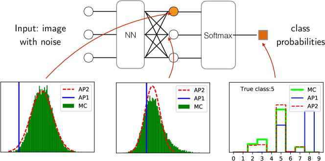
Figure 1: Illustrative example of propagating an input perturbed with Gaussian noise $\mathcal{N}(0,0.1)$ through a fully trained LeNet. When the same image is perturbed with different samples of noise, we observe on the output empirical distributions shown as MC histograms. Propagating the clean image results in the estimate denoted AP1 which may be away from the MC mean. Propagating mean and variance, as proposed in this paper, results in a posterior Gaussian distribution denoted by AP2 which approximates MC distribution better. For the final class probabilities we approximate the expected value of the softmax. A quantitative evaluation of this case is given in § 4.

To address the above statistical tasks in NNs we will use Bayesian networks, which are well-established models for reasoning with uncertainty. Let us be more precise. Bayesian, a.k.a. belief, networks are composed of random variables $X^{k}$, each variable being conditionally dependent on its parents through $p(X^{k}\,|\,X^{\operatorname{pa}(k)})$. A special case is a sigmoid belief network [24] in which random variables are binary-valued and $p(X^{k}{=1}\,|\,X^{\operatorname{pa}(k)})=\mathcal{S}({w^{k}}^{\mathsf{T}}X^{\operatorname{pa}(k)})$, where $\mathcal{S}$ is the logistic sigmoid function. A typical Bayesian inference problem consists in determining the posterior distribution of variables of interest given the values of input variables. It implies computing the expectation over all hidden random variables. This marginalization takes into account the uncertainty of all the intermediate hidden variables, but is intractable to compute in general. Neural networks, on the other hand, are composite nonlinear mappings of the form $z^{k}\,{=}\,f^{k}({w^{k}}^{\mathsf{T}}\hskip-2.15277ptz^{\operatorname{pa}(k)})$, where $z$ are continuous non-random variables and the activation functions $f^{k}$ are deterministic. The following connection with sigmoid belief networks exists [5, 7]. In the Bayesian inference problem let us approximate the expectation $\mathbb{E}[\mathcal{S}({w^{k}}^{\mathsf{T}}X^{\operatorname{pa}(k)})]$ with $\mathcal{S}({w^{k}}^{\mathsf{T}}\mathbb{E}[X^{\operatorname{pa}(k)}])$, i.e., substituting the expectation into the activation function and assuming that the variables $X^{\operatorname{pa}(k)}$ are independent. Associating the neural network variables $z^{k}$ with means $\mathbb{E}[X^{k}]$, we obtain the standard forward propagation in a neural network with sigmoid activation functions. While there exist more elaborate inference methods for belief networks (variational, mean field, Gibbs sampling, etc.), they are computationally demanding and can hardly be applied on the same scale as state-of-the-art NNs.

Contribution

Our theoretical contribution is the derivation of a feed-forward propagation method for the inference problem in Bayesian networks, connecting the methods developed for graphical models (such as belief propagation) and methods developed for neural networks. Starting from the inference problem formulation, we derive a method that propagates means and variances of all random variables through each consecutive layer. Similar propagation rules were proposed before in a more narrow context [2, 35].

Our technical contribution includes the development of numerically suitable approximations for propagating means and variances for activation functions such as sigmoid, ReLU, max and, importantly, softmax that makes the whole framework practically operational and applicable to a wider class of problems. These technical details are important but postponed to the appendix in the sake of clarity.

The proposed uncertainty propagation enjoys the following useful properties. The model is continuously differentiable even with discontinuous activation functions such as the Heaviside step function, provided that there is some uncertainty. It automatically smoothes out nonlinearities of more uncertain units, allowing better gradient propagation. It takes into account all injected noises, such as dropout, analytically (as opposed to sampling these noises), which is useful both at training and test time. It provides cheaper estimates of statistics over the dataset, can improve training speed, generalization and stability of NNs.

Experimentally, we verify the accuracy of the proposed propagation in approximating the Bayesian posterior and compare it to the standard propagation by NN, which has not been questioned before. This verification shows that the proposed scheme has better accuracy than standard propagation in all tested scenarios. We identify cases where the model scales well and cases in which it has limitations and demonstrate its potential utility in end-to-end learning.

2 Related Work

Uncertainty propagation through a multilayer perceptron [2] has been considered in a limited setting for improving robustness in speech recognition under inputs perturbed with Gaussian noise. A rather general framework of propagating means and variances was proposed under the name fast dropout training [35]. A similar feed-forward propagation using Gaussian posterior approximations was proposed as a part of probabilistic backpropagation [10]. W.r.t. these methods ours is a significant extension. We make a connection to Bayesian inference, derive refined approximations, evaluate approximation accuracy and demonstrate a wider range of applications. Another important extension is an analytic propagation through the softmax layer.

Variational inference in nonlinear Gaussian belief networks [8] uses a factorized approximation of the posterior and involves computing means and variances of activation functions such as ReLU. These components are similar to our work but the inference and learning methods are different. The relationship between Bayesian networks and NNs in the context of variational inference has been recently studied in [15]. These connections are further detailed in § 0.B.2. Our method is also related to expectation propagation in belief networks [21] and loopy belief propagation [27]. Expectation propagation is derived using forward KL divergence (similar to this work) and was shown equivalent [21] to belief propagation. These methods are iterative and to our knowledge have not been applied to NNs.

Stochastic back-propagation methods [36, 3, 28] build estimators of the gradient in a network by using samples of noise at the training time and standard propagation at test time. We estimate marginal probabilities in the stochastic network both at training and test time analytically. Analytic estimates of statistics of hidden units for purposes related to initialization and normalization occurs in [17, 1, 31] under the assumption that weights are randomly distributed, which we do not make. The proposed method may be also relevant in the context of Bayesian model estimation, i.e., inferring the posterior over the parameters given the data [19, 14, 10].

3 The Method

We consider a Bayesian network organized by layers. There are $l$ layers of hidden random variables $X^{k}$, $k=1,\dots l$ and $X^{0}$ is the input layer. Each variable $X^{k}$ has $n_{k}$ components (units in layer) denoted $X^{k}_{i}$. A conditional Bayesian network (aka belief network) is defined by the pdf

$$p(X^{1,\dots l}\,|\,X^{0})=\textstyle\prod_{k=1}^{l}\prod_{i=1}^{n_{k}}p(X^{k}_{i}\,|\,X^{k-1}).$$ (1)

The neural network can be seen as a special case of this model by writing mappings such as $Y=f(X)$ as a conditional probability $p(Y\,|\,X)=\delta(Y-f(X))$, where $\delta$ is the Dirac delta function. We will further denote values of r.v. $X^{k}$ by $x^{k}$, so that the event $X^{k}\,{=}\,x^{k}$ can be unambiguously denoted just by $x^{k}$.

3.1 Feed-forward Approximate Inference

In the Bayesian Network (1), the posterior distribution of each layer $k>1$ given the observations $x^{0}$ recurrently expresses as

$$p(X^{k}\,|\,x^{0})=\mathbb{E}_{X^{k-1}|\,x^{0}\,}\big{[}p(X^{k}\,|\,X^{k-1})\big{]}=\int p(X^{k}\,|\,x^{k-1})p(x^{k-1}\,|\,x^{0})\,dx^{k-1}.$$ (2)

The posterior distribution of the last layer, $p(X^{l}\,|\,x^{0})$ is the prediction of the model.

In general, the expectation (2) is intractable to compute and the resulting posterior can have a combinatorial number of modes. However, in many cases of interest it might be sufficient to consider a factorized approximation of the posterior $p(X^{k}\,|\,x^{0})\approx q(X^{k})=\prod_{i}q(X^{k}_{i})$. We expect that in many recognition problems, given the input image, the hidden states and the final prediction are concentrated around some specific values (unlike in generative problems, where the posterior distributions are typically multi-modal). The best approximation in terms of forward KL divergence $KL(p(X^{k}\,|\,x^{0})\|q(X^{k}))$ is given by the marginals: $q(X^{k}_{i})=p(X^{k}_{i}\,|\,x^{0})$, a well-known property explained in § 0.A for completeness.

The factorized approximation can be computed layer-by-layer, assuming that marginals of the previous layer were already approximated. Plugging the approximation $q(X^{k-1})$ in place of $p(X^{k-1}\,|\,x^{0})$ in (2) results in the procedure

$$q(X^{k}_{i})=\mathbb{E}_{q(X^{k-1})}\big{[}p(X^{k}_{i}\,|\,X^{k-1})\big{]}=\int p(X^{k}_{i}\,|\,x^{k-1})\prod_{i}q(x^{k-1}_{i})\,dx^{k-1}.$$ (3)

This expectation may be still difficult to compute exactly and we will consider suitable approximations later on.

Let us now show how these updates lead to propagation of moments. For binary variables $X^{k}_{i}$, occurring in sigmoid belief networks, the distribution $q(X^{k}_{i})$ is fully described by one parameter, e.g., the mean $\mu_{i}=\mathbb{E}_{q(X^{k}_{i})}[X^{k}_{i}]=q(X^{k}_{i}{=}1)$. The propagation rule (3) becomes

$$\mu_{i}=\mathbb{E}_{q(X^{k-1})}\big{[}p(X^{k}_{i}{=}1\,|\,X^{k-1})\big{]};\ \ \ \ \ \ \ \sigma_{i}^{2}=\mu_{i}(1-\mu_{i}),$$ (4)

where the variance is dependent but will be needed in propagation through other layers. For a continuous variable $X^{k}_{i}$, we approximate the posterior with a Gaussian distribution $q(X^{k}_{i})$. The closest approximation to the true posterior by a Gaussian distribution $\mathcal{N}(\mu_{i},\sigma_{i}^{2})$ w.r.t. forward KL divergence is given by matching the moments (also detailed in § 0.A):

$$\mu_{i} =\textstyle\int y\,\mathbb{E}_{q(X^{k-1})}[p(X^{k}_{i}\,{=}\,y\,|\,X^{k-1})]\,dy;$$ (5a)

$$\sigma_{i}^{2} =\textstyle\int y^{2}\,\mathbb{E}_{q(X^{k-1})}[p(X^{k}_{i}\,{=}\,y\,|\,X^{k-1})]\,dy-\mu_{i}^{2}.$$ (5b)

When $p(X^{k}\,|\,X^{k-1})$ takes the form of a deterministic mapping $X^{k}=f(X^{k-1})$ as in neural networks, these moments simplify to

$$\mu_{i}=\mathbb{E}_{q(X^{k})}[f(X^{k})];\ \ \ \ \ \ \ \sigma_{i}^{2}=\mathbb{E}_{q(X^{k})}[f^{2}(X^{k})]-\mu_{i}^{2}.$$ (6)

We can therefore represent the approximate inference in networks with binary and continuous variables as a feed-forward moment propagation: given the approximate moments of $X^{k-1}\,|\,x^{0}$, the moments of $X^{k}_{i}\,|\,x^{0}$ are estimated via (4), (5) ignoring dependencies between $X^{k-1}_{j}\,|\,x^{0}$ on each step (as implied by the factorized approximation). In the case of categorical variables occurring on the output of classification networks, we consider the full discrete distribution $q(X^{k})$. This case cannot be viewed as propagating moments and is treated separately.

3.2 Propagation in CNNs

Linear Layers

The statistics of a linear transform $Y=w^{\mathsf{T}}X$ are given by

$$\mu^{\prime} =\mathbb{E}[Y]=w^{\mathsf{T}}\mathbb{E}[X]=w^{\mathsf{T}}\mu;$$ (7a)

$$\sigma^{\prime 2} =\textstyle\sum_{ij}w_{i}w_{j}\operatorname{Cov}[X]\approx\sum_{i}w_{i}^{2}\sigma_{i}^{2},$$ (7b)

where $\operatorname{Cov}[X]$ is the covariance matrix of $X$. The approximation of the covariance matrix by its diagonal is exact when $X_{i}$ are uncorrelated. The correlation of the outputs depends on the current weights $w$ and is zero when the weights of the preceding layer are orthogonal. Note that random vectors are approximately orthogonal and therefore the assumption is plausible at least on initialization.

Coordinate-wise mappings

Let $X$ be a scalar r.v. with statistics $\mu,\sigma^{2}$ and $Y=f(X)$. Assuming that $X$ is distributed as $\mathcal{N}(\mu,\sigma^{2})$, we can approximate the expectations (6) by analytic expressions for most of the commonly used non-linearities. The derivation will be given in the following subsections. Figs. 2 and 3 show the approximations derived for propagation through several standard nonlinearities. It includes the case of Bernoulli-logistic unit (§ 3.3), which has a larger output variance due to its stochasticity. Note that all expectations under Gaussian distribution, unlike the original functions, result in propagation functions that are always smooth.

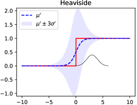
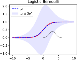
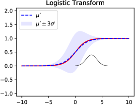
Figure 2: Propagation for different non-linearities. Heaviside function: $Y=\mathchoice{\hbox to0.0pt{$\displaystyle{[}$\hss}}{\hbox to0.0pt{$\textstyle{[}$\hss}}{\hbox to0.0pt{$\scriptstyle{[}$\hss}}{\hbox to0.0pt{$\scriptscriptstyle{[}$\hss}}\hskip 1.3pt[X{\geq}0]\hskip 1.36pt\mathchoice{\hbox to0.0pt{\hss$\displaystyle{]}$}}{\hbox to0.0pt{\hss$\textstyle{]}$}}{\hbox to0.0pt{\hss$\scriptstyle{]}$}}{\hbox to0.0pt{\hss$\scriptscriptstyle{]}$}}$, Bernoulli-logistic: $Y$ is a Bernoulli r.v. with $p(Y{=}1\,|\,X)=\mathcal{S}(X)$ and logistic-transform: $Y=\mathcal{S}(X)$. Red: activation function. Black: an exemplary input distribution with mean $\mu=3$, variance $\sigma^{2}=1$ shown with support $\mu\pm 3\sigma$. Dashed blue: the approximate mean $\mu^{\prime}$ of the output versus the input mean $\mu$. The variance of the output is shown as blue shaded area $\mu^{\prime}\pm 3\sigma^{\prime}$.

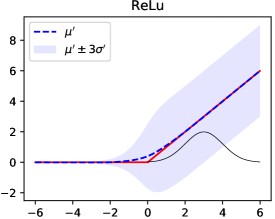
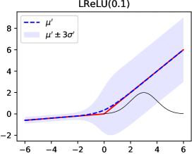
Figure 3: Propagation in ReLU: $\max(0,X)$ and leaky ReLU: $\max(X,\alpha X)$ with $\alpha=0.1$.

Other Layers

The same principle can be applied to propagation in other layers. For example, statistics of the product $X_{1}X_{2}$ of independent r.v.’s express as

$$\mu^{\prime}=\mu_{1}\mu_{2};\ \ \ \ \ \ \ \sigma^{\prime 2}=\sigma_{1}^{2}\sigma_{2}^{2}+\sigma_{1}^{2}\mu_{2}^{2}+\mu_{1}^{2}\sigma_{2}^{2}.$$ (8)

This is used, e.g., in the propagation through dropout, which can be viewed as multiplicative Bernoulli noise. We derive an approximation for the maximum of two independent random variables $\max(X_{1},X_{2})$, which allows to model maxOut and max pooling (in the latter we need to compose the maximum of many variables hierarchically, assuming conditional independence). Closely related to the maximum and crucial in classification problems, is the softmax layer. We derive several approximations to it, of varying complexity and accuracy.

3.3 Sigmoid Belief Networks

A Simple Approximation

Sigmoid belief networks [24] are an important special case in which standard neural networks can be viewed as an approximation to the inference.

Let $X$ denote a layer of units and $Y$ denote a single hidden unit with $p(Y{=}1\,|\,X)=\mathcal{S}(w^{\mathsf{T}}X)$ . The required propagation (4) expresses as $q(Y{=}1)=\mathbb{E}_{q(X)}\mathcal{S}(w^{\mathsf{T}}X)$. The first order Taylor series expansion for the mean results in the approximation [5, 7]:

$$\mathbb{E}_{q(X)}\mathcal{S}(w^{\mathsf{T}}X)\approx\mathcal{S}(w^{\mathsf{T}}\mathbb{E}_{q(X)}X),$$ (AP1)

i.e., the expectation is substituted under the function. Using the mean parameters $\mu^{X}_{i}=q(X_{i}{=}1)$, the approximation can be written as $\mu^{Y}=\mathcal{S}(w^{\mathsf{T}}\mu^{X})$ and we recover the standard forward propagation rule in a sigmoid NN. The following example shows that this approximation may be significantly under- or overestimating.

Example 1 (Logical AND).

Consider a unit that has to perform logical reasoning with uncertain inputs such as: if we see a car wheel with probability 50% and a car roof with probability 30%, what is the probability that the two parts are present simultaneously? Let the two binary inputs $X_{1},X_{2}$ have probabilities $p(X_{1}{=}1)$ and $p(X_{2}{=}1)$, respectively. We want to approximate the true expectation of $X_{1}\wedge X_{2}$ that both inputs are active. We evaluate the logistic model $p(Y{=}1\,|\,X)=\mathcal{S}(a(X_{1}+X_{2})+b)$. The parameters $a,b$ are chosen as follows: for the input $(1,1)$ we require probability $P(Y{=}1\,|\,X)$ to be at least $1-\varepsilon$ and for inputs $(1,0)$ or $(0,1)$ it must be at most $\varepsilon$. For $\varepsilon=0.05$ this gives $a=5.89$ and $b=-1.5$, see § 0.B.3. We then compare the exact expectation of the logistic model $\mathbb{E}[Y]=\mathbb{E}_{X}[p(Y{=}1\,|\,X)]$ and the approximation by Eq. AP1. Results in Table 1 show that the expectation of the logistic model fits $\mathbb{E}[X_{1}\wedge X_{2}]$ accurately, while the approximation AP1 is severely underestimating and does not distinguish the cases $(0,1)$ and $(0.5,0.5)$.

$p(X_{1}{=}1)$	$p(X_{2}{=}1)$	$\mathbb{E}[X_{1}{\wedge}X_{2}]$	$\mathbb{E}[Y]$	AP1
0	0	0	0.00015	0.00015
0	1	0	0.05	0.05
1	1	1	0.95	0.95
0.25	0.25	0.0625	0.077	0.0027
0.5	0.5	0.25	0.26	0.05
0.75	0.75	0.56	0.55	0.5

Table 1: Logic AND gate in the expectation, Logistic model and standard NN.

This example shows a conceptual flaw in viewing the sigmoid NN as a hierarchy of part detectors since the probabilities estimated by the units in a hidden layer are not taken into account correctly in the next layer. Approximating the OR gate with a standard NN runs into a similar problem of overestimating the probability. A more accurate approximation can be extremely useful in modeling logic gates and robust statistics of uncertain inputs.

Improved Approximation: Latent Variable Model

We now derive a better approximation for the expectation of the logistic Bernoulli unit making some assumptions about the input. The approximation is essentially similar to [18, eq. 8], but we explain the latent variable view, which leads to somewhat different constants an will be important for treating the softmax.

The difficulty in computing $\mathbb{E}_{q(X)}[\mathcal{S}(w^{\mathsf{T}}X)]$ stems from the fact that $X_{i}$ are binary and therefore the activation $U=w^{\mathsf{T}}X$ has a discrete distribution with mass in combinatorially many points. Noting that $\mathcal{S}$ is itself the cdf of a logistic distribution, we make the following observation (known as “latent variable model” in logistic regression, see also Bernoulli-logistic unit [36, p.4])

Observation 1.

Let $Z$ be a r.v. with cdf $\mathcal{S}$, independent from $X$. Then $\mathbb{E}[\mathcal{S}(w^{\mathsf{T}}X)]=\Pr\{w^{\mathsf{T}}X-Z\geq 0\}$.

Proof.

Since $\mathcal{S}(z)=\Pr\{Z\,{\leq}\,z\}$ we have $\mathbb{E}S(w^{\mathsf{T}}X)=\mathbb{E}_{X}\Pr\{Z\leq w^{\mathsf{T}}X\,|\,X\}=\Pr\{w^{\mathsf{T}}X-Z\geq 0\}$. ∎

The density of the difference $w^{\mathsf{T}}X-Z$ is given by the convolution of the discrete density of $w^{\mathsf{T}}X$ with a smooth bell-shaped logistic density of $Z$. This efficiently smooths the discrete density of $U$ and the distribution of $w^{\mathsf{T}}X-Z$ tends to normality when weights $w$ are random or bounded and the dimension increases. It allows to use the following approximation:

Proposition 1.

Assuming that $w^{\mathsf{T}}X-Z$ has normal distribution, we can approximate

$$\mathbb{E}_{X}\mathcal{S}(w^{\mathsf{T}}X)\approx\Phi(\mu/(\sigma^{2}+\sigma^{2}_{\mathcal{S}})^{\frac{1}{2}}),$$ (AP2a)

where $\Phi$ is the cdf of standard normal distribution, $\mu=\mathbb{E}(w^{\mathsf{T}}X)$, $\sigma^{2}=\operatorname{Var}(w^{\mathsf{T}}X)$ and $\sigma^{2}_{\mathcal{S}}=\pi^{2}/3$ is the variance of the standard logistic distribution.

It is obtained as follows. We compute the mean and variance of $V=w^{\mathsf{T}}X-Z$ as $\mathbb{E}[V]=\mathbb{E}[w^{\mathsf{T}}X]-\mathbb{E}[Z]$ and $\operatorname{Var}[V]=\operatorname{Var}[w^{\mathsf{T}}X]+\operatorname{Var}[Z]$. The probability $\Pr\{V>0\}$ is given by $1-F_{V}(0)$, where $F_{V}$ is the cdf of $V$, which is assumed normal. Expressing $1-F_{V}(0)$ through the cdf of the standard normal distribution $\Phi$ we obtain Eq. AP2a. The following variant is even simpler to compute.

Proposition 2.

Assuming that $w^{\mathsf{T}}X-Z$ has logistic distribution, we can approximate

$$\mathbb{E}_{X}\mathcal{S}(w^{\mathsf{T}}X)\approx\mathcal{S}(\mu/s),$$ (AP2b)

where $s=(\sigma^{2}/\sigma^{2}_{\mathcal{S}}+1)^{\frac{1}{2}}$, $\mu=\mathbb{E}[w^{\mathsf{T}}X]$, $\sigma^{2}=\operatorname{Var}(w^{\mathsf{T}}X)$.

The scale parameter $s$ is chosen so that the variance of the standard logistic distribution $s^{2}\sigma^{2}_{\mathcal{S}}$ matches that of $w^{\mathsf{T}}X-Z$. It is remarkable that (AP2b) differs from (AP1) only by the scale of the activation. However this scaling is dynamic: it depends on the network parameters and the input.

Illustrations and comparison of accuracy of these approximations are given in § 0.C.3. The variance of the logistic Bernoulli unit is defined by (4). The logistic transform $Y=\mathcal{S}(X)$ happens to have exactly the same mean, because the mean of the Bernoulli distribution is its probability of drawing $1$. However, the variance of $Y=\mathcal{S}(X)$, illustrated in Fig. 2, is different and poses a separate challenge detailed in § 0.C.4.

3.4 General Latent Variable Models

Latent Variable Models, as in § 3.3, on one hand help us to compute expectations of some functions and on the other hand form a rich source of stochastic models. This allows to give a universal treatment to sigmoid belief networks, neural networks with uncertain inputs, networks with injected noise and possible combinations thereof.

We start from the latent variable representation of a sigmoid belief network layer $p(Y_{j}{=}1\,|\,X)=\mathcal{S}(w^{\mathsf{T}}X)$, which reads as $Y_{j}=\mathchoice{\hbox to0.0pt{$\displaystyle{[}$\hss}}{\hbox to0.0pt{$\textstyle{[}$\hss}}{\hbox to0.0pt{$\scriptstyle{[}$\hss}}{\hbox to0.0pt{$\scriptscriptstyle{[}$\hss}}\hskip 1.3pt[w^{\mathsf{T}}X+Z\geq 0]\hskip 1.36pt\mathchoice{\hbox to0.0pt{\hss$\displaystyle{]}$}}{\hbox to0.0pt{\hss$\textstyle{]}$}}{\hbox to0.0pt{\hss$\scriptstyle{]}$}}{\hbox to0.0pt{\hss$\scriptscriptstyle{]}$}}$, $Z\sim\mathcal{S}$. It is straightforward to generalize Observation 1 to other activations that have the form of a cdf, by considering the respective noise. More interestingly, different functions may be used in place of the thresholding function. Consider the following latent variable (injected noise) model:

$$X^{k}=f(W^{k}X^{k-1}-Z^{k}),$$ (9)

where $f\colon\mathbb{R}\to\mathbb{R}$ is applied component-wise and $Z^{k}_{i}$ is an independent real-valued r.v. with a known distribution (such as the standard normal distribution).

From representation (9) we can reconstruct back the conditional cdf of the belief network $F_{X^{k}\,|\,X^{k-1}}(u)=\mathbb{E}_{Z^{k}}[W^{k}f(X^{k-1}-Z^{k})\leq u]$ and the respective conditional density. Examples for the stochastic binary neuron $Y=\mathchoice{\hbox to0.0pt{$\displaystyle{[}$\hss}}{\hbox to0.0pt{$\textstyle{[}$\hss}}{\hbox to0.0pt{$\scriptstyle{[}$\hss}}{\hbox to0.0pt{$\scriptscriptstyle{[}$\hss}}\hskip 1.3pt[w^{\mathsf{T}}X-Z]\hskip 1.36pt\mathchoice{\hbox to0.0pt{\hss$\displaystyle{]}$}}{\hbox to0.0pt{\hss$\textstyle{]}$}}{\hbox to0.0pt{\hss$\scriptstyle{]}$}}{\hbox to0.0pt{\hss$\scriptscriptstyle{]}$}}$ considered in [36] with general noise and the stochastic rectifier $Y=\max(w^{\mathsf{T}}X-Z,0)$ considered in [3] are given in § 0.B.1. The conditional density may however be complicated and its explicit form is in fact not needed for our approximate inference. The moments of $f(W^{k}X^{k-1}-Z^{k})$ can be computed directly, provided that the components of $W^{k}X^{k-1}-Z^{k}$ are assumed to have an approximate distribution density $q$ such that the integral $\int_{u}q(u)f(u)\>du$ can be computed in closed form. For many non-linearities used in NNs, we can do so with either normal or logistic distribution, similarly to approximations Eq. AP2a, Eq. AP2b.

3.5 Softmax

Softmax is the multinomial logistic model: $p(Y{=}y\,|\,X)=\exp(X_{y})/\sum_{i}\exp(X_{i})$. Assuming there are $n$ classes, the posterior approximate distribution $q(Y)$ is specified by $n$ numbers. The expectation over $X$ in this case is more difficult since it is $n$-dimensional. Fortunately, it is expressible in the latent variable model (cf. Observation 1) using multidimensional noise:

$$\textstyle\mathbb{E}[p(Y{=}y\,|\,X)]=\Pr\{U-Z\geq 0\},$$ (10)

where $U$ is a r.v. in $\mathbb{R}^{n-1}$ with components $U_{k}=X_{y}-X_{k}$ for $k\neq y$ and $Z$ has an $n{-}1$-variate logistic distribution [20]. We make a simplification by using an i.i.d. logistic model for $Z_{k}$ in (10). We can then build approximations by assuming that $U-Z$ is multivariate normal or multivariate logistic and evaluate the respective cdf instead of $\Pr\{U-Z\geq 0\}$. The logistic approximation gives the expression

$$q(y)\approx\Big{(}1+\sum_{k\neq y}\exp\Big{\{}\frac{\mu_{k}-\mu_{y}}{\textstyle\sqrt{(\smash[b]{\sigma^{2}_{k}+\sigma^{2}_{y}})/\smash[b]{\sigma^{2}_{\mathcal{S}}+1}}}\Big{\}}\Big{)}^{-1}.$$ (11)

A drastically simplified approximation, which we use in the end-to-end training, reduces to the softmax of $\mu_{k}/\sqrt{\sigma_{k}^{2}/\sigma_{S}^{2}+1}$. See the derivations in § 0.C.7. When the input variances are zero, both approximations recover the standard softmax function.

3.6 End-to-end Training

Let $q(X^{l}\,|\,x^{0};\theta)$ denote the output probabilities of our model. We consider standard learning optimization objectives. For classification, we maximize the conditional likelihood of the training data, i.e., we minimize

$$L=\mathbb{E}_{(x^{0},x^{l*})\sim{\rm data}}\big{[}{-}\log q(X^{l}=x^{l*}\,|\,x^{0};\theta)\big{]}.$$ (12)

Continuous Differentiability

The derivative w.r.t. parameters is obtained by back-propagation expanding derivatives in both mean and variance dependencies. We observe that all propagation equations based on computing expectations w.r.t. Gaussian or logistic distribution are continuously differentiable assuming non-zero variance. In order to allow for learning with hard non-linearities, such as the Heaviside function, it is sufficient to assume that each input instance has some uncertainty or that the first layer is stochastic. Typically used heuristics such as replacing the step function with identity in the backward pass can be avoided.

Gradients

In the approximations for different non-linear transforms such as Eq. AP2b (full list in § 0.C), the mean is always divided by the standard deviation whenever it occurs in saturating functions such as $\Phi,\phi,\mathcal{S}$. When hidden units are uncertain, the variance is larger and all non-linearities automatically become smoother. The automatic scaling by uncertainty allows the gradient to be propagated deeper through the network. The space of parameters where $\mu/\sigma$ is small, as opposed to where $\mu$ is small in standard networks, and the gradients do not vanish is different and may be larger.

4 Experiments

Implementation

Our implementation (in pytorch) will be made available upon acceptance. Important for our experiments, the implementation is modular: with each of the standard layers we can do 3 kinds of propagation: AP1: standard propagation in deterministic layers and taking the mean in stochastic layers (e.g., in dropout we need to multiply by the Bernoulli probability), AP2: proposed propagation rules with variances and sample: by drawing samples of any encountered stochasticity (such as sampling from Bernoulli distribution in dropout). The last method is also essential for computing Monte Carlo (MC) estimates of the statistics we are trying to approximate. When the training method is sample, the test method is assumed to be AP1, which matches the standard practice of dropout training. Details of the implementation and models are given in § 0.D.

CA C A C A F Softmax LReLU, Noisy input $\mathcal{N}(0,10^{-4})$ $\varepsilon_{\mu_{1}}$ 0.02 0.04 0.04 0.06 0.05 0.08 KL 1.4e-6 $\varepsilon_{\mu_{2}}$ 0.02 0.02 0.02 0.03 0.02 0.03 KL 4.5e-7 $\varepsilon_{\sigma_{2}}$ 1.01 0.88 0.87 0.64 0.63 0.63 KL’ 3.8e-7 LReLU, Noisy input $\mathcal{N}(0,0.01)$ $\varepsilon_{\mu_{1}}$ 0.14 0.29 0.24 0.60 0.45 0.67 KL 0.03 $\varepsilon_{\mu_{2}}$ 0.02 0.03 0.03 0.05 0.05 0.08 KL 0.003 $\varepsilon_{\sigma_{2}}$ 1.07 0.91 0.91 0.68 0.58 0.69 KL’ 0.002 LReLU, Noisy input $\mathcal{N}(0,0.1)$ $\varepsilon_{\mu_{1}}$ 0.31 0.74 0.51 1.47 1.11 1.60 KL 5.09 $\varepsilon_{\mu_{2}}$ 0.03 0.04 0.05 0.06 0.07 0.10 KL 0.07 $\varepsilon_{\sigma_{2}}$ 1.12 0.99 1.09 0.75 0.65 0.79 KL’ 0.03 CA C A C A F Softmax LReLU, Dropout (0.2) $\varepsilon_{\mu_{1}}$ 0.01 0.02 0.04 0.17 0.06 0.10 KL 0.02 $\varepsilon_{\mu_{2}}$ 0.01 0.02 0.01 0.03 0.02 0.03 KL 9.5e-3 $\varepsilon_{\sigma_{2}}$ 1.00 1.00 1.01 0.95 0.98 0.95 KL’ 2.9e-3 Logistic Bernoulli $\varepsilon_{\mu_{1}}$ 0.02 0.02 0.13 0.20 0.20 0.17 KL 6.0 $\varepsilon_{\mu_{2}}$ 0.02 0.02 0.03 0.04 0.08 0.07 KL 0.06 $\varepsilon_{\sigma_{2}}$ 1.09 1.00 1.00 0.69 0.95 0.93 KL’ 1.2e-2 Logistic Transform, Noisy input $\mathcal{N}(0,0.1)$ $\varepsilon_{\mu_{1}}$ 0.06 0.17 0.17 0.40 0.38 0.53 KL 0.01 $\varepsilon_{\mu_{2}}$ 0.03 0.05 0.05 0.12 0.12 0.17 KL 2.6e-3 $\varepsilon_{\sigma_{2}}$ 1.00 1.10 1.09 0.72 0.72 0.90 KL’ 1.4e-2

Table 2: Accuracy of approximation for LeNet/MNIST Model per layer. Columns: C - conv layer, A - activation, F - fully connected. In the case of dropout, it is included in the activation. Rows: $\varepsilon_{\mu_{1}}$ - error of approximation of the mean by the standard method (AP1), $\varepsilon_{\mu_{2}},\varepsilon_{\sigma_{2}}$ errors of approximation by the proposed method (AP2). Errors in $\mu$ are relative to average MC $\sigma^{*}$, errors in $\sigma$ show the multiplicative factor of $\sigma^{*}$ (see text). In the final layer we show KL divergence of the class posterior from MC class posterior. For AP2 two versions are evaluated: using simplified approximation of softmax and full approximation of softmax (KL’).

Approximation Accuracy

Tables 2 and 3 report approximation accuracy per layer in LeNet and CIFAR networks for different use cases. All models with LReLU use $\alpha=0.01$. We have computed MC statistics $\mu^{*},\sigma^{*}$ per unit in each layer. The error measure of the means $\varepsilon_{\mu}$ is the average $|\mu-\mu^{*}|$ relative to the average $\sigma^{*}$. The averages are taken over all units in the layer and over input images. The error of the standard deviation $\varepsilon_{\sigma}$ is the geometric mean of $\sigma/\sigma^{*}$, representing the error as a factor from the true value (e.g., $1.0$ is exact, $0.9$ is under-estimating and $1.1$ is over-estimating). MC estimates are using $10^{3}$ samples, which was sufficient to compute 2 significant digits as reported.

The following can be observed from the results in Tables 2 and 3. The propagation of the input uncertainty works reasonably well for LeNet network (4 pairs of linear and activation layers) but degrades with more layers as seen for CIFAR network in Table 3. This is to be expected since the errors of the approximation accumulate. The main contribution to the loss of accuracy comes from the poor approximation of the variance in the convolutional layers, where we ignored dependencies. This is clearly seen in the case of small input noise where the accuracy in $\sigma$ drops significantly after the convolutional layers. It means that the inputs are positively correlated on average so that ignoring this correlation underestimates the variance.

Differently from propagating input uncertainty through deep networks, in the case of dropout and Bernoulli models the uncertainty created by a layer appears to dominate the uncertainty propagated from the preceding layers and thus the estimation does not degrade.

	C	A	C	A	C	A	C	A	C	A	C	A	C	A	C	A	C	P	Softmax
LReLU, Noisy input $\mathcal{N}(0,0.01)$
$\varepsilon_{\mu_{1}}$	0.02	0.24	0.39	0.37	0.76	0.63	1.13	0.85	1.59	1.10	1.93	1.32	2.65	1.86	2.76	1.93	1.99	2.59	KL	4.42
$\varepsilon_{\mu_{2}}$	0.02	0.02	0.03	0.19	0.49	0.36	0.55	0.42	0.73	0.55	0.96	0.68	1.26	0.97	1.27	1.01	1.14	1.43	KL	1.71
$\varepsilon_{\sigma_{2}}$	1.00	1.11	0.59	0.40	0.37	0.28	0.35	0.19	0.26	0.10	0.17	0.05	0.11	0.05	0.08	0.04	0.07	0.07	KL’	1.71
LReLU, Dropout (0.2)
$\varepsilon_{\mu_{1}}$	-	0.01	0.02	0.04	0.12	0.07	0.13	0.09	0.17	0.11	0.21	0.14	0.26	0.14	0.27	0.16	0.23	0.32	KL	0.05
$\varepsilon_{\mu_{2}}$	-	0.01	0.02	0.01	0.02	0.02	0.03	0.02	0.04	0.03	0.05	0.04	0.08	0.05	0.08	0.07	0.10	0.15	KL	0.02
$\varepsilon_{\sigma_{2}}$	-	1.00	1.00	1.02	0.93	0.95	0.90	0.92	0.81	0.79	0.73	0.69	0.71	0.69	0.71	0.65	0.56	0.69	KL’	0.02
Logistic Bernoulli
$\varepsilon_{\mu_{1}}$	-	0.02	0.02	0.04	0.12	0.10	0.18	0.15	0.29	0.21	0.37	0.25	0.48	0.31	0.44	0.33	0.27	0.47	KL	3.46
$\varepsilon_{\mu_{2}}$	-	0.02	0.02	0.03	0.04	0.04	0.05	0.06	0.12	0.10	0.20	0.14	0.30	0.19	0.28	0.19	0.14	0.25	KL	0.21
$\varepsilon_{\sigma_{2}}$	-	1.12	1.00	1.02	0.92	0.99	0.78	0.97	0.59	0.95	0.56	0.94	0.61	0.94	0.73	0.96	0.74	0.99	KL’	0.1
Logistic Transform, Noisy input $\mathcal{N}(0,0.01)$
$\varepsilon_{\mu_{1}}$	0.02	0.17	0.17	0.28	0.49	0.53	0.98	0.96	1.47	1.39	1.62	1.52	2.13	2.06	2.36	2.31	1.86	2.55	KL	3.46
$\varepsilon_{\mu_{2}}$	0.02	0.03	0.03	0.16	0.40	0.43	0.82	0.81	1.26	1.21	1.39	1.32	1.88	1.84	2.05	2.03	1.60	2.20	KL	2.68
$\varepsilon_{\sigma_{2}}$	1.00	1.01	0.40	0.41	0.28	0.29	0.23	0.23	0.12	0.11	0.05	0.05	0.02	0.02	0.01	0.01	0.01	0.01	KL’	2.68

Table 3: Accuracy of approximation for CIFAR-10 Model. The notation is the same as in Table 2, the row “P” in the head of the networks is the average pooling layer.

LReLU C A C A C A F Init=None $\mu$ 0.10 0.27 0.23 0.22 0.39 0.33 0.41 $\sigma$ 0.89 1.32 0.85 1.01 0.92 1.03 0.93 Init=BN $\mu$ 0.10 0.49 0.13 0.36 0.29 0.52 0.49 $\sigma$ 0.89 1.20 1.04 1.22 1.28 1.47 1.49 Init=AP2 $\mu$ 0.10 0.20 0.26 0.25 0.38 0.37 0.38 $\sigma$ 0.89 1.23 0.92 1.17 1.08 1.37 1.21

Logistic Transform C A C A C A F Init=None $\mu$ 0.10 0.09 0.24 0.24 0.36 0.36 0.27 $\sigma$ 0.89 0.91 0.76 0.76 0.76 0.77 0.75 Init=BN $\mu$ 0.10 0.04 0.20 0.19 0.34 0.34 0.25 $\sigma$ 0.93 1.06 1.02 1.10 1.15 1.16 1.16 Init=AP2 $\mu$ 0.10 0.04 0.17 0.15 0.37 0.37 0.28 $\sigma$ 0.89 1.15 1.02 1.13 1.16 1.22 1.21

Table 4: Accuracy of dataset statistics for LeNet/MNIST, estimated by AP2 model with a single-pixel input $(\mu_{0},\sigma_{0}^{2})$. The notation is the same as in Table 2.

Dataset Statistics and Analytic Normalization

Table 4 shows the accuracy of estimating neuron statistics over the dataset using the proposed technique. In convolutional networks, the task is to estimate the mean and variance $\mu^{*},\sigma^{*}$ per channel in each layer, i.e., the statistics are over the input dataset and the spatial dimensions. With our method, the estimates are computed by propagating through the network the statistics of the input dataset $\mu^{*}_{0},\sigma^{*}_{0}$ (that obviously do not depend on the network). The propagation works directly with spatial averages, the batch dimension and the spatial dimensions are not used and the only relevant dimension is channels (see details of this efficient implementation in [32]). The reported errors in estimating the statistics are averaged over the channels. We study these errors for three cases: randomly initialized networks, networks re-initialized with batch normalization (BN) [11] as described e.g. in [30] and our analytic normalization [32]. The re-initialization consists of recurrently going through the layers, applying the normalization and estimating the statistics of the next layer. It is clearly seen that the accuracy of the analytic normalization is completely sufficient for the purpose of network initialization and normalization [32] (i.e. the true variance is close to one and the deviation from the true mean is less than the true standard deviation). This normalization is computationally cheap, continuously differentiable and is applicable to training of standard networks as well as variance-propagating networks. In comparison to BN, it however lacks additional generalization properties [32].

Analytic Dropout

In this experiment we demonstrate the utility of using our approximation during training. Fig. 4 shows a comparison of plain training, dropout [33], which samples multiplicative Bernoulli noise during training, and analytic dropout, in which our propagation is used. The dropout layers are applied after every activation and there is no input dropout. All methods start from the same BN-initialized point and use the same learning rate and schedule ($0.001\cdot 0.96^{k}$ in epoch $k$) and the same optimizer (Adam [13]). We intentionally do not use batch normalization during training, since it has a regularization effect of its own [11] that needs to be studied separately. With the analytic propagation we show two results: initialized the same way as the baseline and using [32]. This comparison is limited but it shows that AP2 propagation significantly improves validation error in a deep network while not slowing the training down, which qualitatively agrees with the findings of [35] for smaller networks.

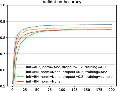
Figure 4: CIFAR-10: Comparison of plain training, dropout and analytic dropout for drop probabilities 0.2 and 0.3. For the analytic dropout (training=AP2) we tested two variants: with the same initialization as the baseline and with AP2 initialization and normalization. The plots show validation accuracies during training epochs (running average). Notice that dropout (green) fails to improve the validation accuracy compared to standard training (red) for higher drop probability within the training schedule. The proposed analytic dropout clearly improves the validation accuracy without a noticeable slow down.

Stability

We made a conjecture that propagating uncertainty may improve stability of the predictions under noise or adversarial attacks. The idea can be demonstrated on a simple NN with one hidden layer of 100 units. This simple model trained on the MNIST dataset reveals quite surprising results. We compared training of a standard NN with sigmoid activations and a model with Bernoulli-logistic activations trained using AP2, assuming input noise with variance $0.1$. The results in Fig. 5 show that the latter model, while achieving the same test accuracy, is significantly more stable to Gaussian noise. The same dependance is observed for gradient sign attack [9] shown in Fig. 0.D.1. The shown stability results do not immediately scale to deep networks. We see two reasons for this. First, the approximation quality of propagating input uncertainty degrades with depth as we have seen above. Second, the stability depends on both the propagation method and the choice of parameters. While propagating variance can deliver a more stable classifier, the choice of parameters is still crucial. In particular, parameters may exist such that the network posterior is always deterministic regardless of the input uncertainty. In this case, propagating the variance is useless. These issues need to be addressed in the future work.

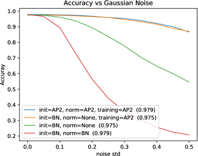
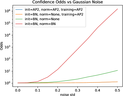
Figure 5: Stability evaluation of MLP/MNIST model under Gaussian noise. All networks have similar test accuracy in the noise-free scenario (numbers in brackets). Bernoulli model with analytic propagation shows a better stability w.r.t. random perturbations of the input. Batch normalization achieves a lower training loss than the standard NN which leads to a significant drop in the stability. When the network trained with BN makes errors under noise it does so with a very high confidence odds – the ratio of the predicted class probability over the true one: $\max_{y}q(y)/q(y^{*})$.

5 Conclusion

We have described an inference method which lies between feed-forward neural networks and iterative inference methods such as variational methods or belief propagation in Bayesian networks. We have build a framework of variance-propagating layers, extending constructive elements of standard NNs, in which a range of models can be considered with deterministic and stochastic units and used in end-to-end learning. The feed-forward structure is one one hand restrictive, because we can only perform inference in one direction. On the other hand, it allows dealing with uncertainties in NNs and opens a number of possibilities with practical benefits. The quality of the approximation of posterior probabilities can be measured. The accuracy is sufficient for several use cases such as sigmoid belief nets, dropout training and normalization techniques. It may be insufficient for propagating input uncertainties through a deep network, but we believe that a calibration will be possible. Further applications may include generative and semi-supervised learning (VAE) and Bayesian model estimation.

Appendix toc

Appendix 0.A Used Facts on Approximate Marginalization

Lemma 0.A.1.

Let $X$ be a r.v. with components $X_{i}$ and pdf $p(X)$. The closest factorized approximation $q(X)=\prod_{i}q(X_{i})$ to $p(X)$ in terms of forward KL divergence is given by the marginals $p(x_{i})=\sum_{(x_{j}\,|\,j\neq i)}p(x)$.

Proof.

Minimizing

$$KL(p(X)\|q(X))=\mathbb{E}_{p(X)}\log\frac{p(X)}{q(X)},$$ (13)

in $q$ is equivalent to maximizing

$$\mathbb{E}_{p(X)}\log{q(X)}.$$ (14)

Assuming $q(X)=\prod_{i}q(X_{i})$, the negative cross-entropy above expresses as

$$\sum_{x}p(x)\sum_{i}\log q(x_{i})=\sum_{i}\sum_{x_{i}}p(x_{i})\log q(x_{i}),$$ (15)

which is maximum when $q(x_{i})=p(x_{i})$. ∎

Lemma 0.A.2.

Let $X$ be a continuous r.v. The closest approximation to $p(X)$ by a Gaussian $q(x)=\frac{1}{\sqrt{2\pi}\sigma}\exp(-\frac{(x-\mu)^{2}}{2\sigma^{2}})$ in forward KL divergence is given by moment matching: $\mu=\mathbb{E}[X]$, $\sigma^{2}=\mathbb{E}[X_{2}-\mu]$.

Proof.

This is essentially the same as in maximum likelihood estimate of normal distribution. Differentiating (14) and solving for the critical point we get for the mean

$$0=E_{p(X)}\frac{\partial}{\partial\mu}\log q(X)=\mathbb{E}_{p(X)}\frac{(X-\mu)}{\sigma^{2}},$$ (16)

from which $\mu=\mathbb{E}_{p(X)}[X]$. And for the variance:

$$0=E_{p(X)}\frac{\partial}{\partial\sigma}\log q(X)=\mathbb{E}_{p(X)}\Big{(}-\frac{1}{\sigma}+\frac{(X-\mu)^{2}}{\sigma^{3}}\Big{)},$$

from which $\sigma^{2}=\mathbb{E}_{p(X)}[(X-\mu)^{2}]$. ∎

Appendix 0.B Auxiliary Results

0.B.1 From Latent Variable Model to Belief Network

Lemma 0.B.1 (Stochastic binary neuron).

Let $Y=\mathchoice{\hbox to0.0pt{$\displaystyle{[}$\hss}}{\hbox to0.0pt{$\textstyle{[}$\hss}}{\hbox to0.0pt{$\scriptstyle{[}$\hss}}{\hbox to0.0pt{$\scriptscriptstyle{[}$\hss}}\hskip 1.3pt[X-Z\geq 0]\hskip 1.36pt\mathchoice{\hbox to0.0pt{\hss$\displaystyle{]}$}}{\hbox to0.0pt{\hss$\textstyle{]}$}}{\hbox to0.0pt{\hss$\scriptstyle{]}$}}{\hbox to0.0pt{\hss$\scriptscriptstyle{]}$}}$, where $Z$ is independent r.v. with cdf $F_{Z}$. Then $\Pr(Y{=}1\,|\,X)=F_{Z}(X)$.

Proof.

We have

$$\Pr(Y{=}1\,|\,X)=\mathbb{E}\big{[}\mathchoice{\hbox to0.0pt{$\displaystyle{[}$\hss}}{\hbox to0.0pt{$\textstyle{[}$\hss}}{\hbox to0.0pt{$\scriptstyle{[}$\hss}}{\hbox to0.0pt{$\scriptscriptstyle{[}$\hss}}\hskip 1.3pt[X-Z\geq 0]\hskip 1.36pt\mathchoice{\hbox to0.0pt{\hss$\displaystyle{]}$}}{\hbox to0.0pt{\hss$\textstyle{]}$}}{\hbox to0.0pt{\hss$\scriptstyle{]}$}}{\hbox to0.0pt{\hss$\scriptscriptstyle{]}$}}\bigm{|}X\big{]}=\mathbb{E}\big{[}\mathchoice{\hbox to0.0pt{$\displaystyle{[}$\hss}}{\hbox to0.0pt{$\textstyle{[}$\hss}}{\hbox to0.0pt{$\scriptstyle{[}$\hss}}{\hbox to0.0pt{$\scriptscriptstyle{[}$\hss}}\hskip 1.3pt[Z\leq X]\hskip 1.36pt\mathchoice{\hbox to0.0pt{\hss$\displaystyle{]}$}}{\hbox to0.0pt{\hss$\textstyle{]}$}}{\hbox to0.0pt{\hss$\scriptstyle{]}$}}{\hbox to0.0pt{\hss$\scriptscriptstyle{]}$}}\bigm{|}X\big{]}=F_{Z}(X).$$ (17)

∎

Thus, a stochastic binary neuron with logistic noise is equivalent to a Bernoulli-logistic unit [36, p.4] (this is a well-known interpretation in logistic regression) and such networks are equivalent to logistic belief nets [24].

Lemma 0.B.2 (Stochastic Rectifier).

Let $Y=\max(0,X-Z)$, where $Z$ is an independent r.v. with cdf $F_{Z}$ and pdf $p_{Z}$. Then $p(Y{=}y\,|\,X)=(1-F_{Z}(X-y))\delta_{0}(y)+p_{Z}(X-y)\mathchoice{\hbox to0.0pt{$\displaystyle{[}$\hss}}{\hbox to0.0pt{$\textstyle{[}$\hss}}{\hbox to0.0pt{$\scriptstyle{[}$\hss}}{\hbox to0.0pt{$\scriptscriptstyle{[}$\hss}}\hskip 1.3pt[y{>}0]\hskip 1.36pt\mathchoice{\hbox to0.0pt{\hss$\displaystyle{]}$}}{\hbox to0.0pt{\hss$\textstyle{]}$}}{\hbox to0.0pt{\hss$\scriptstyle{]}$}}{\hbox to0.0pt{\hss$\scriptscriptstyle{]}$}}$, where $\delta$ is the Dirac distribution.

Proof.

Let us begin with deriving the conditional cdf. of $Y$. We have

$$\Pr\{Y\,{\leq}\,y\,|\,X\} =\mathbb{E}\big{[}\mathchoice{\hbox to0.0pt{$\displaystyle{[}$\hss}}{\hbox to0.0pt{$\textstyle{[}$\hss}}{\hbox to0.0pt{$\scriptstyle{[}$\hss}}{\hbox to0.0pt{$\scriptscriptstyle{[}$\hss}}\hskip 1.3pt[\max(0,X-Z)\leq y]\hskip 1.36pt\mathchoice{\hbox to0.0pt{\hss$\displaystyle{]}$}}{\hbox to0.0pt{\hss$\textstyle{]}$}}{\hbox to0.0pt{\hss$\scriptstyle{]}$}}{\hbox to0.0pt{\hss$\scriptscriptstyle{]}$}}\bigm{|}X\big{]}$$ (18)

$$=\mathbb{E}\big{[}\mathchoice{\hbox to0.0pt{$\displaystyle{[}$\hss}}{\hbox to0.0pt{$\textstyle{[}$\hss}}{\hbox to0.0pt{$\scriptstyle{[}$\hss}}{\hbox to0.0pt{$\scriptscriptstyle{[}$\hss}}\hskip 1.3pt[\min(X,Z)\geq X-y]\hskip 1.36pt\mathchoice{\hbox to0.0pt{\hss$\displaystyle{]}$}}{\hbox to0.0pt{\hss$\textstyle{]}$}}{\hbox to0.0pt{\hss$\scriptstyle{]}$}}{\hbox to0.0pt{\hss$\scriptscriptstyle{]}$}}\bigm{|}X\big{]}$$ (19)

The indicator function is obviously zero if $y<0$. If, on the other hand, $y\geq 0$ then the indicator function is nonzero only if $Z\leq X$ and we get

$$\Pr\{Y\,{\leq}\,y\,|\,X\}=\begin{cases}0&\text{if $y<0$,}\\ \mathbb{E}\big{[}\mathchoice{\hbox to0.0pt{$\displaystyle{[}$\hss}}{\hbox to0.0pt{$\textstyle{[}$\hss}}{\hbox to0.0pt{$\scriptstyle{[}$\hss}}{\hbox to0.0pt{$\scriptscriptstyle{[}$\hss}}\hskip 1.3pt[Z\geq X-y]\hskip 1.36pt\mathchoice{\hbox to0.0pt{\hss$\displaystyle{]}$}}{\hbox to0.0pt{\hss$\textstyle{]}$}}{\hbox to0.0pt{\hss$\scriptstyle{]}$}}{\hbox to0.0pt{\hss$\scriptscriptstyle{]}$}}\bigm{|}X\big{]}&\text{otherwise.}\end{cases}$$ (20)

Hence

$$\Pr\{Y\,{\leq}\,y\,|\,X=x\}=\begin{cases}0&\text{if $y<0$,}\\ 1-F_{Z}(x-y)&\text{otherwise.}\end{cases}$$ (21)

This distribution has a discrete component at $0$. Consequently, we can write the density using the $\delta$ distribution as: $p(y\,|\,x)=(1-F_{Z}(x-y))\delta_{0}(y)+p_{Z}(x-y)\mathchoice{\hbox to0.0pt{$\displaystyle{[}$\hss}}{\hbox to0.0pt{$\textstyle{[}$\hss}}{\hbox to0.0pt{$\scriptstyle{[}$\hss}}{\hbox to0.0pt{$\scriptscriptstyle{[}$\hss}}\hskip 1.3pt[y>0]\hskip 1.36pt\mathchoice{\hbox to0.0pt{\hss$\displaystyle{]}$}}{\hbox to0.0pt{\hss$\textstyle{]}$}}{\hbox to0.0pt{\hss$\scriptstyle{]}$}}{\hbox to0.0pt{\hss$\scriptscriptstyle{]}$}}$. ∎

0.B.2 Gaussian Belief Network View

This subsection establishes more connections to related work. The latent variable model (9) can be equivalently represented as a belief network of noisy activations $\hat{X}^{k}=W^{k}X^{k-1}+Z^{k}$ as primary variables. They become connected by the conditional densities

$$p(\hat{X}^{k}\,|\,\hat{X}^{k-1})=\phi^{k}(\hat{X}^{k}_{j}-W^{k}f^{k-1}(\hat{X}^{k-1})),$$ (22)

where $\phi^{k}$ is the pdf of the noise $Z^{k}$, $\hat{X}^{0}=X^{0}$ and $f^{0}$ is identity. The original variables are recovered as deterministic mappings: $X^{k}=f^{k}(\hat{X}^{k})$. Note that regardless whether the original variables $X^{k}$ were binary or real valued, the noisy activations are always real-valued and are connected by a conditional pdf of a simple form. This representation proposed in [8] with Gaussian noise is known as Nonlinear Gaussian Belief Network (NLGBN). Conversions between representations (1) and (22) and the effect of this choice on different algorithms was studied in [16, 26, 12].

There are therefore at least 3 views on the model: the latent variable model (9), the belief network model (1) and the belief network of noisy activations (22). Not every belief network given by (1) can be represented using the other views, but there is a rich family that can be represented in the form (9) and equivalently transformed to others.

Our approximate inference utilizes only two moments of latent variables noise. It can be fairly assumed that all latent variables are Gaussian, therefore the model we consider is not much different from NLGBN. Our inference method can be derived from this model by assuming Gaussian factorized posteriors of all activations $\hat{X}^{k}$ and propagating their moments. The inference in [8] is based on the variational lower bound formulation, where the approximate posterior $q$ should minimize the backward KL divergence $KL(q\|p)$.

0.B.3 Parameters Setting in Example 1

Parameters $a$ and $b$ are chosen such that $\mathbb{E}_{X}\mathcal{S}(a(X_{1}+X_{2})+b)\geq 1-\varepsilon$ holds for $p(X_{1}{=}1)=1$, $p(X_{2}{=}1)=1$ and $\mathbb{E}_{X}\mathcal{S}(a(X_{1}+X_{2})+b)\leq\varepsilon$ holds for $p(X_{1}{=}1)=1$, $p(X_{2}{=}1)=0$. In these cases the expectation is trivial. We have

$$1/(1+e^{-(2a+b)})\geq 1-\varepsilon,$$ (23)

$$1/(1+e^{-(a+b)})\leq\varepsilon,$$ (24)

from which we get

$$2a+b\geq\log(\frac{1-\varepsilon}{\varepsilon}),$$ (25)

$$a+b\leq-\log(\frac{1-\varepsilon}{\varepsilon}),$$ (26)

and subsequently

$$a=2\log(\frac{1-\varepsilon}{\varepsilon})=5.89,$$ (27)

$$b=-3\log(\frac{1-\varepsilon}{\varepsilon})=-\frac{3}{2}.$$ (28)

Appendix 0.C Details of Approximations

0.C.1 Summary List of Approximations

Below we list approximations for propagating moments through common layers. Functions $\phi$ and $\Phi$ denote respectively the pdf and the cdf of a standard normal distribution.

Linear: $Y=WX$

mean $\mu^{\prime}=W\mu$;   variance $\sigma^{\prime 2}_{j}=\sum_{i}w_{ji}^{2}\sigma_{i}^{2}$

Heaviside : $Y=\mathchoice{\hbox to0.0pt{$\displaystyle{[}$\hss}}{\hbox to0.0pt{$\textstyle{[}$\hss}}{\hbox to0.0pt{$\scriptstyle{[}$\hss}}{\hbox to0.0pt{$\scriptscriptstyle{[}$\hss}}\hskip 1.3pt[X\geq 0]\hskip 1.36pt\mathchoice{\hbox to0.0pt{\hss$\displaystyle{]}$}}{\hbox to0.0pt{\hss$\textstyle{]}$}}{\hbox to0.0pt{\hss$\scriptstyle{]}$}}{\hbox to0.0pt{\hss$\scriptscriptstyle{]}$}}$; [8], § 0.C.2
mean $\mu^{\prime}$	Normal approx: $\Phi(\mu/\sigma)$, Logistic approx: $\mathcal{S}(\mu/s)$, $s=\sigma/\sigma_{\mathcal{S}}$
variance	$\mu^{\prime}(1-\mu^{\prime})$

ReLU : $Y=\max(0,X)$; [8], § 0.C.5
Normal approx
mean $\mu^{\prime}$	$\mu\Phi(a)+\sigma\phi(a)$, where $a=\mu/\sigma$
variance	$\sigma^{2}\mathcal{R}(a)\approx\sigma^{2}\mathcal{S}(a/t)$, where $\mathcal{R}(a)=a\phi(a)\,{+}\,(a^{2}+1)\Phi(a)\,{-}\,(a\Phi(a){+}\phi(a))^{2}$ and $t$ is a fitted constant.
Logistic approx
mean $\mu^{\prime}$	$s\log(1+\exp(\mu/s))$, where $s=\sigma/\sigma_{\mathcal{S}}$
variance	$-2s^{2}\operatorname{Li}_{2}(-e^{\mu/s})-\mu^{\prime 2}$, where $\operatorname{Li}_{2}$ is dilogarithm

LReLU : $Y=\max(X,\alpha X)$; § 0.C.6
Normal approx
mean $\mu^{\prime}$	$\mu(\alpha+(1-\alpha)\Phi(a))+\sigma(1-\alpha)\phi(a)$
variance	$\sigma^{2}(\alpha^{2}+(1-\alpha^{2})\mathcal{R}(a))\approx\sigma^{2}(\alpha^{2}+(1-\alpha^{2})\mathcal{S}(a/t))$

Logistic Bernoulli : $Y$ Bernoulli, $p(Y{=}1\,|\,X)=\mathcal{S}(X)$
mean $\mu^{\prime}$	Eq. AP2a, Eq. AP2b
variance	$\mu^{\prime}(1-\mu^{\prime})$

Logistic transform : $Y=\mathcal{S}(X)$; § 0.C.4
mean $\mu^{\prime}$	Eq. PEA, Eq. AP2a
variance	PEA variance [2, eq.14]. $4(1+4\sigma^{-2})^{-1}(\mu^{\prime}(1-\mu^{\prime}))^{2}$

Max : $Y=\max(X_{1},X_{2})$; § 0.C.6
mean $\mu^{\prime}$	$\mu_{2}+s(x\Phi(a)+\phi(a))$, where $s=(\sigma_{1}^{2}+\sigma_{2}^{2})^{\frac{1}{2}}$ and $a=(\mu_{1}-\mu_{2})/s$.
variance	$\sigma_{1}^{2}\Phi(a)+\sigma_{2}^{2}\Phi(-a)+s^{2}(\mathcal{R}(a)-\Phi(a))\approx\sigma_{1}^{2}\mathcal{S}(a/t)+\sigma_{2}^{2}\mathcal{S}(-a/t)$, where $\mathcal{R}$ and $t$ are as in ReLU.

Softmax : $p(Y{=}y|X)=e^{X_{y}}/\sum_{k}e^{X_{k}}$; § 0.C.7

Normal: $q(y)=\prod_{k\neq y}\Phi\Big{(}\frac{\mu_{y}-\mu_{k}}{\sqrt{\sigma^{2}_{y}+\sigma^{2}_{k}+\sigma_{S}^{2}}}\Big{)}$, renormalized. Logistic: $q(y)=\Big{(}\sum_{k}\exp\Big{\{}\frac{\mu_{k}-\mu_{y}}{\sqrt{(\sigma_{k}^{2}+\sigma_{y}^{2})/\sigma_{\mathcal{S}}^{2}+1}}\Big{\}}\Big{)}^{-1}$, renormalized. Simplified: $q(y)={\rm softmax_{k}}(\mu_{k}/\sqrt{\sigma_{k}^{2}/\sigma_{S}^{2}+1})$.

Product : $Y=X_{1}X_{2}$

mean: $\mu_{1}\mu_{2}$, variance: $\sigma_{1}^{2}\sigma_{2}^{2}+\sigma_{1}^{2}\mu_{2}^{2}+\mu_{1}^{2}\sigma_{2}^{2}$

Abs : $Y=|X|$
mean	$\begin{aligned} \mu^{\prime}=2\mathbb{E}[\operatorname{ReLU}(X)]-\mu=2\mu\Phi(\mu/\sigma)+2\sigma\phi(-\mu/\sigma)-\mu\end{aligned}$
variance	$\mu^{2}+\sigma^{2}-\mu^{\prime 2}$

Probit : $Y$ Bernoulli with $p(Y{=}1\,|\,X)=\Phi(X)$
composition: $Y=\operatorname{Heviside}(X-Z)$, $Z\sim\Phi$
mean $\mu^{\prime}$	$\Phi(\mu/\sqrt{\sigma^{2}+1})$, [8], § 0.C.8.
variance	$\mu^{\prime}(1-\mu^{\prime})$

Normal cdf transform : $Y=\Phi(X)$, [8]
mean	$\Phi(\mu/\sqrt{\sigma^{2}+1})$
variance	upper bound [8, eq. 27]

0.C.2 Heaviside Step Function

We need to approximate the mean $\mu^{\prime}$ of the indicator $\mathchoice{\hbox to0.0pt{$\displaystyle{[}$\hss}}{\hbox to0.0pt{$\textstyle{[}$\hss}}{\hbox to0.0pt{$\scriptstyle{[}$\hss}}{\hbox to0.0pt{$\scriptscriptstyle{[}$\hss}}\hskip 1.3pt[X\geq 0]\hskip 1.36pt\mathchoice{\hbox to0.0pt{\hss$\displaystyle{]}$}}{\hbox to0.0pt{\hss$\textstyle{]}$}}{\hbox to0.0pt{\hss$\scriptstyle{]}$}}{\hbox to0.0pt{\hss$\scriptscriptstyle{]}$}}$. Assuming that $X$ has normal distribution with mean $\mu$ and variance $\sigma^{2}$, we have:

$$\mu^{\prime} =\int_{0}^{\infty}\phi((x-\mu)/\sigma){\rm d}x=\int_{-\mu/\sigma}^{\infty}\phi(x){\rm d}x$$ (29)

$$=1-\Phi(-\mu/\sigma)=\Phi(\mu/\sigma).$$ (30)

Since the square of the indicator matches itself, the second moment is also $\mu^{\prime}$. The variance therefore equals $\sigma^{\prime 2}=\mu^{\prime}-\mu^{\prime 2}=\mu^{\prime}(1-\mu^{\prime})$.

Assuming $X$ has logistic distribution with mean $\mu$ and variance $\sigma^{2}$, we have

$$\mu^{\prime}=\int_{0}^{\infty}\mathcal{S}^{\prime}((x-\mu)/s){\rm d}x=\mathcal{S}(\mu/s),$$ (31)

where $s=\sigma/\sigma_{\mathcal{S}}$.

0.C.3 Mean of the Logistic Trasform / Bernoulli Unit

Piecewise Exponential Approximation

An approximation for estimating $\mathbb{E}_{X}\mathcal{S}(w^{\mathsf{T}}X)$, more accurate than substituting the mean, was proposed in [2]. The function $\mathcal{S}$ is approximated as the following piecewise exponential function:

$$\mathcal{S}(z)\approx\mathcal{L}(z)=\begin{cases}2^{z-1},&\mbox{ \rm if }z<0\\ 1-2^{-z-1},&\mbox{ \rm if }z\geq 0,\end{cases}$$ (32)

shown in Fig. 0.C.1. Assuming $w^{\mathsf{T}}X$ is normally distributed with mean $\mu$ and variance $\sigma^{2}$, authors of [2] obtain the expression $\mathbb{E}_{X}\mathcal{L}(w^{\mathsf{T}}X)=$

$$\Phi(\mu/\sigma)+2^{\frac{\ln(2)}{2}\sigma^{2}-1}\Big{(}2^{\mu}\Phi\big{(}(-\mu{-}\ln(2)\sigma^{2})/\sigma\big{)}-2^{-\mu}\Phi\big{(}(\mu{-}\ln(2)\sigma^{2})/\sigma\big{)}\Big{)}.$$ (PEA)

The error of the approximation comes from two sources: the approximation (32) and the assumption of normality of $w^{\mathsf{T}}X$. It is easy to see that $\mathcal{L}$ is actually the Laplace distribution with scale $s=1/\log(2)$. Thus, [2] propagate uncertainty through the Laplace cdf activation assuming the input is normally distributed.

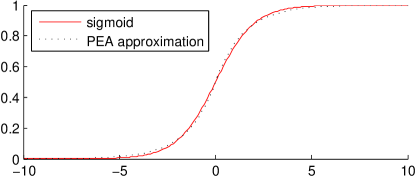
Figure 0.C.1: Piecewise exponential approximation [2] of logistic cdf, equal to the Laplace cdf with scale $1/\log 2$.

We evaluated different approximations AP1, Eq. AP2a,Eq. AP2b and Eq. PEA in Fig. 0.C.2 by measuring the forward KL divergence to the true posterior distribution (computed by convolving densities). We compare to the sampling-based approximation. The results indicate that the baseline AP1 can be significantly improved and that our approximations are on par with sampling.

0.C.4 Variance of Logistic Transform

For the approximation of the mean we can use the same expression as for Logistic Bernoulli, e.g., recall (AP2b) is $\mu^{\prime}=\mathcal{S}(\mu/s)$, where $s=(\sigma^{2}/\sigma^{2}_{\mathcal{S}}+1)^{\frac{1}{2}}$.

The approximation of the variance is more involved in this case. There is no tractable analytic expression for the second moment assuming either normal or logistic distribution of $X$. The approximation of variance based on PEA [2, eq.14] was found inaccurate for small $\sigma$ and because it makes a heavy use of error functions (that can only be approximated with series) is numerically unstable for a wider range of parameters.

Practical Approximation

We have constructed the following practical approximation:

$$\sigma^{\prime 2}\approx{\textstyle 4}(1+4\sigma^{-2})^{-1}(\mu^{\prime}(1-\mu^{\prime}))^{2}.$$ (33)

It is set up to match the following asymptotes. Note that for $\mu=0$, there holds $(\mu^{\prime}(1-\mu^{\prime}))^{2}=1/16$ for all $\sigma$. Then for $\mu=0$ and $\sigma^{2}\rightarrow\infty$ it must be $\sigma^{\prime 2}={\textstyle\frac{1}{4}}$: we can think of this limit as rescaling the sigmoid function, which approaches then the Heaviside step function, which has variance $\frac{1}{4}$ at $\mu=0$. Another asymptote is for $\sigma^{2}\rightarrow 0$, where the variance should approach that of the linearized model with the slope given by the derivative of the logistic function at $\mu=0$. This is satisfied since $\mu^{\prime}$ approaches $\mathcal{S}(\mu)$ and the derivative of the logistic function can be written as $\mathcal{S}(\mu)(1-\mathcal{S}(\mu))$. The variance is then proportional to the square of the derivative. Thus, the model (33) is designed to be accurate for small $\sigma$. For $\mu=0$ the maximum relative error in $\sigma^{\prime}$ is $14\%$ for the whole range of $\sigma$ (numerical simulations). For $\sigma\leq 1$ the maximum relative error is $26\%$ for all $\mu$, more accurate for smaller $\sigma$. For $\sigma>1$ the approximation degrades slowly.

Approximation for Large Variance

For $\sigma\geq 2$, the following approximation is more accurate. In order to compute $E_{X}\mathcal{S}^{2}(X)$ we apply the same trick as with expectation of $\mathcal{S}(X)$. Observe that $\mathcal{S}^{2}(X)$ can be considered as a cdf and let $Z$ have this distribution. Then $E_{X}\mathcal{S}^{2}(X)=E_{X,Z}\mathchoice{\hbox to0.0pt{$\displaystyle{[}$\hss}}{\hbox to0.0pt{$\textstyle{[}$\hss}}{\hbox to0.0pt{$\scriptstyle{[}$\hss}}{\hbox to0.0pt{$\scriptscriptstyle{[}$\hss}}\hskip 1.3pt[X-Z\geq 0]\hskip 1.36pt\mathchoice{\hbox to0.0pt{\hss$\displaystyle{]}$}}{\hbox to0.0pt{\hss$\textstyle{]}$}}{\hbox to0.0pt{\hss$\scriptstyle{]}$}}{\hbox to0.0pt{\hss$\scriptscriptstyle{]}$}}$. We calculate that $\mu^{Z}=1$ and $\sigma^{Z}=(\pi^{2}/3-1)^{\frac{1}{2}}$. Assuming that $X-Z$ is distributed normally with mean $\mu^{X}-1$ and variance $(\sigma^{X})^{2}+\pi^{2}/3-1$ we get the approximation for the variance

$$\Phi\big{(}(\mu-1)/(\sigma^{2}+\sigma_{\mathcal{S}}^{2}-1)^{\frac{1}{2}}\big{)}-\mu^{\prime 2}.$$ (34)

This is not directly usable in practice because of the error functions and needs to be approximated further.

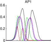
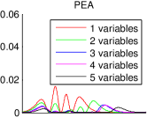
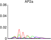
Figure 0.C.2: Comparison of approximations for logistic unit in Fig. 0.C.3. Each line shows KL divergence to the true posterior (in bits) as a function of the bias. Curves are plotted for 1-5 input variables $X_{i}$. Note the 10-fold scaling of y-axis of AP1 compared to others. Note that all approximations: PEA and AP2a, AP2b achieve about the same accuracy in this test, comparable to the estimate using 50 samples (solid lines show mean KL divergence over 1000 repeated trials, dashed lines show 90 percent confidence interval of the trials).

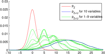
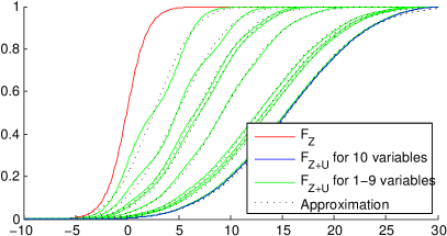
$w=(5.1,4.6,3.5,0.9,4.3,7.0,1.1,0.7,3.6,0.3)$

Figure 0.C.3: Illustration to Proposition 1: an example of the distribution of the sum $U+Z$, where $U=\sum_{i=1}^{n}w_{i}X_{i}$ for 1 to $10$ independent Bernoulli variables $X_{i}$ with $p(X_{i}{=}1)=0.5$ and $Z$ has a logistic distribution. Weights $w$ are displayed in the bottom (drawn once from $U[0,10]$). Left: densities. With $2$ inputs the distribution is bimodal, but with more inputs it quickly tends to normality. Right: cdfs of $Z$ and $Z+U$ and the approximating normal cdf Eq. AP2a. Note that due to the symmetry of the Logistic density, $U+Z$ and $U-Z$ have identical distributions.

0.C.5 ReLU

The mean of $\max(0,X)$ expresses as

$$\mu^{\prime}=\int_{-\infty}^{\infty}\max(0,x)p(x){\rm d}x=\int_{0}^{\infty}xp(x){\rm d}x.$$ (35)

Consequently, assuming $X$ to be normally distributed, we get

$$\int_{0}^{\infty}x\phi((x-\mu)/\sigma){\rm d}x=\int_{-\mu/\sigma}^{\infty}(\mu+\sigma x)\phi(x){\rm d}x$$ (36)

$$=\mu\int_{-\mu/\sigma}^{\infty}\phi(x){\rm d}x-\sigma\int_{-\mu/\sigma}^{\infty}\phi^{\prime}(x){\rm d}x$$ (37)

$$=\mu\Phi(\mu/\sigma)+\sigma\phi(\mu/\sigma).$$ (38)

where we used that $x\phi(x)=\phi^{\prime}(x)$ holds for the pdf of the standard normal distribution,

Second moment:

$$\int_{0}^{\infty}x^{2}\phi((x-\mu)/\sigma){\rm d}x=\int_{-\mu/\sigma}^{\infty}(\sigma x+\mu)^{2}\phi(x){\rm d}x$$ (39)

$$=\int_{-\mu/\sigma}^{\infty}(\sigma^{2}x^{2}+2\sigma\mu x+\mu^{2})\phi(x){\rm d}x$$ (40)

$$=\sigma^{2}\int_{-\mu/\sigma}^{\infty}-x\phi^{\prime}(x){\rm d}x+2\sigma\mu\phi(\mu/\sigma)+\mu^{2}\Phi(\mu/\sigma)$$

$$=\sigma^{2}\Big{(}\frac{\mu}{\sigma}\phi\left(\frac{-\mu}{\sigma}\right)+\Phi\left(\frac{\mu}{\sigma}\right)\Big{)}+2\sigma\mu\phi\left(\frac{\mu}{\sigma}\right)+\mu^{2}\Phi\left(\frac{\mu}{\sigma}\right)$$

$$=\sigma\mu\phi(\mu/\sigma)+(\mu^{2}+\sigma^{2})\Phi(\mu/\sigma).$$ (41)

Let us denote $a=\mu/\sigma$. Then $\mu^{\prime}=\sigma(a\Phi(a)+\phi(a))$. The variance in turn expresses as

$$\sigma^{\prime 2}=\sigma^{2}\mathcal{R}(a),$$ (42)

where

$$\mathcal{R}(a)=a\phi(a)+(a^{2}+1)\Phi(a)-(a\Phi(a)+\phi(a))^{2}.$$ (43)

This function is non-negative by the definition of variance. However it contains positive and negative terms and in a numerical approximation the errors may not cancel and result in a negative value. In practice this function of one variable can be well-approximated by a single logistic function, and guaranteed to be non-negative in this way.

Logistic approximations are computed with Mathematica. The two approximations for the mean are illustrated in Fig. 0.C.4. The logistic approximation of the mean was also given in [3, Prop.1]. The two approximations appear very similar. ELU activation [4] can be also seen as an approximation of the expectation, if we disregard the horizontal and vertical offsets, which can be influenced by the biases before and after the non-linearity.

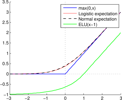
Figure 0.C.4: The mean of $\max(0,X)$, under the approximation that $X$ is distributed Normally or logistically, in both cases with variance 1. The two approximations are very similar. For comparison also the ELU activation [4] is shown, with an input offset by 1.

0.C.6 Max and Leaky ReLU

We will consider the function $\max(X_{1},X_{2})$ in the two special cases: when $X_{2}=\alpha X_{1}$, i.e., they are fully correlated, and when $X_{1}$ and $X_{2}$ are assumed independent. The first case is useful for representing leaky ReLU, given by $\max(X,\alpha X)$ and the second case may be used to handle cases where we don’t know the correlation, e.g. max pooling and maxOut. We use moments for the maximum of two correlated Gaussian random variables given in [23]. Denoting $s=(\sigma_{1}^{2}+\sigma_{2}^{2}-2\operatorname{Cov}[X_{1},X_{2}])^{\frac{1}{2}}$ and $a=(\mu_{1}{-}\mu_{2})/s$, the mean and variance of $\max(X_{1},X_{2})$ can be expressed as:

$$\mu^{\prime} =\mu_{1}\Phi(a)+\mu_{2}\Phi(-a)+s\phi(a),$$ (44a)

$$\sigma^{\prime 2} \begin{aligned} =\>&(\sigma_{1}^{2}+\mu_{1}^{2})\Phi(x)+(\sigma_{2}^{2}+\mu_{2}^{2})\Phi(-a)\\ +\>&(\mu_{1}+\mu_{2})s\phi(a)-\mu^{\prime 2}.\end{aligned}$$ (44b)

The mean can be expressed as:

$$\mu^{\prime}=\mu_{2}+s\big{(}a\Phi(a)+\phi(a)\big{)}.$$ (45)

Substituting this expression into (44b) we obtain

$$\sigma^{\prime 2}=\sigma_{1}^{2}\Phi(a)+\sigma_{2}^{2}\Phi(-a)+s^{2}(a^{2}\Phi(a)+a\phi(a)-(a\Phi(a)+\phi(a))^{2})$$ (46)

Reusing the function $\mathcal{R}$ (43), the variance expresses as:

$$\sigma^{\prime 2}=\sigma_{1}^{2}\Phi(a)+\sigma_{2}^{2}\Phi(-a)+s^{2}(\mathcal{R}(a)-\Phi(a)).$$ (47)

Leaky ReLU

We now can derive a simplified expression for LReLU. Assume that $\alpha<1$, let $X_{2}=\alpha X_{1}$ and denote $\mu=\mu_{1}$ and $\sigma^{2}=\sigma_{1}^{2}$. Then $\mu_{2}=\alpha\mu$, $\sigma_{2}^{2}=\alpha^{2}\sigma^{2}$ and $\operatorname{Cov}[X_{1},X_{2}]=\operatorname{Cov}[X_{1},\alpha X_{1}]=\alpha\sigma^{2}$. We then have $s=\sigma(1-\alpha)$ and $a=(\mu_{1}-\mu_{2})/s=\mu(1-\alpha)/s=\mu/\sigma$. The mean $\mu^{\prime}$ expresses as

$$\mu^{\prime}=\mu(\alpha+(1-\alpha)\Phi(a))+\sigma(1-\alpha)\phi(a).$$ (48)

The variance $\sigma^{\prime 2}$ expresses as

$$\sigma^{2}\Big{(}\Phi(a)+\alpha^{2}(1-\Phi(a))+(1-\alpha)^{2}\big{(}a^{2}\Phi(a)+a\phi(a)-(a\Phi(a)+\phi(a))^{2}\big{)}\Big{)}$$ (49)

$$=\sigma^{2}(\alpha^{2}+2\alpha(1-\alpha)\Phi(a)+(1-\alpha)^{2}\mathcal{R}(a)).$$ (50)

In practice we approximate it with the function

$$\sigma^{\prime 2}\approx\sigma^{2}(\alpha^{2}+(1-\alpha^{2})\mathcal{S}(a/t)),$$ (51)

where $t$ is set by fitting the approximation (see § 0.D.1). The approximation is shown in Fig. 3.

Uncorrelated Case

In this case we have $s^{2}=\sigma_{1}^{2}+\sigma_{2}^{2}$. The expression for the variance (46) can be written as

$$\sigma^{\prime 2}=\sigma_{1}^{2}\mathcal{R}(a)+\sigma_{2}^{2}(\Phi(-a)+\mathcal{R}(a)-\Phi(a)).$$ (52)

This expression can be well approximated with

$$\sigma_{1}^{2}\mathcal{S}(a/t)+\sigma_{2}^{2}\mathcal{S}(-a/t)$$ (53)

with a suitable parameter $t$. For the purpose of visualization, consider applying this approximation for computing the moments of $\max(X,\alpha X)$, ignoring the correlation. It will result in a plot similar to Fig. 3 but with a slightly increased variance in the transition part and with a slightly more smoothed mean.

0.C.7 Softmax

For the posterior of softmax $p(Y{=}y\,|\,X)=\exp(X_{y})/\sum_{i}\exp(X_{i})$ we need to estimate

$$\mathbb{E}_{X}\Big{[}\frac{e^{X_{y}}}{\sum_{k}e^{X_{k}}}\Big{]}=\mathbb{E}_{X}\Big{[}\frac{1}{1+\sum_{k\neq y}e^{X_{k}-X_{y}}}\Big{]}.$$ (54)

Let $U_{k}=X_{y}-X_{k}$ for $k\neq y$, so that $U$ is a r.v. in $\mathbb{R}^{n-1}$. Let us assume for simplicity that $y=n$. Expression (54) can be written as

$$\mathbb{E}_{U}\Big{[}\big{(}\textstyle 1+\sum_{k<n}e^{-U_{k}}\big{)}^{-1}\Big{]}=\mathbb{E}_{U}[\mathcal{S}_{n-1}(U)],$$ (55)

where $\mathcal{S}_{n-1}$ is the cdf of the $(n{-}1)$-variate logistic distribution [20, eq. 2.5]:

$$\mathcal{S}_{n-1}(u)=\frac{1}{1+\sum_{k}e^{-u_{k}}}.$$ (56)

We can apply the same trick as in Observation 1. Let $Z\sim\mathcal{S}_{n-1}$. Then

$$\mathbb{E}_{U}\mathcal{S}_{n-1}(U)=\mathbb{E}_{U,Z}\mathchoice{\hbox to0.0pt{$\displaystyle{[}$\hss}}{\hbox to0.0pt{$\textstyle{[}$\hss}}{\hbox to0.0pt{$\scriptstyle{[}$\hss}}{\hbox to0.0pt{$\scriptscriptstyle{[}$\hss}}\hskip 1.3pt[U-Z\geq 0]\hskip 1.36pt\mathchoice{\hbox to0.0pt{\hss$\displaystyle{]}$}}{\hbox to0.0pt{\hss$\textstyle{]}$}}{\hbox to0.0pt{\hss$\scriptstyle{]}$}}{\hbox to0.0pt{\hss$\scriptscriptstyle{]}$}}.$$ (57)

For multi-variate logistic distribution of $Z$, the marginal distribution of $Z_{k}$ is logistic [20], hence we know $Z_{k}$ has mean $0$ and variance $\sigma_{S}^{2}$. We can thus express the mean of $(U-Z)_{k}$ as $\tilde{\mu}_{k}=\mu_{y}-\mu_{k}$ and its variance as $\tilde{\sigma}^{2}_{k}=\sigma^{2}_{y}+\sigma^{2}_{k}+\sigma_{S}^{2}$ (this relies only on that $X_{y}$, $X_{k}$ and $Z_{k}$ are independent). Note in, general, the components of $U-Z$ are not independent.

The normal approximation, similar to Eq. AP2a is as follows. Assuming that $U-Z$ has multivariate normal distribution with diagonal covariance (which implies that the components of $U-Z$ are independent), gives the approximation:

$$q(y)=\Pr\{U{-}Z\geq 0\}\approx\prod_{k\neq y}\Phi\Big{(}\frac{\tilde{\mu}_{k}}{\tilde{\sigma}_{k}}\Big{)}.$$ (58)

Expanding, we obtain

$$q(y)\approx\prod_{k\neq y}\Phi\Big{(}\frac{\mu_{y}-\mu_{k}}{\sqrt{\sigma^{2}_{y}+\sigma^{2}_{k}+\sigma_{S}^{2}}}\Big{)}.$$ (59)

The logistic approximation, similar to Eq. AP2b is as follows. Assuming that $U-Z$ has multivariate logistic distribution with the matching mean and the diagonal elements of the covariance matrix, we can approximate

$$q(y)\approx\mathcal{S}_{n-1}\big{(}\{\tilde{\mu}_{k}/(\tilde{\sigma}_{k}/\sigma_{\mathcal{S}})\}_{k}\big{)}.$$ (60)

Expanding, we obtain the approximation

$$q(y)\approx\Big{(}1+\sum_{k\neq y}\exp\Big{\{}\frac{\mu_{k}-\mu_{y}}{\textstyle\sqrt{(\sigma^{2}_{k}+\sigma^{2}_{y})/\sigma^{2}_{\mathcal{S}}+1}}\Big{\}}\Big{)}^{-1}.$$ (61)

In both cases, a renormalization of $q$ is needed in order to ensure a proper distribution. This is not guaranteed by the approximation as was the case with (AP2a), (AP2b). Approximation (61) can be implemented in the logarithmic domain as follows:

$$\log q(y):=-\operatorname{logsumexp}_{k}\frac{\mu_{k}-\mu_{y}}{\sqrt{(\sigma_{k}^{2}+\sigma_{y}^{2})/\sigma_{S}^{2}+1}},$$ (62)

where $\operatorname{logsumexp}_{k}$ is $\log\sum_{k}\exp$ operation. This can be done in quadratic time and with linear memory complexity. The renormalization of $q$ in the logarithmic domain takes the form

$$\log q(y):=\log q(y)-\operatorname{logsumexp}_{k}\log q(k).$$ (63)

The log likelihood (12) can take $\log q(y)$ directly, avoiding the exponentiation, as with regular softmax. It turned out that back propagation through this softmax was rather slow and we replaced it with a simplified approximation

$$\log q(y):=-\operatorname{logsumexp}_{k}\Big{(}\frac{\mu_{k}}{\sqrt{\sigma_{k}^{2}/\sigma_{S}^{2}+1}}-\frac{\mu_{y}}{\sqrt{\smash[b]{\sigma_{y}^{2}}/\sigma_{S}^{2}+1}}\Big{)},$$ (64)

which reduces to standard softmax of $\mu_{k}/\sqrt{\sigma_{k}^{2}/\sigma_{S}^{2}+1}$. There is a noticeable loss of accuracy in the KL divergence of the posterior distribution seen in the experiments (Tables 2 and 3), which is however not critical. We therefore used this expression in the end-to-end training experiments.

Connection to argmax

We now explain a refinement of the latent variable model for softmax, which allows to see its interpretation as the expected value of $\mathop{\rm argmax}$. In fact, this interpretation is well known in particular in the multinational logistic regression, we just expose the relation between these models.

As mentioned above, the components of $Z$ following the $(n-1)$-variate logistic distribution are not independent, but they have the following latent variable representation [20, eq. 2.1-2.4]. Let $\alpha$ has the exponential density function $e^{-\alpha}$, $\alpha>0$. Let variables $Z_{i}$ given $\alpha$ be independent with the conditional distribution

$$F_{Z_{k}\,|\,\alpha}(z)=e^{-\alpha e^{-z}}.$$ (65)

Then the joint marginal distribution of $Z$ is the multivariate logistic distribution $\mathcal{S}_{n-1}$. This latent variable model can in turn be rewritten in the following form, very suitable for our purpose.

Lemma 0.C.1.

Let $V_{i}$ be independent r.v.’s with the exponential density $p_{V_{i}}(u)=e^{-u}$, $u>0$. Let $Z_{i}=\log(V_{n})-\log(V_{i})$ for i = $1,\dots,n-1$. Then $Z$ has $(n{-}1)$-variate logistic distribution.

Proof.

It can be verified that the cdf of $-\log(V_{i})$ expresses as $F_{-\log(V_{i})}(u)=$

$$Pr\{-\log(V_{i})\leq u\}=Pr\{V_{i}\geq e^{-u}\}=\int_{e^{-u}}^{\infty}e^{-x}dx=e^{-e^{-u}}.$$ (66)

The conditional cdf of $Z_{i}$ given $V_{n}=\alpha$, in turn expresses as

$$F_{Z_{i}}(z)=Pr\{\log(\alpha)-\log(V_{i})\leq z\}=F_{-\log(V_{i})}(z-\log(\alpha))$$ (67)

$$=e^{-e^{-z+\log(\alpha)}}=e^{-\alpha e^{-z}},$$ (68)

which matches (65). ∎

In combination with (55), the softmax has a latent variable formulation $p(Y{=}y\,|\,X=x)=$

$$\mathbb{E}\big{[}x_{y}-x_{k}-Z_{k}\geq 0\ \forall k\big{]}=\mathbb{E}\big{[}x_{y}-\log V_{y}-(x_{k}-\log V_{k})\geq 0\ \forall k\big{]}$$ (69)

$$= \mathbb{E}\big{[}x_{y}+\Gamma_{y}\geq x_{k}+\Gamma_{k}\ \forall k\big{]},$$

where $\Gamma_{k}=-\log V_{k}$ for $k=1,\dots n$ are independent noises with cdf (66) known as Gumbel or type I extreme value distribution. It follows that the softmax model $p(Y\,|\,X)$ can be equivalently defined as

$$Y=\mathop{\rm argmax}_{k}(X_{k}+\Gamma_{k}).$$ (70)

Denoting $\tilde{X}_{k}=X_{k}+\Gamma_{k}$ the (additionally) noised input variables, we can express

$$p(Y{=}y)=\mathbb{E}\big{[}p(Y{=}y\,|\,X)\big{]}=\mathbb{E}\Big{[}\mathop{\rm argmax}_{k}\tilde{X}_{k}=y\Big{]}.$$ (71)

Therefore the problem of computing the expectation of softmax has been reduced to computing the expectation of $\arg\max$ for additionally noised inputs. This connection is very similar to how expectation of sigmoid function was reduced to the expectation of the Heaviside step function with additional injected noise input.

0.C.8 Probit

Let us consider probit model: $Y$ is a Bernoulli r.v. with $p(Y{=}1\,|\,X)=\Phi(X)$. It has the latent variable interpretation $Y=X-Z$, $Z\sim\Phi$. In our approximation Eq. AP2a it changes only the value of noise variance, which gives a simplified formula

$$\mathbb{E}[\Phi(X)]\approx\Phi\Big{(}\frac{\mu}{\sqrt{\sigma^{2}+1}}\Big{)}.$$ (72)

Note that the approximation that $X-Z$ is normally distributed becomes more plausible.

Appendix 0.D Experiment Details

In this section we give all details necessary to ensure reproducibility of results and auxiliary plots giving more details on the experiments in the main part.

0.D.1 Implementation Details

We implemented our inference and learning in the pytorch framework. The source code will be published together with the paper. The implementation contains a number of layers Linear, Conv2D, Sigmoid, ReLU, SoftMax, Normalize, etc., that input and output a pair of mean and variance and can be easily used to upgrade a standard model made of such layers. At present we use only higher-level pytorch functions to implement these layers. For example, convolutional layer is implemented simply as

⬇

y.mean = F.conv2d(x.mean, w) + b

y.var = F.conv2d(x.var, w*w)

The ReLU variance function $\mathcal{R}(x)$ (43), which is also used in leaky ReLU, was approximated by a single logistic function

⬇

F.sigmoid(x /0.3729)

fitted to minimize the maximum KL divergence for LReLU(0.01). The cdf of the normal distribution was approximated by the cdf of the logistic distribution as $\Phi(x)\approx\mathcal{S}(x\pi/\sqrt{3})$, i.e., by matching the variance. Under this approximation the means of logistic-Bernoulli and logistic transform are the same for bith (AP2a) and (AP2b). For the variance of logistic transform we used the expression (33).

For numerical stability, it was essential that $\operatorname{logsumexp}$ is implemented by subtracting the maximum value before exponentiation

⬇

m, _ = x.max()

m = m.detach() # does not influence gradient

y = m + torch.log(torch.sum(torch.exp(x - m)))

The relative times of a forward-backward computation in our higher-level implementation are as follows:

⬇

standard training 1

BN 1.5

inference=AP2 3

inference=AP2-norm=AP2 6

Please note that these times hold for unoptimized implementations. In particular, the computational cost of the AP2 normalization, which propagates the statistics of a single pixel statistics, should be negligible in comparison to propagating a batch of input images.

0.D.2 Parameters

We used batch size 128, Adam optimizer with learning rate $10^{-3}0.06^{k}$, where $k$ is the epoch number. This schedule smoothly decreases the learning rate by about order of 10 every 50 epochs. Parameters of linear and convolutional layers were initialized using pytorch defaults, i.e., uniformly distributed in $[-1/\sqrt{c},\,1/\sqrt{c}]$, where c is the number of inputs per one output. All experiments use a fixed random seed so that the initial point is the same. The results were fairly repeatable with arbitrary seeds.

0.D.3 Datasets

We used MNIST and CIFAR10 datasets. Both datasets provide a split into training and test sets. From the training set we split 10 percent (at random) to create a validation set. The validation set is meant for model selection and monitoring the validation loss and accuracy during learning. The test sets were currently used only in the stability tests.

0.D.4 Network specifications

The MNIST single hidden layer network in § 4 MLP/MNIST has the architecture: input - FC 784x100 - Norm - Logistic Bernoulli - FC 100 x10 - Norm - Softmax, where Norm may be none, BN, AP2. With the normalization switched on, the biases of linear layers preceding normalizations are turned off.

The LeNet in § 4 has the structure:

⬇

Conv2d(1, 32, ks=5, st=2), Norm, Activation

Conv2d(32, 64, ks=5, st=2), Norm, Activation

Conv2d(64, 50, ks=4), Norm, Activation

Conv2d(50, 10, ks=1), Norm, LogSoftmax

Convolutional layer parameters list input channels, output channels, kernel size and stride. Dropout layers are inserted after activations.

The CIFAR network in § 4 has a structure similar to LeNet with the following conv layers:

⬇

ksize = [3, 3, 3, 3, 3, 3, 3, 1, 1 ]

stride= [1, 1, 2, 1, 1, 2, 1, 1, 1 ]

depth = [96, 96, 96, 192, 192, 192, 192, 192, 10]

each but the last one ending with Norm and activation. The final layers of the network are

⬇

Norm, AdaptiveAvgPool2d, LogSoftmax

0.D.5 Additional Experimental Results

Stability to Adversarial Attacks

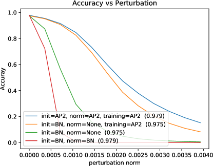
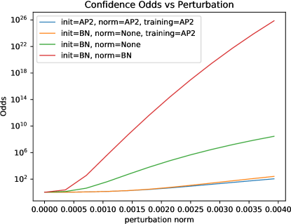
Figure 0.D.1: Stability evaluation of MLP/MNIST model under gradient sign attack. Left: test accuracy versus the maximum allowed norm of the adversarial perturbation who’s direction is tailored per image. Right confidence odds as in Fig. 5.

References

- Arpit et al. [2016] Arpit, D., Zhou, Y., Kota, B.U., Govindaraju, V.: Normalization propagation: A parametric technique for removing internal covariate shift in deep networks. In: Balcan, M., Weinberger, K.Q. (eds.) ICML. JMLR Workshop and Conference Proceedings, vol. 48, pp. 1168–1176. JMLR.org (2016), http://jmlr.org/proceedings/papers/v48/arpitb16.html
- Astudillo and da Silva Neto [2011] Astudillo, R.F., da Silva Neto, J.P.: Propagation of uncertainty through multilayer perceptrons for robust automatic speech recognition. In: INTERSPEECH (2011)
- Bengio et al. [2013] Bengio, Y., Léonard, N., Courville, A.C.: Estimating or propagating gradients through stochastic neurons for conditional computation. CoRR abs/1308.3432 (2013)
- Clevert et al. [2015] Clevert, D.A., Unterthiner, T., Hochreiter, S.: Fast and accurate deep network learning by exponential linear units (ELUs). CoRR abs/1511.07289 (2015)
- Dayan et al. [1995] Dayan, P., Hinton, G.E., Neal, R.N., Zemel, R.S.: The Helmholtz machine. Neural Computation 7, 889–904 (1995)
- Fawzi et al. [2016] Fawzi, A., Moosavi-Dezfooli, S.M., Frossard, P.: Robustness of classifiers: from adversarial to random noise. In: NIPS, pp. 1632–1640 (2016)
- Flach et al. [2017] Flach, B., Shekhovtsov, A., Fikar, O.: Generative learning for deep networks. CoRR abs/1709.08524 (2017)
- Frey and Hinton [1999] Frey, B.J., Hinton, G.E.: Variational learning in nonlinear gaussian belief networks. Neural Comput. 11(1), 193–213 (Jan 1999)
- Goodfellow et al. [2015] Goodfellow, I., Shlens, J., Szegedy, C.: Explaining and harnessing adversarial examples. In: International Conference on Learning Representations (2015), http://arxiv.org/abs/1412.6572
- Hernández-Lobato and Adams [2015] Hernández-Lobato, J.M., Adams, R.P.: Probabilistic backpropagation for scalable learning of Bayesian neural networks. In: ICML. pp. 1861–1869 (2015)
- Ioffe and Szegedy [2015] Ioffe, S., Szegedy, C.: Batch normalization: Accelerating deep network training by reducing internal covariate shift. In: ICML. vol. 37, pp. 448–456 (2015)
- Kingma [2013] Kingma, D.P.: Fast gradient-based inference with continuous latent variable models in auxiliary form. CoRR abs/1306.0733 (2013)
- Kingma and Ba [2014] Kingma, D.P., Ba, J.: Adam: A method for stochastic optimization. CoRR abs/1412.6980 (2014), http://arxiv.org/abs/1412.6980
- Kingma et al. [2015] Kingma, D.P., Salimans, T., Welling, M.: Variational dropout and the local reparameterization trick. In: Advances in Neural Information Processing Systems 28, pp. 2575–2583 (2015)
- Kingma and Welling [2014a] Kingma, D.P., Welling, M.: Efficient gradient-based inference through transformations between Bayes nets and neural nets. In: ICML. pp. II–1782–II–1790 (2014a), http://dl.acm.org/citation.cfm?id=3044805.3045091
- Kingma and Welling [2014b] Kingma, D.P., Welling, M.: Efficient gradient-based inference through transformations between Bayes nets and neural nets. In: ICML. pp. II–1782–II–1790. ICML’14, JMLR.org (2014b), http://dl.acm.org/citation.cfm?id=3044805.3045091
- Klambauer et al. [2017] Klambauer, G., Unterthiner, T., Mayr, A., Hochreiter, S.: Self-normalizing neural networks. CoRR abs/1706.02515 (2017)
- MacKay [1992a] MacKay, D.J.C.: The evidence framework applied to classification networks. Neural Computation 4(5), 720–736 (Sept 1992a)
- MacKay [1992b] MacKay, D.J.C.: A practical Bayesian framework for backpropagation networks. Neural Comput. 4(3), 448–472 (May 1992b), http://dx.doi.org/10.1162/neco.1992.4.3.448
- Malik and Abraham [1973] Malik, H.J., Abraham, B.: Multivariate logistic distributions. The Annals of Statistics 1(3), 588–590 (1973), http://www.jstor.org/stable/2958123
- Minka [2001] Minka, T.P.: Expectation propagation for approximate Bayesian inference. In: Uncertainty in Artificial Intelligence. pp. 362–369 (2001)
- Moosavi-Dezfooli et al. [2017] Moosavi-Dezfooli, S.M., Fawzi, A., Fawzi, O., Frossard, P.: Universal adversarial perturbations. In: CVPR (July 2017)
- Nadarajah and Kotz [2008] Nadarajah, S., Kotz, S.: Exact distribution of the max/min of two gaussian random variables. IEEE Trans. VLSI Syst. 16(2), 210–212 (2008)
- Neal [1992] Neal, R.M.: Connectionist learning of belief networks. Artif. Intell. 56(1), 71–113 (Jul 1992)
- Nguyen et al. [2015] Nguyen, A., Yosinski, J., Clune, J.: Deep neural networks are easily fooled: High confidence predictions for unrecognizable images. In: CVPR (2015)
- Papaspiliopoulos et al. [2007] Papaspiliopoulos, O., Roberts, G.O., Sk ld, M.: A general framework for the parametrization of hierarchical models. Statist. Sci. 22(1), 59–73 (02 2007), http://dx.doi.org/10.1214/088342307000000014
- Pearl [1988] Pearl, J.: Probabilistic Reasoning in Intelligent Systems: Networks of Plausible Inference (1988)
- Rezende et al. [2014] Rezende, D.J., Mohamed, S., Wierstra, D.: Stochastic backpropagation and approximate inference in deep generative models. In: ICML. vol. 32, pp. 1278–1286 (2014)
- Rodner et al. [2016] Rodner, E., Simon, M., Fisher, B., Denzler, J.: Fine-grained recognition in the noisy wild: Sensitivity analysis of convolutional neural networks approaches. In: BMVC (2016)
- Salimans and Kingma [2016] Salimans, T., Kingma, D.P.: Weight normalization: A simple reparameterization to accelerate training of deep neural networks. In: NIPS (2016)
- Schoenholz et al. [2016] Schoenholz, S.S., Gilmer, J., Ganguli, S., Sohl-Dickstein, J.: Deep information propagation. CoRR abs/1611.01232 (2016)
- Shekhovtsov and Flach [2018] Shekhovtsov, A., Flach, B.: Normalization of neural networks using analytic variance propagation. In: CVWW (2018)
- Srivastava et al. [2014] Srivastava, N., Hinton, G., Krizhevsky, A., Sutskever, I., Salakhutdinov, R.: Dropout: A simple way to prevent neural networks from overfitting. Journal of Machine Learning Research 15, 1929–1958 (2014), http://jmlr.org/papers/v15/srivastava14a.html
- Szegedy et al. [2014] Szegedy, C., Zaremba, W., Sutskever, I., Bruna, J., Erhan, D., Goodfellow, I., Fergus, R.: Intriguing properties of neural networks. In: International Conference on Learning Representations (2014), http://arxiv.org/abs/1312.6199
- Wang and Manning [2013] Wang, S., Manning, C.: Fast dropout training. In: ICML. pp. 118–126 (2013)
- Williams [1992] Williams, R.J.: Simple statistical gradient-following algorithms for connectionist reinforcement learning. Machine Learning 8(3), 229–256 (May 1992), https://doi.org/10.1007/BF00992696
Appendix \@starttoctoc