Quadratic chaotic inflation with a logarithmic-corrected mass

Abstract

We consider a simple modification of quadratic chaotic inflation. We add a logarithmic correction to the mass term, and find that this model can be consistent with the latest cosmological observations such as the Planck 2018 data, in combination with the BICEP2/Keck Array and the baryon acoustic oscillation data. Since the model predicts the lower limit for the tensor-to-scalar ratio $r$ for the present allowed values of the spectral index $n_{s}$, it could be tested by the cosmic microwave background polarization observation in the near future. In addition, we consider higher-order logarithmic corrections. Interestingly, we observe that the scalar spectral index $n_{s}$ and $r$ stay in rather a narrow region of the parameter space. Moreover, they reside in a completely different region from that for the logarithmic corrections to the quartic coupling. Therefore, future observations may distinguish which kind of corrections should be included, or even single out the form of the interactions.

I Introduction

Inflation is an interesting paradigm in the early Universe. It solves the problems in the hot big bang Universe and may also provide the seeds of the density perturbations of the Universe. The simplest inflation model with a scalar field $\phi$ would be chaotic inflation Linde with a quadratic potential,

$$V=\frac{1}{2}m^{2}\phi^{2},$$ (1)

where $m$ is the mass of the scalar field $\phi$. However, this simple model is likely be excluded by recent observations such as the cosmic microwave background (CMB) observations by the Planck satellite Planck . The main obstacle is that the tensor perturbations it predicts are too large because of the large potential energy at the large field amplitudes during inflation.

One way out is to somehow lower the potential at large field values. A lot of scenarios along this line have been proposed rad1 ; rad2 ; rad3 ; poly1 ; poly2 ; poly3 ; nonK1 ; nonK2 ; nonK3 ; nonK4 ; nonG1 ; nonG2 ; nonG3 ; nonG4 ; nonG5 ; nonG6 ; otherfield1 ; otherfield2 ; R1 ; R2 ; R3 . An interesting possibility is due to radiative corrections rad1 ; rad2 ; rad3 , where, in most cases, the quadratic potential becomes flatter because of the running of the quartic coupling of the inflaton.

In this article, we instead consider a very simple case where the mass has a running of the following form:

$$m^{2}(\phi)=m^{2}\left[1-K\log\frac{\phi^{2}}{M^{2}}\right],$$ (2)

where $K$ is a positive constant and $M$ is some large mass scale. Positive $K$ can be realized, for example, when couplings of $\phi$ to fermions dominate over those to bosons if the logarithmic correction is radiatively produced. As shown below, we find that the model is consistent with the Planck 2018 data, in combination with the BICEP2/Keck Array (BK14) and the baryon acoustic oscillation (BAO) data Planck . This is contrasted with the corrections due to the running of the quartic coupling, which may now be inconsistent with the combination of the Planck 2018 and BK14/BAO data.

In addition, we go further to include higher-order logarithmic corrections to the mass term. It is interesting to note that the scalar spectral index $n_{s}$ of the curvature perturbation and the tensor-to-scalar ratio $r$ stay in a narrow region of the parameter space ($n_{s}$, $r$), so that we could still find $n_{s}$ and $r$ consistent with the data for slightly different model parameters. For comparison, we investigate higher-order logarithmic corrections to a quartic coupling of the potential, which places $n_{s}$ and $r$ in a completely different region of the parameter space ($n_{s}$, $r$).

Notice that Ref. rad3 considered the radiative corrections to the mass, including the second order of the logarithmic corrections to make a plateau in the potential. We do not consider such particular potentials in this article.

II Logarithmic-corrected mass inflation

As mentioned, we consider a simple correction to the mass in quadratic chaotic inflation, where the potential is given by rad3

$$V(\phi)=\frac{1}{2}m^{2}\left(1-K\log\frac{\phi^{2}}{M^{2}}\right)\phi^{2}.$$ (3)

$M$ can be arbitrary, since the form of the potential does not change when we reparametrize as $M\rightarrow M^{\prime}$, $K\rightarrow K^{\prime}=K/[1-K\log(M^{\prime 2}/M^{2})]$, and $m^{2}\rightarrow m^{\prime 2}=m^{2}[1-K\log(M^{\prime 2}/M^{2})]$. Thus, we set $M=M_{\rm P}$ below without loss of generality, where $M_{\rm P}(=2.4\times 10^{18}$ GeV) is the reduced Planck scale. We also assume that nonrenormalizable higher-order terms, for example, bound the potential from below at larger amplitudes, while they do not affect the dynamics of the inflaton during inflation.

Using the slow-roll parameters

$$\epsilon(\phi)\equiv\frac{1}{2M_{\rm P}^{2}}\left(\frac{V^{\prime}(\phi)}{V(\phi)}\right)^{2},\quad\eta(\phi)\equiv\frac{1}{M_{\rm P}^{2}}\frac{V^{\prime\prime}(\phi)}{V(\phi)},$$ (4)

where a prime denotes a derivative with respective to $\phi$, the scalar spectral index $n_{s}$ of the curvature perturbation and the tensor-to-scalar ratio $r$ are, respectively,

$$n_{s}(\phi) = 1-6\epsilon(\phi)+2\eta(\phi),$$ (5)

$$r(\phi) = 16\epsilon(\phi).$$ (6)

They should be evaluated at $\phi=\phi_{N}$, the field amplitude $N$ $e$-folds before the end of inflation. $\phi_{N}$ is related to $N$ by

$$N=\int_{\phi_{\rm e}}^{\phi_{N}}\frac{1}{M_{\rm P}^{2}}\frac{V(\phi)}{V^{\prime}(\phi)}d\phi,$$ (7)

where $\phi_{\rm e}$ stands for the amplitude of the field at the end of inflation, defined by $|\eta(\phi_{\rm e})|=1$.

We numerically calculate $\phi_{N}$ for fixed $N$ to obtain $n_{s}(\phi_{N})$ and $r(\phi_{N})$ for various values of $K$. The results are shown in Table 1 and Fig. 1. We also plot the 1$\sigma$ and 2$\sigma$ region allowed by Planck results Planck in Fig. 1.

Table 1: $n_{s}$ and $r$ for some values of $K$.

$K$	$\phi_{\rm e}/M_{\rm P}$	$N$	$\phi_{N}/M_{\rm P}$	$n_{s}$	$r$
		50	12.90	0.964	0.122
0.10	1.175	55	13.50	0.967	0.110
		60	14.08	0.970	0.100
		50	11.98	0.964	0.089
0.13	1.096	55	12.49	0.967	0.079
		60	12.98	0.969	0.071
		50	11.55	0.962	0.074
0.14	1.070	55	12.01	0.965	0.067
		60	12.45	0.968	0.057
		50	11.03	0.959	0.057
0.15	1.043	55	11.43	0.961	0.048
		60	11.80	0.964	0.041
		50	10.41	0.953	0.038
0.16	1.017	55	10.74	0.954	0.031
		60	11.03	0.955	0.025

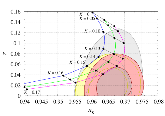
Figure 1: Spectral index $n_{s}$ and tensor-to-scalar ratio $r$ for $K=0-0.17$. The top (blue), middle (green), and bottom (magenta) lines are for $N=50$, 55, and 60, respectively. Notice that the $K=0$ case corresponds to the original quadratic chaotic inflation. The Planck-allowed regions are shown in dark (1$\sigma$) and light (2$\sigma$), where we adopt the Planck TT,TE,EE+lowE+lensing (gray), Planck TT,TE,EE+lowE+lensing+BK14 (yellow), and Planck TT,TE,EE+lowE+lensing+BK14+BAO data (red) Planck .

We can see that the tensor-to-scalar ration $r$ becomes smaller for larger $K$, since the logarithmic term lowers the potential at large amplitudes. For an appropriate range of $K$, the model is consistent with observations. In this model, it is most favorable for $K\simeq 0.14-0.15$ and $N\simeq 55-60$, which resides inside the 1$\sigma$ allowed region for the Planck TT,TE,EE+lowE+lensing data Planck , and is even consistent with the Planck TT,TE,EE+lowE+lensing+BK14+BAO data Planck for $K\simeq 0.14-0.15$ and $N\simeq 60$.

It seems that the tensor-to-scalar ratio $r$ has a lower bound $r\gtrsim 0.02$ for a spectral index $n_{s}$ that is consistent with the Planck observations. Therefore, this model could be tested by the CMB polarization observations in the near future.

III Higher-order corrections

So far we have considered a logarithmic correction to the mass term in the lowest order as in Eq.(2). Here we investigate the effects of including higher-order corrections. To be specific, we expand $m(\phi)$ in powers of log$\phi^{2}$, and assume the following form for the logarithmic corrections to the mass term rad3 :

$$V(\phi)=\frac{1}{2}m^{2}(\phi)\phi^{2}=m^{2}\left[1-K\log\frac{\phi^{2}}{M^{2}}+\sum_{n\geq 2}a_{n}\left(K\log\frac{\phi^{2}}{M^{2}}\right)^{n}\right]\phi^{2},$$ (8)

where the $a_{n}$’s are positive or negative coefficients of order unity. As an example, we calculate $n_{s}$ and $r$ for $N=60$ in the cases of $a_{2}=(-0.4)-0.5$ for $K=0.13$ and $a_{n}=0$ $(n\geq 3)$. The results are shown as the green line in the left panel of Fig. 2. The magenta line denotes the same results as that in Fig. 1, and the black dot represents the original quadratic chaotic inflation. We see that the green line almost coincides with the magenta line.

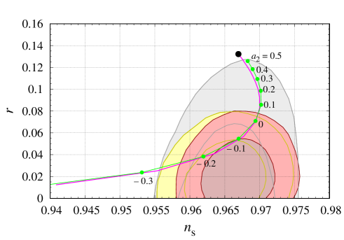
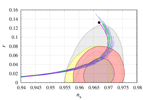
Figure 2: Spectral index $n_{s}$ and tensor-to-scalar ratio $r$ for $N=60$ in the case of the higher-order logarithmic corrections to the mass. The magenta, green, and blue lines represent the cases with corrections up to first, second, and third order, respectively. The black dot denotes the original quadratic chaotic inflation case. The Planck-allowed regions Planck are the same as in Fig. 1. Left: The case for $a_{2}=(-0.4)-0.5$, $K=0.13$ and $a_{n}=0$ $(n\geq 3)$, as an example. Right: All the cases explained in the text.

In order to confirm that this is a generic feature, we estimate the parameters $n_{s}$ and $r$ for the potential (8) up to the second and third orders. We vary the model parameter $a_{2}$ from $-1/2$ to 1/2 for $K=0.13-0.17$ in the former case, while we change $a_{3}$ from $-1/6$ to $1/6$ for $a_{2}=(-0.2)-0.5$ with $K=0.14-0.16$ in the latter case. We show the results for corrections up to first (magenta), second (green), and third (blue) order in the right panel in Fig. 2. We find that the derived parameters $n_{s}$ and $r$ reside in a rather narrow region and are very close to the first-order result, in spite of including the second- and third-order corrections for various values of the model parameters $a_{2}$ and $a_{3}$. We may therefore conclude that the logarithmic corrections to the mass—regardless of their order—make the model consistent with the latest observations such as the Planck TT,TE,EE+lowE+lensing+BK14+BAO data Planck for appropriate coefficients $K$ and $a_{n}$.

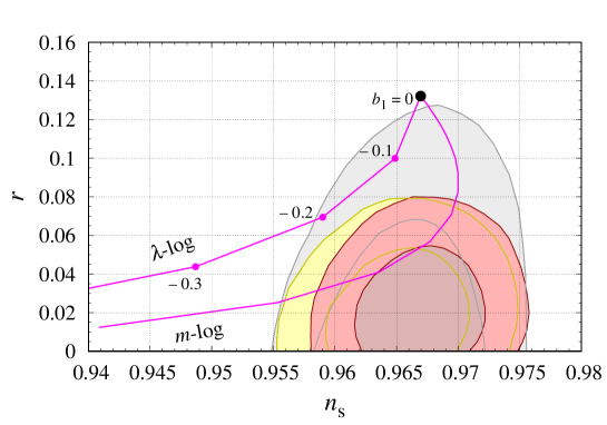
Figure 3: Spectral index $n_{s}$ and tensor-to-scalar ratio $r$ for $N=60$ in the case of the first-order logarithmic corrections to the quartic coupling for $b_{1}=(-0.4)-0$, denoted by the upper magenta line. The lower magenta line denotes the results of the case of the first-order corrections to the mass term as in Fig. 1. The black dot denotes the original quadratic chaotic inflation case. The Planck-allowed regions Planck are the same as in Fig. 1.

For comparison, we also calculate the case with logarithmic corrections to the quartic coupling. The potential is then given by rad1 ; rad2 ; rad3

$$V=\frac{1}{2}m^{2}\phi^{2}+\lambda\left[\sum_{n\geq 1}b_{n}\left(\log\frac{\phi^{2}}{M^{2}}\right)^{n}\right]\phi^{4}.$$ (9)

Here $\lambda\ll 1$ and the $b_{n}$’s are coefficients of $O((0.1)^{n})$. We set $b_{0}=0$, since we consider corrections to the quadratic potential. For concreteness, we set $\tilde{\lambda}\equiv 2\lambda(M_{P}/m)^{2}=10^{-3}$ below.

First, we calculate $n_{s}$ and $r$ for $N=60$ for the first-order correction, thus setting $b_{n}=0$ for $n\geq 2$. In Fig. 3, the results of the first-order case for $b_{1}=(-0.4)-0$ are shown by the magenta line (the upper branch, labeled as “$\lambda$-log”), which is the same as those in Refs. rad1 ; rad2 ; rad3 , while the lower branch (labeled as “$m$-log”) denotes the results of the quadratic potential with the first-order correction (3), as in Fig. 1. We see that the two magenta lines are away from each other: the $m$-log corrections can be consistent with the Planck TT,TE,EE+lowE+lensing+BK14(+BAO) allowed region (red/yellow), while the $\lambda$-log corrections can only explain the Planck TT,TE,EE+lowE+lensing data (gray region).

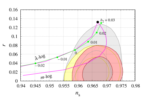
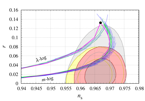
Figure 4: Spectral index $n_{s}$ and tensor-to-scalar ratio $r$ for $N=60$ in the case of the higher-order logarithmic corrections to the quartic coupling. The magenta, green, and blue lines represent the cases with corrections up to first, second, and third order, respectively. The black dot denotes the original quadratic chaotic inflation case. The Planck-allowed regions Planck are the same as in Fig. 1. Left: The case for $b_{2}=(-0.03)-0.03$ with $b_{1}=0.2$ and $b_{n}=0$ $(n\geq 3)$, as an example. The case of the first-order $m$-log correction is also shown. Right: All of the cases with both $\lambda$-log and $m$-log corrections explained in the text.

Let us now include the effects of the second-order corrections. We show the case for $b_{2}=(-0.02)-0.02$ with $b_{1}=-0.2$ as the green line in the left panel of Fig. 4. We observe that the second-order results are located near the (upper) magenta line. We also plot the cases for corrections up to the second and third order, respectively, as the green and blue lines (the upper branch) in the right panel of Fig. 4. We vary the parameter $b_{2}$ from $-0.02$ to $0.04$ for $b_{1}=(-0.3)-(-0.1)$ in the former case, while $b_{3}$ is set between $-0.005$ and $0.003$ for $b_{2}=(-0.02)-0.02$ and $b_{1}=-0.2$ in the latter case. Again, the resulting parameters $n_{s}$ and $r$ remain in a narrow region close to the (upper) magenta line where only the first order correction is included. We can thus deduce that the model with corrections of the form $\lambda(\log\phi^{2})\phi^{4}$ is only consistent with the Planck data alone, and may already be falsified by the combinations of the Planck, BICEP2/Keck Array, and/or BAO data. Therefore, we can distinguish the corrections to the mass from those to the quartic coupling, so that, in principle, it may reveal the form of the interactions of the model, when we obtain more precise CMB data in the future.

IV Conclusions

We have considered the logarithmic-corrected mass in the chaotic inflation model, and found that even this simple correction makes the model consistent with observations such as the CMB observation in Planck 2018, in combination with the BICEP2/Keck Array and baryon acoustic oscillation data. Since the model predicts a tensor-to-scalar ratio $r$ larger than 0.02 for the present allowed values of the spectral index $n_{s}$, the model will be tested in the near-future CMB polarization observations, such as those by the BICEP3/Keck Array BICEP3 and the POLARBEAR-2/Simons Array Simons .

In addition, we have considered higher-order logarithmic corrections, and found that $n_{s}$ and $r$ stay in a rather narrow region of the parameter space ($n_{s}$, $r$). Moreover, they reside in a completely different region from that for the logarithmic corrections to the quartic coupling as $\lambda(\log\phi^{2})\phi^{4}$. Therefore, future CMB polarization observations may figure out what the higher-order corrections would be, or even single out the form of the interactions.

References

- (1) A. D. Linde, Phys. Lett. 129B, 177 (1983).
- (2) Y. Akrami et al. [Planck Collaboration], arXiv:1807.06211 [astro-ph.CO].
- (3) V. N. Senoguz and Q. Shafi, Phys. Lett. B 668, 6 (2008).
- (4) K. Enqvist and M. Karciauskas, JCAP 1402, 034 (2014).
- (5) G. Ballesteros and C. Tamarit, JHEP 1602, 153 (2016).
- (6) K. Nakayama, F. Takahashi and T. T. Yanagida, Phys. Lett. B 725, 111 (2013).
- (7) K. Nakayama, F. Takahashi and T. T. Yanagida, JCAP 1308, 038 (2013).
- (8) K. Nakayama, F. Takahashi and T. T. Yanagida, Phys. Lett. B 737, 151 (2014).
- (9) F. Takahashi, Phys. Lett. B 693, 140 (2010).
- (10) K. Nakayama and F. Takahashi, JCAP 1011, 009 (2010).
- (11) K. Nakayama and F. Takahashi, JCAP 1011, 039 (2010).
- (12) S. Kasuya and F. Takahashi, Phys. Lett. B 736, 526 (2014).
- (13) R. Kallosh, A. Linde and D. Roest, Phys. Rev. Lett. 112, 011303 (2014).
- (14) C. Pallis, Phys. Rev. D 91, 123508 (2015) .
- (15) K. Kannike, G. Hütsi, L. Pizza, A. Racioppi, M. Raidal, A. Salvio and A. Strumia, JHEP 1505, 065 (2015).
- (16) L. Boubekeur, E. Giusarma, O. Mena and H. Ramírez, Phys. Rev. D 91 , 103004 (2015).
- (17) T. Tenkanen, JCAP 1712, no. 12, 001 (2017).
- (18) L. Järv, A. Racioppi and T. Tenkanen, Phys. Rev. D 97, 083513 (2018).
- (19) W. Buchmüller, E. Dudas, L. Heurtier, A. Westphal, C. Wieck and M. W. Winkler, JHEP 1504, 058 (2015).
- (20) K. Harigaya, M. Ibe, M. Kawasaki, and T. T. Yanagida, Phys. Lett. B 756, 113 (2016).
- (21) L. Marzola and A. Racioppi, JCAP 1610, no. 10, 010 (2016).
- (22) A. Racioppi, Phys. Rev. D 97, 123514 (2018).
- (23) M. Artymowski and A. Racioppi, JCAP 1704, no. 04, 007 (2017).
- (24) J. A. Grayson et al. [BICEP3 Collaboration], Proc. SPIE 9914, 99140S (2016).
- (25) N. Stebor et al., Proc. SPIE 9914, 99141H (2016).