Light-curve instabilities of $\beta$ Lyrae observed by the BRITE satellites

Abstract

Photometric instabilities of $\beta$ Lyr were observed in 2016 by two red-filter BRITE satellites over more than 10 revolutions of the binary, with $\sim$100-minute sampling. Analysis of the time series shows that flares or fading events take place typically 3 to 5 times per binary orbit. The amplitudes of the disturbances (relative to the mean light curve, in units of the maximum out-of-eclipse light-flux, f.u.) are characterized by a Gaussian distribution with $\sigma=0.0130\pm 0.0004$ f.u. Most of the disturbances appear to be random, with a tendency to remain for one or a few orbital revolutions, sometimes changing from brightening to fading or the reverse. Phases just preceding the center of the deeper eclipse showed the most scatter while phases around secondary eclipse were the quietest. This implies that the invisible companion is the most likely source of the instabilities. Wavelet transform analysis showed domination of the variability scales at phase intervals $0.05-0.3$ (0.65–4 d), with the shorter (longer) scales dominating in numbers (variability power) in this range. The series can be well described as a stochastic Gaussian process with the signal at short timescales showing a slightly stronger correlation than red noise. The signal de-correlation timescale $\tau=(0.068\pm 0.018)$ in phase or $(0.88\pm 0.23)$ d appears to follow the same dependence on the accretor mass as that observed for AGN and QSO masses 5–9 orders of magnitude larger than the $\beta$ Lyr torus-hidden component.

1 Introduction

$\beta$ Lyr (HD 174638, HR 7106) is a frequently observed, bright ($V_{\rm max}=3.4$ mag, $B-V=0.0$ mag) eclipsing binary. Hundreds of papers have been published about this complex system, which consists of a B6-8 II bright giant with a mass of about $3M_{\odot}$ and an invisible, much more massive companion ($\simeq 13M_{\odot}$) which occults the blue bright-giant every $P=12.915$ days producing primary (deeper) eclipses. The B-type bright giant loses mass to the more massive object at a rate which induces a fast period change, $dP/dt$ of 19 seconds per year; this period change has been followed and verified for almost a quarter of a millennium. The binary shares many features with the W Serpentis binaries which are characterized by the presence of highly excited ultraviolet spectral lines most likely energized by the dynamic mass-transfer between the components (Guinan, 1989; Plavec, 1989). The accretion phenomena related to the mass transfer from the visible component onto the more massive component lead to processes resulting in complex spectral-line variability, with the presence of strong emission lines (Harmanec et al., 1996; Ak et al., 2007), of X-ray emission (Ignace et al., 2008) and of variable spectral polarization (Lomax et al., 2012). The physical nature of the more massive component of $\beta$ Lyr remains a mystery, but it is normally assumed that it is a donut-shaped object with the outer regions completely obscuring the view of a central star expected to be roughly of B2 spectral type. The interferometric observations by the CHARA system confirm this general picture (Zhao et al., 2008). For further details, consult the review of the physical properties of $\beta$ Lyr by Harmanec (2002) which is a useful summary of what is known and what remains to be learned about the binary system.

Accretion phenomena in $\beta$ Lyr lead to light-curve instabilities. A dedicated international, multi-observatory campaign in 1959 (Larsson-Leander, 1969a, b) led to detection of instabilities as large as 0.1 mag. However, observational errors during this campaign were typically about 0.01 mag and temporal characteristics of the instabilities could not be firmly established. Because of the need for unifying data from many observatories, there remained a lingering possibility that the apparent light-curve instabilities could be at least partly explained by photometric calibration or filter-mismatch problems and by the presence of emission lines coupled to differences in photometric filters. All these problems were aggravated even further by the moderately long orbital period and by the diurnal interruptions. Although the 1959 photometric campaign left no doubt that the instabilities are present, their frequency and size remained poorly understood. In this situation, attempts to model the light curves (Wilson, 1974; Van Hamme at al., 1995; Linnell et al., 1998; Mennickent & Djurašević, 2013) were always confronted with a necessity to use orbital-phase averages with the assumption that the photometric instabilities are sufficiently random to permit such an averaging to obtain reliable mean light-curve values.

This paper sets as a goal characterization of the light-curve instabilities observed in $\beta$ Lyr by the BRITE Constellation (Weiss et al., 2014; Pablo et al., 2016; Popowicz et al., 2017) during 5 months in 2016 using the temporal sampling of the orbital periods of the satellites, i.e. 98 – 100 minutes. Section 2 describes the observations while Section 3 presents a mean light curve used in this paper as an auxiliary tool to derive photometric deviations from it. Section 4 discusses analyses of the light-curve instabilities treated as a time series using traditional tools such as the Fourier transform or autocorrelation function, and adding newer methods such as wavelets and recently developed methods to characterize variability of QSO and AGN objects. The concluding Section 5 summarizes the results.

2 BRITE observations

2.1 General description

The observational material obtained during the 2016 visibility season of $\beta$ Lyr consists mainly of photometric observations from two satellites of the BRITE Constellation equipped with red filters, “BRITE-Toronto” (BTr) and “Uni-BRITE” (UBr). The star was observed also by the blue-filter satellite, “BRITE-Lem” (BLb), but this satellite suffered from stabilization problems so that the observations covered less than one orbital period of the binary at the end of the BTr observations; as a result, the BLb data are not used in this paper.

The BRITE observations started on 4 May and ended on 3 October 2016 and thus lasted 152 days. The exposures were taken at 20-second intervals with the duration of 1 second for the UBr satellite, which is a typical choice for bright stars, preventing saturation of the CCD pixels. Unfortunately, UBr experienced stabilization problems for about a half of the $\beta$ Lyr run, so that most of the data were collected by the BTr satellite using 3-second exposures, which were more appropriate for $\beta$ Lyr. BTr was very well stabilized and provided excellent data in terms of their quality and quantity.

Figure 1: BRITE observations of $\beta$ Lyrae in 2016 versus time in $t=HJD-2\,456\,000$. The satellite-orbit averages (in magnitudes) shown in the figure resulted from standard pipeline and de-correlation processing. The orbital phases of the binary are given along the upper horizontal axis of the figure; they are counted continuously from the assumed zero epoch, as described in Section 2.4. The symbols and labels relate to different satellite “setups” as described in the text (BTr-2: triangles; BTr-3: crosses; BTr-4: filled circles; BTr-5: slanted crosses; UBr: open circles). While the magnitude system is arbitrary, the amplitude of the BTr variability is larger compared with that observed by UBr; note the light-curve shape defined by the small, filled circles and by the overlapping larger, open circles. This unexpected result led to the discovery of an instrumental problem which is described in Section 2.2. All available red-filter observations are shown here including those which were not used in the detailed analysis limited to the BTr-3, BTr-4 and UBr setups. The blue-filter BLb observations, which are not shown, took place at the end of the BTr-4 run, at $1637<t<1647$ and covered about 0.7 of the binary orbital period.

The distribution of the BRITE magnitudes versus time is shown in Figure 1. Since the BRITE data are used mainly for studies of stellar variability, the zero point of the magnitude scale is arbitrary and is adjusted for each of the “setups” marked by labels in the figure. A “setup” is a set of positioning instructions for the satellite and for the CCD windowing system, as described in full in the Appendix to Popowicz et al. (2017). Occasional changes of setups result from addition or removal of stars from the observed field without changes of the remaining star positions, while some changes are necessary because of satellite stability issues or Earth-shine scattering problems. The concept of the “setup” is important, as it divides the data into series which may show small magnitude shifts. The division into setups continues through the initial raw-data processing so that each setup can be identified as leading to a separate time series. Several setups were inadequate for the current investigation: The first BTr setup could not be used because of imperfections in the initial positioning, the BTr-2 was shorter than one orbital period of $\beta$ Lyr, while the data for the last setup BTr-5 showed strong signatures of being affected by scattered sunlight at the end of the season. In the end, this paper utilizes the data for the setups BTr-3, BTr-4 and the combined data for the setups UBr-1 and UBr-2 (from now on, UBr). The ranges in time and the numbers of observations in each setup are listed in Table 1.

2.2 Discovery of an instrumental problem

The data processing followed the routine steps described in Pablo et al. (2016) and Popowicz et al. (2017) with subsequent de-correlation as described by Pigulski (2018). Even a cursory comparison of the raw data (Figure 1) reveals a large difference in the amplitude of $\beta$ Lyr as measured by UBr and BTr, with BTr observing amplitudes larger than one magnitude, a value never encountered before. It was obvious that a previously unrecognized problem affected the BTr observations. It went undetected because none of the previously observed variables had such a large and well known amplitude. Detailed comparison of the resulting light-curve shapes and lack of any indications for photometric non-linearity in the system led us to consider a linear transformation of the detected signal involving a loss of detector charge, somewhat similar to a locally different CCD bias. Further investigation revealed shallow spots in the CCD response where electrons were trapped by charge-transfer-inefficiency (CTI) effects, apparently due to radiation damage. This problem was reported before in a note about the same BRITE observations (Rucinski et al., 2018). Unfortunately, there were no contemporary data on the spots for the time of the $\beta$ Lyr run, but from archival data it was estimated that in April 2015 – when an edge part of a blank field was affected by scattered sunlight – the depressions covered about 2.5 to 4 percent of the BTr detector area. The new data taken in July 2017 indicate that the amount of the affected area has grown in time as a result of progressing detector damage. Discovery of the problem by our observations has opened up a full investigation which is currently ongoing. In addition to the note by Rucinski et al. (2018), the problem has been discussed with other instrumental issues affecting the BRITE satellites by Pigulski et al. (2018) and Popowicz (2018).

The problem was detected mostly thanks to the large and well-known amplitude of $\beta$ Lyr; it has minimally affected most of the previous studies concentrated on small-scale pulsational variabilities. In fact, since this paper is devoted to deviations from the smooth light curves, we could ignore this new CTI effect and use the otherwise excellent BTr data without any correction. Such results would be spoiled by a scale problem, though, and the mean light curve would be entirely invalid. Fortunately, it was possible to correct the BTr data by using the partially simultaneous data from the UBr satellite. In doing this correction, we assumed that the UBr signal was not systematically modified in any way and that the proper BTr signal can be restored by a simple linear transformation relating the CCD charges (or light fluxes) $f_{\rm UBr}$ and $f_{\rm BTr}$: $f_{\rm UBr}=a_{0}+a_{1}f_{\rm BTr}$. Here, $a_{0}$ and $a_{1}$ are constants to be determined by least-squares fits, with $a_{0}/a_{1}$ representing the lost charge expressed relative to the maximum signal for $\beta$ Lyr as observed by UBr ($f_{\rm UBr}$ was normalized to unity at the binary light maxima). The temporal constancy of the problem is obviously an assumption, but it seems to be a plausible one in view of (1) the stability of the final results and (2) the most likely cause of the CTI damage as due to infrequent local damage of the CCD lattice caused by very energetic radiation particles. The fluxes were determined by the standard flux-magnitude relation, $f=10^{-0.4(m-m_{0})}$, assuming the maximum light ($m_{0}$) magnitudes for the setups: $m_{0}({\rm UBr})=3.81$, $m_{0}({\rm BTr2})=m_{0}({\rm BTr3})=3.54$, and $m_{0}({\rm BTr4})=3.59$, where the magnitudes are those resulting from the standard BRITE pipeline and de-correlation processing. The transformation linking the UBr and BTr-4 data was possible for 50.14 days (or 3.87 $\beta$ Lyr orbital periods) of simultaneous observations of the two setup sequences. Thanks to the very high number of overlapping observations of the UBr run (16,686), the transformation relating the $f_{\rm UBr}$ and the $f_{\rm BTr}$ fluxes was very well determined: $a_{0}=0.20392\pm 0.00046$, $a_{1}=0.79688\pm 0.00063$, with the amount of the signal lost, in terms of the maximum $\beta$ Lyr signal: $a_{0}/a_{1}=0.25589\pm 0.00077$. The errors here were determined by 10,000 bootstrap repeated solutions. No systematic temporal trend was detected in the transformation.

2.3 Satellite-orbit average data

Observations of $\beta$ Lyr by both satellites experienced breaks due to Earth eclipses which naturally divided the individual observations into groups separated by gaps when the field was either invisible due to Earth occultations or strongly affected by the Earthshine. The median number of individual observations in the groups was 40 for BTr and 37 for UBr. Thus, with 3 observations per minute, the uninterrupted observations lasted typically 12 – 13 minutes. However, some groups were as long as 75 continuously acquired observations and some as short as 8 observations, so that the averaged data have different errors: For BTr, the errors range between 0.0005 and 0.0045 with the median error (assumed to be typical) 0.0014; for UBr, the errors range between 0.0004 and 0.0058 with the median error 0.0019, all expressed in flux units (f.u.) relative to the maximum $\beta$ Lyr flux. The better quality of the BTr data is a result of the longer individual exposures of 3 sec, compared with 1 sec for UBr.

The satellite orbital periods at the time of the $\beta$ Lyr observations were: 0.06824 d = 98.3 min for BTr and 0.06974 d = 100.4 min for UBr. Expressed in units of the binary-star period, the satellite-caused spacing in $\beta$ Lyr orbital phase was 0.005273 for BTr and 0.005388 for UBr, or 190 and 186 group averages per one orbital period of the binary, setting respective upper limits on frequencies of detectable instabilities. The satellite-orbit average fluxes of $\beta$ Lyr are given in Table 2. The table lists the mean time, the orbital phase as in Section 2.4, the average flux with its error, and the number of observations per average.

2.4 The orbital-phases of $\beta$ Lyr

The orbital period of $\beta$ Lyr has been studied by many investigators. It is now well established that the period change rate is very close to being constant and that a parabolic $O-C$ diagram for the times of minima very well describes the expected moments of eclipse minima. We used the elements of Ak et al. (2007) to set a locally linear system of phases for the epoch $E=3811$: $\phi=(t-1518.6251)/P$, with $P=12.943296$ corrected for the $dP/dt$ change and $t$ as defined in Section 2.1.

From now on in this paper, we will use the term “orbital phase” or just “phase” as the main independent variable versus which the physical variability of $\beta$ Lyr is taking place. The phase is counted as a number including the integer part, as shown along the upper horizontal axis of Figure 1. Traditionally, the meaning of the term “phase” is a number confined to the interval 0 to 1; such a use as a fractional phase appears sparingly in this paper. The phases of our observations cover the range from about zero for the (not used) setup BTr-2 data to about eleven at the end of the (also not used) setup BTr-5. The two BTr setups which were utilized cover the phase ranges $0.11<\phi<2.66$ and $2.66<\phi<10.30$ for BTr-3 and BTr-4, respectively. This system of local phases is used in the paper as an independent variable in place of the time in our discussion of the photometric instabilities treated as a time series (Section 4).

Figure 2: The mean light curve of $\beta$ Lyrae obtained by averaging satellite-orbit means for the setups BTr-3 and BTr-4 in intervals of 0.01 in fractional orbital phase. The light curve is expressed in relative flux units (f.u.) with the maximum light assumed as unity. The error bars are comparable to or smaller than the symbols used for the light curve (the upper panel). The errors with their uncertainties, estimated from the number of points per phase interval, are shown separately in the middle panel. The lowest panel gives the light-curve derivative in f.u. per 0.01 phase interval with uncertainties estimated from the errors of adjacent flux values. The vertical lines give the phases of external eclipse contacts (at $\pm 0.114$ relative to the eclipse centers), calculated using the unpublished model by Pavlovski et al. (2018).

3 The mean light curve

The mean light curve for $\beta$ Lyr has been formed from the combined observations of the BTr-3 and BTr-4 setups. The curve itself is not used in this work except for removal of the global eclipsing variations and thus to determine the light-curve instabilities. The mean light curve is very well defined (Figure 2); it has been obtained by averaging the individual, satellite-orbit, average data points in 0.01 intervals of binary fractional orbital phase. Typically (median) 16 points per phase interval contributed to a single point, with the actual numbers ranging between 12 and 20 for individual satellite-orbit mean points. The flux error per average point ($\sigma_{\rm mean}\simeq 0.0042$ f.u., $\sigma_{\rm median}\simeq 0.0036$ f.u.) is dominated by the $\beta$ Lyr light-curve instabilities which we discuss in the rest of this paper. The errors show an increase during the eclipse branches as expected when the data are averaged on slopes and consequently correlate with the absolute value of the derivative (the lowest panel in Figure 2). Judging by the size of $\sigma_{\rm median}$ and the number of observations per interval, typical deviations of the instabilities are expected to show a scatter with $\sigma_{\rm dev}\simeq 0.014$, a number which is confirmed by a more detailed analysis in Section 4. This is in fact a smaller number than was originally expected for the combined BTr-3/BTr-4 observations lasting as long as four months. Unless we observed $\beta$ Lyr in a particularly inactive time, this may indicate that the previous indications of large photometric instabilities reaching 0.1 mag were partly affected by inconsistencies in filter-matching and by other data-gathering and collation steps.

The excellent definition of the BTr light curve permitted determination of its derivative $df/d\phi$, as shown in Figure 2. In addition to the expected large absolute values within the eclipses, the derivative reveals some structure beyond the eclipses which may indicate phenomena not accounted for by the standard stellar-eclipse model.

A phase-shift apparently caused by a small asymmetry appears to be present for the primary (deeper) minimum for the time-of-eclipse elements of Ak et al. (2007). The shift is estimated at $+0.0076\pm 0.0002$ in phase, corresponding to $+0.0984\pm 0.0026$ day or $+2.36\pm 0.06$ hours. No significant shift, at the same level of uncertainty as for the primary, was noted for the secondary eclipse. The presence of the primary-eclipse phase shift may be related to the 283 day periodicity in the times of the primary eclipses which was noted before (Guinan, 1989; Kreiner et al., 1999; Wilson & Van Hamme, 1999; Harmanec, 2002) and which still does not have an explanation (Section 4.2). Since the secondary minimum did not show any shift, the phase system of Ak et al. (2007) was adopted for our investigation without any modification.

In addition to the BTr mean light curve, an independent light curve was formed from the UBr observations. It is not equally well defined because larger gaps in the $\beta$ Lyr phase coverage resulted in only 92 points for the same, 0.01-wide phase interval. Consequently, the deviations for the UBr series, used later to fill in gaps in the BTr satellite data, were defined in reference to the BTr mean light curve. The UBr and BTr fluxes are expected to be in the same system through the transformation described in Section 2.2.

Figure 3: The light-curve deviations $\delta$ from the mean as a function of the orbital phase of $\beta$ Lyr. The deviations used in the analysis are for three setups: BTr-3 (upper panel), BTr-4 (middle) and UBr (lower panel). The BTr-3 series precedes the BTr-4 while that for UBr is aligned to show the same orbital phases as for BTr-4. The deviations $\delta$ are expressed in flux units. The mostly positive values of the deviations for the BTr-3 series and slightly negative ones for the BTr-4 series result from the use of the combined BTr-3 and BTr-4 data for formation of the mean light curve. The wavy, broken-line curve in the BTr-4 panel gives the low-frequency approximation by a 5th-order Chebyshev polynomial, as discussed in Section 4.2. The three largest gaps in the uniform, equal-step BTr-4 coverage which could not be filled by the UBr observations were interpolated over 7, 12 and 7 equal-step intervals; they are marked by short bars along the upper axis of the figure (phases: 4.22–4.25, 6.10–6.16, 9.85–9.89).

4 The light-curve instabilities

4.1 The $\delta$-deviations as a time series

We used deviations of the individual satellite-orbit averages from the mean light curve to characterize the light-curve instabilities. The deviations, $\delta$, are shown versus $\beta$ Lyr orbital phase in Figure 3. The data are continuous for the adjacent BTr-3 and BTr-4 setups, while those provided by UBr overlap over a part of the BTr-4 series. For the BTr observations, the temporal (satellite orbit) sampling was 98.3 minutes, while for UBr the sampling was 100.4 minutes, with average deviations from uniform sampling of $\pm 2.4$ minutes for BTr and $\pm 1.5$ minutes for UBr. The BTr-3 and BTr-4 series are of different lengths, covering together the $\beta$ Lyr phases for 10 orbital cycles ($0.11<\phi<10.30$). For the final application, the BTr-4 series was shortened to end at $\phi=9.95$ to avoid the poorly covered observing time when the satellite-viewing field was getting into the Sun-illuminated part of the sky. Descriptions of the individual series are given in Table 4.

After careful consideration of the individual time series, we decided to use only the BTr-4 data for a study of the light-curve instabilities. The series BTr-3 is short and shows a trend with an unexplained jump by $\delta\simeq+0.045$ close to $\phi=0.9$ (it is probably significant that the jump coincides in fractional phase with phases of increased activity in the BTr-4 series, see below in Section 4.3). The UBr series has poor phase coverage with larger errors of individual data points, but it was useful to fill gaps in the BTr-4 coverage. It should be noted that the series BTr-3 and BTr-4 appear to have been correctly adjusted in terms of the magnitude shift during the initial processing stage since the $\delta$ deviations appear to be continuous (and fortuitously close to zero) at the transition point at $\phi=2.7$ (Figure 3).

The BTr-4 series extending into the orbital phase interval $\phi=2.661-9.948$ and sampled at satellite-orbit intervals with the mean $\Delta\phi=0.0052726$ can be subject to time-series analysis. To form a perfect equal-step sequence, we used $\Delta\phi$ as the main unit of the equal-step grid. Such a series of 1383 equidistant points had gaps as 1222 satellite averages were actually observed. Since the UBr and BTr flux scales are identical through the scaling operation, as described in Section 2.2, we were able to fill the gaps using the UBr data. Except for an unexplained spike observed at $\phi\simeq 7.25$, when UBr was returning to normal operations after an instrumental interruption, the UBr and BTr data agree very well (Figure 3). Fortunately, there was no need to use the spike phases for filling the BTr-4 series, while the UBr data filled very well the BTr gaps at phases $\phi\simeq 5.7$ and 7.8. We used UBr observations with a restriction that they could be spaced no more than one satellite orbit away from the missing interval for interpolation into the BTr-4 series. The addition of 77 points increased the number of observed points to 1299 and the final coverage efficiency to 93.9 percent. The remaining gaps were spline-interpolated within the filled series, typically over one to three missing points. The three larger gaps, one of 12 and two of 7 intervals do not seem to affect the shape of the series in an obvious way; they are marked in Figure 3 as short bars along the upper axis of the BTr-4 panel.

4.2 The 283 day periodicity and its implications

In addition to apparently random perturbations, the light curve of $\beta$ Lyr is known to show a possibly periodic variation beyond that of the binary orbit, which has so far eluded explanation. It was detected in the deviations from the mean light curve by Guinan (1989) who estimated their period at $275\pm 25$ days. Later, using archival data, Van Hamme at al. (1995) found the period of 283.4 days, while Harmanec et al. (1996) found 282.4 days, with similar uncertainties of about $\pm 0.1$ day. The maximum semi-amplitude estimated from these analyses was about 0.03 of the mean flux. The period of 283 days was later confirmed by Kreiner et al. (1999).

While the analyses by Van Hamme at al. (1995) and by Harmanec et al. (1996) showed agreement in the description of the archival material, the uncertainty in the period precludes forward prediction reaching the epoch of our observations. With the duration of 3 months, the BRITE observations did not last long enough to address the 283 day periodicity directly, however, we could look for shorter, possibly related time scales. In particular, Harmanec et al. (1996) discussed a possibility that the 283 day periodicity results from beating of the orbital period with variability at 4.7 – 4.75 days estimated for the emission lines emitted by a precessing jet from the accreting component.

Our $\delta$-series does show a slow, wavy trend extending over the whole duration of the run (Figure 3). However, since the data were affected by the problem with the missing CCD charges (Section 2.2), our initial reaction was to treat the slow trend as having an instrumental explanation and to remove it. Such removal would obviously force the analysis to address only the short time-scales, comparable to or shorter than the $\beta$ Lyr period. The slow trend was removed by utilizing the excellent approximation properties of the Chebyshev-polynomials: The $\delta$-series was converted into a series of such polynomials, all their coefficients for orders $>\!5$ were set to zero and then the series was re-converted back to the time series. The resulting low-frequency wave with the range $-0.0132$ to $+0.0104$ f.u. was subtracted from the observed deviations to form a “trend-subtracted” series.

After the analysis of the trend-corrected data using tools developed for AGN and QSO light-curve instabilities (Section 4.6) we realized that the uncorrected data present a more consistent picture of a Damped Random Walk (DRW) process. For that reason, we carried out the analysis for both the uncorrected (mean-subtracted) and the trend-corrected series of deviations (Table 5) and attempted to monitor the resulting differences. The deviations of both series follow a Gaussian distribution with largest deviations reaching $\pm 0.04$ f.u. for the uncorrected series. As expected, the standard deviation for the uncorrected series is larger: $\sigma=0.0130\pm 0.0004$ f.u. while it is $\sigma=0.0109\pm 0.0003$ f.u. for the trend-corrected series. The distributions of the deviations are shown in an insert in Figure 4. The remaining parameters of the Gaussian fits are: The maximum value $N_{\rm max}=84.8\pm 2.3$ and $99.6\pm 2.4$; the zero-point shift $\delta_{0}=+0.0006\pm 0.0004$ f.u. and $+0.0011\pm 0.0003$ f.u., respectively for the uncorrected and the trend-corrected data. We recall that the median error of the individual data point of the series was estimated at $\sigma=0.0014$ f.u.

Figure 4: The auto-correlation function (ACF) for the $\delta$ series. The horizontal axis gives the correlation lag in units of the $\beta$ Lyr orbital period. The dotted line gives the ACF for the trend-corrected series, as explained in Section 4.2. The dashed line close to the origin shows the model ACF (Equation 1) obtained by an independent analysis of the Structure Function (SF) for the series treated as a Damped Random Walk process using Equation 4, with $SF_{\infty}=0.0179$ and $\sigma_{n}=0.0014$; see Section 4.6. The insert gives the histogram of the versions of the $\delta$ series, with a Gaussian fit (continuous line) for the series as observed, without the trend correction.

4.3 The frequency content

The brightening and fading events in the light curve – relative to its mean level – appear as up- and down-directed spikes in the $\delta$ series. They tend to occur at time scales shorter than one orbital period of $\beta$ Lyr, typically within $0.1P$ to $0.3P$ (Figure 3). We counted 27 brightening and 25 fading events during the seven fully observed cycles of the series, giving the corresponding rates $4.0\pm 0.8$ and $3.6\pm 0.7$ of such events per orbital period of $\beta$ Lyr. This is exactly the domain of temporal fluctuations most difficult to characterize using ground-based data for the orbital period of $\beta$ Lyr. Although scales shorter than one orbital period seem to dominate, we note that variability has components which include small multiples of the binary orbital period. Activity at a given phase may take the form of either a decrease or increase in brightness. For example, a series of brightening events took place just before $\phi=4-6$, while a more conspicuous dip repeated just before the very center of the primary eclipse, at $\phi=7-9$ (the approximate visual estimates gave spikes occurring at phases 2.93, 3.95:, 4.93:, while dips were at 5.92:, 6.96, 7.96, 8.96, 9.96:; the colon signifies a larger uncertainty).

We used the Auto-Correlation Function (ACF) and the Fourier Transform in its Fast (FFT) and Discrete (DFT) realizations for the presence of coherent variability in the $\delta$-series. The orbital phase of $\beta$ Lyr served as the time variable without a correction for the progressing orbital period change of 5 seconds which took place within the span of our observations (Section 2.4). We considered this effect as unimportant due to the moderate duration of the run (7 orbital cycles or 1/4 year, in view of the period change of 19 seconds per year), and the data sampling of one point every 98.3 minutes.

The ACF of the $\delta$-series in Figure 4 shows positive correlation at the delay of one orbital period, $P$, and then consecutive negative spikes at multiples of $P$, starting from the delay of $3\times P$. Thus, whatever pattern emerges in the deviations, it tends to last for no more than one orbital period, but is likely to re-appear after a delay of more than two orbital periods in the form of an opposite deviation. Obviously, the limited length of the time series makes the results for lags larger than about a half of the length of the data series very uncertain.

Figure 5: The Discrete Fourier Transform for the the $\delta$-series, expressed as cycles per orbital period of $\beta$ Lyr (c/orb). The short dashes within the figure mark integer values of the orbital frequency. The vertical axis of the figure gives the amplitude of oscillations in flux units relative to the maximum light of the binary. The results shown by the dotted line correspond to the trend-corrected version of the series.

The FFT and DFT transforms of the $\delta$-series gave identical results. Figure 5 shows the low-frequency end of the DFT ($f<12$ c/orb). With the sampling of 98.3 minutes ($0.0052726\,P$) there are 189.6 data points per orbital period of $\beta$ Lyr leading to the nominal resolution of 0.1372 c/orb.

The uncorrected and the trend-corrected versions of the series give practically identical results for frequencies above one cycle per binary orbit, where well-defined, coherent variability components with frequencies corresponding to one and two cycles per period $P$ are easily detectable in the data. Several higher multiples are also present, but they decrease in size for higher frequencies and appear to be entirely absent for $f>\!12$ c/orb. As expected, the low frequency content is very different in the two versions of the series with a very strong drop in amplitudes for $f<1$ c/orb for the trend-corrected series; there are no detectable components for $f<0.3$ c/orb. The strongest frequency in the trend-corrected series is located close to 2 c/orb ($1.90\pm 0.13$ c/orb) and is due to the two similar eclipses during one orbital period. Its amplitude is 0.0058 f.u. which is only 3.5 times larger than the median data error. Its removal from the FFT and re-transformation back to the time series does not change the series in an obvious way leaving the general random appearance of the series practically unchanged. For the uncorrected series, the largest peak in the transform is located at 0.240 c/orb, with the amplitude of 0.0077 f.u.

An estimate of errors in the FFT/DFT transforms is used for normalization of the results of the wavelet analysis in Section 4.5. The assumed error of the white-noise power was estimated from high frequencies of the transform, $f>\!60$ c/orb, at $\sigma_{\rm FFT}\simeq 1.5\times 10^{-4}$ f.u. This estimate is about 4 times larger than the expected value using the median of the individual errors, $\sigma=0.0014$: $\sigma_{\rm FFT}=\sigma/\sqrt{(}1383)=3.8\times 10^{-5}$ f.u., reflecting the presence of individual, much poorer measurements in the series (Section 2.3); however, a contribution of very rapid variability is also not excluded.

Figure 6: The deviations of the $\delta$-series without the trend correction, fitted by the scaled version of the $\beta$ Lyr mean light curve in intervals of full orbital cycles. The gaps in the BTr coverage, filled by the UBr data are marked by open circles.

Figure 7: The $\delta$ deviations of the uncorrected series are shown versus the fractional phase of the $\beta$ Lyr orbit. The lower panel gives the standard deviation $\sigma$ computed using Gaussian-distribution fits to the deviations in 0.1-wide phase intervals.

4.4 The binary-phase dependence

Since the orbital period of $\beta$ Lyr together with its harmonics leaves an imprint in the $\delta$-series, an attempt was made to fit the scaled light curve of the binary to individual segments of the series. This would verify if the deviations are perhaps simply reflections of the light-curve shape projecting into the series. An assumption was made of the exact phase coherence of the $\delta$-deviations with the $\beta$ Lyr light curve over each separate orbit interval. Obviously, this is highly simplistic as disturbances may emerge or disappear at any orbital phase and do not have to last exactly one orbital period. No other assumption was made, i.e. the light-curve imprint into the deviations could be either positive or negative corresponding to flares or fading dips. The fits are shown in Figure 6. In most cases, the fits are inadequate, with the only exception at cycles $\phi=7-8$ where the deviations do mimic the light curve. There is no agreement for earlier cycles, with an inverted dependence for the cycle $\phi=3-4$ and no dependence in cycles $\phi=4-5$ and $9-10$. Thus, we do see a certain persistence of the disturbances with the orbital period of the binary, but generally the correlation with the light curve is poor.

An inspection of Figure 6 suggests that large, positive and negative deviations tend to occur at phases just preceding the center of the primary eclipse when the B6-8 II star is eclipsed by the torus around the more massive component. The distribution of deviations binned into the fractional phase intervals of the $\beta$ Lyr orbit, as in Figure 7, shows the largest spread in the deviations in the orbital phases around 0.9 – 1.0. There, the individual deviations reach $\pm 0.05$ leading to $\sigma=0.027$, which is almost twice what was observed at phases of the secondary eclipse when the more massive component is eclipsed. Thus, our observations point at the region close to the central parts of the torus around the more massive component as the location of the photometric disturbances, although it is of course impossible to tell if this is a permanent feature or a tendency which just occurred during the BRITE observations.

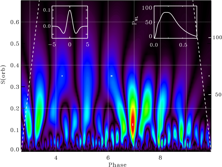
Figure 8: Wavelet analysis of the $\delta$ series, the version with the low frequency trend removed (see the text). The horizontal axis is the orbital phase of $\beta$ Lyr, the same as in previous figures. The vertical axis is the horizontal scale $S$ of the wavelet analyzing function – in this case the DOG-2 or “Mexican hat” function – expressed in units of the orbital period, $P$; the right vertical axis gives the scale in numbers of the data points of the series. The broken lines delineate areas affected by edge effects. Short horizontal bars in the middle of the picture give phases of points which were not observed and later interpolated in the equal-step series; they do not seem to exhibit any detrimental effects on the results. The left insert gives the shape of the DOG-2 function; the horizontal scale is in units of the data-point spacing while the vertical axis has been normalized to give the integral of one. The right insert shows the variability power relative to the white noise of the series with the horizontal scale in units of the orbital period of the binary and the vertical axis giving the variability power normalized by the white-noise power, $p_{\rm FFT}$ (see text).

4.5 Wavelet analysis

Wavelet transforms permit characterization of the variability in terms of time-scales and of locations of disturbances in the time series. In using wavelets, we followed the formulation of Torrence & Compo (1998), where the literature of the subject and useful recommendations are given. Three types of wavelets, Morlet-6, Paul-4 and DOG-2, were used to perform the continuous wavelet transforms of the $\delta$ series: The Morlet-6 wavelet detects localized sinusoidal wave packets, while Paul-4 and DOG-2 are sensitive to localized groups of deviations for which the time-scale characterizes the duration of the event. The numerical descriptors in the wavelet names provide additional information about the type of the analyzing function, e.g. for Morlet-6 the Gaussian-bound wave packet contains 6 oscillations, while DOG-2 is an abbreviation for the second derivative of the Gaussian (this function is also known as the “Mexican hat” wavelet).

Although the Morlet-6 transform has been known to function very well for detection and frequency characterization of localized and/or evolving wave trains, it did not lead to a detection of such periodic events in the $\delta$ series. We found that both Paul-4 and DOG-2 performed similarly for characterization of the spiky disturbances in the series. Since the Paul-4 transform, when expressed as the variability power (or square of the amplitude) and interpreted in terms of the size and time-scale gave very similar results to the more popular DOG-2 wavelet, we describe here the results only for the latter transform. We analyzed both of the $\delta$ series, with and without the low-frequency trend removed. The uncorrected version was very strongly dominated by time scales longer than about $0.5\,P$ due to the large content of variability power at low frequencies, at time scales $\gg\!P$. This forced us to consider only the trend-corrected series, recognizing that this will give information only about shorter time scales.

A wavelet transform unfolds the one-dimensional time series into a 2-D picture where the abscissa is the time (or in our case the full $\beta$ Lyr orbital phase), while the ordinate is the scale of the disturbance, $S$, as shown in Figure 8. The scale corresponds to the expansion or stretching of the assumed wavelet function, in our case the DOG-2. As discussed in Torrence & Compo (1998), the scales can be related to the frequencies in the FFT picture; it is also possible to link the FFT oscillations power to the wavelet-estimated power of the disturbances, irrespectively of their shape, as long as the analyzing wavelet function obeys a certain number of conditions. For the figure, we used the wavelet power normalized to the white-noise power estimated from the FFT transform, $\sigma_{\rm FFT}\simeq 1.5\times 10^{-4}$ f.u. (Section 4.3), following the recommendations of Torrence & Compo (1998).

The variability power over the duration of the run, $p_{\rm WL}$, is the sum of the wavelet components for the same scales $S$, as projected into the vertical axis of Figure 8 (the right insert). We see that although most disturbances appear with short time scales of $0.05P-0.1P$ (or 10 – 20 data points), in terms of the variability power, the maximum is located at scales of $0.2P-0.3P$ (or 40 – 55 data points); this may signify dominance of the largest brightening and dimming events in the power budget. The broad range $0.05P-0.3P$ corresponds to time scales between 0.65 day and 4 days, i.e. exactly in the domain of variability which is particularly difficult to study from the ground for $\beta$ Lyr because of diurnal interruptions.

4.6 Modeling $\delta$-series as a stochastic process

The light-curve instabilities in $\beta$ Lyr are most likely caused by the ongoing mass transfer process and may reflect changes in the accretion rate onto the hidden, more massive component. Accretion is recognized as the key process in active galactic nuclei (AGNs), where it is responsible for both typically huge AGN luminosity and its significant ($\sim$10%) random variability. The recent years have seen development of modern statistical tools specifically targeting such aperiodic variations. The damped random walk (DRW) model (Kelly et al., 2009) is particularly powerful as it describes the variable signal using only two parameters: (1) the signal de-correlation time scale $\tau$ and (2) the modified amplitude of the stochastic signal $\hat{\sigma}$ or, equivalently, $SF_{\infty}$ (Kozłowski et al. 2010; MacLeod et al. 2010; Zu et al. 2013).

In the DRW model, the variable signal is correlated for frequencies $\nu$ higher than $\tau^{-1}$ and resembles red noise (the higher the frequency, the stronger the correlation), with power spectral density $PSD(\nu)\propto\nu^{-2}$, while for frequencies lower than $\tau^{-1}$ it becomes white noise ($PSD(\nu)\propto\nu^{0}={\rm const}$). Conformity of the time series with the DRW model can be tested by the PSD analysis or the structure function (SF) analysis that have one additional model parameter, the power-law slope of the correlated noise (e.g., Simonetti et al. 1984; Kozłowski 2016a). When analyzed using the SF, which is a measure of the variability amplitude as a function of the time difference between points, the DRW process is expected to show a power-law slope ($\gamma=0.5$) for time scales shorter than $\tau$, flattening to $\gamma=0$ at time scales longer than $\tau$. The signal de-correlation time scale $\tau$ has exactly the same meaning in all the three methods: DRW, PSD and SF, so that consistent results for $\tau$ give an additional verification of the model. The second parameter of the DRW, the modified amplitude of the stochastic process $\hat{\sigma}$, is related to $\sigma_{\infty}$ as $\sigma_{\infty}=\hat{\sigma}\sqrt{\tau/2}$. The data separated in time by more than $\tau$ show variability best described by the white-noise statistics; $\sigma_{\infty}$ is the amplitude of the white noise, while $SF_{\infty}$ is the SF amplitude at long time scales, where $SF_{\infty}=\sqrt{2}\,\sigma_{\infty}$. All three methods are also interconnected by the auto-correlation function (ACF) of the signal, which we generalize here as the power exponential (PE; e.g., Zu et al. 2013)

$${\rm ACF}(\Delta t,\tau,\beta)=e^{-(|\Delta t|/\tau)^{\beta}},$$ (1)

where $0<\beta<2$, $\beta=1$ corresponds to DRW, and $\Delta t$ is the time difference between points. The conversions between the correlated part of PSD, described as the power-law with the slope $\alpha$, the structure function (the slope $\gamma$) and the PE (the slope $\beta$) are:

$$\alpha=-(\beta+1),$$ (2)

and since the SF slope $\gamma=\beta/2$, we have:

$$\alpha=-(2\gamma+1),$$ (3)

(e.g., Bauer et al. 2009; Kozłowski 2017c).

Figure 9: The SF analysis of the $\delta$ series, where the filled circles are for the original data while the open circles are for the trend-subtracted version of the series. The values of SF have been calculated with the IQR method, while the solid line is the best-fit, four parameter SF model to the filled dots. The de-correlation timescale $\tau$ is marked by an arrow. The shallow dips at $\Delta t=1.0P$ and $4P$ correspond to an increased correlation, that most likely originates from what can be readily seen as repeating dips in the $\delta$ series around the fractional phase 0.95, as shown in Fig. 6. The dotted line is the ACF from Section 4.3 converted to SF using Equation 4 with $SF_{\infty}=0.0179$ f.u. and $\sigma_{n}=0.0014$ f.u.

The SF for the $\delta$-series (Figure 9) was calculated using the inter-quartile range (IQR) method (introduced by MacLeod et al. 2012; see Eqns. (10) and (20) in Kozłowski 2016a). We model it as a four-parameter function as in Kozłowski (2016a):

$$SF^{2}(\Delta t)=SF_{\infty}^{2}\left(1-{\rm ACF}(\Delta t,\tau,\beta)\right)+2\sigma_{n}^{2},$$ (4)

where the parameters of interest are: $\tau$, $\beta$, $SF_{\infty}$, and the photometric noise $\sigma_{n}$. The best-fit parameters are: $SF_{\infty}=0.0179\pm 0.0003$ f.u., $\beta=1.19\pm 0.17$, $\tau=(0.068\pm 0.009)P$, $\sigma_{n}=0.0014$ f.u. (fixed), and the reduced $\chi^{2}=1.00$. These parameters correspond to: $\sigma_{\infty}=0.0127\pm 0.0002$ f.u., the SF slope $\gamma=0.60\pm 0.08$, the PSD slope $\alpha=-2.19\pm 0.17$.

We observe two shallow dips in the flat part of SF at $1P$ and $4P$, pointing to a periodic signature in the SF (see below), otherwise the $\delta$-time series is fully consistent with a stochastic-process realization. With the length of $7P$, the $\delta$-series is much longer than the de-correlation timescale ($>$$100$). This enables the usage of an alternative method to measure the de-correlation time scale from SF introduced recently by Kozłowski (2017b): we find $\tau=0.066_{-0.027}^{+0.023}$ $P$ which is consistent with the result above.

Since the $\delta$-series is much longer than $\tau$, it is possible to reliably estimate the DRW parameters (see Kozłowski (2017a) for a discussion of DRW biases and problems), although the “red noise” part appears to be slightly steeper ($\gamma=0.60$) than that expected for the DRW ($\gamma=0.5$). The different slope is expected to lead to biased parameters (Kozłowski 2016b), with the resulting $\tau$ longer than the true value by about $\sim$40%. We modeled the $\delta$-light curve with the DRW model presented in Kozłowski et al. (2010). The best-fit parameters are: $\tau=0.092_{-0.014}^{+0.021}P$ and $\sigma_{\infty}=0.0136\pm 0.004$. As expected, because the signal has a stronger correlation than the red noise, the de-correlation time scale turned out to be longer than the measurement obtained using the SF. We present the best DRW model describing the $\delta$-series in Fig. 10. In addition to the methods described above, we modeled the PSD in the least-squares sense, as described before for the DRW function (Eq. (2) in Kozłowski et al. 2010), and obtained $\tau=(0.065\pm 0.014)P$, again consistent with the above estimates.

Figure 10: The DRW model to the $\delta$-series is shown by the thin line over-plotted on the observed points (dots). The figure covers a part of the $\delta$-series between phases $6.2<\phi<9.2$ to better show the details of the excellent model fit.

Although analysis of the $\delta$-series gives the results perfectly consistent with the stochastic process assumption, the presence of the weak periodicities with scales equal to the orbital period $P$ period and of the associated harmonic frequencies (Sections 4.1 – 4.4) requires attention to possibly detrimental influence of such coherent signals. In order to check for such influence, we analyzed the trend-corrected series (Section 4.2, here called series T1), and two additional series obtained by “brute-force” removal of the frequencies corresponding to the scale $P$ (series T2), separately, the scales $P$ and $0.5P$ (series T3). The removal was accomplished by setting the FFT frequency components to zero, followed by re-transformation back to the time series. While suppression of the lowest frequencies – irrespectively if random and/or coherent – for T1 is a straightforward operation, the processes leading to T2 and T3 removed specific coherent signals, possibly upsetting the (unknown) relation between the coherent and random components in the series.

The three test series were subject to the same SF analysis as the original series. The results for the trend-corrected series T1 are shown in Figure 9 as open circles. The low frequencies show a somewhat different slope of the white-noise part of the SF as expected while the small notch at the delay $\Delta=1P$ corresponding to the dominant coherent signal remains unaltered. We do not show the individual SF plots for the series T2 and T3 in order not to clutter the figure; basically their random-walk part of SF became more irregular and the $\chi^{2}$ values for Equation 4 fits noticeably poorer. The spread in the determinations of $\tau$ reach $\pm 0.018P$, which we adopt for our best determination, $\tau=0.068P\pm 0.018P$ or $0.88\pm 0.24$ day, assuming that the modified, increased uncertainty adequately – if possibly rather conservatively – represents the treatment of the coherent signals at low frequencies. The time scales within $0.05P-0.3P$ were detected in the wavelet transform (Section 4.5), with the shorter scales within this range dominating in numbers and longer scales dominating in power. The consistency of these numbers strongly indicates that this range is the dominant one and that within this range individual bursts release most of their energy and “lose identity” to be replaced by new, uncorrelated ones.

5 Summary and conclusions

The light curve instabilities in $\beta$ Lyr have been known for a long time but remained difficult to characterize in terms of amplitude and frequency properties, with some previous estimates giving amplitudes as large as 10% of the maximum light flux of the star. The problems with characterization stemmed from the similarity in time-scales of the instabilities with diurnal breaks of ground-based observations, compounded by difficulties related to standardization of filter photometry in the presence of the complex emission-line spectrum of the binary. In this work we present an attempt at characterization of the photometric instabilities by using a long, nearly continuous time-sequence of deviations $\delta$ from the mean light curve. They were determined from the observations of $\beta$ Lyr by two red-filter BRITE satellites for over 10 revolutions of the binary. The satellite BRITE-Toronto (BTr) provided most of the data giving uniform flux measurements accurate to 0.0014 f.u. (the flux unit is the maximum flux) and sampled at the satellite orbital period ($P$) of 98.3 minutes for 7.29 binary orbital cycles. The data had to be corrected for a newly discovered instrumental problem which appears to be caused by radiation damage to the CCD detectors; it was noted when the more extensive BTr observations were compared with the simultaneous (over 4 orbital periods of $\beta$ Lyr) observations by the UBr satellite. To define the deviations $\delta$, we used the mean light curve of $\beta$ Lyr (Section 3) which is very well determined with the median error per 0.01 phase interval of 0.0036 f.u. Although we do not use the mean light curve in this paper, it will be used in a planned, future investigation (Pavlovski et al., 2018, in preparation).

The erratic light variations in $\beta$ Lyr are characterized by a Gaussian distribution of the deviations with $\sigma=0.0130\pm 0.0004$ f.u. (Sections 2.3 and 4.2) with the largest $\delta$ deviations not exceeding $\pm 0.040$ f.u. (see the insert in Figure 4). This is less than previously observed, possibly because of the much more consistent and uniform observational data than ever before, but the smaller range of the variations may be related to the red-filter bandpass used by the BTr satellite. It would be very useful to obtain simultaneous blue and red-band data, similar to our observations to see if the relatively small average amplitudes detected here were due to the use of the red bandpass or – rather – resulted from the high consistency of the BRITE data.

The series of the $\delta$ deviations is too short to directly address properties of the elusive 283 day periodicity noted before (Section 4.2). However, with the length of 94 days, it is long enough to search for periods shorter than one orbital period of $\beta$ Lyr, to frequencies reaching 100 c/orb. The Fourier Transform shows several low-frequency harmonics of the 1 cycle per orbit, extending to about 5 c/orb or possibly 6 c/orb (Figure 5), but we did not detect the periodicity of of 4.7 – 4.75 days which had been suggested by Harmanec et al. (1996) as linked to the 283 day period. However, the 283 day perturbation may have been a part of the slow trend with the amplitude of $\pm 0.012$ f.u. (Section 4.1). This trend is describable by a 5th order polynomial and was fully eliminated, while its frequency content and amplitude fit very well the picture of the Damped Random Walk with red-noise-correlated variations at time scales shorter than $\tau=(0.068\pm 0.018)\,P$ and white noise at longer time scales (see below and Section 4.6).

The small amplitudes of the coherent, periodic variations may be related to the observed sign changes of the dominant 1 c/orb perturbation taking place at the same fractional phase: We observed strings of positive and negative deviations at phases close to about $0.05P$ before the centers of the primary eclipses (Figure 6), a tendency confirmed by the Auto-Correlation Function (Figure 4). This led to a larger scatter of the $\delta$ deviations within the fractional phase range $\phi=0.9-1.0$ (Figure 7). In contrast, the phases of the secondary eclipses show a much smaller orbit-to-orbit scatter. Thus, although the disturbances seem to be fully random, we noted a directional preference for the line of conjunctions with orientations of the highest activity when the secondary component and its surrounding torus are in front.

The wavelet analysis of the $\delta$-series (Section 4.5, Figure 8) was performed only for the trend-subtracted series with the 5th order polynomial removal of scales longer than about $1.2P-1.35P$ ($15-17$ days), otherwise longer scales suppressed the details of the more rapid variations. With the DOG-2 or “Mexican-hat” analyzing function, instabilities with durations within a range of scales around $0.05P-0.3P$ were the most easily detectable: The scales at the shorter end of the range, $0.05P-0.1P$, dominated in numbers while longer scales, within $0.1P-0.3P$, dominated in terms of the variability power. The corresponding scales in time intervals of about 0.65 to 4 days have been the main difficulty in previous attempts in defining mean light curves for $\beta$ Lyr from ground-based observations.

The dominating time scales were also analyzed using methods developed for characterization of erratic variability of AGN and QSO objects. Several statistical tools using the DRW, SF, and PSD models (Section 4.6) clearly show the time scale $\tau=(0.068\pm 0.018)\,P$ or ($0.88\pm 0.23)$ day as the location of the break where the high-frequency, correlated red-noise changes into white noise at longer scales, i.e. into disturbances independent of each other. The model describes our observations exceptionally well (Figure 10) confirming the notion of a chaotic accretion process with random bursts dissipating their energy in a typical time scale of about $\tau$.

Since – in spite of the vastly different time scales – the stochastic model with the power exponential covariance matrix of the signal (Eqn. 1) appears to work similarly well for $\beta$ Lyr as for AGNs, we could not resist the temptation to relate the $\beta$ Lyr case to what is observed in galactic nuclei. MacLeod et al. (2010) and Kozłowski (2016a) report a significant correlation of the optical variability timescale $\tau$ with the black hole mass in AGNs, while $\tau$ appears to be independent of (or weakly dependent on) the luminosity. An interpretation of this quantity was put forward by Kelly et al. (2009), who linked $\tau$ with the orbital or thermal time scale in an accretion disk (e.g., Czerny 2006). Naively extrapolating the relation from Kozłowski (2016a): $\log_{10}(\tau/{\rm yr})\propto(0.38\pm 0.15)\log_{10}(M/M_{\odot})-3.39$, by as much as 5–9 dex to the mass of the invisible component of $\beta$ Lyr, we find that the expected variability timescale should be $\tau\approx 0.4$ d, by only a factor of 2 smaller than the actual value. If indeed the variability in AGNs and $\beta$ Lyr originate in a similar way, then the observed timescale of $0.88$ d may be either the orbital or the thermal time scale in the accretion disk surrounding the more massive companion of $\beta$ Lyr.

Table 1: Time ranges for the $\beta$ Lyr observations

Setup	$t_{\rm start}$	$t_{\rm end}$	$n$	$N$
BTr-2	1512.798	1520.041	2877	104
BTr-3	1520.101	1553.008	11682	410
BTr-4	1553.070	1651.967	46111	1230
BTr-5	1653.672	1664.800	505	$\cdots$
UBr	1590.400	1644.874	16686	479
BLb	1636.345	1645.474	4919	133

Note. — Time: $t=HJD-2\,456\,000$.

$n$ is the number of individual observations while $N$ is the number of satellite-orbit averages.

The orbital averages were not used for the BTr-5 setup because of small numbers of observations per average data point and large errors.

Table 2: The satellite-orbit average data

$t_{\rm start}$	$\phi$	$f$	$\sigma(f)$	$m$	Code
1590.4027	5.54554	0.73552	0.00178	12	1
1590.4725	5.55094	0.74112	0.00262	16	1
1590.5425	5.55634	0.74976	0.00288	13	1
1590.6114	5.56166	0.76306	0.00140	9	1
1590.6856	5.56740	0.76738	0.00418	11	1

Note. — Time $t$, as in the comments to Table 1.

The orbital phase of $\beta$ Lyr is computed from

$\phi=(t-1518.6251)/12.943296$ (Section 2.4). The phase includes the number of binary orbital cycles from the zero epoch.

$f$ is the flux in units of the assumed maximum value (see the text) and $\sigma(f)$ is its error computed from the spread of the contributing $m$ individual observations.

Code gives the satellite and setup:

1 – UBr, 2 – BTr-3, 3 – BTr-4.

The table is published in its entirety in machine-readable format. A portion is shown here for guidance regarding its form and content.

Table 3: The mean light curve of $\beta$ Lyr

$\phi$		$f$		$\sigma(f)$		$n$
0.00492		0.50679		0.00542		17
0.01455		0.50429		0.00655		15
0.02440		0.50492		0.00557		15
0.03449		0.50961		0.00434		17
0.04514		0.52418		0.00398		15

Note. — $\phi$ is the mean fractional phase of $\beta$ Lyr, as in Comments to Table 2.

$f$ is the mean flux calculated per interval of 0.01 in phase, while $\sigma(f)$ is the error computed from the spread of the contributing $n$ individual satellite-orbit points.

The table is published in its entirety in machine-readable format. A portion is shown here for guidance regarding its form and content.

Table 4: The equal-step $\delta$ series

Setup	$\phi_{1}$	$\phi_{2}$	$a_{0}$	$a_{1}$	$N$	$M$	%
BTr-3	0.114	2.656	0.1147	0.0052726	410	483	84.9
BTr-4	2.661	10.301 (9.950)	2.6617	0.0052726	1230	1450 (1383)	84.8 (88.9)
UBr	5.546	9.754	5.5456	0.0053880	479	781	61.3

Note. — $\phi_{1}$ and $\phi_{2}$ are the start and end orbital phases of $\beta$ Lyr, as explained in Comments to Table 2. The equal-step phases were calculated using $\phi=a_{0}+a_{1}\,i$, where $0\leq i\leq M-1$. The last column gives the coverage of the series expressed as the percentage of the number of actually observed satellite-orbit averages, $N$, relative to the length of the equal-step series, $M$. The BTr-4 series was truncated to $M=1383$ for a detailed analysis of the time series; the corresponding numbers of the end phase $\phi_{2}$ and the percentage of observed equal-step intervals are given in parentheses.

For the $\delta$ series resulting from filling the BTr-4 missing data by the UBr observations: $N=1299$ and $M=1383$, giving the coverage 93.9%.

Table 5: The equal-step $\delta$ series

$\delta_{1}$		$\delta_{2}$		Code
0.02128		$0.00570$		1
0.02138		$0.00581$		1
0.00719		$-0.00839$		1
0.00627		$-0.00931$		1
0.00767		$-0.00790$		1

Note. — The columns $\delta_{1}$ and $\delta_{2}$ give the deviations expressed in the flux units for the un-corrected and trend-corrected series (Section 4.2), while Code signifies:

0 – missing point, interpolated using entries with Codes 1 and 2,

1 – observed, BTr-4 setup,

2 – observed by UBr, interpolated into the equal-step BTr-4 series.

The phases can be restored using the values of $a_{0}$ and $a_{1}$ for the BTr-4 entry in Table 4 with $M=1383$.

The table is published in its entirety in machine-readable format. A portion is shown here for guidance regarding its form and content.

References

- Ak et al. (2007) Ak, H., Chadima, P., Harmanec, P.,, Demircan, O., Yang, S., Koubsky, P., Škoda, P., Šlechta, M., Wolf, M., Božić, H., , Ruždjak, D., & Sudar, D. 2007, A&A, 463, 233
- Bauer et al. (2009) Bauer, A., Baltay, C., Coppi, P., et al. 2009, ApJ, 696, 1241
- Czerny (2006) Czerny, B. 2006, Astron. Soc. Pacific Conf. Series, 360, 265
- Guinan (1989) Guinan, E. F. 1989, Space Sci. Rev., 50, 35
- Harmanec (2002) Harmanec, P. 2002, Astron. Nachr., 323, 87
- Harmanec et al. (1996) Harmanec, P., Morand, F., Bonneau, D., Jiang, Y., Yang, S., Guinan, E. F., Hall, D. S., Mourard, D., Hadrava, P., Božić, H., Sterken, C., Tallon,-Bosc, I., Walker, G. A. H., McCook, G. P., Vakili, F., Stee, Ph., & Le Contel, J. M. 1996, A&A, 312, 879
- Ignace et al. (2008) Ignace, R., Oskinova, L. M., Waldron, W. L., Hoffman, J. L., & Hammann, W.-R. 2008, A&A, 477, L37
- Kelly et al. (2009) Kelly, B. C., Bechtold, J., & Siemiginowska, A. 2009, ApJ, 698, 895
- Kozłowski et al. (2010) Kozłowski, S., Kochanek, C. S., Udalski, A., et al. 2010, ApJ, 708, 927
- Kozłowski (2016a) Kozłowski, S. 2016a, ApJ, 826, 118
- Kozłowski (2016b) Kozłowski, S. 2016b, MNRAS, 459, 2787
- Kozłowski (2017a) Kozłowski, S. 2017a, A&A, 597, A128
- Kozłowski (2017b) Kozłowski, S. 2017b, ApJ, 835, 250
- Kozłowski (2017c) Kozłowski, S. 2017c, ApJ, 847, 144
- Kreiner et al. (1999) Kreiner, J. M. 1999, New Astr. Rev., 43, 499
- Kreiner (2004) Kreiner, J. M. 2004, Acta Astron., 54, 207
- Kreiner et al. (1999) Kreiner, J. M., Pajdosz, G., Zola, S. 1999, New Astr. Rev., 43, 499 (23 Gen. Assembly IAU, Kyoto 1997, Joint Discussion 8: Stellar Evolution in Real Time)
- Larsson-Leander (1969a) Larsson-Leander, G. 1969a, Arkiv för Astronomi, 5, 253
- Larsson-Leander (1969b) Larsson-Leander, G. 1969b, in Non-Periodic Phenomena in Variable Stars, Budapest, IAU Coll. 65, 443
- van Leeuwen (2007) van Leeuwen, F. 2007, A&A, 474, 653
- Linnell et al. (1998) Linnell, A. P., Hubeny, I. & Harmanec, P. 1998, ApJ, 509, 379
- Lomax et al. (2012) Lomax, F., R., Hoffman, J. L., Elias II, N. M., Bastien, F. A., & Holenstein, B. D., 2012, ApJ, 750, 59
- MacLeod et al. (2010) MacLeod, C. L., Ivezić, Ž., Kochanek, C. S., et al. 2010, ApJ, 721, 1014
- MacLeod et al. (2012) MacLeod, C. L., Ivezić, Ž., Sesar, B., et al. 2012, ApJ, 753, 106
- Mennickent & Djurašević (2013) Mennickent, R. E. & Djurašević, G., 2013, MNRAS, 432, 799
- Pablo et al. (2016) Pablo, H., Whittaker, G. N., Popowicz, A., Mochnacki, S. M., et al. 2016, PASP, 128, 125001
- Pavlovski et al. (2018) Pavlovski et al. 2018, in preparation
- Pigulski et al. (2018) Pigulski, A, Popowicz, A., Kuschnig, R. & BRITE Team, 2018, 3rd BRITE Conference, in publication; arxiv.org/abs/1802.09021
- Pigulski (2018) Pigulski, A. 2018, Cookbook for BRITE Data Reductions, in publication; arxiv.org/abs/1801.08496
- Plavec (1989) Plavec, M. J. 1989, Space Sci. Rev., 50, 95
- Popowicz (2018) Popowicz, A. 2018, Sensors (Special Issue: Charge-Coupled Device Sensors), Multidisciplinary Digital Publishing Institute, in publication
- Popowicz et al. (2017) Popowicz, A., Pigulski, A., Bernacki, K., Kuschnig, R., et al. 2017, A&A, 605, A26
- Rucinski et al. (2018) Rucinski, S. M., Pigulski, A, Popowicz, A., Kuschnig, R. et al. 2018, 3rd BRITE Conference, in publication; arxiv.org/abs/1803.01244
- Simonetti et al. (1984) Simonetti, J. H., Cordes, J. M., & Spangler, S. R. 1984, ApJ, 284, 126
- Torrence & Compo (1998) Torrence, T. & Compo, G. P. 1998, Bull. Amer. Meteorological Soc., 79, 61
- Van Hamme at al. (1995) Van Hamme, W., Wilson, R. E. & Guinan, E. F. 1995, AJ, 110, 1350
- Weiss et al. (2014) Weiss, W. W., Rucinski, S. M., Moffat, A. F. J., Schwarzenberg-Czerny, A., et al. 2014, PASP, 126, 573
- Wilson (1974) Wilson, R. E. 1974, ApJ, 189, 319
- Wilson & Van Hamme (1999) Wilson, R. E. & van Hamme, W. 1999, MNRAS, 303, 736
- Zhao et al. (2008) Zhao, M., Gies, D., Monnier, J. D., Thureau, N. 2008, ApJ, 684, L95
- Zu et al. (2013) Zu, Y., Kochanek, C. S., Kozłowski, S., & Udalski, A. 2013, ApJ, 765, 106