Screening cloud and non-Fermi-liquid scattering in topological Kondo devices
Abstract
The topological Kondo effect arises when conduction electrons in metallic leads are coupled to a mesoscopic superconducting island with Majorana fermions. Working with its minimal setup, we study the lead electron local tunneling density of states in its thermally smeared form motivated by scanning tunneling microscopy, focusing on the component oscillating at twice the Fermi wavenumber. As a function of temperature and at zero bias, we find that the amplitude of is nonmonotonic, whereby with decreasing an exponential thermal-length-controlled increase, potentially through an intermediate Kondo logarithm, crosses over to a decay. The Kondo logarithm is present only for tip-junction distances sufficiently smaller than the Kondo length, thus providing information on the Kondo screening cloud. The low temperature decay indicates non-Fermi-liquid scattering, in particular the complete suppression of single-particle scattering at the topological Kondo fixed point. For temperatures much below the Kondo temperature, we find that the amplitude can be described as a universal scaling function indicative of strong correlations. In a more general context, our considerations point towards the utility of in studying quantum impurity systems, including extracting information about the single-particle scattering matrix.
I Introduction
Realizing Majorana fermions in condensed matter is a subject of intensive ongoing efforts,Wilczek (2009); Alicea (2012); Beenakker (2013) in part motivated by the potential Majorana fermions present for implementing schemes for quantum computation.Kitaev (2003); Nayak et al. (2008); Stern (2010); Alicea (2010); Oreg et al. (2010) Most ongoing studies focus on effectively one-dimensional settings where Majorana modes appear as zero-energy end states.Kitaev (2001); Oreg et al. (2010); Lutchyn et al. (2010); Leijnse and Flensberg (2012) Experimental candidate systems include semiconducting nanowires with strong spin-orbit coupling that are in contact with -wave superconductors,Mourik et al. (2012); Albrecht et al. (2016); Zhang et al. (2017a) nanowires formed by ferromagnetic atomic chains that are in contact with superconductors with strong spin-orbit coupling,Nadj-Perge et al. (2013, 2014) and more recently systems based on two-dimensional electron gases.Kjærgaard et al. (2016); Nichele et al. (2017) The majority of experiments so farMourik et al. (2012); Das et al. (2012); Deng et al. (2012); Finck et al. (2013); Nichele et al. (2017); Zhang et al. (2017a) focus on demonstrating the zero-energy end-state nature of Majorana modes through observing the zero bias conductance peak related featuresLaw et al. (2009); Flensberg (2010); Sau et al. (2010); Wimmer et al. (2011); Das et al. (2012); Deng et al. (2012); Zazunov et al. (2016) for Majorana-assisted tunneling into a superconducting reservoir.
Partly due to the potential alternative explanations behind the zero bias peakBagrets and Altland (2012); Pikulin et al. (2012); Liu et al. (2012); Kells et al. (2012); Rainis et al. (2013) and partly due to its fundamental importance and relevance to quantum computation, a key challenge is the demonstration of Majorana nonlocality.Nayak et al. (2008); Hasan and Kane (2010); Qi and Zhang (2011) A promising direction uses a so-called Majorana island, a Majorana device based on a superconducting island with large charging energy,Fu (2010) as in a recent experimentAlbrecht et al. (2016) showing the first (though not yet definitive) signatures of electron teleportation.Fu (2010)
A compelling signature would be provided by the so-called topological Kondo effect,Béri and Cooper (2012); Altland and Egger (2013); Béri (2013); Galpin et al. (2014); Altland et al. (2014a, b); Zazunov et al. (2014); Eriksson et al. (2014a, b); Plugge et al. (2016); Herviou et al. (2016); Zazunov et al. (2017); Béri (2017); Michaeli et al. (2017); Gau et al. (2018) for which devices could be constructed with only a moderate increase in complexity compared to those under current investigation. Specifically, the minimal configuration consists of a Majorana island connected to three leads of noninteracting conduction electrons via three Majoranas (Fig. 1 inset). In this setup, Majorana fermions define a nonlocal topological qubit, playing the role of a quantum spin- impurity interacting with the effective spin- of conduction electrons. This system therefore displays an overscreened single-channel Kondo effect with non-Fermi-liquid low energy behavior,Béri and Cooper (2012) but with the overscreening that is stable even at low energies, unlike the usual overscreened multichannel case.Nozieres and Blandin (1980); Affleck (1990); Affleck and Ludwig (1991a, b); Affleck et al. (1992); Oreg and Goldhaber-Gordon (2003); Potok et al. (2007); Iftikhar et al. (2018)
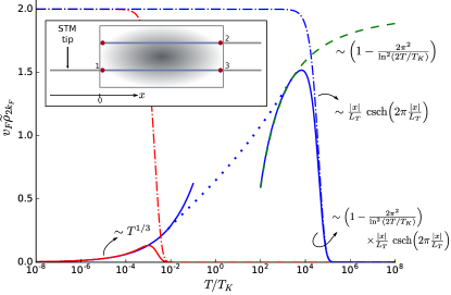
As in any Kondo system, important characteristics of strong correlations are revealed by the conduction electrons’ spatial organization (i.e., the Kondo screening cloudSørensen and Affleck (1996); Barzykin and Affleck (1996); Affleck and Simon (2001); Simon and Affleck (2003); Borda (2007); Affleck et al. (2008); Affleck (2010)) and their scattering properties. Here we focus on a quantity that provides information on both of these: the oscillating (as a function of position) part of the local electron tunneling density of states (tDOS), specifically its thermally smeared form motivated by scanning tunneling microscopy (STM). (For works focusing on the complementary nonoscillating part, see Ref. Eriksson et al., 2014b; Agarwal et al., 2009.) We will see that, unlike for free fermions, the amplitude of the oscillating tDOS component does not increase monotonically as temperature is lowered, but follows a form that depends on the position of the tunneling point relative to the Kondo cloud (see Fig. 1). While the nonmonotonic temperature dependence is already indicative of strongly correlated scattering, strikingly, we also find that at the topological Kondo fixed point, in contrast even to correlated Fermi liquids,Nozieres (1974); Nozieres and Blandin (1980) single-particle scattering becomes completely suppressed, and that this translates into the complete suppression of the oscillating part of the tDOS as the temperature (and bias voltage) tends to zero. Furthermore, for the minimal three-lead setup that we will focus on, the features that we predict can be turned off by decoupling any of the leads other than the one in which the tDOS is measured, which provides a direct signature of the Majorana fermion nonlocality.
II General Considerations
We now turn to formulating the problem for our tDOS calculations. There are three terms that contribute to the Hamiltonian,Béri and Cooper (2012); Galpin et al. (2014)
| (1) |
The first term is due to the noninteracting, effectively spinless, conduction electrons in the three metallic leads (see Fig. 1),
| (2) |
where is the Fermi velocity. (The velocities can be taken to be the same for all leads without loss of generality.de C. Chamon and Fradkin (1997)) We are working at sufficiently low energies, so that we can focus on the vicinity of Fermi wavenumber where the lead electron spectrum can be considered linear. The electron operator in momentum space can be related to that in position space through
| (3) |
where is the spatial coordinate in each lead such that the Majorana-lead junction is located at . The eigenfunction of the -th lead (in the absence of Majorana-lead coupling) takes the form
| (4) |
where and are the right and left movers, respectively, and is the reflection amplitude of electrons at the lead endpoint.
Working at energies much below the induced superconducting gap, the superconducting island is characterized by the charging energy through the term
| (5) |
where is the number operator of the electrons in the island, is the background charge, and is the electron charge.Nazarov and Blanter (2009) The distance between any two Majorana zero modes is assumed to be large enough to ensure that the overlap of their localized wavefunctions can be ignored. In this case, the only tunneling mechanism we consider is when the electron of lead tunnels into the island through the Majorana with amplitude , which is taken to be positive without loss of generality. The Hamiltonian for this is
| (6) |
where is an operator that changes the number of electrons in the island, .Fu (2010); Béri and Cooper (2012)
We will be focusing on energy scales much smaller than , so that the physics is dominated by virtual transitions connecting the lowest energy charge state to the neighboring ones. Focusing on the middle of the Coulomb blockade valley for simplicity (i.e., setting to be an integer multiple of in ), this physics can be described by the effective Hamiltonian , where
| (7) |
with where is the Levi-Civita matrix.Béri and Cooper (2012); Béri (2013); Galpin et al. (2014) This is the Kondo coupling mediating the interaction between the spin- topological qubit described by the operators and the conduction electrons. The three lead species of the latter form an effective spin- density .Béri and Cooper (2012)
As stated in the Introduction, we focus on the thermally smeared local tDOS of lead electrons, proportional to the STM differential conductance,Bruus and Flensberg (2004)
| (8) |
where is the Fermi function, is the applied voltage between the STM tip and the lead, is the temperature, and is the electron spectral function. The latter can be calculated through the relation , where is the retarded Green’s function, obtained from the Matsubara Green’s function,
| (9) |
with (imaginary) time-ordering operator , by performing an analytic continuation from the upper half plane to the real axis, .Bruus and Flensberg (2004) Note that at zero temperature, the tDOS is simply .
It is customary to introduce the so-called Kondo screening cloud, which is defined as the Kondo contribution to tDOS: If denotes the tDOS of lead electrons when uncoupled from the Majoranas (which will be called the free cloud in the rest of the paper), then the Kondo cloud is defined by .
The retarded Green’s function can be written in terms of the -matrix , which is a key object encoding Kondo correlations,Affleck and Ludwig (1993); Affleck (2010)
| (10) | |||
Here is the retarded Green’s function in the absence of interaction between electrons and Majoranas. This free Green’s function is obtained by performing the analytic continuation of Eq. (9), except that the averaging is performed by using the eigenstates of the noninteracting Hamiltonian instead.Affleck and Ludwig (1993) It has the form
| (11) | |||||
| (12) |
where
| (13) |
Due to the relation we have .Affleck and Ludwig (1993)
A convenient parametrization of the -matrix is
| (14) |
where the is present because only the diagonal terms survive the average over the impurity spin inherent in the definition of the Green’s function. The angle (with odd integer) is excluded because in this case the electron operator at the Majorana-lead junction vanishes, and therefore so does the Kondo coupling.
Note that since enters multiplicatively in Eq. (10), the spatial features for are entirely due to and . To look for spatial features providing information on Kondo correlations we will therefore mostly focus on and for simplicity mostly take . In this zero bias regime, the free cloud has a simple expression,
| (15) | |||
where is the thermal length.
As exemplified by and above, all quantities of our interest have two contributions: a nonoscillating and a -oscillating component. For the rest of the paper, we focus only on the latter because this is the piece that involves both ingoing and outgoing waves and thus encodes information about the scattering properties. [In contrast, at least for noninteracting lead electrons, the nonoscillating part is insensitive to the Kondo coupling as seen from Eqs. (10)-(12).] Denoting the oscillating components by the subscript , we have
| (16) |
A key step in calculating the tDOS is thus the calculation of . In the following, we will focus on two complementary regimes: high energies [] and low energies [], where is the Kondo temperature [see Sec. III below], considering mostly the zero bias case. These two regimes correspond to the vicinity of two renormalization group (RG) fixed points around which a perturbation theory can be developed: the free electron fixed point () for high energies and the topological Kondo fixed point for low energies. In the high energy regime, the function will be obtained using perturbation theory in the Kondo couplings , considering terms up to third order. For low energies, we will adapt conformal field theory (CFT) results from Ref. Affleck and Ludwig, 1993 to our model.
III -tDOS at High Energies
After performing perturbation theory up to third order in the Kondo couplings, one finds
| (17) |
with cutoff and dimensionless couplings
| (18) |
For , Eq. (17) can be approximated asCheung and Mattuck (1970)
| (19) |
To gain some insight into the behavior of , one may conveniently recast Eq. (19) using the weak coupling RG flowBéri and Cooper (2012); Altland and Egger (2013); Béri (2013); Galpin et al. (2014) (and its cyclic permutations). Up to , i.e., to the accuracy of our perturbation expansion, one finds
| (20) |
where is as in Eq. (18), but now in terms of the running couplings . The latter satisfy , where is the Kondo temperature, the single, emergent, energy scale characterizing the system and separating high and low energies. To the accuracy of our RG equations, it is given byBéri and Cooper (2012); Altland and Egger (2013); Béri (2013); Galpin et al. (2014) , where is the typical (bare) value of the couplings. (We have in the isotropic case.) As the weak coupling RG equations are the same as those for the conventional Kondo effect, it follows that the high-energy expression Eq. (19), apart from an overall factor, is the same as that for ordinary single-channel Kondo systems,Affleck (2010) which can be represented by the lead-dot model to be discussed later (see Fig. 4a).
Using our results for , we now discuss the high-energy form of the Kondo cloud and the oscillating tDOS. The essential features are already captured by the simplest, isotropic, case which we focus on henceforth. The Kondo cloud at zero bias is given by
| (21) | |||||
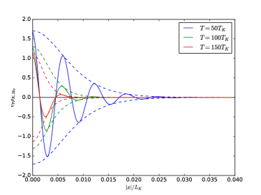
for (see the Appendix for details). This is depicted in Fig. 2 for various temperatures as a function of , where is the Kondo length. Also shown is the amplitude of , denoted as . (The temperatures used in Fig. 2 may strictly be somewhat outside the domain where perturbation theory is accurate,Galpin et al. (2014) but we believe that apart from overestimating the amplitude, the graph captures well the behavior.) The exponential suppression of the function in the limit is manifested in two complementary aspects: for fixed , it shows that decays exponentially with increasing on the scale of , and, for fixed , given that in Eq. (15) contains the same function, one sees that it governs the exponential decay of the high temperature tail of the tDOS amplitude shown in Fig. 1. (The function itself, describing both the envelope of the Kondo cloud apart from the logarithmic factor and the envelope for the free cloud, is shown as a function of in Fig. 3 bottom panel, with dash-dotted.)
The temperature dependence of and is particularly interesting when there is a good scale separation so that . In this case, the high energy regime displays a crossover upon lowering the temperature, from the exponential behavior discussed above for to a regime where is governed by the Kondo logarithm. Extrapolating our results to beyond the perturbative regime we expect this logarithm-like increase of the Kondo cloud to develop into a contribution comparable to the free cloud and thus to govern the behaviour of itself. Conversely, for , the Kondo cloud and remain exponentially suppressed even for , thus the high temperature regime crosses over to the low temperature one without an intermediate logarithmic behavior. The temperature dependence of in these two complementary regimes is shown in Fig. 1. The presence versus the suppression of the logarithmic contribution may be used to estimate , that is, the extent of the Kondo screening cloud.
IV -tDOS at Low Energies
Now we turn to energies much below . In this regime, weak perturbation theory is inapplicable. Instead, we will work in the vicinity of the topological Kondo fixed pointBéri and Cooper (2012) and adapt the CFT results of Ref. Affleck and Ludwig, 1993 to obtain . At the Kondo fixed point, i.e., at zero energy where the RG-irrelevant perturbations near this fixed point completely decayed, we have
| (22) |
where is the single-particle-to-single-particle scattering amplitude at the Fermi energy. It is given by
| (23) |
with , where is the level of the SU current algebra, is the spin of conduction electrons, and is the impurity spin.Affleck and Ludwig (1993) For our model, , , and ,Béri and Cooper (2012); Galpin et al. (2014) and therefore . This remarkable result signifies that, in stark contrast to Fermi liquid behavior, there is no single-particle scattering in topological Kondo systems at the Kondo fixed point. In terms of , which measures the single electron interference of incoming and outgoing waves, the vanishing of at the Kondo fixed point translates into as . The -tDOS thus may be used to directly demonstrate the absence of single-particle scattering in the topological Kondo effect.
At low energies, but away from the Kondo fixed point, RG-irrelevant perturbations have to be taken into account and these lead to corrections to the function . For the neighborhood of an SU non-Fermi liquid Kondo fixed point, considering only the perturbation of the smallest scaling dimension (the leading irrelevant operator), the CFT calculation of Ref. Affleck and Ludwig, 1993 shows that where is an integral expression. (Note that in contrast to the description in the high energy regime, the CFT does not determine , but it rather enters as a microscopic parameter: it is the high energy cutoff of the low energy theory.) For the details of the calculation and the resulting general form of we refer the reader to Ref. Affleck and Ludwig, 1993; here we only use the result specialized for the case of the three-lead topological Kondo effect.Béri and Cooper (2012) We have
| (24) |
Here is proportional to the dimensionless coupling of the leading irrelevant operator and
| (25) | |||||
where is the gamma function and is the hypergeometric function. We emphasize that the power law in Eq. (24) directly informs on the the scaling dimension .
For low energies, it is useful to consider two complementary regimes: when but , and when with . Though as mentioned earlier, the spatial correlations are due to the free Green’s functions, there is useful information to be obtained from and the overall amplitude of . For we find
| (26) |
where and is the sign function. This expression, firstly, may be used to specify : while this is a free parameter for the CFT, the fact that the -matrix is a universal functionGalpin et al. (2014) of implies that also has a universal value. We can approximately obtain this by using Eq. (26) to fit to the numerically exact results of Ref. Galpin et al., 2014; this gives . It also follows that for , is a simple expression set by the second term in Eq. (26):
| (27) | |||
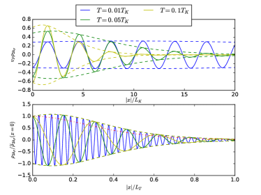
In the , case, we plot the oscillating component of the tDOS of lead electrons for various temperatures (top panel of Fig. 3). As the function of temperature, is gradually suppressed for all as decreases. This is in contrast to the free cloud which gradually saturates upon lowering the temperature [see Eq. (15) and Fig. 1]. Note that at low energies, since became the short distance cutoff (as follows from being the high energy cutoff), the only length scale that can set long distance features is the thermal length . This can be made manifest by noting that the tDOS amplitude , as shown in the Appendix, admits the scaling form with the universal scaling function . The corresponding scaling collapse, illustrated in the bottom panel of Fig. 3, may serve as a useful characteristic of the spatial organization of conduction electrons near the topological Kondo fixed point, and as means to demonstrate the law (and thus the scaling dimension ) governing the suppression of the oscillations as the temperature is lowered (Fig. 1). [Extracting and thus the scaling function from in practice may be facilitated by oscillation extrema much denser than , including . The latter is not inconsistent with being the short distance cutoff of the CFT, since that only limits the spatial resolution for , and not the wavelength of the oscillations.] We note that a similar form, , holds also in the high energy regime. The scaling function in that case, , is however the same as for free fermions and thus unlike for low energies, does not provide information on Kondo features. The two curves are contrasted in the bottom panel of Fig. 3.
V Discussion and Conclusions
A common feature shared by our high- and low-temperature results is the thermal-length-controlled large- decay of the amplitude [see Eqs. (15) and (21) and Fig. 3]. In terms of the temperature dependence of (illustrated in Fig. 1), the role of is thus to control the competition between the thermal and Kondo lengths and by setting the low temperature cutoff above which dominates.
Considering that our high- and low-energy asymptotics are expected to be accurateGalpin et al. (2014) for and , respectively, one needs slightly exaggerated values to achieve good scale separation while staying within the strict domain of validity of our theory. (Fig. 1 uses for and for .) We however believe that the behavior is captured qualitatively correctly also for less conservative values of , as in Figs. 2, 3, which allows for scale separation for more moderate . It would be interesting to compare this expectation to results from numerical renormalization group calculations of the -matrix which are valid also between the asymptotic regimes.Mitchell et al. (2011)
To work in the regime dominated by topological Kondo physics, as we noted in Sec. II, temperature and voltage should be much smaller than the induced superconducting gap and the charging energy . For topological Kondo setups, these are expected to be comparable to those in recent Al-InAs nanowire devicesAlbrecht et al. (2016, 2017); Sestoft et al. (2018) where . These values also provide an estimate for the energy window within which to set the Kondo temperature using suitable tunnel couplings. For clear oscillations, low disorder leads with mean free path satisfying are advantageous, as in recent ballistic InSb nanowireZhang et al. (2017b) and InAs 2DEG basedLee et al. (2017) devices with , considering a typical Fermi wavelengthJespersen et al. (2009) of . In terms of the oscillation amplitude itself, as shown in Fig. 1, these are appreciable: the maximal amplitude (as the function of ), even for , is just an order of magnitude smaller than that of the saturated () free tDOS, and it increases with decreasing . Provided that the free tDOS is accessible in the device components forming the leads, the features we predict should also be visible.
While in Sec. III we found that the high energy behavior of and is similar to that in more conventional Kondo systems, there are important differences in the low energy regime. It is thus useful to contrast our results to such more conventional, single- and multi-channel Kondo systems. The simplest, single-channel Kondo effect arises in the lead-dot model shown Fig. 4a. Here , corresponding to a phase shift in single-particle scattering.Nozieres (1974); Affleck and Ludwig (1993) This system is a local Fermi liquid at low energies. The low temperature thus is similar to the free cloud, increasing upon lowering temperature as the reduction of thermal smearing allows more and more single-particle interference.
Our findings are also in contrast with two-channel Kondo (2CK) systems proposed and later experimentally studied by Oreg and Goldhaber-Gordon.Oreg and Goldhaber-Gordon (2003); Potok et al. (2007) Their system is a two-lead 2CK model where there is a linear combination of modes without single-particle scattering at the Fermi energy [i.e., for this linear combination], but there is another linear combination which still has single-particle scattering, translating into at the 2CK fixed point.Carmi et al. (2012) It is interesting to note, however, that one may modify this model by removing one of the leads while maintaining the coupling symmetry between the remaining lead and the large dot (leading to the setup in Fig. 4b). Now there is only the mode, which leads to at the 2CK fixed point. However, as temperature is lowered, the power-law suppression is different: , as can be shown by adapting our considerations to this case.
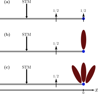
A system for which we do find the same power law (and SU current algebraFabrizio and Gogolin (1994)) as for the topological Kondo effect is the 4CK model, corresponding to the generalized Oreg-Goldhaber-Gordon setup with three large dotsOreg and Goldhaber-Gordon (2003); Florens and Rosch (2004) (Fig. 4c). However, now the conduction electrons have , which results in and thus at the 4CK fixed point.
Generalizing our considerations, it is also interesting to note that one may use at zero temperature and bias to measure in a range of Kondo and other quantum impurity systems, provided there is only one value of to consider (as is the case for single channel leads). To this end, one takes the ratio between and the nonoscillating tDOS component . This is useful since the proportionality factor [originating from Eq. (8)] is the same in both cases and depends only on the density of states and physical characteristics of the STM tip.Bruus and Flensberg (2004); Gottlieb and Wesoloski (2006) Therefore, .
To summarize, we have shown that the oscillating component of the tDOS provides valuable novel insights into the strong correlations in the topological Kondo effect. At zero bias, the difference in the behavior of the amplitude as a function of temperature for different values of provides information on the size of the Kondo length , and hence the extent of the Kondo screening cloud. At low temperatures, admits a universal scaling form characterizing the conduction electrons’ spatial organization near the topological Kondo fixed point. As temperature and bias tend to zero, becomes completely suppressed, revealing that in the topological Kondo effect, single-particle scattering is entirely absent at the Fermi energy.
Acknowledgements
We thank S. Das and V. Dwivedi for input at early stages of the work, and R. Egger and M. Galpin for useful discussions. This research was supported by the Royal Society, the Indonesian Endowment Fund for Education (LPDP) scholarship, the EPSRC grant EP/M02444X/1, and the ERC Starting Grant No. 678795 TopInSy.
Appendix
In this Appendix, we study the temperature dependence of the amplitude of the -tDOS with isotropic couplings at zero bias, both in the high and low energy regimes. If one denotes , in the high energy regime the spectral function contribution relevant for the Kondo cloud amplitude has the form
| (28) | |||
The Kondo cloud then can be obtained from Eq. (8). For , its amplitude can be approximated by the integral
Since for , this shows that the amplitude of the Kondo cloud decays exponentially with on the scale .
In the low energy regime, one has
| (30) | |||
Therefore, the amplitude of the -tDOS is
| (31) |
for some function . To extract the asymptotic power law, we may take , and thus substitute . This gives the decay.
References
- Wilczek (2009) F. Wilczek, Nat. Phys. 5, 614 (2009).
- Alicea (2012) J. Alicea, Rep. Prog. Phys. 75, 076501 (2012).
- Beenakker (2013) C. Beenakker, Ann. Rev. Cond. Mat. Phys. 4, 113 (2013).
- Kitaev (2003) A. Y. Kitaev, Ann. Phys. (Berlin) 303, 2 (2003).
- Nayak et al. (2008) C. Nayak, S. H. Simon, A. Stern, M. Freedman, and S. Das Sarma, Rev. Mod. Phys. 80, 1083 (2008).
- Stern (2010) A. Stern, Nature 464, 187 (2010).
- Alicea (2010) J. Alicea, Phys. Rev. B 81, 125318 (2010).
- Oreg et al. (2010) Y. Oreg, G. Refael, and F. von Oppen, Phys. Rev. Lett. 105, 177002 (2010).
- Kitaev (2001) A. Y. Kitaev, Physics-Uspekhi 44, 131 (2001).
- Lutchyn et al. (2010) R. M. Lutchyn, J. D. Sau, and S. Das Sarma, Phys. Rev. Lett. 105, 077001 (2010).
- Leijnse and Flensberg (2012) M. Leijnse and K. Flensberg, Semicond. Sci. Technol. 27, 124003 (2012).
- Mourik et al. (2012) V. Mourik et al., Science 336, 1003 (2012).
- Albrecht et al. (2016) S. M. Albrecht et al., Nature 531, 206 (2016).
- Zhang et al. (2017a) H. Zhang et al., arXiv:1710.10701 (2017a).
- Nadj-Perge et al. (2013) S. Nadj-Perge, I. K. Drozdov, B. A. Bernevig, and A. Yazdani, Phys. Rev. B 88, 020407 (2013).
- Nadj-Perge et al. (2014) S. Nadj-Perge et al., Science 346, 602 (2014).
- Kjærgaard et al. (2016) M. Kjærgaard et al., Nat. Commun. 7, 12841 (2016).
- Nichele et al. (2017) F. Nichele et al., Phys. Rev. Lett. 119, 136803 (2017).
- Das et al. (2012) A. Das, Y. Ronen, Y. Most, Y. Oreg, M. Heiblum, and H. Shtrikman, Nat. Phys. 8, 887–895 (2012).
- Deng et al. (2012) M. T. Deng et al., Nano Lett. 12, 6414 (2012).
- Finck et al. (2013) A. D. K. Finck, D. J. Van Harlingen, P. K. Mohseni, K. Jung, and X. Li, Phys. Rev. Lett. 110, 126406 (2013).
- Law et al. (2009) K. T. Law, P. A. Lee, and T. K. Ng, Phys. Rev. Lett. 103, 237001 (2009).
- Flensberg (2010) K. Flensberg, Phys. Rev. B 82, 180516 (2010).
- Sau et al. (2010) J. D. Sau, S. Tewari, R. M. Lutchyn, T. D. Stanescu, and S. Das Sarma, Phys. Rev. B 82, 214509 (2010).
- Wimmer et al. (2011) M. Wimmer, A. R. Akhmerov, J. P. Dahlhaus, and C. W. J. Beenakker, New J. Phys. 13, 053016 (2011).
- Zazunov et al. (2016) A. Zazunov, R. Egger, and A. Levy Yeyati, Phys. Rev. B 94, 014502 (2016).
- Bagrets and Altland (2012) D. Bagrets and A. Altland, Phys. Rev. Lett. 109, 227005 (2012).
- Pikulin et al. (2012) D. I. Pikulin, J. P. Dahlhaus, M. Wimmer, H. Schomerus, and C. W. J. Beenakker, New J. Phys. 14, 125011 (2012).
- Liu et al. (2012) J. Liu, A. C. Potter, K. T. Law, and P. A. Lee, Phys. Rev. Lett. 109, 267002 (2012).
- Kells et al. (2012) G. Kells, D. Meidan, and P. W. Brouwer, Phys. Rev. B 86, 100503 (2012).
- Rainis et al. (2013) D. Rainis, L. Trifunovic, J. Klinovaja, and D. Loss, Phys. Rev. B 87, 024515 (2013).
- Hasan and Kane (2010) M. Z. Hasan and C. L. Kane, Rev. Mod. Phys. 82, 3045 (2010).
- Qi and Zhang (2011) X.-L. Qi and S.-C. Zhang, Rev. Mod. Phys. 83, 1057 (2011).
- Fu (2010) L. Fu, Phys. Rev. Lett. 104, 056402 (2010).
- Béri and Cooper (2012) B. Béri and N. R. Cooper, Phys. Rev. Lett. 109, 156803 (2012).
- Altland and Egger (2013) A. Altland and R. Egger, Phys. Rev. Lett. 110, 196401 (2013).
- Béri (2013) B. Béri, Phys. Rev. Lett. 110, 216803 (2013).
- Galpin et al. (2014) M. R. Galpin et al., Phys. Rev. B 89, 045143 (2014).
- Altland et al. (2014a) A. Altland, B. Béri, R. Egger, and A. M. Tsvelik, J. Phys. A: Math. Theor. 47, 265001 (2014a).
- Altland et al. (2014b) A. Altland, B. Béri, R. Egger, and A. M. Tsvelik, Phys. Rev. Lett. 113, 076401 (2014b).
- Zazunov et al. (2014) A. Zazunov, A. Altland, and R. Egger, New J. Phys. 16, 015010 (2014).
- Eriksson et al. (2014a) E. Eriksson, C. Mora, A. Zazunov, and R. Egger, Phys. Rev. Lett. 113, 076404 (2014a).
- Eriksson et al. (2014b) E. Eriksson, A. Nava, C. Mora, and R. Egger, Phys. Rev. B 90, 245417 (2014b).
- Plugge et al. (2016) S. Plugge, A. Zazunov, E. Eriksson, A. M. Tsvelik, and R. Egger, Phys. Rev. B 93, 104524 (2016).
- Herviou et al. (2016) L. Herviou, K. Le Hur, and C. Mora, Phys. Rev. B 94, 235102 (2016).
- Zazunov et al. (2017) A. Zazunov, F. Buccheri, P. Sodano, and R. Egger, Phys. Rev. Lett. 118, 057001 (2017).
- Béri (2017) B. Béri, Phys. Rev. Lett. 119, 027701 (2017).
- Michaeli et al. (2017) K. Michaeli, L. A. Landau, E. Sela, and L. Fu, Phys. Rev. B 96, 205403 (2017).
- Gau et al. (2018) M. Gau, S. Plugge, and R. Egger, Phys. Rev. B 97, 184506 (2018).
- Nozieres and Blandin (1980) P. Nozieres and A. Blandin, J. Phys. 41, 193 (1980).
- Affleck (1990) I. Affleck, Nucl. Phys. B 336, 517 (1990).
- Affleck and Ludwig (1991a) I. Affleck and A. Ludwig, Nucl. Phys. B 352, 849 (1991a).
- Affleck and Ludwig (1991b) I. Affleck and A. Ludwig, Nucl. Phys. B 360, 641 (1991b).
- Affleck et al. (1992) I. Affleck, A. Ludwig, H. Pang, and D. Cox, Phys. Rev. B 45, 7918 (1992).
- Oreg and Goldhaber-Gordon (2003) Y. Oreg and D. Goldhaber-Gordon, Phys. Rev. Lett. 90, 136602 (2003).
- Potok et al. (2007) R. M. Potok, I. G. Rau, H. Shtrikman, Y. Oreg, and D. Goldhaber-Gordon, Nature 446, 167 (2007).
- Iftikhar et al. (2018) Z. Iftikhar et al., Science 360, 1315 (2018).
- Sørensen and Affleck (1996) E. S. Sørensen and I. Affleck, Phys. Rev. B 53, 9153 (1996).
- Barzykin and Affleck (1996) V. Barzykin and I. Affleck, Phys. Rev. Lett. 76, 4959 (1996).
- Affleck and Simon (2001) I. Affleck and P. Simon, Phys. Rev. Lett. 86, 2854 (2001).
- Simon and Affleck (2003) P. Simon and I. Affleck, Phys. Rev. B 68, 115304 (2003).
- Borda (2007) L. Borda, Phys. Rev. B 75, 041307 (2007).
- Affleck et al. (2008) I. Affleck, L. Borda, and H. Saleur, Phys. Rev. B 77, 180404 (2008).
- Affleck (2010) I. Affleck, in Perspectives Of Mesoscopic Physics: Dedicated to Yoseph Imry’s 70th Birthday (World Scientific, 2010) pp. 1–44.
- Agarwal et al. (2009) A. Agarwal, S. Das, S. Rao, and D. Sen, Phys. Rev. Lett. 103, 026401 (2009).
- Nozieres (1974) P. Nozieres, J. Low Temp. Phys. 17, 31 (1974).
- de C. Chamon and Fradkin (1997) C. de C. Chamon and E. Fradkin, Phys. Rev. B 56, 2012 (1997).
- Nazarov and Blanter (2009) Y. V. Nazarov and Y. M. Blanter, Quantum Transport: Introduction to Nanoscience (Cambridge University Press, 2009).
- Bruus and Flensberg (2004) H. Bruus and K. Flensberg, Many–Body Quantum Theory in Condensed Matter Physics (Oxford University Press, 2004).
- Affleck and Ludwig (1993) I. Affleck and A. W. W. Ludwig, Phys. Rev. B 48, 7297 (1993).
- Cheung and Mattuck (1970) C. Y. Cheung and R. D. Mattuck, Phys. Rev. B 2, 2735 (1970).
- Mitchell et al. (2011) A. K. Mitchell, M. Becker, and R. Bulla, Phys. Rev. B 84, 115120 (2011).
- Albrecht et al. (2017) S. M. Albrecht et al., Phys. Rev. Lett. 118, 137701 (2017).
- Sestoft et al. (2018) J. E. Sestoft et al., Phys. Rev. Materials 2, 044202 (2018).
- Zhang et al. (2017b) H. Zhang et al., Nat. Commun. 8, 16025 (2017b).
- Lee et al. (2017) J. S. Lee et al., arXiv:1705.05049 (2017).
- Jespersen et al. (2009) T. S. Jespersen, M. Polianski, C. Sørensen, K. Flensberg, and J. Nygård, New J. Phys. 11, 113025 (2009).
- Carmi et al. (2012) A. Carmi, Y. Oreg, M. Berkooz, and D. Goldhaber-Gordon, Phys. Rev. B 86, 115129 (2012).
- Fabrizio and Gogolin (1994) M. Fabrizio and A. O. Gogolin, Phys. Rev. B 50, 17732 (1994).
- Florens and Rosch (2004) S. Florens and A. Rosch, Phys. Rev. Lett. 92, 216601 (2004).
- Gottlieb and Wesoloski (2006) A. D. Gottlieb and L. Wesoloski, Nanotechnology 17, R57 (2006).