Effect of payload size on mean response time when message segmentations occur using queueing model
Abstract
This paper proposes the queueing model to represent arrivals of segmented packets when message segmentations occur. This queueing model enables us to derive the closed form of mean response time, given payload size, message size distribution and message arrival rate. From a numerical result, we show that the mean response time is more convex in payload sizes if message arrival rate is larger in a scenario where Web objects are delivered over a physical link.
Index Terms:
Message segmentation, payload size, response time, queueing model.I Introduction
The size of packets, i.e., data units transferred over physical links, affects several quality of service (QoS) parameters for users of packet-based transfer networks such as the Internet. For example, the response time between hosts is highly dependent on packet size because it contains link-level transmission time, which is simply given by the packet size divided by capacity of the physical link [1, p. 9]. In addition, the packet-loss rate due to bit errors depends on the packet size because it is approximately proportional to the packet size [2, p. 132].
The packet size is limited for various reasons [3, pp. 406–409]. They include a) the data-link structure (e.g., the width of a transmission slot), b) compliance with standard protocol specifications, and c) satisfaction of the QoS parameters by applications such that the round-trip time of interactive applications is less than the time that a user is willing to wait [4, 5].
Messages, i.e., data units generated by applications, are frequently larger than the maximum permitted packet size. To convey such messages over the network, some communication protocols, such as transmission control protocol (TCP), Internet protocol (IP) for the Internet [6], IEEE 802.11 media access control (MAC) protocol [7] for wireless local-area networks (LANs) and radio link control (RLC) protocol [8] for mobile wide-area networks, specify a message segmentation/reassembly function. The message segmentation function enables a sender to divide a single message larger than the payload size into multiple packets. Furthermore, the sender adds an appropriate header, i.e., overhead, to a packet.
There have been several studies on optimization of packet size (or payload size) to satisfy the user’s QoS such as [9, 10, 11]. However, the purpose of these studies was to solve the tradeoff issue between the desire to reduce the header overhead by making packet large, and the need to reduce packet-loss rate due to bit errors in noisy links by using small packet size.
Another tradeoff exists when message segmentations occur. Consider the message whose variance is large enough in size, such as Web files (objects). While too large payload size is employed, message segmentations hardly occur. In this case, the waiting times of packets for transmission using a physical link is large because the packet size distribution can be identified with the message size distribution. On the other hand, when payload size is small, waiting times of packets may be small due to decreasing the variance of packet sizes because the constant packets in size, which is payload size, are dominant in the all created packets. When payload size is too small, the number of segmented packets per message increases significantly, resulting in very large waiting time due to the burstiness of packet arrivals.
In previous work, this tradeoff issue has not been discussed. The purpose of this paper is to discuss the effect of payload size on mean response time when message segmentations occur using an queueing model [12, Chapter 4], which can capture the behavior of the burstiness of segmented packet arrivals.
The rest of the paper is organized as follows. In the next section, we describe the communication network model underlying our study. Section III analyzes the segmented packet sequence. Section IV derives the closed form of mean response time using an queueing model. Section V investigates the effect of message segmentation on the mean response time for actual message size distributions. Finally, Section VI summarizes this paper and mentions future work.
II Communication network model
In this section, we first explain the two-layered communication network model under consideration. Next, the model of data units introduced in this paper at the respective layer is described. In final, we explain some assumptions for analytical tractability.
II-A Layer model
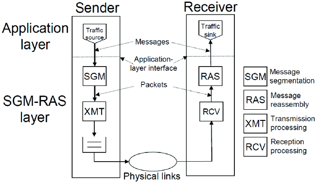
To investigate the effect of message segmentation on performance, we consider a communication network of which conceptual representation is shown in Fig. 1. Each station (a sender and a receiver) has two layers: application and segmentation-reassembly (SGM-RAS).
The application layer contains a traffic source and sink. The traffic source generates the data units, which will be referred to as messages. On the other hand, the traffic sink terminates the corresponding data units.
The SGM-RAS layer implements message SGM-RAS function. In addition, it has a function to transfer data units, which will be referred to as packets, over physical links at a sender.
II-B Data-unit model
We define data units exchanged between peer entities at the respective layer: messages and packets.
-
Message: a data unit generated by a traffic source with a given size distribution,
-
Packet: a data unit created from a message through segmentation function by adding a header and/or trailer, i.e., control information, to the (divided) message. The message segmentation function implemented in the sender’s SGM-RAS layer enables a single message to be divided into several packets if the message size is larger than the payload size . The receiver’s SGM-RAS layer performs a message reassembly function, thus reassembling the segmented generated packets before delivering them to the application layer.
II-C Assumptions
For analytical tractability, we make the following assumptions.
- A1:
-
message sizes are mutually independent and identically distributed according to a common message-size distribution . The distribution has a finite mean value , which is referred to as the mean message size.
- A2:
-
the finite variance of the message-size distribution exists.
III Segmented packet sequence model
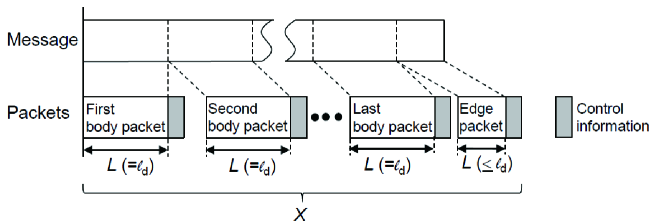
The creation of packets from a message through message segmentation is shown in Fig. 2. If a message is larger than payload size , the message is divided into multiple packets. Two kinds of packets exist:
-
body packet: a segmented packet appearing between the head and the penultimate packets in the original message, whose packet size is always equal to , and
-
edge packet: the final segmented packet if a message is segmented, or the message itself if it is not segmented, whose packet size is variable but does not exceed .
Let a random variable be a packet size excluding control information (header). Letting be the stationary distribution of packet sizes, we have
| (1) |
where is the stationary edge-packet-size distribution and is the edge packet occurrence probability. The form of is given by
| (2) |
The form of can be written as
| (3) |
Here, the term is defined as
| for , | (4) |
with , and we regard that when .
Letting be the mean packet size, from (1) and assumption of A1, the form of is given by
| (5) |
Let be the variance of packet sizes. From (1) and assumption of A2, the variance of packet sizes is given by
| (6) |
where
| for , | (7) |
with .
Let a random variable be the number of packets created from a corresponding message. Note that the random variable is identified with a batch size, which will be introduced in Section IV.
The forms of and are given by
| (8) |
| (9) |
IV Mean response time
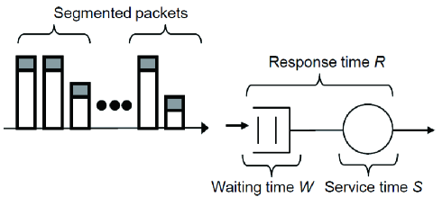
In this paper, we employ the response time as the performance. To derive the form of , we represent a communication network as a queueing system as shown in Fig. 3. The response time is defined as the total time from a packet arrival at the queue until its service completion. In the communication network, a service time in a queueing system where the server is a physical link is equal to transmission time, which is given by where a data unit is in size and is the capacity of the physical link. The response time is interpreted as the waiting time , i.e., time spent in the queue alone, plus the service time .
For analytical tractability, we introduce the following assumptions:
- B1:
-
packets created from a corresponding message, referred to as a batch, arrive at the queueing system simultaneously at a time.
- B2:
-
the batches arrive at the queueing system according to Poisson process with mean arrival rate .
- B3:
-
the maximum number of packets that can be accommodated in the queueing system is infinite.
- B4:
-
packets are served in FIFO scheduling dripline.
- B5:
-
offered load satisfies .
- B6:
-
the size of SGM-RAS-layer’s control information is constant and equal to .
From assumptions of B1 – B4, we can treat the queueing system as an queueing model in the Kendall notation, where is the batch size, which is defined as the number of packets simultaneously arriving at the queueing system.
From assumption of B5, the becomes stable.
By solving the queueing model, we have
| (10) | ||||
| (11) | ||||
| (12) | ||||
| (13) |
V Numerical results and discussions
In this section, we examine the effect of payload size on mean response time by utilizing the results in Section IV. We consider a scenario in which Web objects are transferred over the IEEE 802.11g, i.e., physical link capacity Mbps and control information field size bytes.
The sizes of the Web objects are assumed to follow a lognormal distribution given by
| (14) |
The distribution parameters and are assumed to be and , respectively, on the basis of the measured mean message size bytes and the measured standard deviation bytes [14]. Note that this lognormal distribution can represent a long-tailed property.
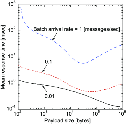
Figure 4 shows mean response time versus payload sizes for different batch arrival rates . This figure demonstrates the mean response time is convex in payload sizes .
The reason for this is as follows.
-
•
When payload size is large enough
From (4), for is approximately zero, resulting in . Hence, message segmentations hardly occur.
In addition, it yields and . Hence, since batch size is approximately one, the queueing system can be approximated as an queueing model
The mean waiting time for the queueing model is given by
(15) From the above equation, we find that mean response time depends on the coefficient of variation of , , that is, . If , equivalently the variance of message sizes in proportional, increases, increases. In this example, the value of is very high because the message size distribution exhibits long-tailed property.
-
•
When payload size is small
When payload size decreases, the number of segmented packets per message increases, resulting in the smaller value of . Hence, the mean response time may be smaller if payload size is smaller even though the mean batch size increases.
-
•
When payload size is small enough
In this case, the segmented packets, of which size is is dominant in all created packets. Therefore, the queueing system can be approximated as an queueing model. Although the value of is almost zero, the mean batch size is too large, resulting in large mean response time.
From Fig. 4, we find that the mean response time is more convex in payload sizes if batch arrival rate is larger.
VI Conclusion
This paper proposed the queueing model to discuss the effect of payload size on mean response time when message segmentations occur. We derived the closed form of mean response time, given payload size, message size distribution and message arrival rate. From a numerical result, we have demonstrated that the mean response time is more convex in payload sizes if message arrival rate is larger. in a scenario where Web objects are delivered over a physical link.
The remaining issues include the clarification of the relationship among several parameters to express the optimized payload size, the extension of our model to noisy links, and development of payload adaptation algorithm to minimize the mean response time.
Acknowledgment
This work was supported by JSPS KAKENHI Grant Number JP15K00139.
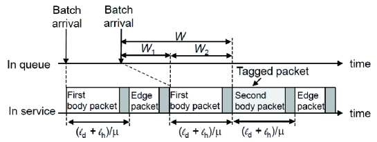
To derive (IV), we observe an arbitrary packet in a batch (i.e., message), referred to as the tagged packet, and divide the waiting time into two parts (see Fig. 5):
-
•
waiting time : the time from when the first packet in a batch have the tagged packet arrives at the queueing system to when it enters service.
-
•
waiting time : the time from when the first packet enters service to when the tagged packet enters service.
From the argument of [12, Chapter 4], the form of is given by
| (16) |
Noting that one message consists of consecutive body packets and an edge packet when it it is divided to packets (see Fig. 2), we have
| (17) |
because of . From (16) and (Acknowledgment), we obtain (IV).
References
- [1] H. Kobayashi and B. Mark, System Modeling and Analysis: Foundations of System Performance Evaluation. Prentice Hall, 2008.
- [2] M. Schwartz, Telecommunication Networks: Protocols, Modeling and Analysis. Addison-Wesley Publishing Company, 1987.
- [3] A. S. Tanenbaum, Computer Networks, 3rd ed. Prentice Hall PTR, 1996.
- [4] G. Montenegro, S. Dawkins, M. Kojo, V. Magret, and N. Vaidya, Long Thin Networks. Network Working Group Request for Comments, Jan. 2000, no. RFC 2757.
- [5] S. Dawkins, G. Montenegro, M. Kojo, and V. Magret, End-to-end Performance Implications of Slow Links. Network Working Group Request for Comments, July 2001, no. RFC 3150.
- [6] W. R. Stevens, TCP/IP Illustrated, Volume 1: The Protocols. Addison-Wesley Publishing Company, 1994.
- [7] B. P. Crow, I. Widjaja, J. G. Kim, and P. T. Sakai, “IEEE 802.11 wireless local area networks,” IEEE Communications Magazine, vol. 35, no. 9, pp. 116–126, Sept. 1997.
- [8] 3rd Generation Partnership Project, “Technical Specification Group Radio Access Network; Radio Link Control (RLC) protocol specification,” [Online]. Available: http://www.3gpp.org/, 2005.
- [9] P. Lettieri and M. Srivastava, “Adaptive frame length control for improving wireless link throughput, range, and energy efficiency,” in Proc. IEEE INFOCOM’98, 1998, pp. 564–571.
- [10] E. Modiano, “An adaptive algorithm for optimizing the packet size used in wireless ARQ protocols,” Journal Wireless Networks, vol. 5, no. 4, pp. 279–286, July 1999.
- [11] P. R. Jelenković and J. Tan, “Dynamic packet fragmentation for wireless channels with failures,” in Proc. ACM MobiHoc’08, 2008, pp. 73–82.
- [12] H. Akimaru and K. Kawashima, Teletraffic: Theory and Applications. Springer-Verlag, 1993.
- [13] T. Ikegawa, Y. Kishi, and Y. Takahashi, “Data-unit-size distribution model when message segmentations occur,” Performance Evaluation, vol. 69, no. 1, pp. 1–16, Jan. 2012.
- [14] M. Molina, P. Castelli, and G. Foddis, “Web traffic modeling exploiting TCP connections’ temporal clustering through HTML-REDUCE,” IEEE Network, vol. 14, no. 3, pp. 46–55, May/June 2000.