Theory and computation of electromagnetic fields and thermomechanical structure interaction for systems undergoing large deformations
The post-print version of the manuscript:
B.E. Abali, A.F. Queiruga, J. Comput. Phys. (2019), pp. 1–32
https://doi.org/10.1016/j.jcp.2019.05.045

Abstract

For an accurate description of electromagneto-thermomechanical systems, electromagnetic fields need to be described in a Eulerian frame, whereby the thermomechanics is solved in a Lagrangean frame. It is possible to map the Eulerian frame to the current placement of the matter and the Lagrangean frame to a reference placement. We present a rigorous and thermodynamically consistent derivation of governing equations for fully coupled electromagneto-thermomechanical systems properly handling finite deformations. A clear separation of the different frames is necessary. There are various attempts to formulate electromagnetism in the Lagrangean frame, or even to compute all fields in the current placement. Both formulations are challenging and heavily discussed in the literature. In this work, we propose another solution scheme that exploits the capabilities of advanced computational tools. Instead of amending the formulation, we can solve thermomechanics in the Lagrangean frame and electromagnetism in the Eulerian frame and manage the interaction between the fields. The approach is similar to its analog in fluid structure interaction, but more challenging because the field equations in electromagnetism must also be solved within the solid body while following their own different set of transformation rules. We additionally present a mesh-morphing algorithm necessary to accommodate finite deformations to solve the electromagnetic fields outside of the material body. We illustrate the use of the new formulation by developing an open-source implementation using the FEniCS package and applying this implementation to several engineering problems in electromagnetic structure interaction undergoing large deformations.

1 Introduction

The theory of electromagnetism started with Maxwell (1892) and is often explained by Maxwell’s equations. The theory has been continuously developed and amended, notably in the 1950s during the so-called renaissance of thermodynamics. The inclusion of mechanics and thermodynamics into the theory of electromagnetism can be modeled by using balance equations; however, there is no consensus about the correct form of the balance equations among the scientific community. The lack of consensus owes to various challenges in the formulation and the lack of experimental verifications for proposed formulations. For example, there are different representations of Maxwell’s equations, cf. Pao and Hutter (1975) and (Chu et al., 1966, Sect. II). Another challenge occurs due to the different invariance properties of balance laws and Maxwell’s equations, raising questions about the proper forms of electromagnetic interaction equations in matter. The readers are directed to (Truesdell and Toupin, 1960, §286) for some of these different formulations.

In addition to agreeing upon the balance equations for electromagneto-thermomechanical fields, we must also define the constitutive responses, i.e., the equations modeling the material behavior. Typically, phenomenological equations are constructed relying on experiments, which limit their applicability to the particular conditions of the measurement conditions. In order to define generic relations, we want to follow a consistent theoretical derivation through thermodynamics. However, there is no consensus for deriving thermodynamically sound constitutive equations for electromagnetically polarizable systems. The challenge again lies in the formulation of balance equations, especially on the balance of energy, which has been discussed by Ericksen (2007) as well as in Steigmann (2009). There exist a few complete theories for polarized deformable media, as those of (de Groot and Mazur, 1984, Chap. XIII), (Müller, 1985, Chap. 9), (Eringen and Maugin, 1990, Chap. 5), (Kovetz, 2000, Chap. 15), Brechet and Ansermet (2014), and (Abali, 2016, Chap. 3). Each of the mentioned formulations is different, and an experimental verification to determine their correctness is still missing.

Computational methods help us to simulate and comprehend realistic applications in two ways. First, we can estimate the response of a system before manufacturing. Secondly, we can design experiments for validating or even discovering an accurate representation of the physical world. Several computational strategies exist for solving coupled equations by means of finite element simulations. For detailed reviews, see Benjeddou (2000), Hachkevych and Terlets’kyi (2004), and Vidal et al. (2011). Different simplifications of the governing equations are employed in order to enable a numerical analysis. Especially solving coupled problems involves numerical challenges and different numerical treatments are proposed for solving coupled problems, see Chung et al. (2014); Jin (2015); Gil and Ortigosa (2016); Dorfmann and Ogden (2017); Assous et al. (2017); Demkowicz (2017); Pierrus (2018). Different length and time scales are incorporated for a possible modeling in Zäh and Miehe (2015); Schroeder et al. (2016); Zhang and Oskay (2017); Keip and Schröder (2018). Combining different numerical techniques also yields feasible methods in computational modeling, see Liu et al. (2016); Liu and Trung (2016); Nedjar (2017); Kraus et al. (2017); Lanteri et al. (2018); Kodjo et al. (2019). General formulations for thin structures are studied in Klinkel et al. (2013); Staudigl et al. (2018); Chróścielewski et al. (2018). For example, restriction to the quasi-static case by neglecting inertial terms can be seen in Yi et al. (1999), Ahmad et al. (2006) and Queiruga and Zohdi (2016b). A case without free charges was presented by Svendsen and Chanda (2005). A magneto-elasto-static case has been suggested in Spieler et al. (2014), Glane et al. (2017). In Mehnert et al. (2017) the temperature distribution is also computed by neglecting inertial terms. A complete dynamical description and transient computation of electromagneto-thermomechanical has been proposed in Queiruga and Zohdi (2016a) and Abali and Reich (2017). In most of these works, the formulations are established on the same configuration. If the electromagnetic fields interact with solid bodies, a Lagrangean frame is chosen, where each coordinate maps to a material particle. In the case of fluids, a Eulerian frame is chosen, wherein each coordinate indicates a fixed position in ordinary (physical) space. Solving electromagnetic fields in a Eulerian frame and thermomechanical fields in a Lagrangean frame is not a new idea. Among others, Kankanala and Triantafyllidis (2004); Rieben et al. (2007); Stiemer et al. (2009); Barham et al. (2010); Steinmann (2011); Skatulla et al. (2012); Vogel et al. (2013); Ethiraj and Miehe (2016); Pelteret et al. (2016) have developed computational strategies to overcome different problems. In all aforementioned works, governing equations differ due to the different simplifications and assumptions used. Instead of a comparison of different works, we start from the beginning with a new derivation of the equations based on continuum mechanics such that any assumptions and weaknesses in the methodology can be precisely identified and addressed.

We begin by outlining the theory in Section 2, following (Abali, 2016, Chap. 3) most closely. The main objective is to compute the primitive variables for solids under finite deformation, namely the temperature $T$ and displacement $\bm{u}$, and to compute for the entirety of space encompassed by the computational domain the so-called electromagnetic potentials $\phi$, $\bm{A}$. In the formulation we will use different frames, where $\bm{X}$ denotes the reference position of a massive particle, and $\bm{x}$ indicates a position in the ordinary space. The formulation referring to the placement of particles in $\bm{X}$ is called the Lagrangean frame (placement, configuration). Thermomechanical fields belong to massive particles such that they are computed in the Lagrangean frame, which allows to incorporate large deformations for a material system. Electomagnetic fields propagate in $\bm{x}$ with or without interacting with material such that their formulation is developed in the Eulerian frame (configuration), which is tantamount to the control volume for an open system. In order to close the formulation, we develop thermodynamically consistent constitutive equations for solids in Section 3. The theory is limited to elastic materials; plasticity is not treated. The constitutive equations are developed for polarized materials such that all coupling effects, including piezo-and pyroelectric and thermal expansion, are captured precisely. Therefore, the formulation gives rise to coupled and nonlinear field equations to be solved. We discuss the issues that arise when solving these equations using the finite element method in Section 4. In order to address the large deformations of the mesh of the solid body embedded in the mesh of the electromagnetic computational domain, we present a mesh morphing algorithm that enables the calculations by keeping a valid mesh in the space surrounding the body. The variational forms and new algorithms are implemented with the aid of the novel collection of open-source packages provided by the FEniCS project (Hoffman et al., 2005; Logg et al., 2011). The library containing the presented mesh morphing algorithm and other helper routines is released at https://github.com/afqueiruga/afqsfenicsutil under the GNU Lesser General Public License (GNU Public, 2007). In Section 5, we present three simulations of example applications to electromagnetic devices. The simulation setups and FEM implementations of the variational forms are published at https://github.com/afqueiruga/EMSI-2018 under the GNU General Public License. We conclude the discussion in Section 6.

2 Governing equations

Consider a solid body $\mathscr{b}$ immersed in air. We will solve electromagnetic fields in the whole domain $\Omega$ including a body $\mathscr{b}$ and air, $\Omega_{\textrm{air}}=\Omega\backslash\mathscr{b}$. The solid body undergoes a deformation. The mechanical fields will be computed within the body $\mathscr{b}$. Although the surrounding air might be set in motion due to the deformation of the solid body and its own electromagnetic interactions, we will ignore the fluid motion. For certain applications, we might want to determine the temperature distribution within the air as well, but it is not of interest for now. We choose to compute the temperature distribution only within the solid body to save computational time. Therefore, we aim at determining governing equations for electromagnetic fields within $\Omega$ and for thermomechanical fields within $\mathscr{b}$. At the interface $I=\Omega\cap\partial\mathscr{b}$, we need to discuss the interaction and model by satisfying an additional set of equations derived in a rational approach. We motivate the theory in three subsections:

• specifying the partial differential equations modeling electromagnetic fields in the whole domain;

• specifying the partial differential equations describing thermomechanical fields in the solid body; and

• specifying the jump conditions on the interface between the solid body and its surroundings.

We will use Cartesian coordinates and the usual tensor index notation with the Einstein summation convention over repeated indices. Note that different typefaces will be used to denote the electromagnetic fields measured in different frames.

2.1 Electromagnetic fields

The main objective in electromagnetism is to obtain the electric field, $\bm{E}$, and the magnetic flux density, $\bm{B}$ (an area density). SI units are the most appropriate choice for thermomechanical couplings, where the electric field is measured in V(olt)/m(eter) and the magnetic flux density is measured in T(esla). We start off with Faraday’s law:

$$\begin{gathered}\bigg{(}\int_{S}\mathscr{B}_{i}\,\mathrm{d}a_{i}\bigg{)}^{\scalebox{0.4}{\textbullet}}=-\int_{\partial\mathcal{S}}\mathscr{E}_{i}\,\mathrm{d}\ell_{i}\ ,\end{gathered}$$ (1)

defined on an arbitrarily moving surface $S$ with the electric field measured on the co-moving frame, $\boldsymbol{\mathscr{E}}$, as well as the magnetic flux on the co-moving frame, $\boldsymbol{\mathscr{B}}$. In other words, the measurement device is installed on $S$ and moves with it. The notation $\left(\right)^{\scalebox{0.4}{\textbullet}}$ denotes rate regarding the motion of the surface $S$. Assume that the domain $S$ defined in $\bm{x}$ moves with the velocity $\bm{x}^{\scalebox{0.4}{\textbullet}}=\bm{w}$ measured with respect to the laboratory frame that is set to be fixed (not moving). In order to define a velocity as a measurable quantity, we have to declare one frame without possessing a velocity. Of course, a laboratory frame on Earth moves with respect to other planets and stars; however, we declare and maintain the laboratory frame as being fixed such that every motion detected in that frame acquires a well-defined velocity. Since $\boldsymbol{\mathscr{B}}$ and $\boldsymbol{\mathscr{E}}$ are detected on a moving frame, we need their transformations to the laboratory frame,

$$\begin{gathered}\mathscr{E}_{i}=E_{i}+(\bm{w}\times\bm{B})_{i}\ ,\quad\mathscr{B}_{i}=B_{i}\ ,\end{gathered}$$ (2)

for the non-relativistic case, where the magnitude of the domain velocity is small with respect to the speed of light in vacuum, $|\bm{w}|\ll c$. By using Stokes’s theorem as well as the identity for the derivative of a differential area

$$\begin{gathered}(\,\mathrm{d}a_{i})^{\scalebox{0.4}{\textbullet}}=\Big{(}\frac{\partial w_{k}}{\partial x_{k}}\delta_{ji}-\frac{\partial w_{j}}{\partial x_{i}}\Big{)}\,\mathrm{d}a_{j}\ ,\end{gathered}$$ (3)

we acquire the local form of Faraday’s law:

$$\begin{gathered}B^{\scalebox{0.4}{\textbullet}}_{j}+B_{i}\Big{(}\frac{\partial w_{k}}{\partial x_{k}}\delta_{ji}-\frac{\partial w_{j}}{\partial x_{i}}\Big{)}=-\operatorname{curl}(\bm{E}+\bm{w}\times\bm{B})_{j}\ ,\\ \frac{\partial B_{j}}{\partial t}+\frac{\partial B_{j}}{\partial x_{k}}w_{k}+B_{j}\frac{\partial w_{k}}{\partial x_{k}}-B_{i}\frac{\partial w_{j}}{\partial x_{i}}+\epsilon_{jkl}\frac{\partial E_{l}}{\partial x_{k}}+\epsilon_{jkl}\epsilon_{lmn}\frac{\partial w_{m}B_{n}}{\partial x_{k}}=0\ ,\\ \frac{\partial B_{j}}{\partial t}+\frac{\partial B_{j}w_{k}}{\partial x_{k}}-B_{i}\frac{\partial w_{j}}{\partial x_{i}}+\epsilon_{jkl}\frac{\partial E_{l}}{\partial x_{k}}+\frac{\partial w_{j}B_{k}}{\partial x_{k}}-\frac{\partial w_{k}B_{j}}{\partial x_{k}}=0\ ,\\ \frac{\partial B_{j}}{\partial t}+\epsilon_{jkl}\frac{\partial E_{l}}{\partial x_{k}}+w_{j}\frac{\partial B_{k}}{\partial x_{k}}=0\ ,\end{gathered}$$ (4)

using the identity $\epsilon_{jkl}\epsilon_{lmn}=\delta_{jm}\delta_{kn}-\delta_{jn}\delta_{km}$ with the Kronecker delta, $\delta_{ij}$, and the Levi-Civita symbol, $\epsilon_{ijk}$. Moreover, we can consider the special case where the surface $S$ is a closed hull, for example the boundary of a continuum body, $\partial\mathscr{b}$, without a line boundary such that the right-hand side in Eq. (1) vanishes and we obtain after an integration in time

$$\begin{gathered}\int_{\partial\mathscr{b}}B_{i}\,\mathrm{d}a_{i}=\text{const.}|_{t}\ .\end{gathered}$$ (5)

If we select the initial magnetic flux as zero, the integration constant drops. Since the selected boundary is a closed hull, we can apply Gauss’s law and acquire

$$\begin{gathered}\frac{\partial B_{i}}{\partial x_{i}}=0\ .\end{gathered}$$ (6)

We have obtained the so-called first set of Maxwell’s equations:

$$\begin{gathered}\frac{\partial B_{i}}{\partial x_{i}}=0\ ,\quad\frac{\partial B_{i}}{\partial t}+\epsilon_{ijk}\frac{\partial E_{k}}{\partial x_{j}}=0\ .\end{gathered}$$ (7)

These equations are universal; i.e., they hold for any material and even in the case of no massive particles (vacuum). Hence, the coordinate $\bm{x}$ denotes a location or point in the (ordinary) space. We call it a spatial frame since the coordinates indicate a position in space. There might be a massive particle occupying the location $\bm{x}$, but the coordinate still indicates a location in space without any relation to that particle or its motion. The sought-after electromagnetic fields, $\bm{E}$ and $\bm{B}$, have to satisfy the latter equations. Their solution is obtained by using the following ansatz functions:

$$\begin{gathered}E_{i}=-\frac{\partial\phi}{\partial x_{i}}-\frac{\partial A_{i}}{\partial t}\ ,\quad B_{i}=\epsilon_{ijk}\frac{\partial A_{k}}{\partial x_{j}}\ ,\end{gathered}$$ (8)

such that now we search for the electric potential $\phi$ in V and magnetic potential $\bm{A}$ in T m for $\forall\bm{x}\in\Omega$. If we can compute the electromagnetic potentials, we readily obtain the electromagnetic fields from the latter equations. Since we aim to describe the system using only four components $\{\phi,A_{1},A_{2},A_{3}\}$ instead of six components $\{E_{1},E_{2},E_{3},B_{1},B_{2},B_{3}\}$, there are two scalar degrees of freedom that are not uniquely determined; namely $\partial\phi/\partial t$ and $\partial A_{i}/\partial x_{i}$ can be chosen freely. This so-called gauge freedom can be used to eliminate many numerical problems (Baumanns et al., 2013). We will use Lorenz’s gauge:

$$\begin{gathered}\frac{\partial\phi}{\partial t}=-c^{2}\frac{\partial A_{i}}{\partial x_{i}}\ ,\quad c^{2}=\frac{1}{\mu_{0}\varepsilon_{0}}\ ,\end{gathered}$$ (9)

with the speed of light in vacuum, $c$, defined by the precisely known universal constants:

$$\begin{gathered}\varepsilon_{0}=8.85\cdot 10^{-12}\,\text{A\,s/(V\,m)}\ ,\quad\mu_{0}=12.6\cdot 10^{-7}\,\text{V\,s/(A\,m)}\ .\end{gathered}$$ (10)

In order to motivate the second set of Maxwell’s equations, we use the balance of electric charge in an open system with the control volume or domain $\Omega$ where the domain moves with velocity $\bm{w}$

$$\begin{gathered}\bigg{(}\int_{\Omega}q\,\mathrm{d}v\bigg{)}^{\scalebox{0.4}{\textbullet}}=\int_{\partial\Omega}\Big{(}q(w_{i}-v_{i})-\mathscr{J}_{i}\Big{)}\,\mathrm{d}a_{i}\ .\end{gathered}$$ (11)

The electric charge density, $q$ in C(oulomb)/m³, can be determined if we have a constitutive equation for the electric current (area density), $\boldsymbol{\mathscr{J}}$ in A(mpere)/m². If a massive particle conveying an electric charge of $q$ enters the domain, the amount of charge within the domain increases. The particle moves with $\bm{v}$ and can enter the domain only across its boundary $\partial\Omega$. The particle is entering if the relative velocity $\bm{w}-\bm{v}$ is positive along the surface direction, $\,\mathrm{d}a_{i}=n_{i}\,\mathrm{d}a$ and exiting if it is in the other direction. We refer to Müller and Muschik (1983), Muschik and Müller (1983) for a discussion of balance equations in an open system with a moving domain. The surface direction $\bm{n}$ points outward from the domain. We can again get the local form after using the rate of the volume element in the spatial frame moving with $\bm{w}$,

$$\begin{gathered}\,\mathrm{d}v^{\scalebox{0.4}{\textbullet}}=\frac{\partial w_{i}}{\partial x_{i}}\,\mathrm{d}v\ ,\end{gathered}$$ (12)

and apply Gauss’s law,

$$\begin{gathered}q^{\scalebox{0.4}{\textbullet}}+q\frac{\partial w_{i}}{\partial x_{i}}=\frac{\partial}{\partial x_{i}}\Big{(}q(w_{i}-v_{i})-\mathscr{J}_{i}\Big{)}\ ,\\ \frac{\partial q}{\partial t}+\frac{\partial qw_{i}}{\partial x_{i}}=\frac{\partial}{\partial x_{i}}\Big{(}q(w_{i}-v_{i})-\mathscr{J}_{i}\Big{)}\ ,\\ \frac{\partial q}{\partial t}+\frac{\partial J_{i}}{\partial x_{i}}=0\ ,\end{gathered}$$ (13)

where $J_{i}=\mathscr{J}_{i}+qv_{i}$ represents the electric current measured in the laboratory frame. Since the domain $\Omega$ has a well-defined boundary, $\partial\Omega$, we can introduce a charge potential $\boldsymbol{\mathscr{D}}$ measured on the moving domain as follows

$$\begin{gathered}\int_{\Omega}q\,\mathrm{d}v=\int_{\partial\Omega}\mathscr{D}_{i}\,\mathrm{d}a_{i}\ ,\end{gathered}$$ (14)

leading to the following Maxwell equation after applying Gauss’s law

$$\begin{gathered}q=\frac{\partial\mathscr{D}_{i}}{\partial x_{i}}\ .\end{gathered}$$ (15)

(Note the typeface on the quantity $\mathscr{D}$.) The charge potential $\boldsymbol{\mathscr{D}}$ in C/m² is quite general and stemming from the total charge $q$ in space. The charge potential is also called dielectric displacement or electrical flux density in the literature. We emphasize that $\boldsymbol{\mathscr{D}}$ is the total charge potential incorporating bound and free charges. Now by using the charge potential, we rewrite the balance of charge in an open domain with a closed boundary, $\partial\partial\Omega=\{\}$,

$$\begin{gathered}\bigg{(}\int_{\partial\Omega}\mathscr{D}_{i}\,\mathrm{d}a_{i}\bigg{)}^{\scalebox{0.4}{\textbullet}}=\int_{\partial\Omega}\Big{(}q(w_{i}-v_{i})-\mathscr{J}_{i}\Big{)}\,\mathrm{d}a_{i}\ ,\end{gathered}$$ (16)

as a balance equation on a surface with its boundary $\partial S$

$$\begin{gathered}\bigg{(}\int_{S}\mathscr{D}_{i}\,\mathrm{d}a_{i}\bigg{)}^{\scalebox{0.4}{\textbullet}}=\int_{\partial S}\mathscr{H}_{i}\,\mathrm{d}\ell_{i}+\int_{S}\Big{(}q(w_{i}-v_{i})-\mathscr{J}_{i}\Big{)}\,\mathrm{d}a_{i}\ ,\end{gathered}$$ (17)

where the flux on the surface boundary $\boldsymbol{\mathscr{H}}$ is called the current potential (or also magnetic field strength). It is measured on the moving surface. Transformations of the charge and current potentials from the moving frame to the laboratory (fixed) frame read

$$\begin{gathered}\mathscr{D}_{i}=D_{i}\ ,\quad\mathscr{H}_{i}=H_{i}+(\bm{D}\times\bm{w})_{i}\ ,\end{gathered}$$ (18)

for the non-relativistic case. Now we can insert the rate of the area element, apply Stokes’s theorem, and obtain the local form

$$\begin{gathered}D^{\scalebox{0.4}{\textbullet}}_{j}+D_{i}\Big{(}\frac{\partial w_{k}}{\partial x_{k}}\delta_{ji}-\frac{\partial w_{j}}{\partial x_{i}}\Big{)}=\operatorname{curl}(\bm{H}+\bm{D}\times\bm{w})_{j}+qw_{j}-J_{j}\ ,\\ \frac{\partial D_{j}}{\partial t}+\frac{\partial D_{j}}{\partial x_{i}}w_{i}+D_{j}\frac{\partial w_{k}}{\partial x_{k}}-D_{i}\frac{\partial w_{j}}{\partial x_{i}}=\epsilon_{jkl}\frac{\partial H_{l}}{\partial x_{k}}+\epsilon_{jkl}\epsilon_{lmn}\frac{\partial D_{m}w_{n}}{\partial x_{k}}+qw_{j}-J_{j}\ ,\\ \frac{\partial D_{j}}{\partial t}+\frac{\partial D_{j}w_{i}}{\partial x_{i}}-D_{i}\frac{\partial w_{j}}{\partial x_{i}}=\epsilon_{jkl}\frac{\partial H_{l}}{\partial x_{k}}+\frac{\partial D_{j}w_{k}}{\partial x_{k}}-\frac{\partial D_{k}w_{j}}{\partial x_{k}}+\frac{\partial D_{i}}{\partial x_{i}}w_{j}-J_{j}\ ,\\ \frac{\partial D_{j}}{\partial t}=\epsilon_{jkl}\frac{\partial H_{l}}{\partial x_{k}}-J_{j}\ .\end{gathered}$$ (19)

We have obtained the second set of Maxwell’s equations:

$$\begin{gathered}q=\frac{\partial D_{i}}{\partial x_{i}}\ ,\quad\frac{\partial D_{j}}{\partial t}=\epsilon_{jkl}\frac{\partial H_{l}}{\partial x_{k}}-J_{j}\ ,\end{gathered}$$ (20)

which are universal and hold in the whole domain. The measured charge and current potentials on the laboratory frame—$\bm{D}$ and $\bm{H}$ respectively—do not change with respect to a domain velocity $\bm{w}$. Therefore, the domain velocity is arbitrary giving us a freedom to choose the domain velocity to our advantage. Later in the text, we will discuss a method to generate the domain velocity in such a way that the mesh quality remains optimal.

We have reached the following governing equations for the total electric charge, current, and their potentials:

$$\begin{gathered}\frac{\partial q}{\partial t}+\frac{\partial J_{i}}{\partial x_{i}}=0\ ,\quad J_{i}=\mathscr{J}_{i}+qv_{i}\ ,\quad q=\frac{\partial D_{i}}{\partial x_{i}}\ ,\\ \frac{\partial D_{j}}{\partial t}-\epsilon_{jki}\frac{\partial H_{i}}{\partial x_{k}}+J_{j}=0\ .\end{gathered}$$ (21)

The equations need to be used to compute the electromagnetic potentials, $\phi$ and $\bm{A}$. In order to close the equations, the total charge potential and the total current potential need to be expressed in terms of the electromagnetic potentials. The Maxwell–Lorentz aether relations

$$\begin{gathered}D_{i}=\varepsilon_{0}E_{i}\ ,\quad H_{i}=\frac{1}{\mu_{0}}B_{i}\ ,\end{gathered}$$ (22)

augmented by Eq. (8) presents the relation closing the coupled governing equations. These equations will be solved in the whole domain, $\Omega$.

2.2 Thermomechanical fields

Consider a continuum body, $\mathscr{b}$, within the domain $\Omega$. This body consists of massive particles with electric charge. Mass (volume) density $\rho$ and specific charge (per mass) $z$ are material dependent variables. Their initial values are known. The total specific charge $z$ in a material is decomposed as free charge $z^{\text{fr.}}$ and bound charges $z^{\text{bo.}}$ as follows

$$\begin{gathered}z=z^{\text{fr.}}+z^{\text{bo.}}\ .\end{gathered}$$ (23)

Free charges are the valence electrons carrying the electric current effectively in a conductor, they can move large distances. Bound charges are held by the intra-molecular forces and they only move less than the molecular length. Their motions give rise to a decomposition of the charge and current potentials,

$$\begin{gathered}D_{i}=\mathfrak{D}_{i}-P_{i}\ ,\quad H_{i}=\mathfrak{H}_{i}+\mathscr{M}_{i}\ ,\end{gathered}$$ (24)

where the bound charge potential $P_{i}$ is called an electric polarization and the bound current potential $\mathscr{M}_{i}$ is called a magnetic polarization. The minus sign is a convention of the declaration of electric polarization in the atomistic scale. Since we already have introduced the Maxwell–Lorentz aether relation, we need constitutive equations either for $\mathfrak{D}_{i}$ and $\mathfrak{H}_{i}$ or for $P_{i}$ and $\mathscr{M}_{i}$. By using the above definitions we achieve the analogous decomposition for the electric current:

$$\begin{gathered}J_{i}=J_{i}^{\text{fr.}}+J_{i}^{\text{bo.}}\ ,\quad J_{i}^{\text{bo.}}=\frac{\partial P_{i}}{\partial t}+\epsilon_{ijk}\frac{\partial\mathscr{M}_{k}}{\partial x_{j}}\ .\end{gathered}$$ (25)

See A for its well-known derivation.

The massive particles’ initial positions are known and denoted by $\bm{X}$. Effected by mechanical, thermal, and electromagnetic forces, particles at $\bm{X}$ displace as much as $\bm{u}$ and move to $\bm{x}$ such that $\bm{u}=\bm{x}-\bm{X}$ in m. Moreover, it is necessary to compute the temperature $T$ in K(elvin) and electromagnetic potentials of particles. Since we know the initial positions of the (non-congruent) particles, we can use $\bm{X}$ in order to identify the material particles. This configuration uses coordinates indicating material particles’ positions at the reference placement. The reference placement is defined by the vanishing energy, which will be investigated in the next section using thermodynamics. Initially, we start from the reference placement and the amount of particles remains the same. This configuration is called a material system expressed in the Lagrangean frame with $\bm{X}$ denoting the initial placement of particles. In the Lagrangean frame, we search for $\bm{u}$, $T$, as functions in space $\bm{X}$ and time $t$. Their field equations are given by the balance equations at the current placement. As the space, $\bm{X}$, indicates the same particle throughout the simulation, we can introduce the balance equations at the current placement and a transformation between current and initial placement. Therefore, in a material system, we start with balance equations for mass, linear momentum, and energy at the current placement and then determine the field equations in the Lagrangean frame by transformation into the current placement. The equations are finally closed by the constitutive equations. We start off with the general balance equation in a volume

$$\begin{gathered}\bigg{(}\int_{\mathscr{b}}\psi\,\mathrm{d}v\bigg{)}^{\scalebox{0.4}{\textbullet}}=\int_{\partial\mathscr{b}}\Phi_{j}\,\mathrm{d}a_{j}+\int_{\mathscr{b}}k\,\mathrm{d}v+\int_{\mathscr{b}}p\,\mathrm{d}v\ ,\quad\end{gathered}$$ (26)

where rate of the volume density $\psi$ is balanced by the fluxes across the boundary $\Phi_{j}$, volumetric supply terms $k$, and production terms $p$. Mathematically, supply and production terms are identical; however, we handle them separately as we can control supply terms but fail to steer production terms. The general balance equation in Eq. (26) is defined at the current placement, where $\bm{x}$ denotes the current positions of material particles conforming a material system. In other words, the integral measure moves with material particles such that the integration domain is the current placement of the continuum body. We start a simulation with known initial conditions, particles at $\bm{X}$, and compute their motion to $\bm{x}$. The current positions of particles change in time such that $x^{\scalebox{0.4}{\textbullet}}_{i}=v_{i}$. The rate is defined with respect to the material particle. Now, the rate of the infinitesimal volume element (an integral measure) reads

$$\begin{gathered}\,\mathrm{d}v^{\scalebox{0.4}{\textbullet}}=\frac{\partial v_{i}}{\partial x_{i}}\,\mathrm{d}v\ ,\end{gathered}$$ (27)

leading to the following local form after applying Gauss’s law:

$$\begin{gathered}\frac{\partial\psi}{\partial t}+\frac{\partial}{\partial x_{j}}(v_{j}\psi-\Phi_{j})-k=p\ .\end{gathered}$$ (28)

In the local form we write the production term on the right-hand side for a clear separation of conserved quantities. If the production term vanishes, the variable in the balance equation is a conserved quantity. We axiomatically start with the balance equations for the mass, total momentum, and total energy as given in Table 1.

Table 1: Matter and (electromagnetic) field related volume densities in the balance equations and their supply terms, flux terms, and production terms.

$\psi$	$\Phi_{j}$	$k$	$p$
$\rho$	$0$	$0$	$0$
$\rho v_{i}+\mathscr{G}_{i}$	$v_{j}\mathscr{G}_{i}+\sigma_{ji}+m_{ji}$	$\rho f_{i}$	$0$
$\rho e^{\text{\tiny m.}}+e^{\text{\tiny f.}}$	$v_{j}e^{\text{\tiny f.}}+\zeta_{j}+\mathscr{P}_{j}$	$\rho s$	$0$

It is important to emphasize that we assume that mass, total momentum, and total energy are all conserved quantities. We skip a long discussion about the angular momentum and simply assume that the material is non-polar, leading to a vanishing spin density such that the angular momentum reduces to the moment of momentum. In this case, the balance of angular momentum is fulfilled by having a symmetric non-convective flux of linear momentum, $\bm{\sigma}+\bm{m}$. After using Table 1, the balance equations read

$$\begin{gathered}\frac{\partial\rho}{\partial t}+\frac{\partial v_{j}\rho}{\partial x_{j}}=0\ ,\\ \frac{\partial}{\partial t}(\rho v_{i}+\mathscr{G}_{i})+\frac{\partial}{\partial x_{j}}\big{(}v_{j}\rho v_{i}-\sigma_{ji}-m_{ji}\big{)}-\rho f_{i}=0\ ,\\ \frac{\partial}{\partial t}(\rho e^{\text{\tiny m.}}+e^{\text{\tiny f.}})+\frac{\partial}{\partial x_{j}}\big{(}v_{j}\rho e^{\text{\tiny m.}}-\zeta_{j}-\mathscr{P}_{j}\big{)}-\rho s=0\ \end{gathered}$$ (29)

Mass density, $\rho$, has a convective flux, $\bm{v}\rho$, because mass is conveyed by the moving material particles. Total momentum density, $\rho\bm{v}+\boldsymbol{\mathscr{G}}$, consists of a part due to matter, $\rho\bm{v}$, and another part due to the electromagnetic field, $\boldsymbol{\mathscr{G}}$. Matter and the electromagnetic field are coupled; however, we will be decomposing terms by splitting the fields along their interaction. Consider a massive object moving in an electromagnetic field in a way that the electromagnetic field does not alter, i.e., matter and field are independent. Of course, as given in the balance of momentum, the existing field’s rate applies forces on the moving charges and a massive object has usually (bound) electric charges such that its acceleration leads to a change in the velocity, in other words, matter and field are coupled but they are independent. As they are independent, we treat the electromagnetic field and matter separately (independently) in a coupled manner. We can always fix matter and vary the field, and vice versa.

In the balance of momentum, convective flux affects terms related to matter but not field. Non-convective flux of momentum, $\bm{\sigma}+\bm{m}$, is also decomposed into Cauchy’s stress, $\bm{\sigma}$, and an electromagnetic stress, $\bm{m}$. The specific supply term, $\bm{f}$, is the (known) body force because of gravity. Total energy density, $\rho e^{\text{\tiny m.}}+e^{\text{\tiny f.}}$, is decomposed into matter and field energies, as well as non-convective fluxes, $\boldsymbol{\zeta}$ and $\boldsymbol{\mathscr{P}}$, respectively. Again, only the energy due to matter is conveyed by moving massive particles, $\bm{v}\rho e^{\text{\tiny m.}}$, as a convective flux. The specific supply term, $s$, is considered as given. All the other terms will be defined in the following discussion.

In the above formulation, the electromagnetic momentum, stress, energy, and flux are the key terms for the correct interaction. Hence it is customary to introduce the following relations:

$$\begin{gathered}\frac{\partial\mathscr{G}_{i}}{\partial t}=\frac{\partial m_{ji}}{\partial x_{j}}-\mathscr{F}_{i}\ ,\\ \frac{\partial e^{\text{\tiny f.}}}{\partial t}=\frac{\partial\mathscr{P}_{j}}{\partial x_{j}}-\pi\ ,\end{gathered}$$ (30)

where the electromagnetic momentum $\boldsymbol{\mathscr{G}}$ and electromagnetic stress $\bm{m}$ are related to the electromagnetic force (density), $\boldsymbol{\mathscr{F}}$; analogously, electromagnetic energy (density) $e^{\text{\tiny f.}}$ and electromagnetic flux $\boldsymbol{\mathscr{P}}$ are related to an electromagnetic power (density), $\pi$. These mathematical identities might be called balance equations; however, we refrain ourselves from using this terminology, since there is an ongoing discussion in the literature about the correctness of this terminology. It is obvious that we can insert the latter identities and renew the table as in Table 2.

Table 2: Matter related volume densities in the balance equations and their supply terms, flux terms, and production terms.

$\psi$	$\Phi_{j}$	$k$	$p$
$\rho$	$0$	$0$	$0$
$\rho v_{i}$	$\sigma_{ji}$	$\rho f_{i}$	$\mathscr{F}_{i}$
$\rho e^{\text{\tiny m.}}$	$\zeta_{j}$	$\rho s$	$\pi$

We stress these balance equations belong to the quantities related to matter; for the momentum (of matter) and energy (of matter), they read

$$\begin{gathered}\frac{\partial\rho v_{i}}{\partial t}+\frac{\partial}{\partial x_{j}}\big{(}v_{j}\rho v_{i}-\sigma_{ji}\big{)}-\rho f_{i}=\mathscr{F}_{i}\ ,\\ \frac{\partial\rho e^{\text{\tiny m.}}}{\partial t}+\frac{\partial}{\partial x_{j}}\big{(}v_{j}\rho e^{\text{\tiny m.}}-\zeta_{j}\big{)}-\rho s=\pi\ .\end{gathered}$$ (31)

After using the balance of mass and the material derivative

$$\begin{gathered}\frac{\,\mathrm{d}}{\,\mathrm{d}t}=\frac{\partial}{\partial t}+v_{i}\frac{\partial}{\partial x_{i}}\ ,\end{gathered}$$ (32)

they are

$$\begin{gathered}\rho\frac{\,\mathrm{d}v_{i}}{\,\mathrm{d}t}-\frac{\partial\sigma_{ji}}{\partial x_{j}}-\rho f_{i}=\mathscr{F}_{i}\ ,\\ \rho\frac{\,\mathrm{d}e^{\text{\tiny m.}}}{\,\mathrm{d}t}-\frac{\partial\zeta_{i}}{\partial x_{i}}-\rho s=\pi\ ,\end{gathered}$$ (33)

furnishing the consequence that momentum and energy of matter are not conserved quantities in the case of electromagnetism.

The production terms $\boldsymbol{\mathscr{F}}$ and $\pi$ need to be defined in such a way that they vanish if electromagnetic fields are zero. Unfortunately, their definitions are challenging and there exists no consensus in the scientific community; see for example Obukhov (2008); Mansuripur (2010); Griffiths (2012); Bethune-Waddell and Chau (2015). We will propose terms in accordance with Eq. (30), which is the method of derivation used in (Lorentz, 1904, Eq. (15)), (Jones, 1964, Chap. 1), (de Groot and Mazur, 1984, Chap. XIV), (Griffiths, 1999, Chap. 8), (Low, 2004, Sect. 3.3). If the electromagnetic momentum, $\mathscr{G}_{i}$, is defined, then, as a consequence of Eq. (30)₁, we can deduce the electromagnetic stress, $m_{ji}$, and the electromagnetic force density, $\mathscr{F}_{i}$. By following Barnett (2010) we emphasize that different choices are perfectly appropriate. The reasoning can be explained as followed: the manifestation of a force as a contact force leads a term into the electromagnetic stress, whereas as a body force leads to a term causing a momentum rate. In the atomistic scale we know that all electromagnetic forces are contact forces. However, in the macroscopic scale we can observe a momentum change due to the electromagnetic fields such that declaring a body force is also suitable. Any choice of $\boldsymbol{\mathscr{G}}$, $\bm{m}$, and $\boldsymbol{\mathscr{F}}$ is possible as long as the relations in Eq. (30) are fulfilled. Analogously, we can choose an electromagnetic flux, $\boldsymbol{\mathscr{P}}$, leading to the field energy and power. The choices cannot be justified or falsified by experiments, since we cannot detect contact forces and motion independently. Every sensor—used for detecting contact forces—depends on material properties coupling motion with electromagnetism.

Now we introduce a specific (per mass) internal energy, $u$, by decomposing the energy of matter in kinetic and internal energy

$$\begin{gathered}e^{\text{\tiny m.}}=\frac{1}{2}v_{i}v_{i}+u\ .\end{gathered}$$ (34)

By inserting the latter into the balance of energy and using the balance of momentum,

$$\begin{gathered}\rho\frac{\,\mathrm{d}v_{i}}{\,\mathrm{d}t}v_{i}+\rho\frac{\,\mathrm{d}u}{\,\mathrm{d}t}-\frac{\partial\zeta_{j}}{\partial x_{j}}-\rho s=\pi\ ,\\ \Big{(}\frac{\partial\sigma_{ji}}{\partial x_{j}}+\rho f_{i}+\mathscr{F}_{i}\Big{)}v_{i}+\rho\frac{\,\mathrm{d}u}{\,\mathrm{d}t}-\frac{\partial\zeta_{j}}{\partial x_{j}}-\rho s=\pi\ ,\\ \rho\frac{\,\mathrm{d}u}{\,\mathrm{d}t}-\frac{\partial}{\partial x_{j}}\big{(}\zeta_{j}-\sigma_{ji}v_{i}\big{)}-\rho(s-f_{i}v_{i})=\sigma_{ji}\frac{\partial v_{i}}{\partial x_{j}}+\pi-\mathscr{F}_{i}v_{i}\ ,\\ \end{gathered}$$ (35)

we have obtained the balance of internal energy. Obviously, we need to define $\pi$ and $\mathscr{F}_{i}$ before we proceed. Among many different possibilities, the following choice leads to a thermodynamically consistent formulation. Suppose that we simply choose the electromagnetic momentum as follows

$$\begin{gathered}\mathscr{G}_{i}=(\bm{\mathfrak{D}}\times\bm{B})_{i}\ ,\end{gathered}$$ (36)

which is called Minkowski’s momentum. It leads to the following electromagnetic stress and force

$$\begin{gathered}m_{ji}=-\frac{1}{2}\delta_{ji}(H_{k}B_{k}+D_{k}E_{k})+H_{i}B_{j}+D_{j}E_{i}\ ,\\ \mathscr{F}_{i}=\rho zE_{i}+\epsilon_{ijk}J_{j}B_{k}-\epsilon_{ijk}\frac{\partial P_{j}}{\partial t}B_{k}-\epsilon_{ijk}P_{j}\frac{\partial B_{k}}{\partial t}\ ,\end{gathered}$$ (37)

after using Maxwell’s equations, see B for its derivation. Suppose now that we choose the electromagnetic flux as Poynting’s vector

$$\begin{gathered}\mathscr{P}_{i}=\epsilon_{ijk}\mathfrak{H}_{j}E_{k}=\big{(}\bm{\mathfrak{H}}\times\bm{E}\big{)}_{i}\ ,\end{gathered}$$ (38)

in this case, as shown in C, we obtain

$$\begin{gathered}e^{\text{\tiny f.}}=P_{i}E_{i}-B_{i}\mathscr{M}_{i}+\frac{1}{2}\big{(}D_{i}E_{i}+H_{i}B_{i})\ ,\quad\pi=J_{i}^{\text{fr.}}E_{i}-P_{i}\frac{\partial E_{i}}{\partial t}+B_{i}\frac{\partial\mathscr{M}_{i}}{\partial t}\ ,\end{gathered}$$ (39)

The production term due to the field can be rewritten by using the above definition of the electromagnetic force

$$\begin{gathered}\mathscr{F}_{i}v_{i}=\frac{\partial}{\partial x_{j}}\Big{(}(-P_{j}E_{i}+\mathscr{M}_{i}B_{j})v_{i}+\big{(}\bm{\mathfrak{H}}\times\bm{E}\big{)}_{j}\Big{)}+\frac{\partial}{\partial t}\bigg{(}B_{i}\mathscr{M}_{i}-P_{j}E_{j}-\frac{1}{2}D_{j}E_{j}-\frac{1}{2}B_{i}H_{i}\bigg{)}-\\ -(-P_{j}E_{i}+\mathscr{M}_{i}B_{j})\frac{\partial v_{i}}{\partial x_{j}}-\mathscr{E}_{i}\mathscr{J}_{i}^{\text{fr.}}+P_{i}\frac{\,\mathrm{d}E_{i}}{\,\mathrm{d}t}-B_{i}\frac{\,\mathrm{d}\mathscr{M}_{i}}{\,\mathrm{d}t}=\frac{\partial}{\partial x_{j}}\Big{(}(-P_{j}E_{i}+\mathscr{M}_{i}B_{j})v_{i}\Big{)}+\\ \underbrace{+\frac{\partial\mathscr{P}_{j}}{\partial x_{j}}-\frac{\partial e^{\text{\tiny f.}}}{\partial t}}_{\displaystyle\pi}-(-P_{j}E_{i}+\mathscr{M}_{i}B_{j})\frac{\partial v_{i}}{\partial x_{j}}-\mathscr{E}_{i}\mathscr{J}_{i}^{\text{fr.}}+P_{i}\frac{\,\mathrm{d}E_{i}}{\,\mathrm{d}t}-B_{i}\frac{\,\mathrm{d}\mathscr{M}_{i}}{\,\mathrm{d}t}.\end{gathered}$$ (40)

We refer to (Abali, 2016, Sect. 3.5) for its derivation based only on subsequent use of Maxwell’s equations and Maxwell–Lorentz aether relations. Now the balance of internal energy reads

$$\begin{gathered}\rho\frac{\,\mathrm{d}u}{\,\mathrm{d}t}-\frac{\partial}{\partial x_{j}}\Big{(}\zeta_{j}-(\sigma_{ji}-P_{j}E_{i}+\mathscr{M}_{i}B_{j})v_{i}\Big{)}-\rho(s-f_{i}v_{i})=\\ =\big{(}\sigma_{ji}-P_{j}E_{i}+\mathscr{M}_{i}B_{j}\big{)}\frac{\partial v_{i}}{\partial x_{j}}+\mathscr{E}_{i}\mathscr{J}_{i}^{\text{fr.}}-P_{i}\frac{\,\mathrm{d}E_{i}}{\,\mathrm{d}t}+B_{i}\frac{\,\mathrm{d}\mathscr{M}_{i}}{\,\mathrm{d}t}\ .\end{gathered}$$ (41)

We emphasize that this derivation holds for every material; we have only used one assumption and supposed that Minkowski’s choice in Eq. (36) is the correct modeling for the electromagnetic momentum. Other than this assumption, the formulation is quite general such that the balance of internal energy in Eq. (41) holds for every system. Conventionally, the non-convective flux term of the internal energy is called the heat flux:

$$\begin{gathered}-q_{j}=\zeta_{j}-(\sigma_{ji}-P_{j}E_{i}+\mathscr{M}_{i}B_{j})v_{i}\ ,\end{gathered}$$ (42)

with the minus sign appearing because heat pumped into the system (against the surface normal) is declared as a positive work. The supply of the internal energy is a given term and is called the radiant heat:

$$\begin{gathered}r=s-f_{i}v_{i}\ .\end{gathered}$$ (43)

The production term

$$\begin{gathered}\Gamma=(\sigma_{ji}-P_{j}E_{i}+\mathscr{M}_{i}B_{j})\frac{\partial v_{i}}{\partial x_{j}}+\mathscr{E}_{i}\mathscr{J}_{i}^{\text{fr.}}-P_{i}\frac{\,\mathrm{d}E_{i}}{\,\mathrm{d}t}+B_{i}\frac{\,\mathrm{d}\mathscr{M}_{i}}{\,\mathrm{d}t}\ ,\end{gathered}$$ (44)

will be especially useful in the following section for deriving the constitutive equations.

Now by using mass balance and Gauss’s law, we can obtain the global forms of mass, total momentum, and internal energy balance equations in the current placement:

$$\begin{gathered}\bigg{(}\int_{\mathscr{b}}\rho\,\mathrm{d}v\bigg{)}^{\scalebox{0.4}{\textbullet}}=0\ ,\quad\bigg{(}\int_{\mathscr{b}}\rho v_{i}\,\mathrm{d}v\bigg{)}^{\scalebox{0.4}{\textbullet}}=\int_{\partial\mathscr{b}}\sigma_{ji}\,\mathrm{d}a_{j}+\int_{\mathscr{b}}\rho f_{i}\,\mathrm{d}v+\int_{\mathscr{b}}\mathscr{F}_{i}\,\mathrm{d}v\ ,\\ \bigg{(}\int_{\mathscr{b}}\rho u\,\mathrm{d}v\bigg{)}^{\scalebox{0.4}{\textbullet}}=-\int_{\partial\mathscr{b}}q_{i}\,\mathrm{d}a_{i}+\int_{\mathscr{b}}\rho r\,\mathrm{d}v+\int_{\mathscr{b}}\Gamma\,\mathrm{d}v\ \end{gathered}$$ (45)

These balance equations are in the current placement given in $\bm{x}$, but we search for thermomechanical fields as functions in space $\bm{X}$ with the reference placement, in which the mass density, displacement, and temperature are known. As the initial conditions are known, for reference placement we choose the initial placement. The volume and area elements are transformed to the initial placement by

$$\begin{gathered}\,\mathrm{d}v=J\,\mathrm{d}V\ ,\quad\,\mathrm{d}a_{j}=\,\mathrm{d}A_{k}J(\bm{F}^{-1})_{kj}\ ,\end{gathered}$$ (46)

with the deformation gradient and its determinant defined by

$$\begin{gathered}F_{ij}=\frac{\partial x_{i}}{\partial X_{j}}=\frac{\partial u_{i}}{\partial X_{j}}+\delta_{ij}\ ,\quad J=\det(\bm{F})\ .\end{gathered}$$ (47)

Since the volume element in the initial placement is constant in time, after inserting the transformation and using Gauss’s law, we obtain the balance equations in a Lagrangean frame

$$\begin{gathered}\rho J=\text{const.}\big{|}_{t}=\rho_{0}\ ,\\ \rho_{0}\frac{\partial v_{i}}{\partial t}=\frac{\partial}{\partial X_{k}}\Big{(}J(\bm{F}^{-1})_{kj}\sigma_{ji}\Big{)}+\rho_{0}f_{i}+J\mathscr{F}_{i}\ ,\\ \rho_{0}\frac{\partial u}{\partial t}=-\frac{\partial}{\partial X_{k}}\Big{(}J(\bm{F}^{-1})_{kj}q_{j}\Big{)}+\rho_{0}r+J\,\Gamma\ ,\end{gathered}$$ (48)

where each coordinate in space $\bm{X}$ denotes a material particle and $\rho_{0}$ indicates the mass density of particles in the reference placement. We need constitutive equations in order to close these equations such that we can solve for the displacement and temperature.

2.3 On the interface

The formulation of partial differential equations generally makes the implicit assumption that all fields must be described as continuous in space and all conserved quantities are volume densities. However, this restriction is artificial, as it is perfectly valid to discuss an infinitely thin membrane with mass area density and velocity defined upon it, for example. Electromagnetism in particular has situations where this applies. Surface charges and currents are prevalent due to material discontinuities, requiring us to develop descriptions for interfaces in addition to the partial differential equations that can only be applied to “smooth” space. Especially between different materials, we obtain “jump” conditions to be satisfied in order to obtain the correct solution.

We name the boundary of the solid body as the interface in order to avoid a confusion to the domain boundary. The interface evolves due to the deformation. Thermomechanical fields are assumed to be computed such that the current placement of the interface is known. We will develop the equations for a generic singular surface and then restrict to the case that the singular surface is the interface. Regions are 3D objects and surfaces are 2D objects embedded in 3D space.

Consider a surface $S$ and its closure $\bar{S}=S\cup\partial S$ between two different regions $\Omega^{+}$ and $\Omega^{-}$ and their closures $\bar{\Omega}^{+}=\Omega^{+}\cup\partial\Omega^{+}$ and $\bar{\Omega}^{-}=\Omega^{-}\cup\partial\Omega^{-}$ that $\bar{S}=\bar{\Omega}^{+}\cap\bar{\Omega}^{-}$. On the plus side of the surface—toward which the normal $\bm{n}$ points—is the region $\Omega^{+}$ and on the minus side lies $\Omega^{-}$. We use $\Omega^{\pm}=\Omega^{+}\cup\Omega^{-}$ and denote the whole domain $\Omega=\Omega^{\pm}\cup S$ as the surface is within the domain. Its boundary is on the domain’s boundary $\partial S=\partial\Omega\cap\bar{S}$ such that the whole boundary reads $\partial\Omega=\partial\Omega^{\pm}\setminus S$. Note that the boundary of the surface, $\partial S$, is a 1D loop embedded in 3D space. The surface and domain may be moving with a velocity $\bm{w}$ and we search for a balance equation in this open system, i.e., we use a Eulerian frame. Now the general balance equation reads

$$\begin{gathered}\bigg{(}\int_{\Omega^{\pm}}\psi^{V}\,\mathrm{d}v+\int_{S}\psi^{S}\,\mathrm{d}a\bigg{)}^{\scalebox{0.4}{\textbullet}}=\int_{\partial\Omega^{\pm}}\Big{(}(w_{j}-v_{j})\psi^{V}+\Phi^{V}_{j}\Big{)}\,\mathrm{d}a_{j}+\int_{\partial S}\Big{(}\psi^{S}(w_{j}-v_{j})+\Phi^{S}_{j}\Big{)}\,\mathrm{d}\ell_{j}+\\ +\int_{\Omega^{\pm}}\big{(}\rho^{V}k^{V}+p^{V}\big{)}\,\mathrm{d}v+\int_{S}\big{(}\rho^{S}k^{S}+p^{S}\big{)}\,\mathrm{d}a\ ,\end{gathered}$$ (49)

where all volume-related quantities are denoted with a superscript $V$ and surface-related quantities with a superscript $S$. We are only interested in a special case where the surface is an interface. In other words, the surface itself is a fictitious separation without any mass area-density, $\rho^{S}=0$. This restriction allows the following simplification after using the geometric transformations

$$\begin{gathered}\,\mathrm{d}v=J\,\mathrm{d}V\ ,\quad\,\mathrm{d}a_{j}=\,\mathrm{d}A_{k}J(\bm{F}^{-1})_{kj}\ ,\quad\,\mathrm{d}\ell_{j}=F_{jk}\,\mathrm{d}L_{k}\ ,\quad\,\mathrm{d}a=\sqrt{\frac{g}{G}}\,\mathrm{d}A\ ,\end{gathered}$$ (50)

where $g$ and $G$ are the determinant of the surface metric tensor in the current and initial placements, respectively. After transforming to the initial placement, we obtain

$$\begin{gathered}\int_{\Omega^{\pm}}(\psi^{V}J)^{\scalebox{0.4}{\textbullet}}\,\mathrm{d}V=\int_{\partial\Omega^{\pm}}\Big{(}(w_{j}-v_{j})\psi^{V}+\Phi^{V}_{j}\Big{)}J(\bm{F}^{-1})_{kj}\,\mathrm{d}A_{k}+\int_{\partial S}\Phi^{S}_{j}F_{jk}\,\mathrm{d}L_{k}+\\ +\int_{\Omega^{\pm}}\big{(}\rho^{V}k^{V}+p^{V}\big{)}J\,\mathrm{d}V+\int_{S}p^{S}\sqrt{\frac{g}{G}}\,\mathrm{d}A\ .\end{gathered}$$ (51)

For an arbitrary field $f$, Gauss’s law in the initial placement reads

$$\begin{gathered}\int_{\Omega^{\pm}}\frac{\partial f}{\partial X_{k}}\,\mathrm{d}V=\int_{\Omega^{+}}\frac{\partial f}{\partial X_{k}}\,\mathrm{d}V+\int_{\Omega^{-}}\frac{\partial f}{\partial X_{k}}\,\mathrm{d}V=\int_{\partial\Omega^{+}}f\,\mathrm{d}A_{k}+\int_{\partial\Omega^{-}}f\,\mathrm{d}A_{k}=\\ =\int_{\partial\Omega^{+}\setminus S}fN_{k}\,\mathrm{d}A+\int_{S}f^{+}N_{k}^{+}\,\mathrm{d}A+\int_{\partial\Omega^{-}\setminus S}fN_{k}\,\mathrm{d}A+\int_{S}f^{-}N_{k}^{-}\,\mathrm{d}A=\int_{\partial\Omega^{\pm}}fN_{k}\,\mathrm{d}A+\int_{S}\llbracket fN_{k}\rrbracket\,\mathrm{d}A\ ,\end{gathered}$$ (52)

with $f^{+}$ or $f^{-}$ as the limit value from the region $\Omega^{+}$ or $\Omega^{-}$ on the interface and $\bm{N}^{+}$ or $\bm{N}^{-}$ showing outward the region $\Omega^{+}$ or $\Omega^{-}$, respectively. The plane normal $\bm{N}$ is of unit length. We introduce a jump bracket notation, $\llbracket fN_{k}\rrbracket=f^{+}N_{k}^{+}+f^{-}N_{k}^{-}$, by making use of the fact that a unit normal appears on both sides of the surface, $N_{k}=N_{k}^{+}=-N_{k}^{-}$, thus, it is possible to rewrite, $\llbracket fN_{k}\rrbracket=(f^{+}-f^{-})N_{k}^{+}$. The difference between values, $f^{+}-f^{-}$, justifies the name of “jump” brackets. We assume that $\partial S$ is closed (no singularities) such that we can use Stokes’s law with an arbitrary term $f_{k}$ as follows

$$\begin{gathered}\int_{\partial S}f_{k}\,\mathrm{d}L_{k}=\int_{S}\operatorname{curl}(\bm{f})_{k}\,\mathrm{d}A_{k}=\int_{S}\epsilon_{kji}\frac{\partial f_{i}}{\partial X_{j}}\,\mathrm{d}A_{k}\ .\end{gathered}$$ (53)

The general balance equation now reads

$$\begin{gathered}\int_{\Omega^{\pm}}\bigg{(}(\psi^{V}J)^{\scalebox{0.4}{\textbullet}}-\frac{\partial}{\partial X_{k}}\Big{(}\big{(}(w_{j}-v_{j})\psi^{V}+\Phi^{V}_{j}\big{)}J(\bm{F}^{-1})_{kj}\Big{)}-\big{(}\rho^{V}k^{V}+p^{V}\big{)}J\bigg{)}\,\mathrm{d}V=\\ =\int_{S}\bigg{(}-\Big{\llbracket}\Big{(}(w_{j}-v_{j})\psi^{V}+\Phi^{V}_{j}\Big{)}J(\bm{F}^{-1})_{kj}N_{k}\Big{\rrbracket}+\epsilon_{kli}\frac{\partial\Phi^{S}_{j}F_{ji}}{\partial X_{l}}N_{k}+p^{S}\sqrt{\frac{g}{G}}\bigg{)}\,\mathrm{d}A\ .\end{gathered}$$ (54)

The left-hand side of the latter is fulfilled within the continuum body; we need to assure that the right-hand side on the interface is satisfied as well. This restriction leads to the additional equation on the interface

$$\begin{gathered}\Big{\llbracket}\Big{(}(w_{j}-v_{j})\psi^{V}+\Phi^{V}_{j}\Big{)}J(\bm{F}^{-1})_{kj}N_{k}\Big{\rrbracket}=\epsilon_{kli}\frac{\partial\Phi^{S}_{j}F_{ji}}{\partial X_{l}}N_{k}+p^{S}\sqrt{\frac{g}{G}}\ .\end{gathered}$$ (55)

The volume density $\psi^{V}$ is a quantity per volume and its corresponding flux $\Phi^{V}_{j}$ is an area density meaning a quantity per area. Concretely, the volume density is compiled in Table 2: mass density, momentum density, and internal energy density. Analogously, the flux term $\Phi^{S}_{j}$ is a line density and $p^{S}$ is a production term; both of them exist only on the interface. For the mass, we know that neither flux nor production terms exist. Therefore, we assume that interface flux and production vanish such as

$$\begin{gathered}\Big{\llbracket}(w_{j}-v_{j})\rho J(\bm{F}^{-1})_{kj}N_{k}\Big{\rrbracket}=0\ ,\end{gathered}$$ (56)

has to be fulfilled. By setting $w_{i}=v_{i}$ on the interface, we will satisfy the latter condition—in the implementation, this condition corresponds to forcing the computational mesh to follow the interface. There is, however, a flux term for the momentum. In mechanics the surface tension is the stress on the interface, see Cammarata (1994), Vermaak et al. (1968), Mays et al. (1968), Shuttleworth (1950). In the case of electromagnetism, the production term on the interface needs to be calculated. As the volumetric production term is given in Eq. (37)₂, the area production term is due to the surface charges and currents. Surface charges and currents become important in mixtures with adhesion between particles. For a solid body, we simply neglect these effects and obtain the balance of momentum,

$$\begin{gathered}\Big{\llbracket}\Big{(}(w_{j}-v_{j})\rho v_{i}+\sigma_{ji}\Big{)}J(\bm{F}^{-1})_{kj}N_{k}\Big{\rrbracket}=0\ .\end{gathered}$$ (57)

Since $\bm{w}=\bm{v}$ on the interface, the first term drops out leaving

$$\begin{gathered}\Big{\llbracket}\sigma_{ji}J(\bm{F}^{-1})_{kj}N_{k}\Big{\rrbracket}=0\ .\end{gathered}$$ (58)

Analogously, for the balance of internal energy on the interface, we use $\bm{v}=\bm{w}$ and neglect the production as well as the line density flux term (surface heat) such that we obtain

$$\begin{gathered}\big{\llbracket}q_{j}N_{k}J(\bm{F}^{-1})_{kj}\big{\rrbracket}=0\ .\end{gathered}$$ (59)

We may discuss the displacement field as a continuous variable, meaning that the continuum body has no cracks. An analogous argument yields that all primitive variables are continuous and will thus be modeled as such. Moreover, the singular surface is an interface in which the surface normal in the current placement has to be continuous. These assertions of continuity yield the following conditions:

$$\begin{gathered}A_{i}^{+}=A_{i}^{-}\ ,\quad\phi^{+}=\phi^{-}\ ,\quad u_{i}^{+}=u_{i}^{-}\ ,\quad T^{+}=T^{-}\ ,\quad\llbracket n_{j}\rrbracket=\llbracket N_{k}J(\bm{F}^{-1})_{kj}\rrbracket=0\ .\end{gathered}$$ (60)

In the numerical implementation we need to guarantee that the latter equations apply on the interface. This condition is equivalent imposing that all primitive variables—$\bm{A}$, $\phi$, $\bm{u}$, and $T$—are (piecewise) continuous within the whole computational domain. Moreover, by deriving Maxwell’s equations from the balance equations, the following equations are obtained

$$\begin{gathered}\llbracket n_{i}\mathfrak{D}_{i}\rrbracket=0\ ,\quad\llbracket\epsilon_{ijk}n_{j}\mathfrak{H}_{k}\rrbracket=0\ ,\end{gathered}$$ (61)

under the assumption that no surface charges and currents exist. The jump terms emerge due to the difference of material parameters between the adjacent materials. As we use continuous $\bm{A}$, $\phi$ in combination with Eqs. (24), (22), we can also deduce

$$\begin{gathered}\llbracket n_{i}P_{i}\rrbracket=0\ ,\quad\llbracket\epsilon_{ijk}n_{j}\mathscr{M}_{k}\rrbracket=0\ .\end{gathered}$$ (62)

3 Constitutive equations

Various thermodynamical procedures exist in the literature. They all aim at deriving the constitutive equations for $\boldsymbol{\mathscr{J}}^{\text{fr.}}$, $\bm{\sigma}$, $\bm{q}$, $\bm{P}$, and $\boldsymbol{\mathscr{M}}$. We use a similar strategy as in de Groot and Mazur (1984) in which the main assumption is that the internal energy is recoverable, leading to an entropy with primary variables but not fluxes. This assumption is a limitation in the theory; for extension see Jou et al. (1999), Müller and Ruggeri (2013). Moreover, we neglect irreversible effects in polarization such as hysteresis. The presented theory incorporates only elastic materials; in other words, we neglect irreversible deformation called plasticity. Only first gradient of the primitive variables are considered; for higher gradient theories, we refer to Altenbach et al. (2013), Abali et al. (2017).

We will compute the primitive variables in the whole domain: the temperature $T$, displacement $\bm{u}$, electric potential $\phi$, and magnetic potential $\bm{A}$. In the end, every proposed constitutive equation has to depend only on the primitive variables, including their space and time derivatives. Since we have general relations in Eq. (8) between electromagnetic fields, $\bm{E}$, $\bm{B}$, and electromagnetic potentials, $\phi$, $\bm{A}$, we can also define dependencies with respect to $\bm{E}$ and $\bm{B}$. The constitutive equations are necessary where a material occupies a region, they are also called material equations and are defined in the reference (herein initial) placement. We start with Eq. (48)₃, i.e., the balance of internal energy

$$\begin{gathered}\rho_{0}\frac{\partial u}{\partial t}=-\frac{\partial Q_{i}}{\partial X_{i}}+\rho_{0}r+J\Gamma\ ,\quad Q_{i}=J(\bm{F}^{-1})_{ij}q_{j}\ ,\\ \Gamma=\Xi_{ji}\frac{\partial v_{i}}{\partial x_{j}}+\mathscr{E}_{i}\mathscr{J}_{i}^{\text{fr.}}-P_{i}\frac{\,\mathrm{d}E_{i}}{\,\mathrm{d}t}+B_{i}\frac{\,\mathrm{d}\mathscr{M}_{i}}{\,\mathrm{d}t}\ ,\quad\Xi_{ji}=\sigma_{ji}-P_{j}E_{i}+\mathscr{M}_{i}B_{j}\ .\end{gathered}$$ (63)

In the following we will define constitutive equations for $u$, $\bm{Q}$, $\bm{\sigma}$, $\boldsymbol{\mathscr{J}}^{\text{fr.}}$, $\bm{P}$, $\boldsymbol{\mathscr{M}}$. The supply term, $r$, is a given function in space and time. Production of internal energy, $\Gamma$, consists of four terms. The third and fourth terms are crucial for deriving the constitutive equations for $\bm{P}$ and $\boldsymbol{\mathscr{M}}$. The second term in the production of internal energy is called Joule’s heat. We will see this term as a purely dissipative phenomenon. The first term can be rewritten

$$\begin{gathered}J\Xi_{ji}\frac{\partial v_{i}}{\partial x_{j}}=J\Xi_{ji}\frac{\partial v_{i}}{\partial X_{k}}(\bm{F}^{-1})_{kj}=N_{ki}\frac{\partial v_{i}}{\partial X_{k}}\ ,\end{gathered}$$ (64)

with the nominal stress $N_{ji}=J(\bm{F}^{-1})_{jk}\Xi_{ki}$ defined in the initial placement. Moreover, we observe

$$\begin{gathered}\frac{\,\mathrm{d}F_{ij}}{\,\mathrm{d}t}=\frac{\,\mathrm{d}}{\,\mathrm{d}t}\frac{\partial x_{i}}{\partial X_{j}}=\frac{\partial^{2}x_{i}}{\partial t\partial X_{j}}=\frac{\partial^{2}x_{i}}{\partial X_{j}\partial t}=\frac{\partial v_{i}}{\partial X_{j}}\ ,\end{gathered}$$ (65)

such that the balance of internal energy becomes

$$\begin{gathered}\rho_{0}\frac{\partial u}{\partial t}=-\frac{\partial Q_{i}}{\partial X_{i}}+\rho_{0}r+N_{ji}\frac{\,\mathrm{d}F_{ij}}{\,\mathrm{d}t}+J\mathscr{E}_{i}\mathscr{J}_{i}^{\text{fr.}}-JP_{i}\frac{\,\mathrm{d}E_{i}}{\,\mathrm{d}t}+JB_{i}\frac{\,\mathrm{d}\mathscr{M}_{i}}{\,\mathrm{d}t}\ .\end{gathered}$$ (66)

Now we make several assumptions in order to deduce an equation for equilibrium. Since fields do not change in equilibrium, any external supply such as $r$ or production such as Joule’s heat vanishes in equilibrium. In the most general case, we have to assume that the internal energy, heat flux, and electromagnetic polarization have reversible and irreversible parts. First, we assume that the internal energy is fully recoverable, neglecting the irreversible part of the internal energy. This is a conventional method that is appropriate for many engineering systems. We ignore effects of flux rates (the stress rate and heat flux rate) into the internal energy. For systems with high temperature rates or high velocity gradients, the proposed method would be inaccurate and extended thermodynamics deals with this issue, we refer to Jou et al. (1999), Müller and Ruggeri (2013). The reversible part of the heat flux is given by a term called specific entropy, $\eta$, see ((de Groot and Mazur, 1984, Ch. XIV, §2))—this definition goes back to Caratheodory (1909)—as follows

$$\begin{gathered}-\frac{\partial Q_{i}}{\partial X_{i}}=\rho_{0}T\frac{\,\mathrm{d}\eta}{\,\mathrm{d}t}\ ,\end{gathered}$$ (67)

where we need a constitutive equation for the entropy. We neglect any hysteresis in the electromagnetic response and assume that electric and magnetic polarizations are reversible. In equilibrium, the balance of internal energy reads

$$\begin{gathered}\rho_{0}\,\mathrm{d}u=\rho_{0}T\,\mathrm{d}\eta+N_{ji}\,\mathrm{d}F_{ij}-JP_{i}\,\mathrm{d}E_{i}+JB_{i}\,\mathrm{d}\mathscr{M}_{i}\ ,\\ \,\mathrm{d}u=T\,\mathrm{d}\eta+\frac{1}{\rho_{0}}N_{ji}\,\mathrm{d}F_{ij}-\frac{1}{\rho}P_{i}\,\mathrm{d}E_{i}+\frac{1}{\rho}B_{i}\,\mathrm{d}\mathscr{M}_{i}\ ,\\ \,\mathrm{d}u=T\,\mathrm{d}\eta+n_{ji}\,\mathrm{d}F_{ij}-p_{i}\,\mathrm{d}E_{i}+B_{i}\,\mathrm{d}\mathscr{m}_{i}-B_{i}\mathscr{M}_{i}\,\mathrm{d}\mathrm{v}\ ,\\ \end{gathered}$$ (68)

where $p_{i}=P_{i}/\rho$ is the specific electric polarization in the current placement, $\mathscr{m}_{i}=\mathscr{M}_{i}/\rho$ is the specific magnetic polarization in the current placement, $\mathscr{p}=B_{i}\mathscr{M}_{i}$ is the electromagnetic pressure (owing to its unit), $\mathrm{v}=1/\rho$ is the specific volume (volume per mass), and $n_{ji}=N_{ji}/\rho_{0}$ is the specific nominal stress in the initial placement. The last line can be called Gibbs’s equation. It is a perfect differential that allows us to determine the internal energy by integrating its differential form. This assumption is called the first law of thermodynamics, see Pauli (1973). From the differential form, we immediately realize that the internal energy depends on $\{\eta,F_{ij},E_{i},\mathscr{m}_{i},\mathrm{v}\}$. Since we want to define $\eta$ and $\mathscr{m}_{i}$, it is beneficial to have a dependence on their conjugate variables, namely $T$ and $B_{i}$. This is achieved by introducing a free energy:

$$\begin{gathered}\mathscr{f}=u-T\eta-B_{i}\mathscr{m}_{i}\ ,\end{gathered}$$ (69)

and assuming that a perfect differential of this free energy exists such that

$$\begin{gathered}\,\mathrm{d}\mathscr{f}=\,\mathrm{d}u-\,\mathrm{d}T\eta-T\,\mathrm{d}\eta-\,\mathrm{d}B_{i}\mathscr{m}_{i}-B_{i}\,\mathrm{d}\mathscr{m}_{i}\ ,\\ \,\mathrm{d}\mathscr{f}=-\eta\,\mathrm{d}T+n_{ji}\,\mathrm{d}F_{ij}-p_{i}\,\mathrm{d}E_{i}-\mathscr{m}_{i}\,\mathrm{d}B_{i}-\mathscr{p}\,\mathrm{d}\mathrm{v}\ .\end{gathered}$$ (70)

The free energy depends on $\{T,F_{ij},E_{i},B_{i},\mathrm{v}\}$. They can be called primary or state variables. We have the following obvious relations

$$\begin{gathered}\frac{\partial\mathscr{f}}{\partial T}=-\eta\ ,\quad\frac{\partial\mathscr{f}}{\partial F_{ij}}=n_{ji}\ ,\quad\frac{\partial\mathscr{f}}{\partial E_{i}}=-p_{i}\ ,\quad\frac{\partial\mathscr{f}}{\partial B_{i}}=-\mathscr{m}_{i}\ ,\quad\frac{\partial\mathscr{f}}{\partial\mathrm{v}}=-\mathscr{p}=-B_{i}\mathscr{M}_{i}\ .\end{gathered}$$ (71)

Additionally, because $\mathscr{f}$ depends on primary variables, each so-called dual variable, $\{\eta,n_{ji},p_{i},\mathscr{m}_{i},\mathscr{p}\}$, depends on the same set of arguments—this is often named as equipresence principle, see (Truesdell and Toupin, 1960, §293.$\eta$)—leading to

$$\begin{gathered}\,\mathrm{d}\eta=\tilde{c}^{11}\,\mathrm{d}T+\tilde{c}^{12}_{kl}\,\mathrm{d}F_{kl}+\tilde{c}^{13}_{k}\,\mathrm{d}E_{k}+\tilde{c}^{14}_{k}\,\mathrm{d}B_{k}+\tilde{c}^{15}\,\mathrm{d}\mathrm{v}\ ,\\ \,\mathrm{d}n_{ji}=\tilde{c}^{21}_{ji}\,\mathrm{d}T+\tilde{c}^{22}_{jikl}\,\mathrm{d}F_{kl}+\tilde{c}^{23}_{jik}\,\mathrm{d}E_{k}+\tilde{c}^{24}_{jik}\,\mathrm{d}B_{k}+\tilde{c}^{25}_{ji}\,\mathrm{d}\mathrm{v}\ ,\\ \,\mathrm{d}p_{i}=\tilde{c}^{31}_{i}\,\mathrm{d}T+\tilde{c}^{32}_{ikl}\,\mathrm{d}F_{kl}+\tilde{c}^{33}_{ik}\,\mathrm{d}E_{k}+\tilde{c}^{34}_{ik}\,\mathrm{d}B_{k}+\tilde{c}^{35}_{i}\,\mathrm{d}\mathrm{v}\ ,\\ \,\mathrm{d}\mathscr{m}_{i}=\tilde{c}^{41}_{i}\,\mathrm{d}T+\tilde{c}^{42}_{ikl}\,\mathrm{d}F_{kl}+\tilde{c}^{43}_{ik}\,\mathrm{d}E_{k}+\tilde{c}^{44}_{ik}\,\mathrm{d}B_{k}+\tilde{c}^{45}_{i}\,\mathrm{d}\mathrm{v}\ ,\\ \,\mathrm{d}\mathscr{p}=\tilde{c}^{51}\,\mathrm{d}T+\tilde{c}^{52}_{kl}\,\mathrm{d}F_{kl}+\tilde{c}^{53}_{k}\,\mathrm{d}E_{k}+\tilde{c}^{54}_{k}\,\mathrm{d}B_{k}+\tilde{c}^{55}\,\mathrm{d}\mathrm{v}\ .\end{gathered}$$ (72)

All material parameters, $\tilde{c}^{11}$, $\tilde{c}^{12}$, $\dots$, and $\tilde{c}^{55}$, need to be measured independently. There is a reduction of measurements due to the Maxwell symmetry relations (see D for their derivations). We can rewrite the above constitutive equations in the linear algebra fashion by using block matrices for the sake of clarity by

$$\begin{gathered}\begin{pmatrix}\,\mathrm{d}\eta\\ \,\mathrm{d}n_{ji}\\ \,\mathrm{d}p_{i}\\ \,\mathrm{d}\mathscr{m}_{i}\\ \,\mathrm{d}\mathscr{p}\end{pmatrix}=\begin{pmatrix}\tilde{c}^{11}&-\tilde{c}^{21}_{lk}&\tilde{c}^{31}_{k}&\tilde{c}^{41}_{k}&\tilde{c}^{51}\\ \tilde{c}^{21}_{ji}&\tilde{c}^{22}_{jikl}&-\tilde{c}^{32}_{kij}&-\tilde{c}^{42}_{kij}&-\tilde{c}^{52}_{ij}\\ \tilde{c}^{31}_{i}&\tilde{c}^{32}_{ikl}&\tilde{c}^{33}_{ik}&\tilde{c}^{43}_{ki}&\tilde{c}^{53}_{i}\\ \tilde{c}^{41}_{i}&\tilde{c}^{42}_{ikl}&\tilde{c}^{43}_{ik}&\tilde{c}^{44}_{ik}&\tilde{c}^{54}_{i}\\ \tilde{c}^{51}&\tilde{c}^{52}_{kl}&\tilde{c}^{53}_{k}&\tilde{c}^{54}_{k}&\tilde{c}^{55}\end{pmatrix}\begin{pmatrix}\,\mathrm{d}T\\ \,\mathrm{d}F_{kl}\\ \,\mathrm{d}E_{k}\\ \,\mathrm{d}B_{k}\\ \,\mathrm{d}\mathrm{v}\end{pmatrix}.\end{gathered}$$ (73)

The experiments to determine these coefficients are established by varying a primary variable while holding all other primary variables constant and measuring one dual variable. Consider the first dual variable: instead of measuring entropy, we observe the heat flux $\updelta Q=T\,\mathrm{d}\eta$ and then measure temperature by holding the deformation gradient, electromagnetic fields, and mass density fixed at a specific value such that their variations are zero, i.e., $\,\mathrm{d}F_{kl}=0$, $\,\mathrm{d}E_{i}=0$, $\,\mathrm{d}B_{i}=0$, $\,\mathrm{d}\mathrm{v}=0$. The parameter $c$ relating heat flux to temperature is called the specific heat capacity, $\updelta Q=c\,\mathrm{d}T$, so we obtain $\tilde{c}^{11}=c/T$. Heat capacity can depend on fields besides the temperature. The specific stiffness tensor, $\tilde{c}^{22}_{jikl}$, is measured for a specifically chosen state of a held temperature, electromagnetic fields, and mass density and then applying a deformation and measuring stress. All other coefficients can be measured in analogous settings. For example $\tilde{c}^{33}_{ik}$ and $\tilde{c}^{44}_{ik}$ are susceptibilities. Between the electromagnetic pressure $\mathscr{p}$ and specific volume $\mathrm{v}$, the coefficient $\tilde{c}^{55}$ can be measured by applying magnetic field and measuring the volume change. Such measurements are very challenging, but possible. Moreover, the off-diagonal terms are different coupling terms between primary variables. For example, $\tilde{c}^{23}_{jik}$ and $\tilde{c}^{24}_{jik}$ are coupling stress with electromagnetic fields, called the specific piezoelectric and piezomagnetic material coefficients, respectively.

Finding the suggested coefficients in the literature is challenging due to difficulties in making the described measurements. Hence, we will switch to quantities that are more regularly measured and thus appear more frequently in the literature. Coefficients of thermal expansion, $\alpha_{ij}$, are measured by varying temperature and measuring length change

$$\begin{gathered}\,\mathrm{d}F_{ij}=\alpha_{ij}\,\mathrm{d}T\ ,\end{gathered}$$ (74)

by holding every other variable fixed such that we acquire from Eq. (73)_2,3,4,5 the following relations

$$\begin{gathered}0=\tilde{c}^{21}_{ji}\,\mathrm{d}T+\tilde{c}^{22}_{jikl}\alpha_{kl}\,\mathrm{d}T\Rightarrow\tilde{c}^{21}_{ji}=-\tilde{c}^{22}_{jikl}\alpha_{kl}\ ,\\ 0=\tilde{c}^{31}_{i}\,\mathrm{d}T+\tilde{c}^{32}_{ikl}\alpha_{kl}\,\mathrm{d}T\Rightarrow\tilde{c}^{31}_{i}=-\tilde{c}^{32}_{ikl}\alpha_{kl}\ ,\\ 0=\tilde{c}^{41}_{i}\,\mathrm{d}T+\tilde{c}^{42}_{ikl}\alpha_{kl}\,\mathrm{d}T\Rightarrow\tilde{c}^{41}_{i}=-\tilde{c}^{42}_{ikl}\alpha_{kl}\ ,\\ 0=\tilde{c}^{51}\,\mathrm{d}T+\tilde{c}^{52}_{kl}\alpha_{kl}\,\mathrm{d}T\Rightarrow\tilde{c}^{51}=-\tilde{c}^{52}_{kl}\alpha_{kl}\ .\end{gathered}$$ (75)

The demonstrated procedure is well-known in thermodynamics, see for example Nye (1969). We emphasize that all material coefficients need to be determined experimentally and they may depend on all state variables, $\{T,F_{ij},E_{i},B_{i},\mathrm{v}\}$. Of course such experiments are very challenging and often the coefficients are determined by using an inverse analysis. Some nonlinear phenomena are captured in experiments, for example heat capacity or thermal expansion coefficients depending on temperature, stiffness tensor depending on deformation gradient (called hyperelasticity), electric or magnetic susceptibility depending on electric field or magnetic flux. We will concretely demonstrate the case with linear equations and nonlinear equations in the following. The real measurable is the energy such that a formulation based on the energy is very useful—this configuration is the case in nonlinear equations.

3.1 Linear equations at equilibrium

Firstly, we present the case in which material coefficients are constants in the corresponding variable of integration: $c$ is constant in $T$ and $\tilde{c}^{22}_{jikl}$ is constant in $F_{ij}$ and so on. In this case, we can easily integrate from a reference state $T=T_{\ref{$}},$F_ij=δ_ij,E_i=0,B_i=0$,and$v=v_LABEL:$ to the current state. We define the reference state as the state in which all dual variables vanish. After integrating and multiplying by mass density, we obtain the relations

$$\begin{gathered}\eta=c\ln\Big{(}\frac{T}{T_{\ref{missing}}}\Big{)}+\tilde{c}^{22}_{lkij}\alpha_{ij}(F_{kl}-\delta_{kl})-\tilde{c}^{32}_{kij}\alpha_{ij}E_{k}-\tilde{c}^{42}_{kij}\alpha_{ij}B_{k}-\tilde{c}^{52}_{ij}\alpha_{ij}(\mathrm{v}-\mathrm{v}_{\ref{)}}\ ,\\ N_{ji}=-\rho_{0}\tilde{c}^{22}_{jikl}\alpha_{kl}(T-T_{\ref{)}}+\rho_{0}\tilde{c}^{22}_{jikl}(F_{kl}-\delta_{kl})-\rho_{0}\tilde{c}^{32}_{kij}E_{k}-\rho_{0}\tilde{c}^{42}_{kij}B_{k}-\rho_{0}\tilde{c}^{52}_{ij}(\mathrm{v}-\mathrm{v}_{\ref{)}}\ ,\\ P_{i}=-\rho\tilde{c}^{32}_{ikl}\alpha_{kl}(T-T_{\ref{)}}+\rho\tilde{c}^{32}_{ikl}(F_{kl}-\delta_{kl})+\rho\tilde{c}^{33}_{ik}E_{k}+\rho\tilde{c}^{43}_{ki}B_{k}+\rho\tilde{c}^{53}_{i}(\mathrm{v}-\mathrm{v}_{\ref{)}}\ ,\\ \mathscr{M}_{i}=-\rho\tilde{c}^{42}_{ikl}\alpha_{kl}(T-T_{\ref{)}}+\rho\tilde{c}^{42}_{ikl}(F_{kl}-\delta_{kl})+\rho\tilde{c}^{43}_{ik}E_{k}+\rho\tilde{c}^{44}_{ik}B_{k}+\rho\tilde{c}^{54}_{i}(\mathrm{v}-\mathrm{v}_{\ref{)}}\ ,\\ \mathscr{p}=-\tilde{c}^{52}_{kl}\alpha_{kl}(T-T_{\ref{)}}+\tilde{c}^{52}_{kl}(F_{kl}-\delta_{kl})+\tilde{c}^{53}_{k}E_{k}+\tilde{c}^{54}_{k}B_{k}+\tilde{c}^{55}(\mathrm{v}-\mathrm{v}_{\ref{)}}\ .\end{gathered}$$ (76)

The reference temperature $T_{\ref{$}}aswellasthespecificvolume$v_LABEL:$ need to be specified. Although these values are material specific, we assume that the initial mass density and temperature can be chosen as reference values. In other words, we start simulating from the ground state without entropy, stress, and polarization. Since the deformation gradient is the sum of the identity and the displacement gradient, we have $\partial u_{i}/\partial X_{j}=F_{ij}-\delta_{ij}$. It is important to mention that we use $\partial u_{i}/\partial X_{j}$ instead of strain because the additional term in the nominal stress fail to be symmetric. The mechanical part of the nominal stress (transpose of the Piola stress) relates the current force to initial area and is often called the engineering stress. In an experiment, the length change is recorded and often the so-called engineering strain is reported as current length (measured length change plus initial length) divided by the initial length, which is one component of $F_{ij}$. Hence, we can use the reported stiffness values in $\tilde{c}^{22}_{ijkl}$. For the thermodynamic analysis we have used specific variables; however, in practice, the measurements are established utilizing stress and polarization, $N_{ji}$, $P_{i}$, $\mathscr{M}_{i}$, instead of their per mass values, $n_{ji}$, $p_{i}$, $\mathscr{m}_{i}$. Therefore, we rename the material coefficients as follows

$$\begin{gathered}\rho_{0}\tilde{c}^{22}_{jikl}=C_{jikl}\ ,\quad\rho_{0}\tilde{c}^{32}_{kij}=\tilde{T}_{kij}\ ,\quad\rho_{0}\tilde{c}^{42}_{kij}=\tilde{S}_{kij}\ ,\\ \rho\tilde{c}^{33}_{ik}=\varepsilon_{0}\chi_{ik}^{\text{\tiny el.}}\ ,\quad\rho\tilde{c}^{43}_{ki}=\tilde{R}_{ki}\ ,\quad\rho\tilde{c}^{44}_{ik}=(\bm{\mu}_{\text{\tiny mag.}}^{-1})_{ij}\chi_{jk}^{\text{\tiny mag.}}\ .\end{gathered}$$ (77)

As we have used the electromagnetic pressure (energy density) $\mathscr{p}=\mathscr{M}_{i}B_{i}$ we obtain by multiplying $\mathscr{M}_{i}$ by $B_{i}$ and matching the coefficients to $\mathscr{p}$,

$$\begin{gathered}\tilde{c}^{52}_{kl}=\rho\tilde{c}^{42}_{ikl}B_{i}=J^{-1}\tilde{S}_{ikl}B_{i}\ ,\quad\tilde{c}^{53}_{k}=\rho\tilde{c}^{43}_{ik}B_{i}=\tilde{R}_{ik}B_{i}\ ,\\ \tilde{c}^{54}_{k}=\rho\tilde{c}^{44}_{ik}B_{i}=(\bm{\mu}^{-1}_{\text{\tiny mag.}})_{ij}\chi_{jk}^{\text{\tiny mag.}}B_{i}\ ,\quad\tilde{c}^{55}_{k}=\rho\tilde{c}^{54}_{i}B_{i}\ .\end{gathered}$$ (78)

Finally, we acquire the following constitutive equations

$$\begin{gathered}\eta=c\ln\Big{(}\frac{T}{T_{\ref{missing}}}\Big{)}+\mathrm{v}_{0}C_{lkij}\alpha_{ij}\frac{\partial u_{k}}{\partial X_{l}}-\mathrm{v}_{0}\tilde{T}_{kij}\alpha_{ij}E_{k}-\mathrm{v}_{0}(2-J^{-1})\tilde{S}_{kij}\alpha_{ij}B_{k}\ ,\\ N_{ji}=C_{jikl}\Big{(}-\alpha_{kl}(T-T_{\ref{)}}+\frac{\partial u_{k}}{\partial X_{l}}\Big{)}-\tilde{T}_{kij}E_{k}-(2-J^{-1})\tilde{S}_{kij}B_{k}\ ,\\ P_{i}=J^{-1}\tilde{T}_{ikl}\Big{(}-\alpha_{kl}(T-T_{\ref{)}}+\frac{\partial u_{k}}{\partial X_{l}}\Big{)}+\varepsilon_{0}\chi^{\text{\tiny el.}}_{ik}E_{k}+(2-J^{-1})\tilde{R}_{ki}B_{k}\ ,\\ \mathscr{M}_{i}=J^{-1}\tilde{S}_{ikl}\Big{(}-\alpha_{kl}(T-T_{\ref{)}}+\frac{\partial u_{k}}{\partial X_{l}}\Big{)}+\tilde{R}_{ik}E_{k}+(2-J^{-1})(\bm{\mu}^{-1}_{\text{\tiny mag.}})_{ij}\chi^{\text{\tiny mag.}}_{jk}B_{k}\ .\end{gathered}$$ (79)

Especially, the stiffness tensor $C_{ijkl}$, electric susceptibility $\chi^{\text{\tiny el.}}_{ij}$, magnetic susceptibility $\chi^{\text{\tiny mag.}}_{ij}$, permeability of the vacuum $\varepsilon_{0}$, and permittivity of the material $\mu_{ij}$ are available for many engineering materials. Piezoelectric and piezomagnetic coefficients, $\tilde{T}_{ijk}$ and $\tilde{S}_{ijk}$, are also possible to find. Often, as stated in Meitzler et al. (1988), the measurements are undertaken by varying electric field and measuring displacement gradient, $\,\mathrm{d}\partial u_{i}/\partial X_{j}=d_{kij}\,\mathrm{d}E_{k}$, and by determining $d_{kij}$ with the standard notation. In this case, we can readily find from Eq. (73)₂ the relation

$$\begin{gathered}\tilde{T}_{mij}=C_{ijkl}d_{mkl}\ .\end{gathered}$$ (80)

Also quite often, the piezomagnetic constants are given in T$\hat{=}$N/(A m) as $\tilde{q}_{ijk}=\mu_{0}\tilde{S}_{ijk}$. The magnetoelectric coupling $\tilde{R}_{ij}$ is rarely measured.

3.2 Nonlinear equations at equilibrium

Secondly, we present the case in which the constitutive equations at equilibrium are modeled by using nonlinear relations. In this case, by starting with Eq. (73), we can integrate and define the constitutive equation if the functional form of the coefficients are explicitly known. In a slightly abusive notation, we can include the nonlinear materials, for example for hyperelasticity by using a $C_{jikl}$ that depends on $F_{ij}$ and by recalling

$$\begin{gathered}\frac{\partial\mathscr{f}}{\partial F_{ij}}=n_{ji}\ ,\quad\frac{\partial n_{ji}}{\partial F_{kl}}=\tilde{c}^{22}_{jikl}\ ,\quad\rho_{0}\tilde{c}^{22}_{jikl}=C_{jikl}\ ,\quad\frac{\partial n_{ji}}{\partial B_{k}}=\tilde{c}^{24}_{jik}=-\tilde{c}^{42}_{kij}\ ,\quad\rho_{0}\tilde{c}^{42}_{kij}=\tilde{S}_{kij}\ ,\end{gathered}$$ (81)

to obtain

$$\begin{gathered}C_{jikl}=\rho_{0}\frac{\partial^{2}\mathscr{f}}{\partial F_{ij}\partial F_{kl}}\ ,\quad\tilde{S}_{kij}=-\rho_{0}\frac{\partial^{2}\mathscr{f}}{\partial B_{k}\partial F_{ij}}\ .\end{gathered}$$ (82)

Especially for soft materials, the measurement of the free energy is more feasible than the stiffness tensor; we refer to experiments in Treloar (1975). For the case of an isotropic material, the free energy’s dependency on the deformation gradient can be stated in terms of the invariants. From the thermodynamics point of view, any function can be suggested as a material equation. There are some restrictions because of the approximative computation in a weak form. These restrictions are called ellipticity—in the special case of an isotropic material, invertibility—in order to assure a smooth deformation gradient, $\bm{F}^{+}=\bm{F}^{-}$, within the computational domain as proven in Rosakis (1990). For the isotropic case, the dependency is given by invariants instead of a single argument $\bm{F}$. Then, ellipticity holds in every argument of the free energy. This case is called quasiconvexity. When designing a constitutive response, the fundamental form and material constants are chosen to hold quasiconvexity in order to compute the primitive variables with sufficient smoothness.

3.3 Equations at non-equilibrium

Since we have now defined all necessary constitutive equations, we insert Gibbs’s equation in the balance of internal energy to acquire

$$\begin{gathered}\rho_{0}T\frac{\partial\eta}{\partial t}=-\frac{\partial Q_{j}}{\partial X_{j}}+\rho_{0}r+J\mathscr{E}_{i}\mathscr{J}^{\text{fr.}}_{i}\ .\\ \end{gathered}$$ (83)

We emphasize that we have assumed elasticity and no dissipation in polarization. With a slight rearrangement, we obtain the balance of entropy:

$$\begin{gathered}\rho_{0}\frac{\partial\eta}{\partial t}+\frac{\partial}{\partial X_{j}}\Big{(}\frac{Q_{j}}{T}\Big{)}-\rho_{0}\frac{r}{T}=-\frac{Q_{j}}{T^{2}}\frac{\partial T}{\partial X_{j}}+\frac{J}{T}\mathscr{E}_{i}\mathscr{J}_{i}^{\text{fr.}}\ \end{gathered}$$ (84)

The entropy flux can differ from this formulation if the energy flux in Eq. (42) is defined differently. A well-known alternative includes the term $\bm{E}\times\bm{\mathfrak{H}}$ into the heat flux. In this formulation, the entropy flux and production would have an additional term in the heat flux similar to a Hall effect; for its elaborate discussion see (Müller, 1985, §9.9.4). We continue by using the chosen definition leading to the usual definition as above and declare the thermodynamical fluxes $-Q_{i}$ and $\mathscr{J}_{i}^{\text{fr.}}$ to depend on the thermodynamical forces $T^{-2}\partial T/\partial X_{i}$ and $JT^{-1}\mathscr{E}_{i}$. By using representation theorems, we can determine the following functional relationships

$$\begin{gathered}-Q_{i}=\tilde{k}^{11}T^{-2}\frac{\partial T}{\partial X_{i}}+\tilde{k}^{12}JT^{-1}\mathscr{E}_{i}\ ,\quad\mathscr{J}^{\text{fr.}}_{i}=\tilde{k}^{21}T^{-2}\frac{\partial T}{\partial X_{i}}+\tilde{k}^{22}JT^{-1}\mathscr{E}_{i}\ .\end{gathered}$$ (85)

These relations are the most general constitutive equations with coefficients $\tilde{k}^{\times\times}$ as scalar functions depending on (the invariants of) the temperature gradient and electric field. According to the second law of thermodynamics, the entropy production has to be positive for any process, i.e.,

$$\begin{gathered}\tilde{k}^{11}T^{-4}\frac{\partial T}{\partial X_{i}}\frac{\partial T}{\partial X_{i}}+(\tilde{k}^{12}+\tilde{k}^{21})JT^{-3}\mathscr{E}_{i}\frac{\partial T}{\partial X_{i}}+\tilde{k}^{22}JT^{-1}\mathscr{E}_{i}\mathscr{E}_{i}\geq 0\end{gathered}$$ (86)

such that we obtain the restrictions

$$\begin{gathered}\tilde{k}^{11}\geq 0\ ,\quad\tilde{k}^{12}+\tilde{k}^{21}=0\ ,\quad\tilde{k}^{22}\geq 0\ ,\end{gathered}$$ (87)

since the absolute temperature is positive, $T>0$, and the determinant of the deformation gradient is positive, $J>0$. The coefficients, $\tilde{k}^{\times\times}$, are scalar functions. For the simplified case of constant coefficients, the above linear relations can be derived by using statistical mechanics, where the second restriction $\tilde{k}^{12}=-\tilde{k}^{21}$ is known as Onsager relations. For showing the relevance to well-established phenomenological equations, we rename the material parameters

$$\begin{gathered}\kappa=\tilde{k}^{11}T^{-2}\ ,\quad\varsigma=\tilde{k}^{22}JT^{-1}\ ,\quad\varsigma\pi=-\tilde{k}^{12}T^{-2}\ ,\end{gathered}$$ (88)

and obtain the following constitutive equations:

$$\begin{gathered}Q_{i}=-\kappa\frac{\partial T}{\partial X_{i}}+\varsigma\pi TJ\mathscr{E}_{i}\ ,\quad\mathscr{J}_{i}^{\text{fr.}}=\varsigma\pi\frac{\partial T}{\partial X_{i}}+\varsigma\mathscr{E}_{i}\ .\end{gathered}$$ (89)

The heat conduction coefficient, $\kappa$, electrical conductivity, $\varsigma$, and the thermoelectric coupling coefficient, $\pi$, are determined experimentally. The thermoelectric coupling is found to be constant for many engineering materials. Often it is called the Peltier constant. Although every conducting material possesses a Peltier constant, it might be small enough to be ignored. For the case of $\kappa=\text{const.}$ and $\pi=0$, the constitutive equation for the heat flux is called Fourier’s law. For the case of $\varsigma=\text{const.}$ and $\pi=0$, the constitutive equation for the electric current is named after Ohm. We stress that the second law is fulfilled as a consequence of Eqs. (87), (88) by having $\kappa\geq 0$ and $\varsigma\geq 0$. For the thermoelectric constant $\pi$ there is no such restriction as we have used it in both fluxes with different signs. There are no assumptions or simplifications in this theoretical derivation of $\bm{Q}$ and $\boldsymbol{\mathscr{J}}^{\text{fr.}}$. In applications we will use linear constitutive equations by setting $\kappa$, $\varsigma$, $\pi$ constants as we fail to find their experimental determination depending on invariants of temperature gradient and electric field in the literature.

4 Computational approach

A considerable amount of studies and efforts are undertaken for solving mechanics and electromagnetism. For thermomechanics, we may claim the finite element method (FEM) with Galerkin approach using standard continuous piecewise polynomials called $\mathscr{P}_{n}$ elements, which are $n$-times differentiable, is the gold standard. If it comes to electromagnetism, there are several “different” methods among scientists—for example see Bossavit (1988), Jiang (1998), Ciarlet Jr and Zou (1999), Sadiku (2000), Hiptmair (2002), Bastos and Sadowski (2003), Monk (2003), (Demkowicz, 2006, Sect. 17), Gibson (2007), Li (2009), Gillette et al. (2016), (Abali, 2016, Sect. 3)—and a consensus as to the “best” approach is yet missing. If one aims at solving electromagnetic fields $\bm{E}$ and $\bm{B}$ by satisfying Maxwell’s equations, then FEM with standard elements cannot be used and there are various so-called mixed elements, see Arnold and Logg (2014), whose techniques are based on works of Raviart and Thomas (1977) and Nédélec (1980). Very roughly summarized, the mixed elements possess special forms for the functions fulfilling two of Maxwell’s equations. From a theoretical point of view, this method is correct since the ultimate goal is to compute the electromagnetic fields directly.

As we have seen in the formulation, the introduction of electromagnetic potentials, $\phi$ and $\bm{A}$, simplifies the procedure by solving two of Maxwell’s equations in a closed form. As a consequence, we can set the objective to compute the electromagnetic potentials by means of standard elements. This procedure is implemented in (Abali, 2016, Chap. 3) and its accuracy of the computation is demonstrated in Abali and Reich (2018). After computing electromagnetic potentials, we can easily derive the electromagnetic fields by post-processing the solution with the equations

$$\begin{gathered}E_{i}=-\frac{\partial\phi}{\partial x_{i}}-\frac{\partial A_{i}}{\partial t}\ ,\quad B_{i}=\epsilon_{ijk}\frac{\partial A_{k}}{\partial x_{j}}\ ,\end{gathered}$$ (90)

where $\bm{x}$ denotes the coordinate in the Eulerian frame; i.e., the derivatives $\partial/\partial t$ and $\partial/\partial x_{i}$ are taken with respect to the spatial position in the laboratory frame. The space in this frame will be discretized for the computation by using standard triangulation/tetrahedralization methods. The nodes possess coordinates in the laboratory frame. However, the nodes can move with an arbitrary velocity $\bm{w}$ which we call the domain or mesh velocity. The free choice of the arbitrary $\bm{w}$ will be exploited for mesh quality. In order to satisfy Eq. (58), we choose $\bm{w}$ based on the motion of the continuum body. All script values, $\boldsymbol{\mathscr{D}}$, $\boldsymbol{\mathscr{H}}$, $\boldsymbol{\mathscr{E}}$, and $\boldsymbol{\mathscr{B}}$ are measured in the moving domain. We will use their counterparts $\bm{D}$, $\bm{H}$, $\bm{E}$, and $\bm{B}$ in the laboratory frame (as a coincidence $\boldsymbol{\mathscr{D}}=\bm{D}$ and $\boldsymbol{\mathscr{B}}=\bm{B}$). The electromagnetic potentials $\phi$ and $\bm{A}$ are calculated by fulfilling the governing Eqs. (21) with the total charge:

$$\begin{gathered}J_{i}=\mathscr{J}_{i}^{\text{fr.}}+q^{\text{fr.}}v_{i}+\frac{\partial P_{i}}{\partial t}+\epsilon_{ijk}\frac{\partial\mathscr{M}_{k}}{\partial x_{j}}\ ,\quad q^{\text{fr.}}=\frac{\partial\mathfrak{D}_{i}}{\partial x_{i}}\ ,\\ D_{i}=\varepsilon_{0}E_{i}\ ,\quad H_{i}=\frac{1}{\mu_{0}}B_{i}\ ,\quad\mathfrak{D}_{i}=D_{i}+P_{i}\ ,\quad\mathfrak{H}_{i}=H_{i}-\mathscr{M}_{i}\ ,\\ \end{gathered}$$ (91)

as well as the material specific relations:

$$\begin{gathered}\mathscr{J}_{i}^{\text{fr.}}=\varsigma\pi\frac{\partial T}{\partial X_{i}}+\varsigma\mathscr{E}_{i}\ ,\\ P_{i}=J^{-1}\tilde{T}_{ikl}\Big{(}-\alpha_{kl}(T-T_{\ref{)}}+\frac{\partial u_{k}}{\partial X_{l}}\Big{)}+\varepsilon_{0}\chi^{\text{\tiny el.}}_{ik}E_{k}+(2-J^{-1})\tilde{R}_{ki}B_{k}\ ,\\ \mathscr{M}_{i}=J^{-1}\tilde{S}_{ikl}\Big{(}-\alpha_{kl}(T-T_{\ref{)}}+\frac{\partial u_{k}}{\partial X_{l}}\Big{)}+\tilde{R}_{ik}E_{k}+(2-J^{-1})(\bm{\mu}^{-1}_{\text{\tiny mag.}})_{ij}\chi^{\text{\tiny mag.}}_{jk}B_{k}\ ,\end{gathered}$$ (92)

where the differentiation in space occurs in the Lagrangean frame in coordinates $\bm{X}$, which can be visualized as moving with the material velocity $v_{i}=\partial u_{i}/\partial t$. The displacement, $\bm{u}$, and temperature, $T$, as well as their gradients are computed in the Lagrangean frame. For example, $\partial u_{i}/\partial X_{j}$ is computed in the Lagrangean frame and then mapped to the Eulerian frame by projecting this tensor to each coordinate $\bm{x}$. The deformation is obtained by fulfilling the balance of momentum

$$\begin{gathered}\rho_{0}\frac{\partial^{2}u_{i}}{\partial t^{2}}=\frac{\partial}{\partial X_{k}}\Big{(}J(\bm{F}^{-1})_{kj}\sigma_{ji}\Big{)}+\rho_{0}f_{i}+J\mathscr{F}_{i}\end{gathered}$$ (93)

by phrasing the displacement $\bm{u}$ as a function in the initial placement. Initial mass density, $\rho_{0}$, is a given constant for a homogeneous material and is a known function in $\bm{X}$ for a heterogeneous material, as is consequently the specific body force due to the gravitation, $\bm{f}$. The electromagnetic force density in the Lagrangean frame reads

$$\begin{gathered}J\mathscr{F}_{i}=JqE_{i}+J\epsilon_{ijk}J_{j}B_{k}-J\epsilon_{ijk}\frac{\partial P_{j}}{\partial t}B_{k}-J\epsilon_{ijk}P_{j}\frac{\partial B_{k}}{\partial t}\ ,\end{gathered}$$ (94)

where this time $q=\partial D_{i}/\partial x_{i}$, $B_{i}$ and $E_{i}$ from Eq. (90) are computed in the Eulerian frame and projected to the Lagrangean frame as scalar, vectors, respectively. The stress is given by

$$\begin{gathered}\sigma_{ji}=J^{-1}F_{jk}N_{ki}+P_{j}E_{i}-\mathscr{M}_{i}B_{j}\ ,\end{gathered}$$ (95)

with the nominal stress, $N_{ij}$, obtained in Eq. (79)₂ for a linear or in Eq. (81)₁ for a nonlinear material. Hence, Eq. (93) is closed and can be solved. Temperature, $T$, can either be solved by using the balance of internal energy or the balance of entropy. We use the latter

$$\begin{gathered}\rho_{0}\frac{\partial\eta}{\partial t}+\frac{\partial}{\partial X_{j}}\Big{(}\frac{Q_{j}}{T}\Big{)}-\rho_{0}\frac{r}{T}=-\frac{Q_{j}}{T^{2}}\frac{\partial T}{\partial X_{j}}+\frac{J}{T}\mathscr{E}_{i}\mathscr{J}_{i}^{\text{fr.}}\ ,\end{gathered}$$ (96)

by closing it with the constitutive relations in Eq. (89) and in Eq. (79) or in Eq. (81). The governing equations will be rewritten as integral forms leading to a nonlinear and coupled weak form.

This nonlinear and coupled weak form will be solved numerically by using a staggered scheme since we solve electromagnetic potentials in the Eulerian frame, whereas the thermomechanical fields in the Lagrangean frame. Therefore, the scheme delivers a theoretically sound implementation principally suited for large deformation problems with fully coupled electromagnetic response of the material. Because of the staggered scheme introduced for solving fields in different frames, the accuracy of the numerical solution will be less than a monolithic solution procedure, as the trade-off for implementation flexibility.

4.1 Variational formulation

The whole computational domain is divided into non-overlapping finite elements with compact support. This discrete representation of the domain allows us to fulfill governing equations in finite elements. The equations are written as residuals and multiplied by a suitable test function in order to obtain scalar functions, which are then integrated over a suitable domain. This procedure is often called the variational formulation. As the suitable domain, often, the whole computational domain is selected; however, as the equations hold locally, it is also admissible to choose one finite element indicated by $\Omega^{\text{\tiny e}}$. By summing over all elements composing the computational domain, we obtain the integral form to be solved. Within one finite element, the fields are $n$-times continuously differentiable and we will use standard Lagrange polynomial tetrahedral elements of order one such that their first derivative in space exists. Across the elements, the fields are continuous. We immediately replace all analytic functions with their corresponding discrete representations and omit a notational indication for the discrete functions in the following.

For the discretization in time, we use the backward Euler method since it is an implicit L-stable method. Let $t$ denote the current time being solved with timestep $\Delta t$ to advance the simulation from the previous time $t-\Delta t$. For any variable $K=\bar{K}(t)$ with a specified rate $\partial\bar{K}(t)/\partial t$, the implicit discretization in time uses a finite difference approximation between times $t-\Delta t$ and $t$ equated to the evaluation of the rate at time $t$. Simply by using a Taylor series around the current time and truncating after the linear term in $\Delta t$,

$$\begin{gathered}K^{0}=\bar{K}(t-\Delta t)=\bar{K}(t)-\Delta t\frac{\partial\bar{K}(t)}{\partial t}+O(\Delta t^{2})\ ,\\ \frac{\partial\bar{K}(t)}{\partial t}=\frac{K-K^{0}}{\Delta t}\ ,\end{gathered}$$ (97)

we immediately obtain the backward Euler method for evaluating the rate at the current time. The backward Euler method is unconditionally stable, but in our problem there is a limitation on the timestep size to guarantee convergence of the nonlinear problem that results to solve for $K(t)$. For second derivatives in time, we combine estimates of the first derivative at the current timestep and previous timestep to obtain

$$\begin{gathered}\frac{\partial^{2}\bar{K}(t)}{\partial t^{2}}=\frac{K-2K^{0}+K^{00}}{\Delta t\Delta t}\ ,\end{gathered}$$ (98)

where the superscript 00 denotes the value two timesteps before the current time, $K^{00}=\bar{K}(t-2\Delta t)$.

We begin formulating the variational form to compute the electromagnetic fields in the Eulerian frame. The governing Eqs. (21) as residuals read

$$\begin{gathered}\frac{\partial q}{\partial t}+\frac{\partial J_{i}}{\partial x_{i}}=0\ ,\quad\frac{\partial D_{j}}{\partial t}-\epsilon_{jki}\frac{\partial H_{i}}{\partial x_{k}}+J_{j}=0\ .\end{gathered}$$ (99)

The first scalar equation will deliver the scalar potential, $\phi$, and the second vector equations will serve for the vector potential, $\bm{A}$. By following the aforementioned steps, we acquire the integral form,

$$\begin{gathered}\int_{\Omega^{\text{\tiny e}}}\bigg{(}\frac{q-q^{0}}{\Delta t}+\frac{\partial J_{i}}{\partial x_{i}}\bigg{)}\updelta\phi\,\mathrm{d}v=0\ .\end{gathered}$$ (100)

We multiply the form by $\Delta t$ in order to bring it to the unit of energy. Moreover, we observe the derivative of the electric current, which includes $\bm{E}$ depending on the derivative of $\phi$. Therefore, the unknown $\phi$ has to be twice differentiable in this form. The same condition holds for $q$ including the derivative of $\bm{D}$ depending on $\bm{E}$. This condition is weakened by integrating by parts, leading to the so-called weak form:

$$\begin{gathered}\int_{\Omega^{\text{\tiny e}}}\bigg{(}-(D_{i}-D_{i}^{0})-\Delta tJ_{i}\bigg{)}\frac{\partial\updelta\phi}{\partial x_{i}}\,\mathrm{d}v+\int_{\partial\Omega^{\text{\tiny e}}}n_{i}(D_{i}-D_{i}^{0}+\Delta tJ_{i})\updelta\phi\,\mathrm{d}a=0\ ,\end{gathered}$$ (101)

where $\bm{n}$ is the unit normal on the element surface. If we sum up over all elements, which is called assembly then the weak form becomes

$$\begin{gathered}\sum_{\text{ele.}}\int_{\Omega^{\text{\tiny e}}}\bigg{(}-(D_{i}-D_{i}^{0})-\Delta tJ_{i}\bigg{)}\frac{\partial\updelta\phi}{\partial x_{i}}\,\mathrm{d}v+\sum_{\text{sur.}}\int_{\partial\Omega^{\text{\tiny e}}}\big{\llbracket}n_{i}(D_{i}-D_{i}^{0}+\Delta tJ_{i})\updelta\phi\big{\rrbracket}\,\mathrm{d}a+\\ +\sum_{\text{outer}}\int_{\partial\Omega^{\text{\tiny e}}}n_{i}(D_{i}-D_{i}^{0}+\Delta tJ_{i})\updelta\phi\,\mathrm{d}a=0\ .\end{gathered}$$ (102)

Three distinct summations are applied: summation over the elements, summation over the inner surfaces with two adjacent elements, and summation over the outer surfaces being on the computational domain boundary. It is necessary to approximate infinite or far-field boundary conditions for the electromagnetic fields. The computational domain is extended a finite distance far away from the solid body where electromagnetic potentials vanish; this is often implemented by placing the solid body inside of a very large sphere in the meshing software. We set $\phi$ at the computational domain via Dirichlet boundary condition such that its test function on the outer $\partial\Omega$ vanishes. For the term in jump brackets we use Eqs. (61) as follows

$$\begin{gathered}\big{\llbracket}n_{i}(D_{i}-D_{i}^{0}+\Delta tJ_{i})\updelta\phi\big{\rrbracket}=\Big{\llbracket}n_{i}\Big{(}\Delta tJ_{i}^{\text{fr.}}+P_{i}-P_{i}^{0}+\Delta t\epsilon_{ijk}\frac{\partial\mathscr{M}_{k}}{\partial x_{j}}\Big{)}\updelta\phi\Big{\rrbracket}=\Big{\llbracket}n_{i}\Delta t\Big{(}J_{i}^{\text{fr.}}+\epsilon_{ijk}\frac{\partial\mathscr{M}_{k}}{\partial x_{j}}\Big{)}\updelta\phi\Big{\rrbracket}\ .\end{gathered}$$ (103)

Finally, we obtain the weak form for computing the electric potential in the Eulerian frame,

$$\begin{gathered}\text{F}_{\phi}=\sum_{\text{ele.}}\int_{\Omega^{\text{\tiny e}}}\bigg{(}-(D_{i}-D_{i}^{0})-\Delta tJ_{i}\bigg{)}\frac{\partial\updelta\phi}{\partial x_{i}}\,\mathrm{d}v+\sum_{\text{sur.}}\int_{\partial\Omega^{\text{\tiny e}}}\Big{\llbracket}n_{i}\Delta t\Big{(}J_{i}^{\text{fr.}}+\epsilon_{ijk}\frac{\partial\mathscr{M}_{k}}{\partial x_{j}}\Big{)}\updelta\phi\Big{\rrbracket}\,\mathrm{d}a\ .\end{gathered}$$ (104)

There are different possible approaches to obtain the weak form for the magnetic potential, $\bm{A}$. We follow the approach suggested in Abali (2016) that leads to a robust computational method. First, we rewrite Eq. (99)₂ by inserting the Maxwell–Lorentz aether relations and then the electromagnetic potentials from Eq. (8) as follows:

$$\begin{gathered}\frac{\partial\varepsilon_{0}E_{j}}{\partial t}-\epsilon_{jki}\frac{\partial}{\partial x_{k}}\Big{(}\frac{1}{\mu_{0}}B_{i}\Big{)}+J_{j}=0\ ,\\ -\varepsilon_{0}\frac{\partial^{2}\phi}{\partial t\partial x_{j}}-\varepsilon_{0}\frac{\partial^{2}A_{j}}{\partial t^{2}}-\frac{1}{\mu_{0}}\epsilon_{jki}\epsilon_{ilm}\frac{\partial^{2}A_{m}}{\partial x_{k}\partial x_{l}}+J_{j}=0\ ,\\ -\frac{\partial}{\partial x_{j}}\Big{(}\varepsilon_{0}\frac{\partial\phi}{\partial t}+\frac{1}{\mu_{0}}\frac{\partial A_{k}}{\partial x_{k}}\Big{)}-\varepsilon_{0}\frac{\partial^{2}A_{j}}{\partial t^{2}}+\frac{1}{\mu_{0}}\frac{\partial^{2}A_{j}}{\partial x_{k}\partial x_{k}}+J_{j}=0\ ,\end{gathered}$$ (105)

using the identity $\epsilon_{jki}\epsilon_{ilm}=\delta_{jl}\delta_{km}-\delta_{jm}\delta_{kl}$. The first term in brackets vanishes as a consequence of Lorenz’s gauge in Eq. (9). Then the variational formulation,

$$\begin{gathered}\int_{\Omega^{\text{\tiny e}}}\bigg{(}-\varepsilon_{0}\frac{A_{j}-2A_{j}^{0}+A_{j}^{00}}{\Delta t\Delta t}+\frac{1}{\mu_{0}}\frac{\partial^{2}A_{j}}{\partial x_{k}\partial x_{k}}+J_{j}\bigg{)}\updelta A_{j}\,\mathrm{d}v=0\ ,\end{gathered}$$ (106)

delivers

$$\begin{gathered}\int_{\Omega^{\text{\tiny e}}}\bigg{(}-\varepsilon_{0}\frac{A_{j}-2A_{j}^{0}+A_{j}^{00}}{\Delta t\Delta t}\updelta A_{j}-\frac{1}{\mu_{0}}\frac{\partial A_{j}}{\partial x_{k}}\frac{\partial\updelta A_{j}}{\partial x_{k}}+J_{j}^{\text{fr.}}\updelta A_{j}+\frac{P_{j}-P_{j}^{0}}{\Delta t}\updelta A_{j}-\\ -\epsilon_{jki}\mathscr{M}_{i}\frac{\partial\updelta A_{j}}{\partial x_{k}}\bigg{)}\,\mathrm{d}v+\int_{\partial\Omega^{\text{\tiny e}}}\bigg{(}\frac{1}{\mu_{0}}\frac{\partial A_{j}}{\partial x_{k}}+\epsilon_{jki}\mathscr{M}_{i}\bigg{)}\updelta A_{j}n_{k}\,\mathrm{d}a=0\ ,\end{gathered}$$ (107)

after an integration by parts on the terms already including a derivative. The integral form is in the unit of energy. The assembly generates a jump term that vanishes for continuous magnetic potential and by using Eq. (62). Furthermore, we set the magnetic potential zero at the computational domain boundary. Hence, the weak form for the magnetic potential reads in the Eulerian frame,

$$\begin{gathered}\text{F}_{\bm{A}}=\sum_{\text{ele.}}\int_{\Omega^{\text{\tiny e}}}\bigg{(}-\varepsilon_{0}\frac{A_{j}-2A_{j}^{0}+A_{j}^{00}}{\Delta t\Delta t}\updelta A_{j}-\frac{1}{\mu_{0}}\frac{\partial A_{j}}{\partial x_{k}}\frac{\partial\updelta A_{j}}{\partial x_{k}}+J_{j}^{\text{fr.}}\updelta A_{j}+\frac{P_{j}-P_{j}^{0}}{\Delta t}\updelta A_{j}-\epsilon_{jki}\mathscr{M}_{i}\frac{\partial\updelta A_{j}}{\partial x_{k}}\bigg{)}\,\mathrm{d}v\ .\end{gathered}$$ (108)

In the case of thermomechanics, we solve $T$ and $u_{i}$ in the Lagrangean frame. After discretizing the variational form in time and integrating by parts, the balance of linear momentum reads for a finite element

$$\begin{gathered}\int_{{\mathcal{B}_{0}}^{\text{\tiny e}}}\bigg{(}\rho_{0}\frac{u_{i}-2u_{i}^{0}+u_{i}^{00}}{\Delta t\Delta t}\updelta u_{i}+J(\bm{F}^{-1})_{kj}\sigma_{ji}\frac{\partial\updelta u_{i}}{\partial X_{k}}\updelta u_{i}-\rho_{0}f_{i}\updelta u_{i}-J\mathscr{F}_{i}\updelta u_{i}\bigg{)}\,\mathrm{d}V-\\ -\int_{\partial{\mathcal{B}_{0}}^{\text{\tiny e}}}J(\bm{F}^{-1})_{kj}\sigma_{ji}\updelta u_{i}N_{k}\,\mathrm{d}A=0\ ,\end{gathered}$$ (109)

where we distinguish between the infinitesimal elements, plane normals, as well as domains in the Lagrangean and Eulerian frames for the sake of clarity. The latter integral form is in the unit of energy. The assembly results in a vanishing jump term in connection with Eq. (58). On the boundaries, where the boundary for the thermomechanics means the interface to the surrounding air, we either set the displacements by using a Dirichlet condition or set the applied traction force per area $\hat{t}_{i}=N_{k}J(\bm{F}^{-1})_{kj}\sigma_{ji}$ by using a Neumann condition. The weak form for computing the displacement reads

$$\begin{gathered}\text{F}_{\bm{u}}=\sum_{\text{ele.}}\int_{{\mathcal{B}_{0}}^{\text{\tiny e}}}\bigg{(}\rho_{0}\frac{u_{i}-2u_{i}^{0}+u_{i}^{00}}{\Delta t\Delta t}\updelta u_{i}+J(\bm{F}^{-1})_{kj}\sigma_{ji}\frac{\partial\updelta u_{i}}{\partial X_{k}}-\rho_{0}f_{i}\updelta u_{i}-J\mathscr{F}_{i}\updelta u_{i}\bigg{)}\,\mathrm{d}V+\\ +\sum_{\text{outer}}\int_{\partial{\mathcal{B}_{0}}^{\text{\tiny e}}}\hat{t}_{i}\updelta u_{i}\,\mathrm{d}A\ .\end{gathered}$$ (110)

Analogously, to compute the temperature, we obtain the weak form by using the time discretization, applying the variational formulation, multiplying by $\Delta t$ in order to bring it to the unit of energy, and integrating by parts to obtain

$$\begin{gathered}\int_{{\mathcal{B}_{0}}^{\text{\tiny e}}}\bigg{(}\rho_{0}(\eta-\eta^{0})\updelta T-\Delta t\frac{Q_{j}}{T}\frac{\partial\updelta T}{\partial X_{j}}-\Delta t\rho_{0}\frac{r}{T}\updelta T+\Delta t\frac{Q_{j}}{T^{2}}\frac{\partial T}{\partial X_{j}}\updelta T-\Delta t\frac{J}{T}\mathscr{E}_{i}\mathscr{J}_{i}^{\text{fr.}}\updelta T\bigg{)}\,\mathrm{d}V+\\ +\int_{\partial{\mathcal{B}_{0}}^{\text{\tiny e}}}\Delta t\frac{Q_{j}}{T}\updelta TN_{j}\,\mathrm{d}A=0\ .\end{gathered}$$ (111)

The assembly results in a jump term that vanishes between the elements by means of Eqs. (59), (63)₂. On the interface to the surrounding air, we model this jump as follows

$$\begin{gathered}\Big{\llbracket}Q_{j}N_{j}\Big{\rrbracket}=h(T-T_{\ref{)}}\ ,\end{gathered}$$ (112)

with the convective heat transfer coefficient $h$ furnishing an exchange between the continuum body and environment depending on the velocity of the surrounding fluid. This approximation is necessary since we skip to compute the velocity of the surrounding air directly. Analogously, on the computational boundary we set $T=T_{\ref{$}}as\textsc{Dirichlet}boundaries.Theweakformtocompute$T$inthe\textsc{Lagrange}anframereads\begin{equation}\begin{gathered}\text{F}_{T}=\sum_{\text{ele.}}\int_{{\mathcal{B}_{0}}^{\text{\tiny e}}}\bigg{(}\rho_{0}(\eta-\eta^{0})\updelta T-\Delta t\frac{Q_{j}}{T}\frac{\partial\updelta T}{\partial X_{j}}-\Delta t\rho_{0}\frac{r}{T}\updelta T+\Delta t\frac{Q_{j}}{T^{2}}\frac{\partial T}{\partial X_{j}}\updelta T-\Delta t\frac{J}{T}\mathscr{E}_{i}\mathscr{J}_{i}^{\text{fr.}}\updelta T\bigg{)}\,\mathrm{d}V+\\ +\sum_{\text{outer}}\int_{\partial{\mathcal{B}_{0}}^{\text{\tiny e}}}\Delta t\frac{h(T-T_{\ref{)}}}{T}\updelta T\,\mathrm{d}A\ .\end{gathered}\end{equation}Werecallthatwesolveforthesametimeinstant$F_ϕ+F_A$inthe\textsc{Euler}ianframeand$F_u+F_T$inthe\textsc{Lagrange}anframe.\par\par$

4.2 Mesh morphing

The weak form $\text{F}_{\phi}+\text{F}_{\bm{A}}$ in Eqs. (104) and (108) is solved in the Eulerian frame for the whole computational domain, i.e., continuum body embedded in air (or vacuum). In order to solve the weak forms in the Eulerian frame, we need to move the continuum body to its current placement. The idea is similar to the same technique used in fluid-structure interaction; however, the electromagnetic fields are also described within the continuum body. The weak form $\text{F}_{\bm{u}}+\text{F}_{T}$ in Eqs. (110), (113) needs to be solved in the Lagrangean frame only within the continuum body and not in the surrounding air. The motion of the continuum body within the computational domain connects these two frames such that we move the mesh by the displacement of the continuum body. This particular choice is justified by Eq. (56). For the surrounding air, we spare solving the displacement such that we morph the surrounding domain in a particular way explained below in order to maintain the mesh quality.

The mesh for the problem is constructed on the entire domain $\Omega$, enveloping the solid body and a sufficiently large air region that extends into the far-field. The region corresponding to the body is marked in the meshing software. The FEM simulation extracts the elements corresponding to solid materials to create a second “submesh” object for the domain $\mathcal{B}_{0}$ in the reference state; the elements and nodes for the mesh of $\mathcal{B}_{0}$ are contained in the mesh of $\Omega$, but reordering of nodes occurs to assemble the variational forms of $\text{F}_{u}+\text{F}_{T}$ on only this submesh. The nodal coordinates in the mesh correspond to the initial placement X of the material points.

Figure 1: Illustration of the mesh morphing procedure. The original mesh is separated into nodes on the external boundary and solid body, the “fixed_nodes,” and those in the interior of the air domain. In the diagram, consider one node in the mesh covering the air. The node’s position is determined on the triangulation of the “fixed_nodes.” During the simulation, the solid body deforms, and the spanning triangulation is used to “drag” the air node to a new location.

The procedure is illustrated in Figure 1 and listed in Algorithm 1. The part of the mesh excluding the solid body, $\Omega\setminus\mathcal{B}_{0}$, corresponds to the electromagnetic-only domain. The mesh morphing algorithm will determine new positions to these nodes on the interior of the domain in response to the motion of the body. The indices of the nodes on the external boundary and inside of the body $X[i]\in\partial\Omega\cup\mathcal{B}_{0}$ are labeled as “fixed_nodes”. The positions of the fixed nodes, $X_{f}=X[fixed\_nodes]$, are used to interpolate the positions of the rest of the nodes. A Delaunay triangulation (or tetrahedralization), $tris$, is constructed from the positions of fixed nodes. The list of points of fix_nodes should contain a convex hull enclosing the domain, otherwise the interpolation is ill-defined. This condition is met by making sure that the boundary of the far-field mesh $\partial\Omega$ is included in the list.

During the solution procedure, the solid body will move to a deformed state, $X_{f}^{\prime}$. The nodes on the exterior boundary $\partial\Omega$ remain at their orignal position. The remaining nodes in the mesh, those in the surrounding air, are “glued” to the triangulation. For node, the barycentric coordinates in the initial configuration are determined. The new positions of the air nodes are calculated by using the shape functions of the triangulation interpolating the new positions, $X^{\prime}=\sum_{i}b_{i}X^{\prime}[tri[i]]$. The element connectivity does not change. The mesh velocity at each node is then calculated from this update step given the time step by $w=(X^{\prime}-X)/\Delta t$.

The quality of the triangulation does not matter as it is only used to move nodes; the initial mesh connectivity is still used to calculate the finite element fields. A mesh-smoothing step could be applied after the interpolation of new coordinates to improve the morphed quality. This step was not needed in the simulations in the next section. The elements in the triangulation does not need to span the body surface and exterior domain boundary; the body can have “cavities” with air inside of it as well having, for example, a capacitor or C-circuit geometry.

The Delaunay triangulation is computed using the Scipy module, which provides the barycentric coordinate transformations and fast point-in-triangle detection Oliphant (2007), Millman and Aivazis (2011). The barycentric coordinate transformations are a by-product of the algorithm and fortuitously correspond to the shape functions needed for the interpolation of new nodal coordinates.

Algorithm 1 Calculate Mesh morphing procedure. Note, the variable $tris$ is a list of tetrahedra in 3D.

0:  Nodes $X$, indices fixed_nodes

  $n_{g}\leftarrow$ Geometric dimension (2 or 3)

  $X_{f}\leftarrow X[\textit{fixed\_nodes}]$

  $tris\leftarrow\mathrm{Delaunay}(X_{f})$

  Preallocate $X^{\prime}$

  for $y\in X$ and $y\notin X_{f}$ do

     if $y\notin X_{f}$ then

        Find $t\in tris\ s.t.\ y\in t$ using search tree.

        $B\leftarrow$ barycentric transformation matrix of $t$

        $s[0:n_{g}-2]\leftarrow B\cdot y$

        $s[n-1]\leftarrow 1-sum(s[0:n_{g}-2])$

        $y^{\prime}[i]\leftarrow s[j]*X_{f}[t[j]][i]$ for $j=0...n_{g}$ for $i=0...n_{g}-1$

        $X^{\prime}[end]\leftarrow y^{\prime}$

     else

        $X^{\prime}[end]\leftarrow y$

     end if

  end for

  return  $X^{\prime}$

4.3 Coupled time stepping algorithm

The thermomechanical fields $\bm{u}$ and $T$ are defined on a submesh of the computational domain corresponding the material body. This submesh is defined as matmesh The electromagnetic potentials $\phi$ and $\bm{A}$ are defined on the mesh of the whole computational domain. They are solved using a sequential (staggered) scheme in each time step. Then, the finite element coefficients from the electromagnetic finite element functions are mapped onto the equivalent coefficients on the submesh of the domain occupied by the continuum body. Then, the thermomechanical problem is solved for $\bm{u}$ and $T$ at the next time-step. The displacement $\bm{u}$ is used to morph the mesh and then the thermomechanical fields are mapped onto the morphed mesh of the whole domain. The procedure of the time stepping algorithm is listed in Algorithm 2.

Algorithm 2 Main Simulation Procedure

  $mesh\leftarrow$ File

  $matmesh\leftarrow\subset mesh$ where $mesh$ is marked as material.

  $fix\_nodes\leftarrow vertex\_indices[matmesh\cup\partial mesh]$

  $u^{EM},A^{EM}\leftarrow$ Thermomechanical and electromagnetic functions on $mesh$

  $u^{TM},A^{TM}\leftarrow$ Thermomechanical and electromagnetic functions on $matmesh$

  while $t<t_{max}$ do

     Pull solution coefficients onto $matmesh$: $A^{TM}.\textit{coeffs}[:]\leftarrow A^{EM}.\textit{coeffs}[indices]$

     Solve $F^{TM}(u^{TM};A^{TM})=0$ for $u^{TM}(t+\Delta t)$

     Push solution coefficients onto $mesh$: $u^{EM}.\textit{coeffs}[indices]\leftarrow u^{TM}.\textit{coeffs}[:]$

     $mesh.X\leftarrow$ morph$(mesh.X+u^{EM},fix\_nodes)$

     Solve $F^{EM}(A^{EM};u^{EM})=0$ for $A^{EM}(t+\Delta t)$

     $t\leftarrow t+\Delta t$

     Advance history: $A(t+\Delta t)\rightarrow A(t)\rightarrow A(t-\Delta t)$

  end while

4.4 Implementation Details

The entire algorithm is implemented in Python using the open-source packages developed under the FEniCS project, see Logg and Wells (2010); Hoffman et al. (2005); Logg et al. (2011). The mesh morphing algorithm, as well as other utility functions, is included for use in different applications in the library afqsfenicsutils. The FEniCS implementation for the variational equations and coupling system is available at the repository located at https://github.com/afqueiruga/EMSI-2018. (This repository will automatically download the independent libraries as a git submodule.) All codes are released under the GNU Public license as in GNU Public (2007).

5 Examples

We illustrate the functionality and versatility of the framework based upon the presented theoretical formulation and numerical algorithm by applying it to three engineering applications. We have chosen the examples where the interaction of thermomechanics with electromagnetism generates new design opportunities necessitating robust and accurate computation of such coupled and nonlinear multiphysics problems by using the simulation strategy developed herein.

Smart structure applications use materials with integrated sensor and actuator functionalities. There are only a few known natural materials presenting electromagnetic and mechanical coupling inherently. Therefore, functionalized materials are synthesized by combining materials with different abilities. In various branches of industry, these types of functionalized materials are applied in applications such health monitoring; shape, temperature, or vibration control; or energy harvesting. For examples by using a piezoelectric material, we refer to Yamada et al. (1988), Losinski (1999), Park et al. (2003), Sodano et al. (2005), Kim and Han (2006), Kovalovs et al. (2007), Lanza-Discalea et al. (2007), Brunner et al. (2009), Yang et al. (2009), Paradies and Ciresa (2009), Van Wingerden et al. (2011), Tanida et al. (2013), Pagel et al. (2013). In Ginder et al. (1999), Frommberger et al. (2003), Ausanio et al. (2005), Bieńkowski et al. (2010), Grimes et al. (2011), Li et al. (2013), Guo et al. (2017), a magnetoelastic material is used for different applications. Thermoelectric coupling is demonstrated in Sauciuc and Chrysler (2006), Zhao and Tan (2014), He et al. (2015). We present three examples that are representative of new industry applications: a piezoelectric fan, a magnetorheological elastomer, and a thermoelectric cooler.

5.1 Piezoelectric fan

A thin beam of 100 mm $\times$ 15 mm $\times$ 1 mm is modeled out of epoxy with four piezoelectric patches. Each patch is of two layers connected in parallel. In practice, many layers are used to increase the effect, herein we present a simplified computation with the geometry shown in Fig. 2. The continuum body, ${\mathcal{B}_{0}}$, is embedded in a cylindrical domain, modeling surrounding air, with far-away boundaries where the electromagnetic potentials vanish.

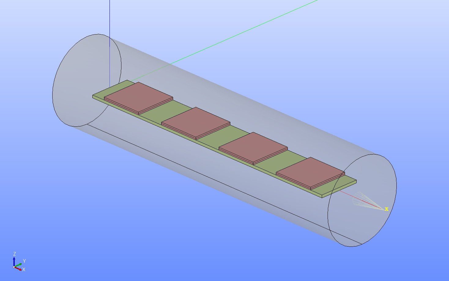
Figure 2: CAD model of the piezoelectric fan: on the epoxy beam (green), four piezoelectric patches (red) are attached comprising the continuum body ${\mathcal{B}_{0}}$ embedded in air (gray, transparent).

Piezoelectric patches are made of 2 layers each of $0.5$ mm thickness. They are poled along $z$-direction. For the piezoceramic and epoxy, we use the stiffness matrix $C_{IJ}$ in Voigt’s notation

$$\begin{gathered}C_{IJ}=\begin{pmatrix}C_{1111}&C_{1122}&C_{1133}&C_{1123}&C_{1113}&C_{1112}\\ C_{2211}&C_{2222}&C_{2233}&C_{2223}&C_{2213}&C_{2212}\\ C_{3311}&C_{3322}&C_{3333}&C_{3323}&C_{3313}&C_{3312}\\ C_{2311}&C_{2322}&C_{2333}&C_{2323}&C_{2313}&C_{2312}\\ C_{1311}&C_{1322}&C_{1333}&C_{1323}&C_{1313}&C_{1312}\\ C_{1211}&C_{1222}&C_{1233}&C_{1223}&C_{1213}&C_{1212}\end{pmatrix}\ .\end{gathered}$$ (114)

Epoxy is an amorph material having translational and rotational symmetry such that the stiffness matrix is isotropic,

$$\begin{gathered}C_{IJ}=\begin{pmatrix}\lambda+2\mu&\lambda&\lambda&0&0&0\\ \lambda&\lambda+2\mu&\lambda&0&0&0\\ \lambda&\lambda&\lambda+2\mu&0&0&0\\ 0&0&0&\mu&0&0\\ 0&0&0&0&\mu&0\\ 0&0&0&0&0&\mu\end{pmatrix}\ ,\quad\lambda=\frac{(E-2G)G}{3G-E}\ ,\quad\mu=G\ ,\end{gathered}$$ (115)

with Young’s modulus $E$ and shear modulus $G$. As piezoceramic we use PZT-5H poled along $z=x_{3}$. For this anisotropic PZT-5H, the compliance matrix

$$\begin{gathered}S_{IJ}=\begin{pmatrix}S_{11}&-\nu S_{11}&-\nu S_{11}&0&0&0\\ -\nu S_{11}&S_{11}&-\nu S_{11}&0&0&0\\ -\nu S_{11}&-\nu S_{11}&S_{33}&0&0&0\\ 0&0&0&(1+\nu)S_{11}&0&0\\ 0&0&0&0&(1+\nu)S_{11}&0\\ 0&0&0&0&0&(1+\nu)S_{11}\end{pmatrix}\ ,\end{gathered}$$ (116)

is used to obtain the stiffness matrix $C_{IJ}=(S_{JI})^{-1}$. The piezoelectric constants, $\tilde{d}_{iJ}$, read

$$\begin{gathered}\tilde{d}_{iJ}=\begin{pmatrix}\tilde{d}_{111}&\tilde{d}_{122}&\tilde{d}_{133}&\tilde{d}_{123}&\tilde{d}_{131}&\tilde{d}_{112}\\ \tilde{d}_{211}&\tilde{d}_{222}&\tilde{d}_{233}&\tilde{d}_{223}&\tilde{d}_{231}&\tilde{d}_{212}\\ \tilde{d}_{311}&\tilde{d}_{322}&\tilde{d}_{333}&\tilde{d}_{323}&\tilde{d}_{331}&\tilde{d}_{312}\end{pmatrix}=\begin{pmatrix}0&0&0&0&\tilde{d}_{15}&0\\ 0&0&0&\tilde{d}_{15}&0&0\\ \tilde{d}_{31}&\tilde{d}_{31}&\tilde{d}_{33}&0&0&0\end{pmatrix}\ ,\end{gathered}$$ (117)

where Voigt’s notation is applied on the last two indices (mapping to multiplication by the displacement gradient in Voigt’s notation). The susceptibility is given by the relative permittivity values by

$$\begin{gathered}\chi^{\text{\tiny el.}}_{ij}=\begin{pmatrix}\bar{\varepsilon}^{\text{\tiny el.}}_{11}&0&0\\ 0&\bar{\varepsilon}^{\text{\tiny el.}}_{11}&0\\ 0&0&\bar{\varepsilon}^{\text{\tiny el.}}_{33}\end{pmatrix}-\delta_{ij}\ .\end{gathered}$$ (118)

We assume that the material has no piezomagnetic and magnetoelectric coupling, i.e., $\tilde{S}_{ijk}=0$ and $\tilde{R}_{ij}=0$, respectively. We compile all necessary material parameters in Table 3. Thermoelectric constant and electric conductivity is set to zero for the beam and patches.

Table 3: Material constants used in the simulation for the epoxy material, PZT-5H as the piezoceramic, and the surrounding air.

		Epoxy	PZT-5H	Air
Mass density	$\rho$ in kg/m3	2500	7500
Compliance	$S_{11}$ in m2/N		$16.5\cdot 10^{-12}$
	$S_{12}$ in m2/N		$-4.78\cdot 10^{-12}$
	$S_{13}$ in m2/N		$-8.45\cdot 10^{-12}$
	$S_{33}$ in m2/N		$20.7\cdot 10^{-12}$
	$S_{44}$ in m2/N		$43.5\cdot 10^{-12}$
	$S_{66}$ in m2/N		$42.6\cdot 10^{-12}$
Young’s modulus	$E$ in N/m2	$30\cdot 10^{9}$
Poisson’s ratio	$\nu$	$0.4$
Piezoelectric constants	$\tilde{d}_{33}$ in m/V	0	$585\cdot 10^{-12}$
	$\tilde{d}_{31}$ in m/V	0	$-265\cdot 10^{-12}$
	$\tilde{d}_{15}$ in m/V	0	$730\cdot 10^{-12}$
Dielectric constants	$\bar{\varepsilon}^{\text{\tiny el.}}_{33}$	1	3400	1
	$\bar{\varepsilon}^{\text{\tiny el.}}_{11}$	1	3130	1
Specific heat capacity	$c$ in J/(kg K)	800	350
Coefficients of thermal expansion	$\alpha_{33}$ in K-1	$15\cdot 10^{-6}$	$-4\cdot 10^{-6}$
	$\alpha_{11}$ in K-1	$15\cdot 10^{-6}$	$6\cdot 10^{-6}$
Thermal conductivity	$\kappa$ in W/(m K)	1.3	1.1

We apply a sinusoidal electric potential difference on the piezoelectric patches by grounding the bottom and upper faces and changing the middle surface in time. Along the $z$-axis an electric field emerge that leads to a contraction along $x$ as well as $y$-axis because of $\tilde{d}_{31}$. Since the potential difference from the middle to the top layer and from the middle to the bottom layer produces in electric fields that are opposed to other in the each layer, one layer stretches when the other layer contracts. The bending in each patch bends the entire beam as shown in Fig. 3. We have applied a relatively big potential difference (amplitude) of 50 kV in order to generate a big deformation by using only 2 layers of patches.

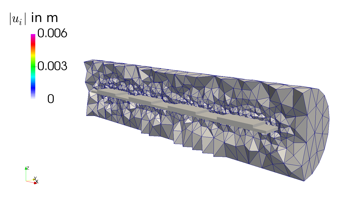
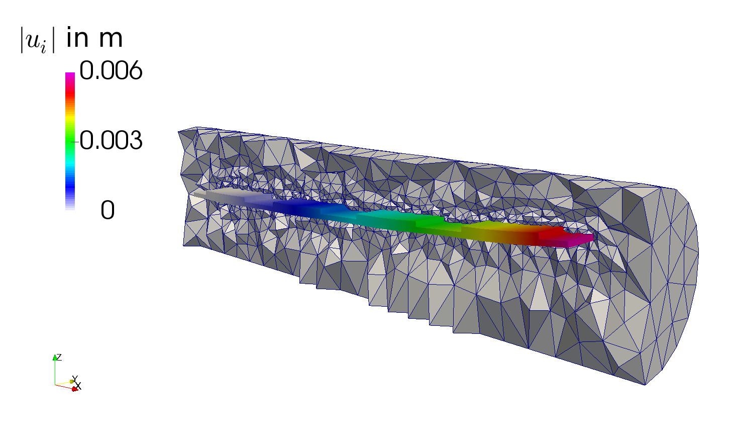
Figure 3: Configuration of the beam bend by the piezoelectric patches. The continuum body is colored by the magnitude of the displacement as well as morphed by the displacement without scaling. The air mesh is not colored and has a crinkle cut to reveal the fan and illustrate the morphing of the elements.

The displacement of the tip and the maximum temperature in the device over the course of the simulation is plotted in Fig. 4. Effected by the exaggerated potential difference, a significant temperature change occurs because of the electric field jump on the middle layer is generated as presented. Further engineering on this type of device would be needed to reduce the required potential difference and resultant heat production, which is possible due to the fully coupled simulation demonstrated.

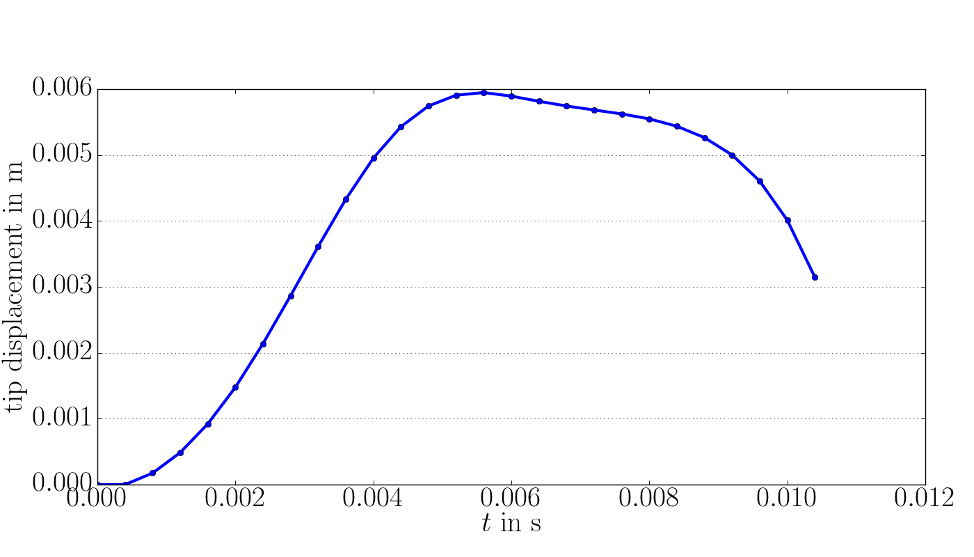
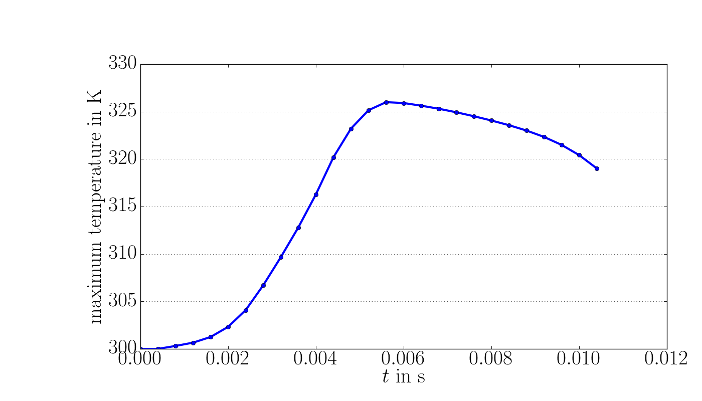
Figure 4: Displacement of the tip of the device (left) and the maximum temperature in the device (right) over the course of the simulation.

5.2 Magnetorheological elastomer

The deformation and magnetic field coupling is often called magnetostriction; but it is insignificant in natural materials. By designing a functionalized material, this behavior is used extensively for smart structures. Consider an elastomer filled with iron spherical particles with sizes on the order of micrometers. To model this material at the macroscopic scale, we homogenize the material into a magnetorheological elastomer. The thermomechanical behavior of the composite will be primarily representative of the elastomer matrix, with additional electromagnetic properties due to the iron additives. Because the iron particles are spherical, an elastomer with an amorph structure will remain isotropic if no external magnetic field was applied during the curing, see Li et al. (2013). This crystalline structure with inversion symmetry prohibits any piezoelectric effects, $\tilde{T}_{ijk}=0$. We assume that the magnetoelectric coupling vanishes, $\tilde{R}_{ij}=0$. A piezoelectric effect is possible depending on the crosslinking of the polymer chains in the elastomer. A magnetoelectric coupling is also expected to arise as a consequence of this effect. The computational framework could include this effect with the necessary material constants, but it was neglected for this simulation.

The functionalized material considered is taken to be a silicone gel TSE2062 filled with carbonyl-iron particles. By assuming an equal and distinct distribution and successful curing, the elastomer has the thermomechanical properties of the silicon. This approximation depends on the relative amount of the iron particles used in the manufacturing. Increasing the amount leads to agglomerated particles building “bridges” between the distinct iron particles such that the thermomechanical characteristics of the composite material change dramatically. For an accurate treatment we refer to Zohdi and Wriggers (2008) and Zohdi (2012). The material properties of the composite material—the particles embedded within the gel—are challenging to quantify, see the measurements in Jolly et al. (1996); An et al. (2012); Yu et al. (2017). Accurate material modeling of these measurements is also discussed heavily in the literature Brigadnov and Dorfmann (2003); Kankanala and Triantafyllidis (2004); Saxena et al. (2014); Spieler et al. (2014); Sutrisno et al. (2015); Metsch et al. (2016); Schubert and Harrison (2016); Mehnert et al. (2017); Cantera et al. (2017).

The following free energy density is the basis of modeling materials response by using the deformation gradient, $\bm{F}$ and the magnetic flux density, $\bm{B}$, as follows:

$$\begin{gathered}\rho_{0}\mathscr{f}=\frac{\mu}{4}\bigg{(}1+\tilde{\alpha}\tanh\Big{(}\frac{I_{4}}{B_{\text{s}}}\Big{)}\bigg{)}\Big{(}(1+n)(I_{1}-3)+(1-n)(I_{2}-3)\Big{)}+qI_{4}+rI_{6}\ ,\\ C_{ij}=F_{ji}F_{jk}\ ,\quad I_{1}=C_{ii}\ ,\quad I_{2}=\frac{1}{2}\Big{(}I_{1}^{2}-C_{ij}C_{ji}\Big{)}\ ,\quad I_{4}=B_{i}B_{i}\ ,\quad I_{6}=C_{ij}B_{j}C_{ik}B_{k}\ .\end{gathered}$$ (119)

We have assumed an isochoric material as well as a neo-Hookean mechanical response. The parameters used for composite material are

$$\begin{gathered}\mu=260\cdot 10^{3}\,\text{Pa}\ ,\quad B_{\text{s}}=1\,\text{T}^{2}\ ,\quad\tilde{\alpha}=0.3\ ,\quad n=0.3\ ,\quad q=r=\frac{1}{\mu_{0}}\ .\end{gathered}$$ (120)

A simple plate of 10 mm$\times$10 mm$\times$1 mm is embedded in air as shown in Fig. 5.

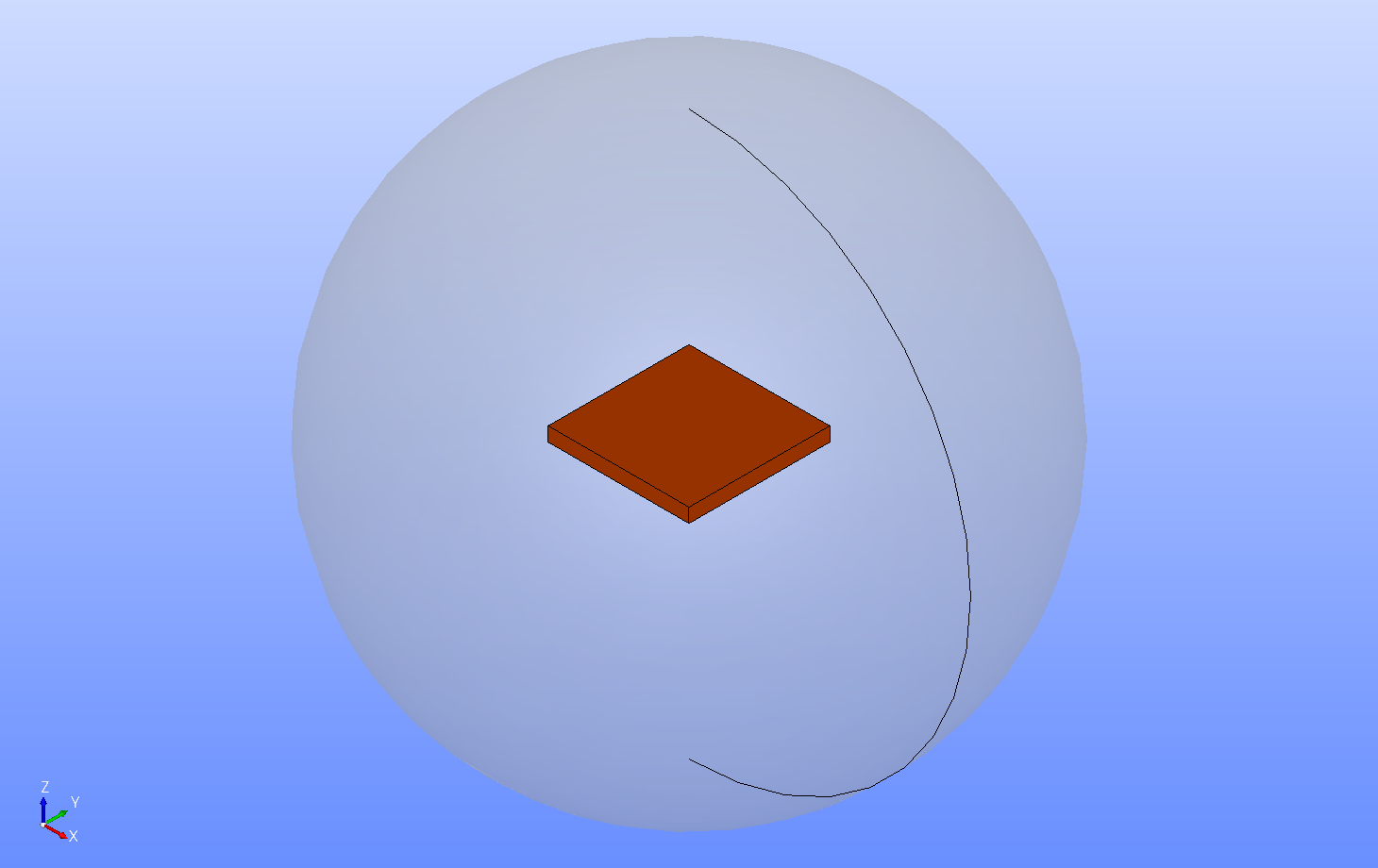
Figure 5: CAD model of the magnetorheological elastomer (orange) embedded in air (gray, transparent).

The plate is clamped on one side and a tangential traction is applied to opposite end oriented in the $z$-axis. We first apply the load with no electromagnetic fields present, deforming it from its reference state into to an initial, deformed state shown in Fig. 6. This step is performed as a nonlinear static solution of only the mechanical fields.

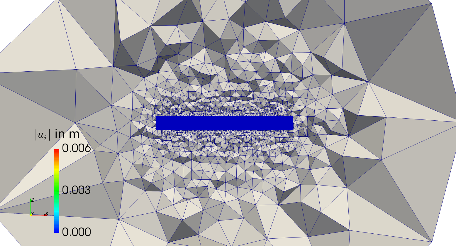
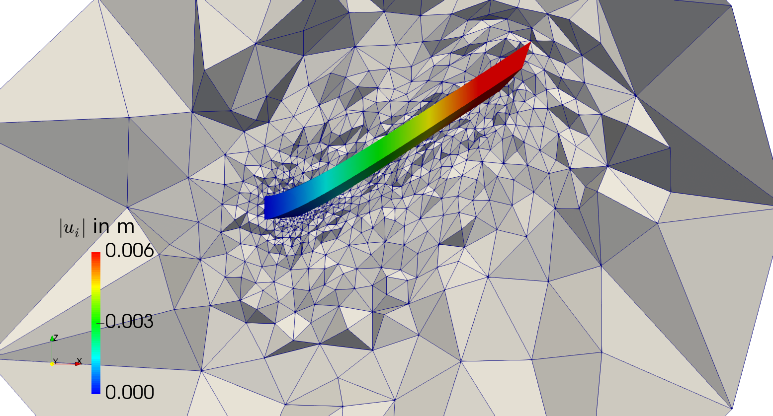
Figure 6: Configuration of the magnetorheological elastomer before and after the mechanical load is applied. The plate is colored by the magnitude of the displacement as well as morphed by the displacement without scaling. The air or vacuum mesh is not colored by any field and has a crinkle cut to present the morphing of the elements.

We emphasize that no scaling is used such that the presented deformation is the actual computed deformation. The mechanical load is held constant throughout the rest of simulation. At the outer boundaries, $\partial\Omega$, the following magnetic potential is applied leading to a time-varying spatially-constant magnetic flux,

$$\begin{gathered}A_{i}=\begin{pmatrix}0\\ xB_{\text{o}}\sin(2\uppi\nu t)\\ 0\end{pmatrix}\ ,\quad B_{i}=\epsilon_{ijk}\frac{\partial A_{k}}{\partial x_{j}}=\begin{pmatrix}0\\ 0\\ B_{\text{o}}\sin(2\uppi\nu t)\end{pmatrix}\ ,\quad\forall\bm{x}\in\partial\Omega\ .\end{gathered}$$ (121)

The boundary conditions are $\phi=0$ and the above form for $\bm{A}$ using a period of 10 s, meaning $\nu=0.1$. The deformation change at 3 s and 6 s is presented in Fig. 7.

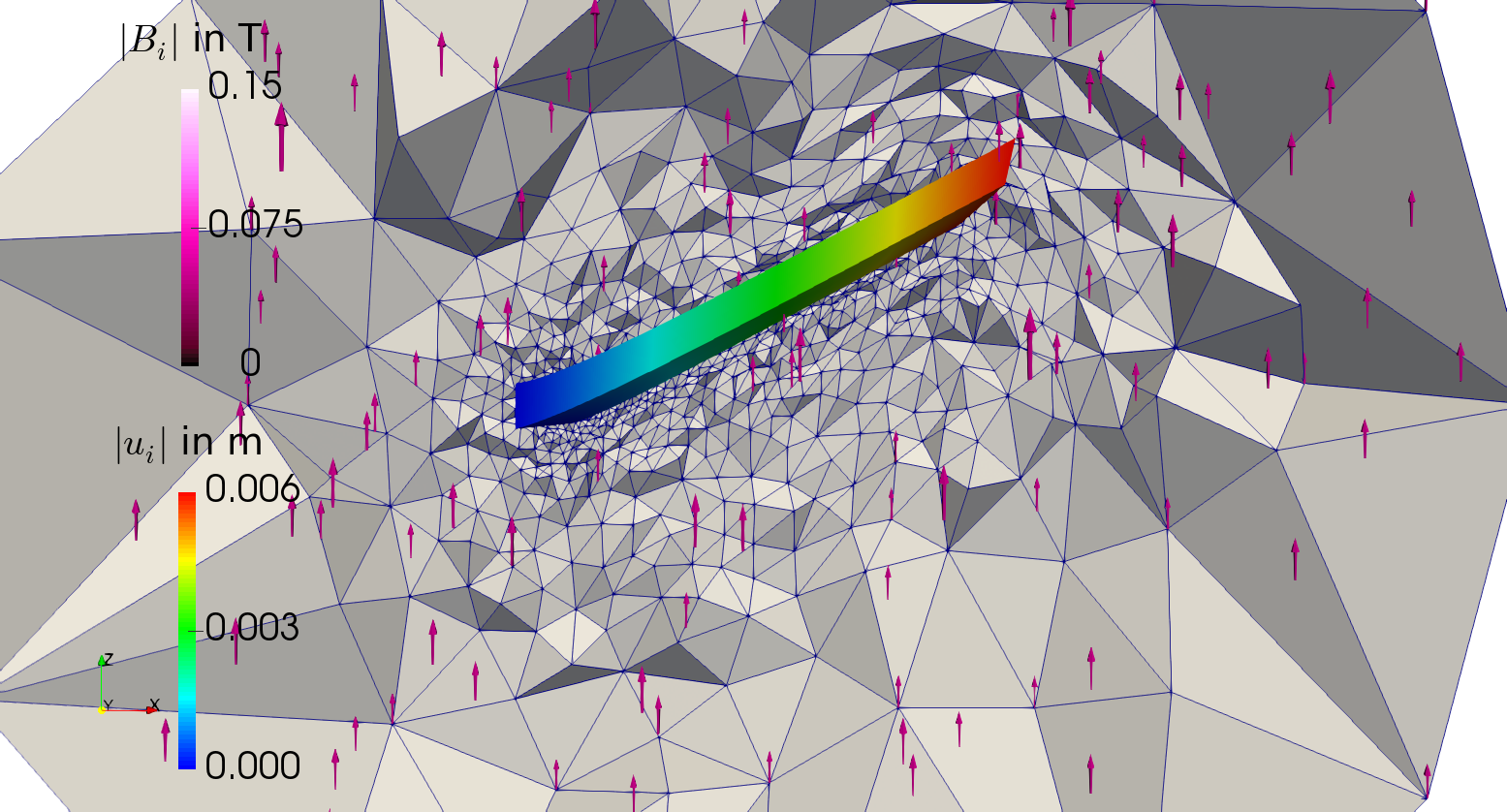
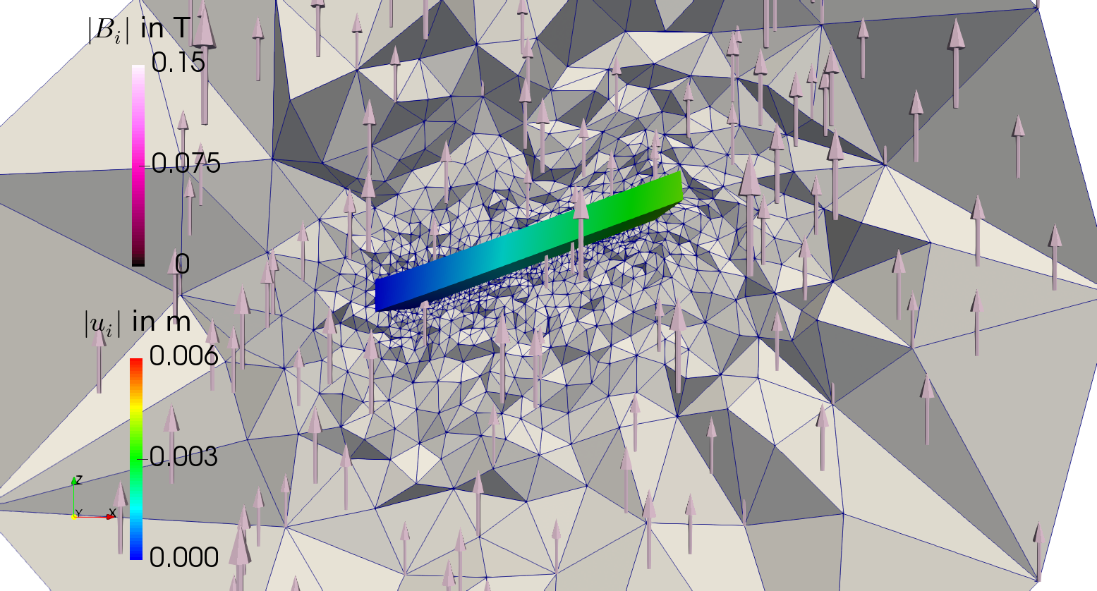
Figure 7: Configuration of the magnetorheological elastomer as the magnetic field is increased as 3 s (left) and 6 s (right). The arrows indicated the magnitude and orientation of the magnetic flux density $B$. The plate is colored by the magnitude of the displacement as well as morphed by the displacement without scaling. The air or vacuum mesh is not colored by any field and has a crinkle cut to present the morphing of the elements.

As the magnetic field increases, the body effectively stiffens leading to a smaller deformation under the same applied force. The stiffening of the structure is controlled by the material parameters in Eq. (119), mainly by $\tilde{\alpha}$ until the saturation is achieved at $B_{\text{s}}$. As seen in Fig. 7, increasing $\bm{B}$ increases the stiffening effect, decreasing the magnitude of the deformation. This contactless stiffening mechanism could be used as either a sensor or actuator in a power transmission application where a winding (not included in the simulation) would be used to generate or sense the magnetic field.

5.3 Thermoelectric heat recovery

We demonstrate the applicability of the our computational framework by simulating a thermoelectric energy recovery system suitable for use in computing servers (clusters). Especially in parallel computing, hundreds of CPUs work collectively and a significant amount of energy is dissipated from the CPUs. By using the thermoelectric effects, part of the dissipating energy can be recovered. The device is an assembly of two integrated circuits joined by copper traces, and a thermoelectric ceramic mounted on top of a substrate. The whole assembly is over-molded in a silicon gel in order to reduce the environmental effects like corrosion. The device is shown in Fig 8, left is the electronic part and right is the mold cutting the contact of electronic parts with the environment. An alternating current (AC) is used with an electric potential difference of 12 V on the trace endings in front as seen in Fig. 8. During operation, Joule heating causes a temperature increase on the microchip leading to an electric current across the piezoceramic sheet measured as a potential difference. This sheet includes an assembly of conductive materials with a thermoelectric constant $\pi$ generating an electric current in Eq. (92) because of a temperature difference. Even in this very simple model, there are different materials and several interfaces. The board is a composite material, mostly it is made of glass reinforced epoxy resin. The microchips are represented as ceramic materials without the detailed internal assembly. Copper traces are used.

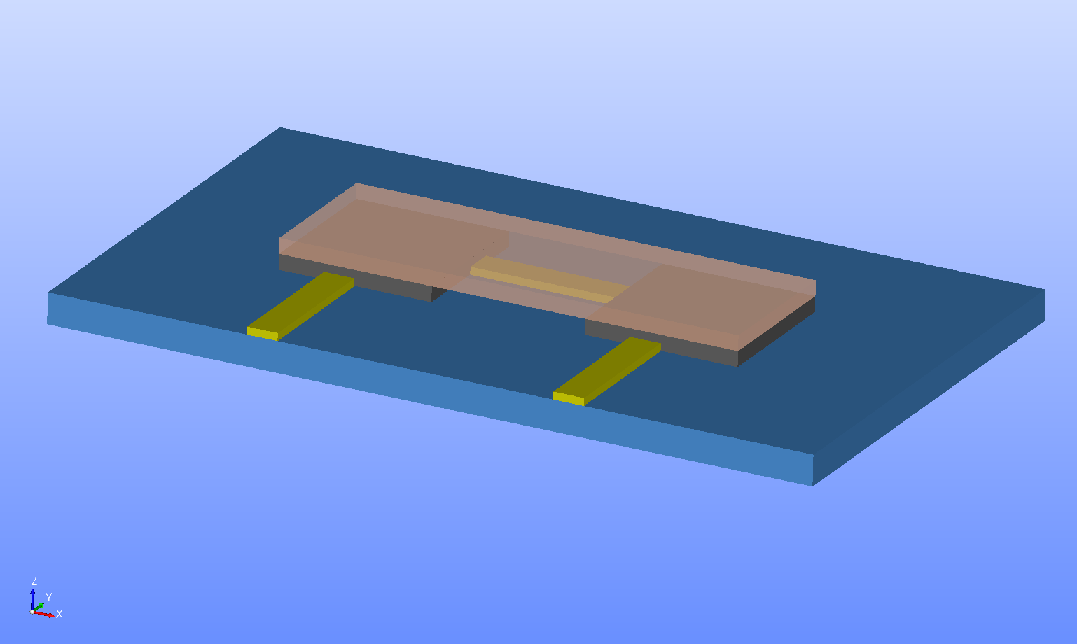
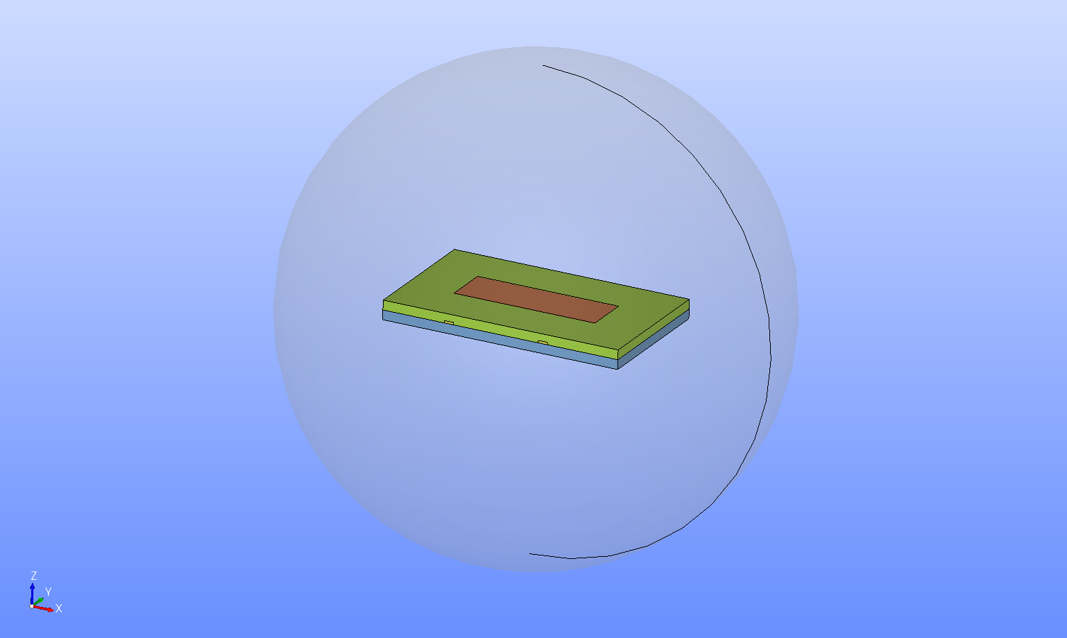
Figure 8: A simplified circuit board. Left: On the board (blue) two microchips (gray) are attached that are connected by traces (yellow). On top of the chips a thermoelectric ceramic (transparent, orange) is placed. Right: The whole assembly out of the board, chips, traces overmolded by a silicon gel (green) is embedded in air (transparent, gray).

An electric potential difference is imposed at the endpoints of traces in front side of the device (apparent in Fig. 8 (left)) by using Dirichlet boundary conditions. This difference creates an electric current through the microchips leading to Joule’s heating. As a result, the microchips heat up the thermoelectric ceramic sheet from below, at the same time, on top of the sheet a cooling agent (like water in a closed system) reduces the temperature by a mixed boundary condition, $h(T-T_{\ref{)}}$, simulated with a high convection constant $h=10^{5}$ J/(s m² K). The temperature difference over the thermoelectric sheet generates a heat flux and an electric current, which results in an electric potential difference across the top and bottom layers of the thermoelectric sheet. We record this induced difference over time and present in Fig. 9.

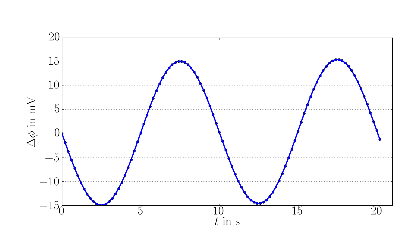
Figure 9: Output of the thermoelectric device, electric potential difference, $\Delta\phi$ in mV, as a result of AC put over the traces.

The thermoelectric energy harvesting shown in this simulation is not very effective; however, it can be used in clusters just to recover a small fraction of the dissipating energy. We stress that this coupling is inherent in the material and no degradation is expected to occur. Hence, it is potentially of interest to use the initial investment to enable energy recovery over the total service life of the cluster.

6 Conclusion

We have developed a complete theory of continuum mechanics with electromagnetic interaction in solid bodies under large deformations. Balance equations for mechanical, thermal, and electromagnetic fields have been discussed and all necessary constitutive equations have been derived by exploiting thermodynamical principles. The constitutive equations are general and involve all coupling phenomena resulting in piezoelectric, pyroelectric, and thermoelectric responses. Some irreversible effects are neglected, such as plasticity, viscoelasticity, and material hysteresis with respect to the electromagnetic fields. The proposed approach is general for polarized elastic materials subject to large deformations. The formulation results in a nonlinear variational form with complete coupling of all of the mechanical and electromagnetic fields. In order to reduce the computational cost, we have proposed a novel method and solve electromagnetic fields in the whole domain, whereas the deformation and temperature are solved only within the continuum body. Separation of field and matter is possible; however, their equations are defined in different placements. Therefore, from the very beginning of the development of the theory, we have emphasized different frames by using an explicit notation. Numerical solution is possible in the Lagrangean and Eulerian frames by using a staggered scheme with an appropriate mesh morphing algorithm. The nonlinear variational forms have been solved for thermomechanical and electromagnetic fields by using the finite element method with the aid of open-source packages developed under the FEniCS project. In order to encourage further achievements, the mesh morphing algorithm implementation is released under the GNU LGPL https://github.com/afqueiruga/afqsfenicsutil and the scripts and geometry files that performed the simulations are released under the GNU GPL at the repository https://github.com/afqueiruga/EMSI-2018.

References

Appendix A Electric current due to the bound charges

By using

$$\begin{gathered}D_{i}=\mathfrak{D}_{i}-P_{i}\ ,\quad H_{i}=\mathfrak{H}_{i}+\mathscr{M}_{i}\end{gathered}$$ (122)

in Maxwell’s equations

$$\begin{gathered}\frac{\partial\mathfrak{D}_{i}}{\partial x_{i}}-\frac{\partial P_{i}}{\partial x_{i}}=\rho z^{\text{fr.}}+\rho z^{\text{bo.}}\ ,\\ -\frac{\partial\mathfrak{D}_{i}}{\partial t}+\frac{\partial P_{i}}{\partial t}+\epsilon_{ijk}\frac{\partial\mathfrak{H}_{k}}{\partial x_{j}}+\epsilon_{ijk}\frac{\partial\mathscr{M}_{k}}{\partial x_{j}}=J_{i}\ ,\end{gathered}$$ (123)

we realize

$$\begin{gathered}\frac{\partial\mathfrak{D}_{i}}{\partial x_{i}}=\rho z^{\text{fr.}}\ ,\quad-\frac{\partial P_{i}}{\partial x_{i}}=\rho z^{\text{bo.}}\ ,\\ -\frac{\partial\mathfrak{D}_{i}}{\partial t}+\epsilon_{ijk}\frac{\partial\mathfrak{H}_{k}}{\partial x_{j}}=J_{i}-\frac{\partial P_{i}}{\partial t}-\epsilon_{ijk}\frac{\partial\mathscr{M}_{k}}{\partial x_{j}}=J_{i}^{\text{fr.}}\ .\end{gathered}$$ (124)

Appendix B Balance of electromagnetic momentum

We start by obtaining the time rate of the chosen electromagnetic momentum

$$\begin{gathered}\frac{\partial\mathscr{G}_{i}}{\partial t}=\frac{\partial\epsilon_{ijk}\mathfrak{D}_{j}B_{k}}{\partial t}=\epsilon_{ijk}\frac{\partial D_{j}B_{k}}{\partial t}+\epsilon_{ijk}\frac{\partial P_{j}B_{k}}{\partial t}\ .\end{gathered}$$ (125)

The first term can be rewritten, by using

$$\begin{gathered}\epsilon_{ijk}=-\epsilon_{ikj}\ ,\quad\epsilon_{ijk}\epsilon_{klm}=\delta_{il}\delta_{jm}-\delta_{im}\delta_{jl}\ ,\end{gathered}$$ (126)

as well as Maxwell’s equations

$$\begin{gathered}\epsilon_{ijk}\frac{\partial D_{j}B_{k}}{\partial t}=\epsilon_{ijk}\Big{(}\epsilon_{jlm}\frac{\partial H_{m}}{\partial x_{l}}-J_{j}\Big{)}B_{k}-\epsilon_{ijk}D_{j}\epsilon_{klm}\frac{\partial E_{m}}{\partial x_{l}}=\\ =-\frac{\partial H_{k}}{\partial x_{i}}B_{k}+\frac{\partial H_{i}}{\partial x_{k}}B_{k}-(\bm{J}\times\bm{B})_{i}-D_{j}\frac{\partial E_{j}}{\partial x_{i}}+D_{j}\frac{\partial E_{i}}{\partial x_{j}}\ .\end{gathered}$$ (127)

Moreover, by using Maxwell–Lorentz aether relations we observe

$$\begin{gathered}\frac{\partial H_{k}}{\partial x_{i}}B_{k}=\frac{1}{\mu_{0}}\frac{\partial B_{k}}{\partial x_{i}}B_{k}=\frac{1}{\mu_{0}}\frac{\partial}{\partial x_{i}}\Big{(}\frac{1}{2}B_{k}B_{k}\Big{)}=\frac{1}{2}\frac{\partial H_{k}B_{k}}{\partial x_{i}}\ ,\\ D_{j}\frac{\partial E_{j}}{\partial x_{i}}=\varepsilon_{0}E_{j}\frac{\partial E_{j}}{\partial x_{i}}=\varepsilon_{0}\frac{\partial}{\partial x_{i}}\Big{(}\frac{1}{2}E_{j}E_{j}\Big{)}=\frac{1}{2}\frac{\partial D_{j}E_{j}}{\partial x_{i}}\ .\end{gathered}$$ (128)

Finally, by utilizing Maxwell’s equations we achieve

$$\begin{gathered}\frac{\partial H_{i}}{\partial x_{k}}B_{k}=\frac{\partial H_{i}B_{k}}{\partial x_{k}}\ ,\\ D_{j}\frac{\partial E_{i}}{\partial x_{j}}=\frac{\partial D_{j}E_{i}}{\partial x_{j}}-\rho zE_{i}\ .\end{gathered}$$ (129)

By combining all above, we obtain

$$\begin{gathered}\frac{\partial\mathscr{G}_{i}}{\partial t}=\frac{\partial}{\partial x_{j}}\underbrace{\Big{(}-\frac{1}{2}\delta_{ij}\big{(}D_{k}E_{k}+H_{k}B_{k}\big{)}+H_{i}B_{j}+D_{j}E_{i}\Big{)}}_{m_{ji}}-\underbrace{\Big{(}\rho zE_{i}+(\bm{J}\times\bm{B})_{i}-\frac{\partial(\bm{P}\times\bm{B})_{i}}{\partial t}\Big{)}}_{\mathscr{F}_{i}}\ ,\end{gathered}$$ (130)

after comparing to the the balance of electromagnetic momentum.

Appendix C Balance of electromagnetic energy

By starting with the divergence of the chosen electromagnetic flux

$$\begin{gathered}\frac{\partial\mathscr{P}_{i}}{\partial x_{i}}=\epsilon_{ijk}\frac{\partial\mathfrak{H}_{j}E_{k}}{\partial x_{i}}=\epsilon_{ijk}\frac{\partial H_{j}E_{k}}{\partial x_{i}}-\underbrace{\epsilon_{ijk}\frac{\partial\mathscr{M}_{j}E_{k}}{\partial x_{i}}}_{\displaystyle\frac{\partial(\boldsymbol{\mathscr{M}}\times\bm{E})_{i}}{\partial x_{i}}}\ ,\end{gathered}$$ (131)

we can rewrite the first term by using $\epsilon_{ijk}=\epsilon_{jki}=\epsilon_{kij}$ and $\epsilon_{ijk}=-\epsilon_{jik}$, as well as inserting Maxwell’s equations,

$$\begin{gathered}\epsilon_{ijk}\frac{\partial H_{j}E_{k}}{\partial x_{i}}=\epsilon_{kij}\frac{\partial H_{j}}{\partial x_{i}}E_{k}-H_{j}\epsilon_{jik}\frac{\partial E_{k}}{\partial x_{i}}=\Big{(}\frac{\partial D_{k}}{\partial t}+J_{k}\Big{)}E_{k}+H_{j}\frac{\partial B_{j}}{\partial t}=\\ =\frac{\partial}{\partial t}\Big{(}\frac{1}{2}D_{k}E_{k}+\frac{1}{2}H_{j}B_{j}\Big{)}+J_{k}E_{k}\ .\end{gathered}$$ (132)

Since we have

$$\begin{gathered}J_{i}E_{i}=\Big{(}J_{i}^{\text{fr.}}+\frac{\partial P_{i}}{\partial t}+\epsilon_{ijk}\frac{\partial\mathscr{M}_{k}}{\partial x_{j}}\Big{)}E_{i}=J_{i}^{\text{fr.}}E_{i}+\frac{\partial P_{i}E_{i}}{\partial t}-P_{i}\frac{\partial E_{i}}{\partial t}+\epsilon_{ijk}\frac{\partial\mathscr{M}_{k}E_{i}}{\partial x_{j}}-\mathscr{M}_{k}\epsilon_{ijk}\frac{\partial E_{i}}{\partial x_{j}}=\\ =J_{i}^{\text{fr.}}E_{i}+\frac{\partial P_{i}E_{i}}{\partial t}-P_{i}\frac{\partial E_{i}}{\partial t}+\epsilon_{jki}\frac{\partial\mathscr{M}_{k}E_{i}}{\partial x_{j}}+\mathscr{M}_{k}\epsilon_{kji}\frac{\partial E_{i}}{\partial x_{j}}=\\ =J_{i}^{\text{fr.}}E_{i}+\frac{\partial P_{i}E_{i}}{\partial t}-P_{i}\frac{\partial E_{i}}{\partial t}+\frac{\partial(\boldsymbol{\mathscr{M}}\times\bm{E})_{j}}{\partial x_{j}}-\mathscr{M}_{k}\frac{\partial B_{k}}{\partial t}=\\ =J_{i}^{\text{fr.}}E_{i}+\frac{\partial}{\partial t}(P_{i}E_{i}-\mathscr{M}_{i}B_{i})-P_{i}\frac{\partial E_{i}}{\partial t}+\frac{\partial(\boldsymbol{\mathscr{M}}\times\bm{E})_{j}}{\partial x_{j}}+B_{k}\frac{\partial\mathscr{M}_{k}}{\partial t}\ ,\end{gathered}$$ (133)

we obtain

$$\begin{gathered}\frac{\partial\mathscr{P}_{i}}{\partial x_{i}}=\frac{\partial}{\partial t}\Big{(}P_{i}E_{i}-\mathscr{M}_{i}B_{i}+\frac{1}{2}(D_{k}E_{k}+H_{j}B_{j})\Big{)}+J_{i}^{\text{fr.}}E_{i}-P_{i}\frac{\partial E_{i}}{\partial t}+B_{k}\frac{\partial\mathscr{M}_{k}}{\partial t}\ ,\\ \frac{\partial}{\partial t}\underbrace{\Big{(}P_{i}E_{i}-\mathscr{M}_{i}B_{i}+\frac{1}{2}(D_{k}E_{k}+H_{j}B_{j})\Big{)}}_{\displaystyle e^{\text{\tiny f.}}}=\frac{\partial\mathscr{P}_{i}}{\partial x_{i}}-\underbrace{\Big{(}J_{i}^{\text{fr.}}E_{i}-P_{i}\frac{\partial E_{i}}{\partial t}+B_{k}\frac{\partial\mathscr{M}_{k}}{\partial t}\Big{)}}_{\displaystyle\pi}\ ,\end{gathered}$$ (134)

Appendix D Maxwell symmetry

The Maxwell symmetry relations can be seen by using simple relations,

$$\begin{gathered}\tilde{c}^{21}_{ji}=\frac{\partial n_{ji}}{\partial T}=\frac{\partial^{2}\mathscr{f}}{\partial T\partial F_{ij}}=\frac{\partial^{2}\mathscr{f}}{\partial F_{ij}\partial T}=-\frac{\partial\eta}{\partial F_{ij}}=-\tilde{c}^{12}_{ij}\ ,\\ \tilde{c}^{31}_{i}=\frac{\partial p_{i}}{\partial T}=-\frac{\partial^{2}\mathscr{f}}{\partial T\partial E_{i}}=-\frac{\partial^{2}\mathscr{f}}{\partial E_{i}\partial T}=\frac{\partial\eta}{\partial E_{i}}=\tilde{c}^{13}_{i}\ ,\\ \tilde{c}^{41}_{i}=\frac{\partial\mathscr{m}_{i}}{\partial T}=-\frac{\partial^{2}\mathscr{f}}{\partial T\partial B_{i}}=-\frac{\partial^{2}\mathscr{f}}{\partial B_{i}\partial T}=\frac{\partial\eta}{\partial B_{i}}=\tilde{c}^{14}_{i}\ ,\\ \tilde{c}^{51}=\frac{\partial\mathscr{p}}{\partial T}=-\frac{\partial^{2}\mathscr{f}}{\partial T\partial\mathrm{v}}=-\frac{\partial^{2}\mathscr{f}}{\partial\mathrm{v}\partial T}=\frac{\partial\eta}{\partial\mathrm{v}}=\tilde{c}^{15}\ ,\\ \end{gathered}$$ (135)

furthermore,

$$\begin{gathered}\tilde{c}^{32}_{ikl}=\frac{\partial p_{i}}{\partial F_{kl}}=-\frac{\partial^{2}\mathscr{f}}{\partial F_{kl}\partial E_{i}}=-\frac{\partial^{2}\mathscr{f}}{\partial E_{i}\partial F_{kl}}=-\frac{\partial n_{lk}}{\partial E_{i}}=-\tilde{c}^{23}_{lki}\ ,\\ \tilde{c}^{42}_{ikl}=\frac{\partial\mathscr{m}_{i}}{\partial F_{kl}}=-\frac{\partial^{2}\mathscr{f}}{\partial F_{kl}\partial B_{i}}=-\frac{\partial^{2}\mathscr{f}}{\partial B_{i}\partial F_{kl}}=-\frac{\partial n_{lk}}{\partial B_{i}}=-\tilde{c}^{24}_{lki}\ ,\\ \tilde{c}^{52}_{kl}=\frac{\partial\mathscr{p}}{\partial F_{kl}}=-\frac{\partial^{2}\mathscr{f}}{\partial F_{kl}\partial\mathrm{v}}=-\frac{\partial^{2}\mathscr{f}}{\partial\mathrm{v}\partial F_{kl}}=-\frac{\partial n_{lk}}{\partial\mathrm{v}}=-\tilde{c}^{25}_{lk}\ ,\end{gathered}$$ (136)

as well as

$$\begin{gathered}\tilde{c}^{43}_{ik}=\frac{\partial\mathscr{m}_{i}}{\partial E_{k}}=-\frac{\partial^{2}\mathscr{f}}{\partial E_{k}\partial B_{i}}=-\frac{\partial^{2}\mathscr{f}}{\partial B_{i}\partial E_{k}}=\frac{\partial p_{k}}{\partial B_{i}}=\tilde{c}^{34}_{ki}\ ,\\ \tilde{c}^{53}_{k}=\frac{\partial\mathscr{p}}{\partial E_{k}}=-\frac{\partial^{2}\mathscr{f}}{\partial E_{k}\partial\mathrm{v}}=-\frac{\partial^{2}\mathscr{f}}{\partial\mathrm{v}\partial E_{k}}=\frac{\partial p_{k}}{\partial\mathrm{v}}=\tilde{c}^{35}_{k}\ ,\end{gathered}$$ (137)

and

$$\begin{gathered}\tilde{c}^{54}_{k}=\frac{\partial\mathscr{p}}{\partial B_{k}}=-\frac{\partial^{2}\mathscr{f}}{\partial B_{k}\partial\mathrm{v}}=-\frac{\partial^{2}\mathscr{f}}{\partial\mathrm{v}\partial B_{k}}=\frac{\partial\mathscr{m}_{k}}{\partial\mathrm{v}}=\tilde{c}^{45}_{k}\ .\end{gathered}$$ (138)

References

- Abali (2016) B. E. Abali. Computational Reality, Solving Nonlinear and Coupled Problems in Continuum Mechanics. Advanced Structured Materials. Springer, 2016. ISBN 978-981-10-2443-6.
- Abali and Reich (2017) B. E. Abali and F. A. Reich. Thermodynamically consistent derivation and computation of electro-thermo-mechanical systems for solid bodies. Computer Methods in Applied Mechanics and Engineering, 2017.
- Abali and Reich (2018) B. E. Abali and F. A. Reich. Verification of deforming polarized structure computation by using a closed-form solution. Continuum Mechanics and Thermodynamics, pages 1–16, 2018. ISSN 0935-1175. URL https://doi.org/10.1007/s00161-018-0709-8.
- Abali et al. (2017) B. E. Abali, W. H. Müller, and F. dell’Isola. Theory and computation of higher gradient elasticity theories based on action principles. Archive of Applied Mechanics, 87(9):1495–1510, 2017.
- Ahmad et al. (2006) S. N. Ahmad, C. S. Upadhyay, and C. Venkatesan. Electro-thermo-elastic formulation for the analysis of smart structures. Smart materials and structures, 15(2):401, 2006.
- Altenbach et al. (2013) H. Altenbach, S. Forest, and A. Krivtsov. Generalized continua as models for materials. With Multi-scale Effects or Under Multifield Actions,-Springer, New York, 2013.
- An et al. (2012) H. An, S. J. Picken, and E. Mendes. Nonlinear rheological study of magneto responsive soft gels. Polymer, 53(19):4164–4170, 2012.
- Arnold and Logg (2014) D. N. Arnold and A. Logg. Periodic table of the finite elements. SIAM News, 47(9), 2014.
- Assous et al. (2017) F. Assous, P. Ciarlet, and S. Labrunie. Mathematical foundations of computational electromagnetism. Springer, 2017.
- Ausanio et al. (2005) G. Ausanio, A. C. Barone, C. Hison, V. Iannotti, G. Mannara, and L. Lanotte. Magnetoelastic sensor application in civil buildings monitoring. Sensors and Actuators A: Physical, 123:290–295, 2005.
- Barham et al. (2010) M. I. Barham, D. A. White, and D. J. Steigmann. Finite element modeling of the deformation of magnetoelastic film. Journal of Computational Physics, 229(18):6193–6207, 2010.
- Barnett (2010) S. M. Barnett. Resolution of the Abraham–Minkowski dilemma. Physical Review Letters, 104(7):070401, 2010.
- Bastos and Sadowski (2003) J. P. A. Bastos and N. Sadowski. Electromagnetic modeling by finite element methods. CRC press, 2003.
- Baumanns et al. (2013) S. Baumanns, M. Clemens, and S. Schops. Structural aspects of regularized full maxwell electrodynamic potential formulations using fit. In Electromagnetic Theory (EMTS), Proceedings of 2013 URSI International Symposium on, pages 1007–1010. IEEE, 2013.
- Benjeddou (2000) A. Benjeddou. Advances in piezoelectric finite element modeling of adaptive structural elements: a survey. Computers & Structures, 76(1):347–363, 2000.
- Bethune-Waddell and Chau (2015) M. Bethune-Waddell and K. J. Chau. Simulations of radiation pressure experiments narrow down the energy and momentum of light in matter. Reports on Progress in Physics, 78(12):122401, 2015.
- Bieńkowski et al. (2010) A. Bieńkowski, R. Szewczyk, and J. Salach. Industrial application of magnetoelastic force and torque sensors. Acta Physica Polonica A, 118(5):1008–1009, 2010.
- Bossavit (1988) A. Bossavit. Whitney forms: A class of finite elements for three-dimensional computations in electromagnetism. IEE Proceedings A (Physical Science, Measurement and Instrumentation, Management and Education, Reviews), 135(8):493–500, 1988.
- Brechet and Ansermet (2014) S. D. Brechet and J.-P. Ansermet. Thermodynamics of continuous media with intrinsic rotation and magnetoelectric coupling. Continuum Mechanics and Thermodynamics, 26(2):115–142, 2014.
- Brigadnov and Dorfmann (2003) I. A. Brigadnov and A. Dorfmann. Mathematical modeling of magneto-sensitive elastomers. International Journal of Solids and Structures, 40(18):4659–4674, 2003.
- Brunner et al. (2009) A. J. Brunner, M. Birchmeier, M. M. Melnykowycz, and M. Barbezat. Piezoelectric fiber composites as sensor elements for structural health monitoring and adaptive material systems. Journal of Intelligent Material Systems and Structures, 20(9):1045–1055, 2009.
- Cammarata (1994) R. C. Cammarata. Surface and interface stress effects in thin films. Progress in surface science, 46(1):1–38, 1994.
- Cantera et al. (2017) M. A. Cantera, M. Behrooz, R. F. Gibson, and F. Gordaninejad. Modeling of magneto-mechanical response of magnetorheological elastomers (mre) and mre-based systems: a review. Smart Materials and Structures, 26(2):023001, 2017.
- Caratheodory (1909) C. Caratheodory. Untersuchungen über die Grundlagen der Thermodynamik. Mathematische Annalen, 67(3):355–386, 1909. URL http://dx.doi.org/10.1007/BF01450409.
- Chróścielewski et al. (2018) J. Chróścielewski, R. Schmidt, and V. A. Eremeyev. Nonlinear finite element modeling of vibration control of plane rod-type structural members with integrated piezoelectric patches. Continuum Mechanics and Thermodynamics, pages 1–42, 2018.
- Chu et al. (1966) L. J. Chu, H. A. Haus, and P. Penfield Jr. The force density in polarizable and magnetizable fluids. Proceedings of the IEEE, 54(7):920–935, 1966.
- Chung et al. (2014) Y. Chung, J.-S. Son, T. J. Lee, H. J. Kim, and C. Shin. Three-dimensional modelling of controlled-source electromagnetic surveys using an edge finite-element method with a direct solver. Geophysical Prospecting, 62(6):1468–1483, 2014.
- Ciarlet Jr and Zou (1999) P. Ciarlet Jr and J. Zou. Fully discrete finite element approaches for time-dependent maxwell’s equations. Numerische Mathematik, 82(2):193–219, 1999.
- de Groot and Mazur (1984) S. R. de Groot and P. Mazur. Non-equilibrium thermodynamics, 1984.
- Demkowicz (2006) L. Demkowicz. Computing with hp-adaptive finite elements: volume 1 one and two dimensional elliptic and Maxwell problems. CRC Press, 2006.
- Demkowicz (2017) L. Demkowicz. Finite element methods for maxwell’s equations. Encyclopedia of Computational Mechanics Second Edition, pages 1–20, 2017.
- Dorfmann and Ogden (2017) L. Dorfmann and R. W. Ogden. Nonlinear electroelasticity: material properties, continuum theory and applications. Proceedings of the Royal Society A: Mathematical, Physical and Engineering Sciences, 473(2204):20170311, 2017.
- Ericksen (2007) J. L. Ericksen. On formulating and assessing continuum theories of electromagnetic fields in elastic materials. Journal of Elasticity, 87(2-3):95–108, 2007.
- Eringen and Maugin (1990) A. C. Eringen and G. A. Maugin. Electrodynamics of Continua I: Foundations and Solid Media. Springer, 1990.
- Ethiraj and Miehe (2016) G. Ethiraj and C. Miehe. Multiplicative magneto-elasticity of magnetosensitive polymers incorporating micromechanically-based network kernels. International Journal of Engineering Science, 102:93–119, 2016.
- Frommberger et al. (2003) M. Frommberger, C. Zanke, A. Ludwig, M. Tewes, and E. Quandt. Processing and application of magnetoelastic thin films in high-frequency devices. Microelectronic engineering, 67:588–594, 2003.
- Gibson (2007) W. C. Gibson. The method of moments in electromagnetics. Chapman and Hall/CRC, 2007.
- Gil and Ortigosa (2016) A. J. Gil and R. Ortigosa. A new framework for large strain electromechanics based on convex multi-variable strain energies: Variational formulation and material characterisation. Computer Methods in Applied Mechanics and Engineering, 302:293–328, 2016.
- Gillette et al. (2016) A. Gillette, A. Rand, and C. Bajaj. Construction of scalar and vector finite element families on polygonal and polyhedral meshes. Computational Methods in Applied Mathematics, 16(4):667–683, 2016.
- Ginder et al. (1999) J. M. Ginder, M. E. Nichols, L. D. Elie, and J. L. Tardiff. Magnetorheological elastomers: properties and applications. In Smart Structures and Materials 1999: Smart Materials Technologies, volume 3675, pages 131–139. International Society for Optics and Photonics, 1999.
- Glane et al. (2017) S. Glane, F. A. Reich, and W. H. Müller. Modeling of non-ideal hard permanent magnets with an affine-linear model, illustrated for a bar and a horseshoe magnet. Continuum Mechanics and Thermodynamics, pages 1–21, 2017.
- GNU Public (2007) GNU Public. Gnu general public license. http://www.gnu.org/copyleft/gpl.html, June 2007.
- Griffiths (1999) D. J. Griffiths. Introduction to electrodynamics, volume 3. prentice Hall Upper Saddle River, NJ, 1999.
- Griffiths (2012) D. J. Griffiths. Resource letter em-1: Electromagnetic momentum. American Journal of Physics, 80(1):7–18, 2012.
- Grimes et al. (2011) C. A. Grimes, S. C. Roy, S. Rani, and Q. Cai. Theory, instrumentation and applications of magnetoelastic resonance sensors: a review. Sensors, 11(3):2809–2844, 2011.
- Guo et al. (2017) X. Guo, S. Sang, J. Guo, A. Jian, Q. Duan, J. Ji, Q. Zhang, and W. Zhang. A magnetoelastic biosensor based on e2 glycoprotein for wireless detection of classical swine fever virus e2 antibody. Scientific reports, 7(1):15626, 2017.
- Hachkevych and Terlets’kyi (2004) O. R. Hachkevych and R. F. Terlets’kyi. Models of thermomechanics of magnetizable and polarizable conducting deformable solids. Materials Science, 40(3):320–336, 2004.
- He et al. (2015) W. He, G. Zhang, X. Zhang, J. Ji, G. Li, and X. Zhao. Recent development and application of thermoelectric generator and cooler. Applied Energy, 143:1–25, 2015.
- Hiptmair (2002) R. Hiptmair. Finite elements in computational electromagnetism. Acta Numerica, 11:237–339, 2002.
- Hoffman et al. (2005) J. Hoffman, J. Jansson, C. Johnson, M. Knepley, R. C. Kirby, A. Logg, L. R. Scott, and G. N. Wells. FEniCS. http://www.fenicsproject.org/, 2005.
- Jiang (1998) B. Jiang. The least-squares finite element method: theory and applications in computational fluid dynamics and electromagnetics. Springer Science & Business Media, 1998.
- Jin (2015) J.-M. Jin. The finite element method in electromagnetics. John Wiley & Sons, 2015.
- Jolly et al. (1996) M. R. Jolly, J. D. Carlson, B. C. Muñoz, and T. A. Bullions. The magnetoviscoelastic response of elastomer composites consisting of ferrous particles embedded in a polymer matrix. Journal of Intelligent Material Systems and Structures, 7(6):613–622, 1996.
- Jones (1964) D. S. Jones. The Theory of Electromagnetism. Pergamon, 1964. ISBN 978-0-08-013686-8. doi: http://dx.doi.org/10.1016/B978-0-08-013686-8.50006-X. URL http://www.sciencedirect.com/science/article/pii/B978008013686850006X.
- Jou et al. (1999) D. Jou, J. Casas-Vazquez, and G. Lebon. Extended irreversible thermodynamics revisited (1988-98). Reports on Progress in Physics, 62(7):1035, 1999.
- Kankanala and Triantafyllidis (2004) S. V. Kankanala and N. Triantafyllidis. On finitely strained magnetorheological elastomers. Journal of the Mechanics and Physics of Solids, 52(12):2869–2908, 2004.
- Keip and Schröder (2018) M.-A. Keip and J. Schröder. Multiscale modeling of electroactive polymer composites. In Ferroic Functional Materials, pages 263–285. Springer, 2018.
- Kim and Han (2006) D.-K. Kim and J.-H. Han. Smart flapping wing using macrofiber composite actuators. In Smart Structures and Materials, pages 61730F–61730F. International Society for Optics and Photonics, 2006.
- Klinkel et al. (2013) S. Klinkel, S. Zwecker, and R. Müller. A solid shell finite element formulation for dielectric elastomers. Journal of Applied Mechanics, 80(2):021026, 2013.
- Kodjo et al. (2019) K.-M. Kodjo, J. Yvonnet, M. Karkri, and K. Sab. Multiscale modeling of the thermomechanical behavior in heterogeneous media embedding phase change materials particles. Journal of Computational Physics, 378:303–323, 2019.
- Kovalovs et al. (2007) A. Kovalovs, E. Barkanov, and S. Gluhihs. Active control of structures using macro-fiber composite (mfc). In Journal of Physics: Conference Series, volume 93, page 012034. IOP Publishing, 2007.
- Kovetz (2000) A. Kovetz. Electromagnetic theory. 2000.
- Kraus et al. (2017) M. Kraus, K. Kormann, P. J. Morrison, and E. Sonnendrücker. Gempic: Geometric electromagnetic particle-in-cell methods. Journal of Plasma Physics, 83(4), 2017.
- Lanteri et al. (2018) S. Lanteri, D. Paredes, C. Scheid, and F. Valentin. The multiscale hybrid-mixed method for the maxwell equations in heterogeneous media. Multiscale Modeling & Simulation, 16(4):1648–1683, 2018.
- Lanza-Discalea et al. (2007) F. Lanza-Discalea, H. Matt, I. Bartoli, S. Coccia, G. Park, and C. Farrar. Health monitoring of uav wing skin-to-spar joints using guided waves and macro fiber composite transducers. Journal of intelligent material systems and structures, 18(4):373–388, 2007.
- Li (2009) J. Li. Numerical convergence and physical fidelity analysis for Maxwell’s equations in metamaterials. Computer Methods in Applied Mechanics and Engineering, 198(37):3161–3172, 2009.
- Li et al. (2013) W. H. Li, X. Z. Zhang, and H. Du. Magnetorheological elastomers and their applications. In Advances in Elastomers I, pages 357–374. Springer, 2013.
- Liu and Trung (2016) G.-R. Liu and N. T. Trung. Smoothed finite element methods. CRC press, 2016.
- Liu et al. (2016) J. Liu, P. Zhang, G. Lin, W. Wang, and S. Lu. Solutions for the magneto-electro-elastic plate using the scaled boundary finite element method. Engineering Analysis with Boundary Elements, 68:103–114, 2016.
- Logg and Wells (2010) A. Logg and G. N. Wells. Dolfin: Automated finite element computing. ACM Transactions on Mathematical Software, 37(2), 2010. URL http://www.dspace.cam.ac.uk/handle/1810/221918/.
- Logg et al. (2011) A. Logg, K. A. Mardal, and G. N. Wells. Automated Solution of Differential Equations by the Finite Element Method, The FEniCS Book, volume 84 of Lecture Notes in Computational Science and Engineering. Springer, 2011.
- Lorentz (1904) H. A. Lorentz. Zittungsverlagen Akad. van Wettenschappen 1, 74 (Nov. 26, 1892); versuch einer theorie der elektrischen und optischen erscheinungen in bewegten Körpern, Brill, Leiden, 1895. Proc. Acad. Sci.(Amsterdam)(Engl. version), 6:809, 1904.
- Losinski (1999) A. Losinski. Low-profile axial-flow single-blade piezoelectric fan, January 19 1999. US Patent 5,861,703.
- Low (2004) F. E. Low. Classical field theory: electromagnetism and gravitation. Wiley-VCH Verlag, 2004.
- Mansuripur (2010) M. Mansuripur. Resolution of the abraham–minkowski controversy. Optics Communications, 283(10):1997–2005, 2010.
- Maxwell (1892) J. C. Maxwell. A Treatise on Electricity and Magnetism. Oxford at the Clarendon Press, 1892.
- Mays et al. (1968) C. W. Mays, J. S. Vermaak, and D. Kuhlmann-Wilsdorf. On surface stress and surface tension: Ii. determination of the surface stress of gold. Surface science, 12(2):134–140, 1968.
- Mehnert et al. (2017) M. Mehnert, M. Hossain, and P. Steinmann. Towards a thermo-magneto-mechanical coupling framework for magneto-rheological elastomers. International Journal of Solids and Structures, 2017.
- Meitzler et al. (1988) A. Meitzler, H. F. Tiersten, A. W. Warner, D. Berlincourt, G. A. Couqin, and F. S. Welsh III. Ieee standard on piezoelectricity, 1988.
- Metsch et al. (2016) P. Metsch, K. A. Kalina, C. Spieler, and M. Kästner. A numerical study on magnetostrictive phenomena in magnetorheological elastomers. Computational Materials Science, 124:364–374, 2016.
- Millman and Aivazis (2011) K. J. Millman and M. Aivazis. Python for scientists and engineers. Computing in Science & Engineering, 13(2):9–12, 2011.
- Monk (2003) P. Monk. Finite element methods for Maxwell’s equations. Oxford University Press, 2003.
- Müller (1985) I. Müller. Thermodynamics. Pitman Publishing, London, 1985.
- Müller and Ruggeri (2013) I. Müller and T. Ruggeri. Rational extended thermodynamics, volume 37. Springer Science & Business Media, 2013.
- Müller and Muschik (1983) W. H. Müller and W. Muschik. Bilanzgleichungen offener mehrkomponentiger Systeme I. Massen- und Impulsbilanzen. J. Non-Equilib. Thermodyn., 8:29–46, 1983.
- Muschik and Müller (1983) W. Muschik and W. H. Müller. Bilanzgleichungen offener mehrkomponentiger Systeme II. Energie- und Entropiebilanz. J. Non-Equilib. Thermodyn., 8:47–66, 1983.
- Nédélec (1980) J.-C. Nédélec. Mixed finite elements in R3. Numerische Mathematik, 35(3):315–341, 1980.
- Nedjar (2017) B. Nedjar. A coupled bem-fem method for finite strain magneto-elastic boundary-value problems. Computational Mechanics, 59(5):795–807, 2017.
- Nye (1969) J. F. Nye. Physical properties of crystals: their representation by tensors and matrices. Clarendon Press, 1969.
- Obukhov (2008) Y. N. Obukhov. Electromagnetic energy and momentum in moving media. Annalen der Physik, 17(9-10):830–851, 2008.
- Oliphant (2007) T. E. Oliphant. Python for scientific computing. Computing in Science & Engineering, 9(3), 2007.
- Pagel et al. (2013) K. Pagel, W.-G. Drossel, and W. Zorn. Multi-functional shape-memory-actuator with guidance function. Production Engineering, 7(5):491–496, 2013.
- Pao and Hutter (1975) Y.-H. Pao and K. Hutter. Electrodynamics for moving elastic solids and viscous fluids. Proceedings of the IEEE, 63(7):1011–1021, 1975.
- Paradies and Ciresa (2009) R. Paradies and P. Ciresa. Active wing design with integrated flight control using piezoelectric macro fiber composites. Smart Materials and Structures, 18(3):035010, 2009.
- Park et al. (2003) G. Park, H. Sohn, C. R. Farrar, and D. J. Inman. Overview of piezoelectric impedance-based health monitoring and path forward. Shock and Vibration Digest, 35(6):451–463, 2003.
- Pauli (1973) W. Pauli. Thermodynamics and the Kinetic Theory of Gases: Volume 3 of Pauli Lectures on Physics, volume 3. Dover Publications (2010) repub. of MIT Press, 1973.
- Pelteret et al. (2016) J.-P. Pelteret, D. Davydov, A. McBride, D. K. Vu, and P. Steinmann. Computational electro-elasticity and magneto-elasticity for quasi-incompressible media immersed in free space. International Journal for Numerical Methods in Engineering, 108(11):1307–1342, 2016.
- Pierrus (2018) J. Pierrus. Solved Problems in Classical Electromagnetism: Analytical and Numerical Solutions with Comments. Oxford University Press, 2018.
- Queiruga and Zohdi (2016a) A. F. Queiruga and T. I. Zohdi. Formulation and numerical analysis of a fully-coupled dynamically deforming electromagnetic wire. Computer Methods in Applied Mechanics and Engineering, 305:292–315, 2016a.
- Queiruga and Zohdi (2016b) A. F. Queiruga and T. I. Zohdi. Microscale modeling of effective mechanical and electrical properties of textiles. International Journal for Numerical Methods in Engineering, 108(13):1603–1625, 2016b.
- Raviart and Thomas (1977) P.-A. Raviart and J.-M. Thomas. A mixed finite element method for 2-nd order elliptic problems. In Mathematical aspects of finite element methods, pages 292–315. Springer, 1977.
- Rieben et al. (2007) R. N. Rieben, D. A. White, B. K. Wallin, and J. M. Solberg. An arbitrary Lagrangian–Eulerian discretization of MHD on 3D unstructured grids. Journal of Computational Physics, 226(1):534–570, 2007.
- Rosakis (1990) P. Rosakis. Ellipticity and deformations with discontinuous gradients in finite elastostatics. Archive for Rational Mechanics and Analysis, 109(1):1–37, 1990.
- Sadiku (2000) M. N. O. Sadiku. Numerical techniques in electromagnetics. CRC press, 2000.
- Sauciuc and Chrysler (2006) I. Sauciuc and G. M. Chrysler. Electronic thermal management, April 18 2006. US Patent 7,031,155.
- Saxena et al. (2014) P. Saxena, M. Hossain, and P. Steinmann. Nonlinear magneto-viscoelasticity of transversally isotropic magneto-active polymers. In Proc. R. Soc. A, volume 470, page 20140082. The Royal Society, 2014.
- Schroeder et al. (2016) J. Schroeder, M. Labusch, and M.-A. Keip. Algorithmic two-scale transition for magneto-electro-mechanically coupled problems: Fe2-scheme: localization and homogenization. Computer methods in applied mechanics and engineering, 302:253–280, 2016.
- Schubert and Harrison (2016) G. Schubert and P. Harrison. Magnetic induction measurements and identification of the permeability of magneto-rheological elastomers using finite element simulations. Journal of Magnetism and Magnetic Materials, 404:205–214, 2016.
- Shuttleworth (1950) R. Shuttleworth. The surface tension of solids. Proceedings of the Physical Society. Section A, 63(5):444, 1950.
- Skatulla et al. (2012) S. Skatulla, C. Sansour, and A. Arockiarajan. A multiplicative approach for nonlinear electro-elasticity. Computer Methods in Applied Mechanics and Engineering, 245:243–255, 2012.
- Sodano et al. (2005) H. A. Sodano, D. J. Inman, and G. Park. Comparison of piezoelectric energy harvesting devices for recharging batteries. Journal of Intelligent Material Systems and Structures, 16(10):799–807, 2005.
- Spieler et al. (2014) C. Spieler, P. Metsch, M. Kästner, and V. Ulbricht. Microscale modeling of magnetoactive composites undergoing large deformations. Technische Mechanik, 34(1):39–50, 2014.
- Staudigl et al. (2018) E. Staudigl, M. Krommer, Y. Vetyukov, and A. Humer. Nonlinear electro-elastic modeling of thin dielectric elastomer plate actuators. In Electroactive Polymer Actuators and Devices (EAPAD) XX, volume 10594, page 105940F. International Society for Optics and Photonics, 2018.
- Steigmann (2009) D. J. Steigmann. On the formulation of balance laws for electromagnetic continua. Mathematics and Mechanics of Solids, 14(4):390–402, 2009.
- Steinmann (2011) P. Steinmann. Computational nonlinear electro-elasticity—getting started—. In Mechanics and electrodynamics of magneto-and electro-elastic materials, pages 181–230. Springer, 2011.
- Stiemer et al. (2009) M. Stiemer, J. Unger, B. Svendsen, and H. Blum. An arbitrary Lagrangian Eulerian approach to the three-dimensional simulation of electromagnetic forming. Computer Methods in Applied Mechanics and Engineering, 198(17):1535–1547, 2009.
- Sutrisno et al. (2015) J. Sutrisno, A. Purwanto, and S. A. Mazlan. Recent progress on magnetorheological solids: materials, fabrication, testing, and applications. Advanced engineering materials, 17(5):563–597, 2015.
- Svendsen and Chanda (2005) B. Svendsen and T. Chanda. Continuum thermodynamic formulation of models for electromagnetic thermoinelastic solids with application in electromagnetic metal forming. Continuum Mechanics and Thermodynamics, 17(1):1–16, 2005.
- Tanida et al. (2013) M. Tanida, M. Sunaga, and H. Wada. Piezoelectric fan and air cooling apparatus using the piezoelectric fan, February 14 2013. US Patent App. 13/370,341.
- Treloar (1975) L. R. G. Treloar. The physics of rubber elasticity. Oxford University Press, USA, 1975.
- Truesdell and Toupin (1960) C. Truesdell and R. A. Toupin. Encyclopedia of physics, volume III/1, principles of classical mechanics and field theory, chapter The classical field theories, pages 226–790. Springer-Verlag, Berlin/Göttingen/Heidelberg, 1960.
- Van Wingerden et al. (2011) J.-W. Van Wingerden, A. Hulskamp, T. Barlas, I. Houtzager, H. Bersee, G. van Kuik, and M. Verhaegen. Two-degree-of-freedom active vibration control of a prototyped ”smart” rotor. IEEE transactions on control systems technology, 19(2):284–296, 2011.
- Vermaak et al. (1968) J. S. Vermaak, C. W. Mays, and D. Kuhlmann-Wilsdorf. On surface stress and surface tension: I. theoretical considerations. Surface Science, 12(2):128–133, 1968.
- Vidal et al. (2011) P. Vidal, M. D’Ottavio, M. B. Thaïer, and O. Polit. An efficient finite shell element for the static response of piezoelectric laminates. Journal of Intelligent Material Systems and Structures, 22(7):671–690, 2011.
- Vogel et al. (2013) F. Vogel, R. Bustamante, and P. Steinmann. On some mixed variational principles in magneto-elastostatics. International Journal of Non-Linear Mechanics, 51:157–169, 2013.
- Yamada et al. (1988) Y. Yamada, K. Fujimoto, and J. Inoue. Piezoelectric fan, October 25 1988. US Patent 4,780,062.
- Yang et al. (2009) Y. Yang, L. Tang, and H. Li. Vibration energy harvesting using macro-fiber composites. Smart materials and structures, 18(11):115025, 2009.
- Yi et al. (1999) S. Yi, S. F. Ling, M. Ying, H. H. Hilton, and J. R. Vinson. Finite element formulation for anisotropic coupled piezoelectro-hygro-thermo-viscoelasto-dynamic problems. International journal for numerical methods in engineering, 45(11):1531–1546, 1999.
- Yu et al. (2017) M. Yu, S. Qi, J. Fu, M. Zhu, and D. Chen. Understanding the reinforcing behaviors of polyaniline-modified carbonyl iron particles in magnetorheological elastomer based on polyurethane/epoxy resin ipns matrix. Composites Science and Technology, 139:36–46, 2017.
- Zäh and Miehe (2015) D. Zäh and C. Miehe. Multiplicative electro-elasticity of electroactive polymers accounting for micromechanically-based network models. Computer Methods in Applied Mechanics and Engineering, 286:394–421, 2015.
- Zhang and Oskay (2017) S. Zhang and C. Oskay. Reduced order variational multiscale enrichment method for thermo-mechanical problems. Computational Mechanics, 59(6):887–907, 2017.
- Zhao and Tan (2014) D. Zhao and G. Tan. A review of thermoelectric cooling: materials, modeling and applications. Applied Thermal Engineering, 66(1):15–24, 2014.
- Zohdi (2012) T. I. Zohdi. Electromagnetic properties of multiphase dielectrics: a primer on modeling, theory and computation, volume 64. Springer Science & Business Media, 2012.
- Zohdi and Wriggers (2008) T. I. Zohdi and P. Wriggers. An introduction to computational micromechanics. Springer Science & Business Media, 2008.