Inelastic O+H collisions and the O I 777nm solar centre-to-limb variation

The O I $777\,\mathrm{nm}$ triplet is a key diagnostic of oxygen abundances in the atmospheres of FGK-type stars; however, it is sensitive to departures from local thermodynamic equilibrium (LTE). The accuracy of non-LTE line formation calculations has hitherto been limited by errors in the inelastic O+H collisional rate coefficients; several recent studies have used the Drawin recipe, albeit with a correction factor $S_{\mathrm{H}}$ that is calibrated to the solar centre-to-limb variation of the triplet. We present a new model oxygen atom that incorporates inelastic O+H collisional rate coefficients using an asymptotic two-electron model based on linear combinations of atomic orbitals, combined with a free electron model based on the impulse approximation. Using a 3D hydrodynamic stagger model solar atmosphere and 3D non-LTE line formation calculations, we demonstrate that this physically motivated approach is able to reproduce the solar centre-to-limb variation of the triplet to $0.02\,\mathrm{dex}$, without any calibration of the inelastic collisional rate coefficients or other free parameters. We infer $\log{\epsilon_{\mathrm{O}}}=8.69\pm 0.03$ from the triplet alone, strengthening the case for a low solar oxygen abundance.

1 Introduction

Oxygen is the most abundant metal in the cosmos. It is an important source of opacity and nuclear energy in stellar interiors (e.g. Serenelli et al., 2011; VandenBerg et al., 2012), and its cosmic origins are well understood (e.g. Matteucci, 2012). Consequently, oxygen abundances are useful for understanding and tracing the formation and evolution of planets, stars, and galaxies (e.g. Bertran de Lis et al., 2016; Brewer & Fischer, 2016; Berg et al., 2016; Sitnova, 2016; Takeda & Honda, 2016; Wilson et al., 2016). This makes it important to develop and test tools with which to determine these abundances accurately.

The O I $777\,\mathrm{nm}$ triplet is one of the most commonly used diagnostics for oxygen abundances in FGK-type stars. It is well established that local thermodynamic equilibrium (LTE) is a poor assumption for these lines (e.g. Altrock, 1968; Sedlmayr, 1974; Eriksson & Toft, 1979; Kiselman, 1991; Przybilla et al., 2000; Takeda, 2003; Fabbian et al., 2009; Sitnova et al., 2013); photon losses mean that the predicted line strengths are too weak when LTE is assumed. Accurate abundance analyses require non-LTE line formation calculations that are based on three-dimensional (3D) hydrodynamic model atmospheres (Kiselman & Nordlund, 1995; Asplund et al., 2004; Pereira et al., 2009a; Amarsi et al., 2015; Steffen et al., 2015). Calculations on an extended grid of 3D hydrodynamic stagger model atmospheres (Magic et al., 2013) have demonstrated that oxygen abundances determined from 1D LTE models can be in error by as much as $0.7\,\mathrm{dex}$, with the largest errors found in metal-rich turn-off stars (Amarsi et al., 2016).

The main uncertainty in contemporary non-LTE models of the O I $777\,\mathrm{nm}$ triplet lies in the treatment of inelastic collisions of neutral oxygen with neutral hydrogen. Usually non-LTE studies of O I, and of most other species, have employed the Drawin recipe. This is based on the classical formula of Thomson (1912) for ionisation by electron impact, extended by Drawin (1968, 1969) to the case of ionisation by neutral atom impact, extended further to excitation by Steenbock & Holweger (1984), and later corrected by Lambert (1993).

For Li I (Belyaev & Barklem, 2003; Barklem et al., 2003), Na I (Belyaev et al., 2010; Barklem et al., 2010), and Mg I (Belyaev et al., 2012; Barklem et al., 2012), comparisons with scattering cross-sections based on quantum chemistry calculations have revealed the Drawin rate coefficients to be incorrect by several orders of magnitude. The Drawin recipe, based on classical physics, fails to describe the physical mechanism as it is now understood for these three species: electron transfer at avoided ionic crossings (Belyaev, 2013; Barklem, 2016a). For this reason, the Drawin recipe does not capture the processes with the highest rates, namely charge transfer and excitation involving spin-exchange between nearby states.

A common approach to correcting for inadequacies in the Drawin recipe is to scale the rate coefficients by an empirical factor $S_{\mathrm{H}}$. Allende Prieto et al. (2004) suggested using the centre-to-limb variation of the O I $777\,\mathrm{nm}$ triplet to calibrate $S_{\mathrm{H}}$. The reasoning is that the sensitivity to the inelastic hydrogen collisions, relative to inelastic electron collisions, follows the ratio $N_{\mathrm{H}}/N_{\mathrm{e^{-}}}$. This ratio increases with height, thus inelastic hydrogen collisions are more influential on the spectra emergent from the solar limb. Pereira et al. (2009a) used high-quality data of the centre-to-limb variation to calibrate $S_{\mathrm{H}}$, obtaining $S_{\mathrm{H}}\approx 0.85$ and a corresponding low solar oxygen abundance of $\log{\epsilon_{\mathrm{O}}}\approx 8.68$. However, using the same spectra but a different calibration procedure for $S_{\mathrm{H}}$, as well as a different model solar atmosphere and line formation code, Steffen et al. (2015) independently obtained $S_{\mathrm{H}}\approx 1.7$ and a corresponding higher solar oxygen abundance of $\log{\epsilon_{\mathrm{O}}}\approx 8.77$.

In general, given a model atom with $N$ levels, we cannot expect a single scaling factor $S_{\mathrm{H}}$ to be able to correct all $\frac{1}{2}N\left(N-1\right)$ rate coefficients because the errors in the Drawin recipe can vary significantly from transition to transition; in particular, the Drawin recipe makes no predictions for radiatively forbidden transitions. As such, the $S_{\mathrm{H}}$ parameter may be hiding other deficiencies in the models of Pereira et al. (2009a) and Steffen et al. (2015), and the reliability of both of their results remains an open question.

Having a robust, physically motivated description of the inelastic O+H collisions that is able to reproduce the solar centre-to-limb variation of the O I $777\,\mathrm{nm}$ triplet would indicate a thorough understanding of the statistical equilibrium of O I. This would make the triplet more trustworthy as an oxygen abundance diagnostic in the Sun, and in other late-type stars.

Here, we propose a new description for the inelastic O+H collisions. The description is based on the Barklem (2016b) asymptotic two-electron model, which is based on linear combinations of atomic orbitals, combined with the Kaulakys (1991) free electron model, which uses the impulse approximation. While this description is indeed physically motivated, we caution that the cross-sections calculated using the free electron model are rather uncertain, especially for lower-lying states. Nevertheless, we use 3D non-LTE line formation calculations using a large model atom and a new 3D hydrodynamic model solar atmosphere to show that this description is able to reproduce the solar centre-to-limb variation of the O I $777\,\mathrm{nm}$ triplet very well.

The structure of this paper is as follows. We describe the 3D non-LTE line formation calculations in Sect. 2. We present the centre-to-limb variation analysis of the O I $777\,\mathrm{nm}$ triplet in Sect. 3. We discuss the results in Sect. 4. We summarise the main points in Sect. 5.

2 Model

2.1 Model solar atmosphere

2.1.1 Full 3D radiative-hydrodynamical model

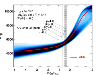
Figure 1: Left: Temperature stratification of the hydrodynamic model solar atmosphere used in this work; also shown is the temperature stratification of the temporally and horizontally averaged ⟨3D⟩ model solar atmosphere. Vertical lines are used to indicate the locations of the peaks of the temporally and horizontally averaged contribution functions at different inclinations. Right: Contribution functions to the absolute intensity depression for the individual components of the O I $777\,\mathrm{nm}$ triplet and at different inclinations, calculated on the full 3D model solar atmosphere and subsequently temporally and horizontally averaged. The contribution functions have been normalised individually, such that the area under each is equal to unity.

We illustrate the temperature stratification of the 3D hydrodynamic model solar atmosphere used in this work in Fig. 1. This is an updated version of the model used in Asplund et al. (2009) and Pereira et al. (2013), and was recently used in Lind et al. (2017) and Nordlander & Lind (2017). The model solar atmosphere was computed using a custom version of the stagger code (Nordlund & Galsgaard, 1995; Stein & Nordlund, 1998), tailored for the Sun. The code solves the discretised equations for the conservation of mass, momentum, and energy coupled with the radiative transfer equation for a representative volume of the solar surface on a Cartesian mesh.

The numerical grid for the simulation covers $240^{3}$ grid points, spanning $6$ Mm in each horizontal direction and $4$ Mm vertically. The simulation domain completely covers the Rosseland mean optical depth range ${-5}{\leq}\log_{10}\tau_{\mathrm{Ross}}{\leq}7$, spanning about $8$ and $6$ pressure scale heights above and below the optical surface ($\tau_{\mathrm{Ross}}$=0), respectively. Boundaries are open and transmitting at the top and bottom of the simulation, and periodic in the horizontal directions. At the bottom boundary, located in the upper part of the solar convection zone, the entropy of the inflowing gas and the gas pressure were set to constant values. A constant vertical gravitational acceleration with $\log_{10}\left(g/\mathrm{cm\,s^{-2}}\right)=4.44$ was enforced throughout the simulation domain.

The simulation used an updated version of the equation of state by Mihalas et al. (1988) and of the continuous opacity package by Gustafsson et al. (1975) (see Trampedach et al. 2013 and Hayek et al. 2010 for a comprehensive list of the included continuous opacity sources). Sampled line opacities for wavelengths between $90\,\mathrm{nm}$ and $20000\,\mathrm{nm}$ came from B. Plez (priv. comm.) and Gustafsson et al. (2008). The adopted chemical composition assumed for the calculation of the equation of state variables and opacities was taken from Asplund et al. (2009).

In order to compute the heating rates that enter the energy conservation equation, the radiative transfer in the layers with $\tau_{\mathrm{Ross}}{\leq}500$ were solved at each time step along rays crossing all grid points at the solar surface at nine inclinations (two $\mu$-angles and four $\phi$-angles, plus the vertical) using a Feautrier-like scheme (Feautrier, 1964). In the optically thick regions, the diffusion approximation was used instead.

The computational load for the solution of the radiative transfer was reduced by adopting the opacity binning (or multi-group opacity) method (Nordlund, 1982; Skartlien, 2000). Prior to the calculations, wavelengths were sorted into different bins based on their spectral ranges and on the strength of the associated opacity. Opacities in each bin were then appropriately averaged and the contributions from the monochromatic source functions were added together. During the simulation with the stagger code, the radiative transfer equation was solved for the average opacities and cumulative source functions in each opacity bins. Coherent, isotropic continuum scattering was included in the source function in the optically thick layers, and neglected in the optically thin layers. The heating rates were then computed at all grid points by integrating the solution to the radiative transfer equation over the solid angle and over all opacity bins. We refer the reader to Sect. 2.3 of Collet et al. (2011), and in particular to the second approach presented there, for further details on the radiative transfer scheme.

The effective temperature is not enforced; instead, we fine-tuned the value of the specific entropy per unit mass of the inflowing gas at the bottom boundary to obtain a resulting effective temperature value close to the observed one. The convective simulation was run for several convective turn-over timescales (about 21 hours of solar time) to ensure that thermal and dynamical relaxation were achieved: the mean effective temperature of the entire sequence is $5773\,\mathrm{K}$, with standard deviation $16\,\mathrm{K}$. This is very close to the reference solar value of $5772\,\mathrm{K}$ (Prša et al., 2016).

2.1.2 Averaged model

We also illustrate the temperature stratification of an averaged 3D model solar atmosphere (hereafter ⟨3D⟩) in Fig. 1. The sensitivity of the statistical equilibrium on different aspects of the non-LTE modelling was tested using this model solar atmosphere, instead of the full 3D model solar atmosphere, to save computational resources. The ⟨3D⟩ model was constructed by calculating the mean of two thermodynamic quantities in space (on surfaces of equal Rosseland mean optical depth) and in time: the logarithmic gas density, and the gas temperature to the fourth power. All other quantities were then computed consistently from these two quantities, the optical depth, and the equation of state.

2.1.3 Line-forming regions

It is interesting to briefly consider where the O I $777\,\mathrm{nm}$ triplet forms in the 3D model solar atmosphere. To that end, we illustrate in Fig. 1 contribution functions for the absolute intensity depression at different inclinations, integrated over wavelength: rCl CF&∝ ∫α_λ S^eff_λ  e^-τ_λ dλ ,
S^eff_λ= (α^l_λ/ α_λ)(I^c_λ- S^l_λ)  (Amarsi, 2015, integrand of Eq. 12). The function was computed at every grid-point of the seven snapshots (Sect. 2.2) of the model solar atmosphere, and subsequently temporally and horizontally averaged on surfaces of equal Rosseland mean optical depth, and area normalised. These plots were calculated using 3D non-LTE radiative transfer (Sect. 2.2), and using the model atom with inelastic collisions with neutral hydrogen based on the asymptotic two-electron model of Barklem (2017a) combined with the full, free electron model of Kaulakys (1985, 1986, 1991) with an oxygen abundance of $8.7\,\mathrm{dex}$ (Sect. 2.4.2).

The O I $777\,\mathrm{nm}$ triplet forms deep in the photosphere, as expected from their high excitation potentials. They form over an extended region; the contribution functions are skewed to higher optical depths by the deep line cores. For disk-centre profiles the peak in the contribution function is around $-0.4\lesssim\log{\tau_{\mathrm{Ross}}}\lesssim-0.1$, depending on the line component (the weaker components forming at greater optical depth), with full widths at half maxima of around $\Delta\log{\tau_{\mathrm{Ross}}}\approx 1.0$. For profiles observed closer to the limb the contribution functions shift to more optically thin regions, and also become broader. For example, at $\mu=0.2$ the peaks move to around $-0.9\lesssim\log{\tau_{\mathrm{Ross}}}\lesssim-0.6$, with full widths at half maximum of around $\Delta\log{\tau_{\mathrm{Ross}}}\approx 1.4$. This broadening reflects the inhomogeneous nature of the stable photosphere, with a larger contribution to the line formation occurring in localised regions of higher gas temperature.

2.1.4 Validation

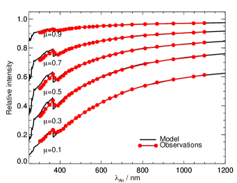
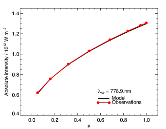
Figure 2: Left: Relative continuum intensities (normalised by the continuum intensity observed at disk-centre) at various inclinations as functions of wavelength, as predicted by the 3D hydrodynamic model solar atmosphere, and as given by the observations of Neckel & Labs (1994). Right: Absolute continuum intensity in the vicinity of the O I $777\,\mathrm{nm}$ triplet as a function of inclination, as predicted by the 3D hydrodynamic model solar atmosphere, and as given by the observations of Neckel & Labs (1994), put onto an absolute scale using the atlas of Neckel & Labs (1984).

Before using the centre-to-limb variation analysis to comment on the accuracy of the non-LTE modelling, it is necessary to first verify that the model solar atmosphere is an accurate representation of the quiet Sun.

In Fig. 2 we illustrate the centre-to-limb variation of the relative continuum intensity at different optical and near-infrared wavelengths, as predicted by the 3D hydrodynamic model solar atmosphere, and as given by the observations of Neckel & Labs (1994). We also compare the centre-to-limb variation of the absolute continuum intensity (emergent from the model solar atmosphere) in the vicinity of the O I $777\,\mathrm{nm}$ triplet, putting the data of Neckel & Labs (1994) onto an absolute scale using the disk-centre intensity atlas of Neckel & Labs (1984) and a small continuum window centred on $\lambda_{\text{Air}}=776.885\,\mathrm{nm}$.

Fig. 2 shows that redward of the Balmer discontinuity, the observed centre-to-limb variation is very well reproduced by the model, from disk-centre down to $\mu\approx 0.1$. This is strong evidence that the temperature stratification is realistic in the continuum-forming regions $-1.0\lesssim\log\tau_{\lambda}\lesssim 0.0$. Slight discrepancies at shorter wavelengths may indicate that some UV opacity is missing in our synthesis. In addition, Fig. 2 shows that the absolute continuum intensities are in good agreement, which mainly verifies that the effective temperature of the model solar atmosphere is correct.

For further validation, we note that the 3D hydrodynamic model solar atmosphere used here is the same one used by Lind et al. (2017) to analyse the centre-to-limb variations of ten Fe I lines and one Fe II line. They were generally able to reproduce the the centre-to-limb variations down to $\mu\approx 0.4$; disagreements closer to the limb can be explained by uncertainties in their non-LTE modelling. These eleven lines have different excitation potentials, oscillator strengths, and wavelengths; and consequently, different regions of line formation. We calculated the contribution functions for these lines in the same way as we did for the O I $777\,\mathrm{nm}$ triplet (Sect. 2.1.3), but under the assumption of LTE; this is valid because the non-LTE effects are small for Fe I lines in the Sun. For disk-centre profiles the peaks in the contribution function are in the range $-0.4\lesssim\log{\tau_{\mathrm{Ross}}}\lesssim-1.4$, while for profiles observed at $\mu=0.4$ the peaks are in the range $-0.9\lesssim\log{\tau_{\mathrm{Ross}}}\lesssim-1.6$. This covers and extends beyond the region in which the O I $777\,\mathrm{nm}$ triplet forms.

Finally, we comment on magnetic fields, which were neglected in our purely hydrodynamic simulations. The O I $777\,\mathrm{nm}$ triplet is sensitive to magnetic fields, both directly (via Zeeman broadening) and indirectly (via changes to the atmospheric structure), as shown by the MHD simulations of Fabbian et al. (2012), Fabbian & Moreno-Insertis (2015), Moore et al. (2015), and Shchukina et al. (2016). The first two studies imposed a vertical mean field of $100\,\mathrm{G}$ in their MHD simulations. This magnetic field topology has a large impact on the atmospheric structure, that promotes a strong indirect effect of magnetic fields on spectral line formation; as such, their results suggest abundance corrections can reach approximately $0.1\,\mathrm{dex}$, compared to the purely hydrodynamic case. In contrast, the last two studies adopted small-scale, self-dynamo models with mean strengths of $80$–$160\,\mathrm{G}$ in their MHD simulations. Their results suggest much smaller abundance corrections; for the O I $777\,\mathrm{nm}$ triplet these are only of the order of $0.01\,\mathrm{dex}$. Observations suggest that the small-scale dynamo approach is more realistic (e.g. Trujillo Bueno et al., 2004).

2.2 Line formation code

Our 3D non-LTE radiative transfer code balder, which is a custom version of multi3d (Botnen & Carlsson, 1999; Leenaarts & Carlsson, 2009), was used in this study. We refer the reader to Amarsi et al. (2018) and references therein for an overview of the code.

Calculations were performed across seven snapshots of the 3D hydrodynamic model solar atmosphere that we described in Sect. 2.1.1. These snapshots were equally spaced in solar time. Prior to performing line formation calculations, the snapshots were resampled onto a mesh with $80\times 80\times 220$ grid points, as described in Amarsi et al. (2018). Line formation calculations were performed for each model snapshot for different values of oxygen abundance $\log{\epsilon_{\mathrm{O}}}$, in steps of $0.2\,\mathrm{dex}$, under the assumption that these variations have no effect on the background atmosphere (i.e. that oxygen is a trace element).

The calculations on the ⟨3D⟩ model solar atmosphere proceeded in mostly the same way as those on the 3D hydrodynamic model solar atmospheres. In general, microturbulent and macroturbulent broadening (e.g. Gray, 2008, Chapter 17) need to be included in analyses based on 1D model atmospheres in order to reproduce the line broadening effects of the convective velocity field oscillations and temperature inhomogeneities (Asplund et al., 2000). In this work a depth-independent microturbulence of $\xi=1\,\mathrm{km\,s^{-1}}$ was adopted, and macroturbulence was included by convolving the profiles with Gaussian kernels of freely varying width $\varv_{\mathrm{mac}}\left(\mu\right)$ so as to best fit the observed profile.

2.3 Model atom

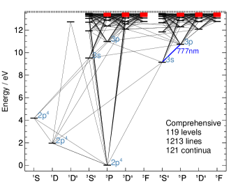
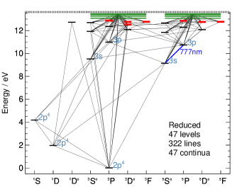
Figure 3: Grotrian diagram of O I in the comprehensive and reduced model oxygen atoms. Super levels are depicted as solid horizontal green lines. Levels that do not resolve fine structure are depicted as thick red lines; in the comprehensive atom, these correspond to levels taken from the Opacity Project. The final reduced model atom includes three levels of O II (fine structure collapsed), bringing the total number of levels to 50.

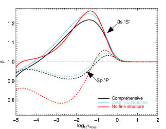
Figure 4: Departure coefficients for the lower and upper levels of the O I $777\,\mathrm{nm}$ triplet in the ⟨3D⟩ model solar atmosphere. The departure coefficients as predicted by the reduced model atom overlap with those predicted by the comprehensive model atom in this plot. Also shown are the departure coefficients predicted from the comprehensive model atom but with all fine structure above the triplet (i.e. above $10.74\,\mathrm{eV}$) collapsed (‘Less fine structure’), and from the comprehensive model atom but with all fine structure down to and including the ground level collapsed (‘No fine structure’), illustrating the importance of resolving fine structure in non-LTE model atoms.

We illustrate two model atoms in Fig. 3: a comprehensive model, which is more complete than those used in previous studies (e.g. Pereira et al., 2009a; Steffen et al., 2015; Amarsi et al., 2016), and a reduced model, which was used for the actual calculations at reduced computational cost but without significant loss of accuracy.

Experimental fine structure energies for O I up to $13.18\,\mathrm{eV}$ above the ground state (up to and including $\mathrm{6p\,^{3}P}$), and fine structure energies for O II up to $18.64\,\mathrm{eV}$ above the ground state (up to and including $\mathrm{2p^{3}\,{}^{2}P^{o}}$), were taken from the compilation of Moore (1993) via the NIST Atomic Spectra Database (Kramida et al., 2015). These were supplemented with all available O I energies given in the Opacity Project online database (TOPbase; Cunto et al., 1993).

Experimental O I oscillator strengths were taken from Hibbert et al. (1991) via the NIST Atomic Spectra Database. These were supplemented with all available O I oscillator strengths in TOPbase. The TOPbase data set does not include fine structure; we therefore carefully split the oscillator strengths under the assumption of pure LS coupling, using the tables given in Allen (1973, Sect. 27). Natural broadening coefficients were calculated using the lifetimes given in TOPbase, and van der Waals broadening coefficients, when possible, were based on the theory of Anstee, Barklem, and O’Mara (ABO; Anstee & O’Mara, 1995; Barklem & O’Mara, 1997; Barklem et al., 1998). Monochromatic photoionisation cross-sections were extracted from TOPbase.

The reduction broadly follows the procedure described in Amarsi & Asplund (2017, see Sect. 2.3.3 for details). First, eight O I super levels were constructed, starting at around $13.0\,\mathrm{eV}$ ($\mathrm{6s\,^{5}S^{o}}$). These super levels combine composite levels that share the same spin quantum number and are separated in energy by less than $0.1\,\mathrm{eV}$. They were were constructed by weighting the composite level energies according to their Boltzmann factors (adopting a characteristic temperature of $5000\,\mathrm{K}$). Affected lines and continua were collapsed into super lines and super continua.

Second, we considered collapsing the fine structure in the model atom. All fine structure in the O II system was collapsed; however, some care has to be taken with fine structure in O I (e.g. Steffen et al., 2015, Appendix B). Collapsing fine structure in O I can significantly impact the predicted departure coefficients; we illustrate this, using the ⟨3D⟩ model solar atmosphere, in Fig. 4. Although these differences ultimately only have a small impact on the O I $777\,\mathrm{nm}$ triplet in 1D model atmospheres (e.g. Kiselman, 1993), the impact may be larger on the line profiles emergent from 3D hydrodynamic model atmospheres. We therefore chose to be cautious, and resolved fine structure in O I levels up to around $12.5\,\mathrm{eV}$ (up to and including $\mathrm{4p\,^{3}P}$).

2.4 Inelastic collisions

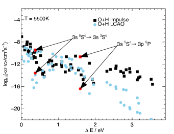
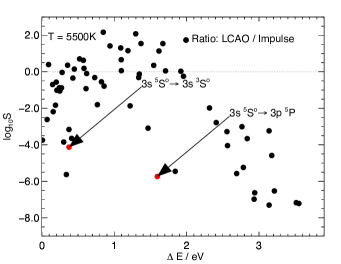
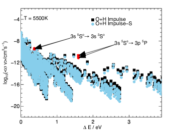
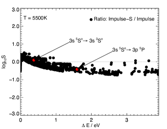
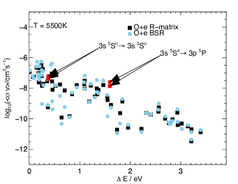
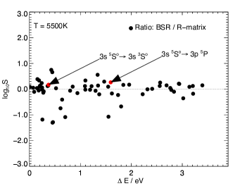
Figure 5: Excitation rate coefficients $\langle\sigma\varv\rangle$ for different models of inelastic collisions with neutral hydrogen atoms and with free electrons, and their ratios $S$, as functions of the transition energy and at a fixed temperature. LCAO refers to Barklem (2016b); Impulse refers to Kaulakys (1991, Eq. 9); Impulse-S refers to Kaulakys (1991, Eq. 18); R-matrix refers to Barklem (2007); BSR refers to Tayal & Zatsarinny (2016) (extended here to higher energies; see Sect. 2.4.3). The important $\mathrm{3s\,{{}^{5}}S^{o}}\rightarrow\mathrm{3s\,{{}^{3}}S^{o}}$ and $\mathrm{3s\,{{}^{5}}S^{o}}\rightarrow\mathrm{3p\,{{}^{5}}P}$ transitions have been highlighted.

2.4.1 Overview

The inelastic collisional processes in the model atom include oxygen plus neutral hydrogen (O+H) excitation, oxygen plus electron (O+e) excitation, oxygen plus proton (O+p) charge transfer (which is efficient for the transition between the ground states of O I and O II), O+e ionisation, and O+H charge transfer, from most to least influential on the O I $777\,\mathrm{nm}$ triplet strength. We discuss them in turn below.

Most of the collisional rate coefficient data discussed below were calculated without resolving fine structure. To include them into the model atom, which does include fine structure, we note that it is necessary to divide by the total number of final states so as to approximately preserve the total rate per perturber in dimensions of inverse time. This works because the collisional rates within fine structure in our models were set to very high values, so that the population ratios within fine structure levels are given by the ratios of their statistical weights (following Kiselman, 1993). This in turn can be justified since inelastic collision processes between fine structure levels are expected to be very efficient on the basis of the Massey criterion (Massey, 1949).

2.4.2 O+H excitation

Inelastic collisions with neutral hydrogen have by far the most influence on the emergent O I $777\,\mathrm{nm}$ triplet intensities, even at disk-centre (Sect. 4.2). Uncertainties in the adopted collisions therefore dominate the uncertainty in the synthetic spectra, and consequently in the inferred abundances. As we discussed in Sect. 1, contemporary studies typically use the Drawin recipe (Lambert, 1993, Appendix A, and references therein). Here, we do not discuss the Drawin recipe in any detail other than to point out that this model contains very little of the relevant quantum scattering physics (Barklem et al., 2011). We restrict ourselves to more physically motivated recipes in order to shed light on the true nature of inelastic O+H collisions in the solar photosphere.

• LCAO. This refers to the asymptotic two-electron model of Barklem (2016b), based on a linear combination of atomic orbitals (LCAO) approach for the molecular structure (i.e. potentials and radial couplings) of the O-H quasi-molecule, and the multichannel Landau–Zener model for the collision dynamics. It describes electron transfer at avoided ionic crossings through interaction of ionic and covalent configurations (see Barklem et al., 2011; Barklem, 2016a). The data were recently presented in Barklem (2017a), and preliminary data were employed in Pazira et al. (2017).

• Impulse. This refers to the free electron model of Kaulakys (1985, 1986, 1991) based on the impulse approximation. This model describes the momentum transfer between the perturbing hydrogen atom and the active electron (which is assumed to be free) on the target (oxygen) atom due to the scattering process between these two particles. The Barklem (2017b) code was used to evaluate Kaulakys (1991, Eq. 9), and more details can be found in Osorio et al. (2015). The rate coefficients were redistributed among spin states following Barklem (2016a, Eq. 8 and Eq. 9).

• Impulse-S. This also refers to the free electron model above (Impulse), but in the scattering length approximation (Kaulakys, 1991, Eq. 18). This approximation typically agrees with the full model to within a factor of three, while being approximately $3\,\mathrm{dex}$ cheaper to compute.

We show in Sect. 4.1 that the LCAO model alone is unable to reproduce the centre-to-limb variation of the O I $777\,\mathrm{nm}$ triplet. The reason for this can be understood by noting that the most important transitions for triplet formation in the photosphere are $\mathrm{3s\,{{}^{5}}S^{o}}\leftrightarrow\mathrm{3p\,{{}^{5}}P}$ and $\mathrm{3s\,{{}^{5}}S^{o}}\leftrightarrow\mathrm{3s\,{{}^{3}}S^{o}}$ (Sect. 4.2). As pointed out in Barklem (2017a), the relevant avoided crossings for these transitions occur at short range, and so the LCAO model gives rather low rates for these transitions. Consequently, the LCAO model by itself cannot reasonably be expected to give accurate rates for these transitions because there are likely to be contributions from mechanisms other than the radial couplings at avoided ionic crossings. In the standard adiabatic (Born–Oppenheimer) approach, these mechanisms correspond to rotational and spin-orbit coupling, and to additional radial couplings.

Compared to the LCAO model, the Impulse model employs a completely different approach to the structure and scattering problem and there is no obvious relationship between the two theories (e.g. Flannery, 1983). However, what is clear is that the avoided crossing mechanism is not included in the Impulse model: the model does not and cannot include ionic configurations because it assumes that the active electron on the target (oxygen) atomic nucleus is free. Thus, the Impulse and LCAO models do not have any overlap in the described physical mechanism.

Thus, in the absence of detailed full-quantum calculations in the standard adiabatic approach that include these other mechanisms, one possible approach is to add the rate coefficients from the LCAO model to those from the Impulse model (LCAO+Impulse) or, in order to reduce the computational cost of calculating the cross-sections, to those from the Impulse-S model (LCAO+Impulse-S). It should be noted that the Impulse approach contains a number of approximations which are generally valid only for Rydberg states (see Flannery, 1983). The application to $n=3$ states in oxygen is therefore questionable, but we use it to obtain an estimate of the possible contribution of other mechanisms in the absence of better alternatives.

We compare the relative magnitudes of the different models in Fig. 5. As expected, the Impulse model predicts much larger rate coefficients than the LCAO model for the important $\mathrm{3s\,{{}^{5}}S^{o}}\leftrightarrow\mathrm{3p\,{{}^{5}}P}$ and $\mathrm{3s\,{{}^{5}}S^{o}}\leftrightarrow\mathrm{3s\,{{}^{3}}S^{o}}$ transitions. Therefore, uncertainties propagating forward from the Kaulakys (1991) recipe dominate the overall uncertainties in the non-LTE modelling of the O I $777\,\mathrm{nm}$ triplet.

2.4.3 O+e excitation

After neutral hydrogen, inelastic collisions with free electrons have the most influence on the O I $777\,\mathrm{nm}$ triplet. Contemporary studies usually adopt the data presented in Barklem (2007), based on standard R-matrix calculations (e.g. Burke et al., 1971; Burke & Robb, 1976). For the first time, we adopt data based on B-spline R-matrix (BSR) calculations (Zatsarinny, 2006). The calculations for oxygen were presented in Tayal & Zatsarinny (2016), and extended for this work to include transitions up to around $12.65\,\mathrm{eV}$ above the ground state (up to and including $\mathrm{3s\,^{1}D^{o}}$).

We compare the two data sets in Fig. 5. The agreement is good with most transitions agreeing to better than a factor of two. For the important $\mathrm{3s\,{{}^{5}}S^{o}}\leftrightarrow\mathrm{3p\,{{}^{5}}P}$ transition, the new data are a factor of two larger at the relevant temperatures. However, given the overwhelming importance of the O+H excitation collisions (Sect. 4.2), adopting the newer data set only affects the inferred abundances by less than $0.01\,\mathrm{dex}$, with our adopted model atom and LCAO+Impulse description for inelastic O+H collisions (Sect. 2.4.2).

2.4.4 O+p charge transfer

The O+p charge transfer rate coefficients for the transition coupling the ground states of O I and O II were taken from Stancil et al. (1999), based on a combination of various quantal and semi-classical theoretical calculations and on experimental data. As pointed out by e.g. Steffen et al. (2015), this transition ensures that the two levels share the same departure coefficients. Since the ground state of O I is guaranteed to be in LTE (by virtue of the high ionisation potential of O I) the effect of this transition is thus to ensure the O II level is also in LTE.

2.4.5 O+e ionisation

O+e ionisation rate coefficients were calculated using the empirical formula from Allen (1973). Our tests suggest that the formula is accurate to around a factor of two. In any case, these rates do not play a major role in the statistical equilibrium of O I, as we discuss in Sect. 4.2.

2.4.6 O+H charge transfer

O+H charge transfer rate coefficients were drawn from the same calculations as the LCAO model we described in Sect. 2.4.2: the data were presented in Barklem+, based on the asymptotic two-electron model presented in Barklem (2016b). Pazira et al. (2017) discussed the importance of these transitions on the faint O I $777\,\mathrm{nm}$ triplet emission in the lower chromosphere. In the photosphere, however, these transitions are apparently much less important (Sect. 4.2).

3 Analysis

3.1 Observations

The quiet-Sun observations of Pereira et al. (2009b), averaged in space and time and normalised by (Pereira et al., 2009a), were used to analyse the centre-to-limb variation of the O I $777\,\mathrm{nm}$ triplet. These data were also used in the study of Steffen et al. (2015), as we discussed in Sect. 1. They were acquired using the TRI-Port Polarimetric Echelle-Littrow (TRIPPEL) spectrograph (Kiselman et al., 2011) on the Swedish 1-m Solar Telescope (SST; Scharmer et al., 2003) in May 2007.

The observations were of five $\mu=\cos\theta$ locations across the solar disk: $\mu=0.197\pm 0.003$, $0.424\pm 0.024$, $0.608\pm 0.020$, $0.793\pm 0.012$, and $0.999\pm 0.001$; the uncertainty in $\mu$ originates from the finite spatial coverage of the slit. The instrumental profile is approximately Gaussian with full width at half maximum $\varv_{\mathrm{b}}\approx 1.50\,\mathrm{km\,s^{-1}}$ (Pereira et al., 2009b).

3.2 Fitting procedure

The following analysis is based on directly fitting the observed spectra, instead of an approach based on measured equivalent widths. The model spectra were convolved with the instrumental profile before comparing them to the observed spectra. All three components of the O I $777\,\mathrm{nm}$ triplet for a given $\mu$-pointing were fit simultaneously.

There are some weak blending lines, mainly of CN and C₂, in the region around the O I $777\,\mathrm{nm}$ triplet. Pereira et al. (2009a, Sect. 4.1.4) reported that these blends have a small influence on their calibration of $S_{\mathrm{H}}$, and, more relevant to this work, a negligible affect on the oxygen abundances inferred by profile fitting. Consequently, we neglect these blends from our analysis, which is also the approach taken by both Pereira et al. (2009a) and Steffen et al. (2015).

The profiles were fit by unweighted $\chi^{2}$ minimisation, using the IDL routine MPFIT (Markwardt, 2009). For the 3D non-LTE analyses and a given $\mu$-pointing, the main free parameter is the oxygen abundance. The other free parameter (for a given $\mu$-pointing) is a global wavelength shift (affecting all three components of the O I $777\,\mathrm{nm}$ triplet in the same way). This was necessary to account for uncertainties in the absolute wavelength calibration (Pereira et al., 2009a).

For the 3D non-LTE analyses, no extra broadening parameters (microturbulence $\xi$; macroturbulence $\varv_{\mathrm{mac}}$) were included. The broadening effects of the convective velocity field oscillations and temperature inhomogeneities are implicit in the 3D non-LTE method (Asplund et al., 2000). However, as we discussed in Sect. 2.1.2, the analyses based on the ⟨3D⟩ model solar atmosphere also included macroturbulence as a free parameter, $\varv_{\mathrm{mac}}\left(\mu\right)$.

3.3 Fits

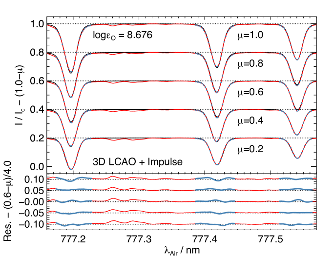
Figure 6: Observed (red line) and theoretical (black line) centre-to-limb variation of the O I $777\,\mathrm{nm}$ triplet using the 3D hydrodynamic model solar atmosphere and our best description for the inelastic O+H collisions (Sect. 2.4.2). The oxygen abundance was fit for $\mu=1.0$, and fixed to this value for the other $\mu$-pointings. In the top panel the observational data used in the fit (blue dots) have been subsampled by a factor of two to make it easier to see the theoretical spectra below it. In the bottom panel, the residual is defined as the theoretical minus the observed spectra.

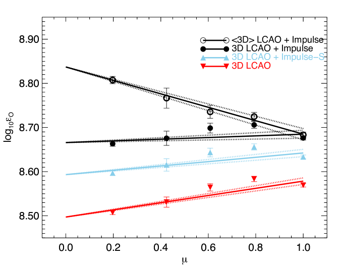
Figure 7: Abundances inferred by fitting the observed spectra at the different $\mu$-pointings individually using the 3D hydrodynamic model solar atmosphere and different descriptions for the inelastic O+H collisions (Sect. 2.4.2); our best description is the LCAO+Impulse model, based on physical arguments. The same abundance should be inferred from each $\mu$-pointing (i.e. a flat line is expected). The error bars were calculated by combining in quadrature the uncertainties arising from the finite slit-width (or spread in $\mu$), a $0.1\%$ uncertainty in the continuum placement, and the formal fitting error; the first error dominates for the three intermediate pointings, while the last two errors are important for $\mu\approx 0.2$ and $\mu\approx 1.0$. Solid lines of weighted best fit are overdrawn, and the dashed lines illustrate the $1\,\sigma$ uncertainty in the fitted gradients.

In Fig. 6, we illustrate how the observed spectra compare to the 3D non-LTE model spectra with the LCAO+Impulse description for the inelastic O+H collisions that we described in Sect. 2.4.2. The oxygen abundance was fit to the disk-centre spectra, then fixed to this value for the other $\mu$-pointings.

In Fig. 7, we show the inferred oxygen abundances after fitting the different $\mu$-pointings separately, as a function of $\mu$, using the ⟨3D⟩ model solar atmosphere with the main, LCAO+Impulse description for the inelastic O+H collisions, and the full 3D model solar atmosphere with different descriptions for the inelastic O+H collisions.

4 Discussion

4.1 Models versus observations

Fig. 6 illustrates that the 3D non-LTE, LCAO+Impulse model reproduces the strengths and shapes of the lines reasonably well across the solar disk. It is apparent, however, that the synthetic lines are not broad enough. We speculate that this can be explained by Zeeman broadening, which is neglected in our purely hydrodynamic simulations. This imparts a systematic error on our fitted abundances; however, this error is expected to be small (of the order of $0.01\,\mathrm{dex}$; e.g. Moore et al., 2015; Shchukina et al., 2016).

Fig. 7 demonstrates that when using the 3D non-LTE, LCAO+Impulse model for the inelastic collisions (Sect. 2.4.2), the inferred oxygen abundances are consistent across the solar disk to a scatter of $\pm 0.02\,\mathrm{dex}$. The weighted mean abundance is the same as the unweighted mean abundance, namely $8.684\,\mathrm{dex}$. The scatter is larger than the mean trend (the line of best fit), which gives $8.685\,\mathrm{dex}$ at disk-centre and $8.666\,\mathrm{dex}$ when extrapolated to $\mu=0.0$, a discrepancy of just $0.02\,\mathrm{dex}$.

The centre-to-limb discrepancy of $0.02\,\mathrm{dex}$ using the 3D model solar atmosphere in Fig. 7 could signal that the the LCAO+Impulse model may slightly underestimate the inelastic O+H collisions overall. However, we caution that this analysis cannot be used to comment on the relative errors between different transitions. This is why a physically motivated approach is beneficial. We would hope, if the same physics describes all of these transitions, that the relative error between transitions is negligible. The scatter of $\pm 0.02\,\mathrm{dex}$ about the mean trend of centre-to-limb abundances is inconsistent with the $1\,\sigma$ observational uncertainties. We stress that the scatter is unlikely to be associated with the treatment of inelastic O+H collisions, and that the scatter does not alter our conclusions about the inelastic O+H collisions. We note, however, that residual systematic errors such as these interfere with attempts to calibrate the inelastic O+H collisions and $S_{\mathrm{H}}$.

We also cannot completely rule out errors in other aspects of the modelling and analysis, as the cause of the residual mean trend and scatter of the order of $0.02\,\mathrm{dex}$. For example, the pronounced difference between the ⟨3D⟩ and full 3D trends indicate a sensitivity to the model solar atmosphere; however, the evidence suggests that the hydrodynamics of the solar photosphere can be modelled with sufficient accuracy, at least in the regions where the O I $777\,\mathrm{nm}$ triplet forms, as we discussed in Sect. 2.1.4. As we mentioned above, Zeeman broadening is neglected in the models, and differences of about $0.02\,\mathrm{dex}$ may be present. Finally, these small discrepancies could reflect a systematic error in the observed spectra, for example in the treatment of stray light or in the accuracy of the value of $\mu$ (Pereira et al., 2009b).

We briefly consider the alternative descriptions for the inelastic O+H collisions. Using the LCAO+Impulse-S model (Sect. 2.4.2), the weighted mean abundance drops to $8.627\,\mathrm{dex}$; Fig. 7 displays a more prominent trend of decreasing inferred abundance moving from disk-centre to the limb. The model spectra are too strong at the limb, relative to disk-centre. Compared to the LCAO+Impulse model above, this difference can largely be attributed to the rate coefficients for the important $\mathrm{3s\,{{}^{5}}S^{o}}\rightarrow\mathrm{3p\,{{}^{5}}P}$ transition (Sect. 4.2) being a factor of $2.65$ smaller in the Impulse-S model compared to in the Impulse model (Fig. 5).

In Fig. 7 we also show results calculated using the LCAO model alone. The weighted mean abundance drops to $8.547\,\mathrm{dex}$, which is anomalously low (compared to the abundances inferred from other diagnostics; e.g. Asplund et al., 2009) and Fig. 7 displays a very prominent trend of decreasing inferred abundance moving from disk-centre to the limb. The model spectra are again too strong at the limb, relative to disk-centre. As we discussed in Sect. 2.4.2, this suggests that the mechanism described by the LCAO model, namely electron transfer at avoided ionic crossings, is not the dominant mechanism for the important $\mathrm{3s\,{{}^{3}}S^{o}}\rightarrow\mathrm{3s\,{{}^{5}}S^{o}}$ and $\mathrm{3p\,{{}^{5}}P}\rightarrow\mathrm{3s\,{{}^{5}}S^{o}}$ transitions (Sect. 4.2), which occur at short range.

Finally, we briefly comment on the LTE assumption. For clarity, we do not show the 3D LTE results in Fig. 7. The inferred abundance at disk-centre in 3D LTE is $8.88\,\mathrm{dex}$, and this steeply increases towards the limb by around $0.6\,\mathrm{dex}$. The centre-to-limb variation clearly rules out LTE as a valid modelling assumption (e.g. Altrock, 1968).

4.2 Sensitivity to the inelastic O+H collisions

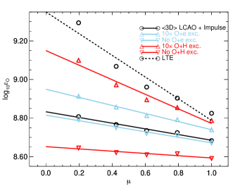
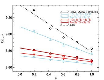
Figure 8: Abundances inferred at the different $\mu$-pointings using the ⟨3D⟩ model solar atmosphere. The same abundance should be inferred from each $\mu$-pointing (i.e. a flat line is expected). The left plot shows the effect of altering all inelastic O+e or O+H excitation rate coefficients. The right plot shows the effect of altering the inelastic O+e and O+H excitation rate coefficients (simultaneously) for the specified transition.

As we explained in Sect. 2.1.2, we used the ⟨3D⟩ model solar atmosphere to test the sensitivity of the centre-to-limb variation of the O I $777\,\mathrm{nm}$ triplet to different aspects of the non-LTE modelling. We illustrate the sensitivity to different inelastic collisional transitions in Fig. 8. The inelastic O+H excitation collisions have the largest influence on the statistical equilibrium. Switching them off reduces the abundance inferred from the disk-centre spectra by $0.09\,\mathrm{dex}$, while enhancing them by a factor of ten increases the abundance inferred from the disk-centre spectra by $0.10\,\mathrm{dex}$.

The inelastic O+e collisions have a smaller but still significant influence on the statistical equilibrium. Although switching them off reduces the abundance inferred from the disk-centre spectra by only $0.01\,\mathrm{dex}$, enhancing them by a factor of ten increases the abundance inferred from the disk-centre spectra by $0.06\,\mathrm{dex}$.

The other types of inelastic collisional transitions included in the model, O+p charge transfer, O+e ionisation collisions, and O+H charge transfer, have a much smaller impact on the O I $777\,\mathrm{nm}$ triplet. For clarity, we do not show them in Fig. 8. Switching them off or enhancing them by a factor of $10$ affects the abundances inferred from the disk-centre spectra by much less than $0.01\,\mathrm{dex}$.

The most important inelastic collisional transition for the O I $777\,\mathrm{nm}$ triplet is the radiatively allowed transition between $\mathrm{3s\,{{}^{5}}S^{o}}$ and $\mathrm{3p\,{{}^{5}}P}$ (i.e. between the levels of the triplet). The transition directly offsets the photon losses in the triplet (Amarsi et al., 2016). Fig. 8 shows that switching it off reduces the abundance inferred from the disk-centre spectra by $0.05\,\mathrm{dex}$, while enhancing it by a factor of ten increases the abundance inferred from the disk-centre spectra by $0.08\,\mathrm{dex}$.

The second most important inelastic collisional transition is the radiatively forbidden, spin-exchange transition between $\mathrm{3s\,{{}^{5}}S^{o}}$ (i.e. the lower level of the O I $777\,\mathrm{nm}$ triplet) and $\mathrm{3s\,{{}^{3}}S^{o}}$. It efficiently reduces the overpopulation of the metastable $\mathrm{3s\,{{}^{5}}S^{o}}$ level (e.g. Pazira et al., 2017). Fig. 8 shows that switching it off reduces the abundance inferred from the disk-centre spectra by $0.02\,\mathrm{dex}$. Enhancing it by a factor of ten has a negligible impact on the triplet strength; in the present model, the collisions are already efficient enough to ensure that these two levels share the same departure coefficients.

4.3 Solar oxygen abundance

We comment on the implications of our results on the still disputed solar oxygen abundance. To infer the solar oxygen abundance from the O I $777\,\mathrm{nm}$ triplet, it makes sense to use the disk-centre spectra, since here the observed lines have formed deeper in the atmosphere. This means that the abundance inferred from the disk-centre spectra is less influenced by the inelastic O+H collisions and by departures from LTE, which would otherwise dominate the overall uncertainty. Also, the disk-centre spectra and its normalisation has already been shown (Pereira et al., 2009a) to compare well with the high-resolution disk-centre solar atlas of Neckel & Labs (1984); it is thus unlikely that there are severe systematic errors in the disk-centre observational data set.

The 3D non-LTE, LCAO+Impulse model gives a disk-centre abundance of $8.676\,\mathrm{dex}$ from the O I $777\,\mathrm{nm}$ triplet (Fig. 6). However, as we discussed in Sect. 4.1, this model gives a slight gradient in the mean trend of inferred abundances of about $+0.02\,\mathrm{dex}$ going from the limb to disk-centre. We make the assumption that the inelastic O+H rate coefficients are the dominant source of error; a reasonable assumption for the Impulse model. The $\mathrm{3s\,{{}^{5}}S^{o}}\rightarrow\mathrm{3p\,{{}^{5}}P}$ transition dominates in importance (Sect. 4.2). Separate calculations showed that enhancing the rate coefficient of the $\mathrm{3s\,{{}^{5}}S^{o}}\rightarrow\mathrm{3p\,{{}^{5}}P}$ transition by a factor of two leads to a disk-centre abundance of $8.709\,\mathrm{dex}$, and the opposite gradient in the mean trend of centre-to-limb abundances ($-0.02\,\mathrm{dex}$).

Thus, by flattening the residual trend in the 3D non-LTE, LCAO+Impulse model in this way, we obtain a recommended solar oxygen abundance: $\log{\epsilon_{\mathrm{O}}}=8.69\pm 0.03$. The uncertainty of $0.03\,\mathrm{dex}$ combines the scatter about the mean trend of centre-to-limb abundances from the 3D non-LTE, LCAO+Impulse model ($\pm 0.02\,\mathrm{dex}$), the uncertainty in this rough calibration of the $\mathrm{3s\,{{}^{5}}S^{o}}\rightarrow\mathrm{3p\,{{}^{5}}P}$ transition ($\pm 0.02\,\mathrm{dex}$, half the difference between the two disk-centre inferred abundances), errors in the oscillator O I $777\,\mathrm{nm}$ triplet (of the order $\pm 0.01\,\mathrm{dex}$; Kramida et al., 2015), and the errors incurred from neglecting magnetic fields (also of the order $\pm 0.01\,\mathrm{dex}$: e.g. Moore et al., 2015; Shchukina et al., 2016).

This result agrees with the low solar oxygen abundance of $\log{\epsilon_{\mathrm{O}}}=8.69\pm 0.05$ advocated by Asplund et al. (2009). Such a low solar oxygen abundance is still controversial because it increases the disagreement between predictions from standard solar interior models and helioseismic measurements for the depth of the convection zone, the helium abundance in the convective envelope, and the interior sound speed in the Sun (e.g. Serenelli, 2016; Turck-Chièze, 2016).

The cause for this solar modelling problem has been extensively investigated since the first 3D-based studies implying a low ($\log{\epsilon_{\mathrm{O}}}\approx 8.70$) solar abundance appeared (Allende Prieto et al., 2001; Asplund et al., 2004), but as yet without a conclusive resolution. Recent findings of substantial amount of missing opacity in the solar interior, however, suggest that this long-standing problem may soon be solved. Bailey et al. (2015) measured iron opacities in conditions close to those near the base of the convection zone with the Sandia $Z$-pinch machine. Their measured Rosseland mean opacities for iron were a factor of around $1.75$ higher than predicted (by standard opacity models; e.g. Iglesias & Rogers, 1996; Iglesias et al., 2003; Badnell et al., 2005). This implies that iron alone can explain about half of the solar modelling problem. Complementing this, new R-matrix calculations found that the Rosseland mean opacity for the important Fe XVII ion is enhanced by a factor of around $1.35$ after including atomic core photoexcitations as well as other improvements (Nahar & Pradhan, 2016a, b; Pradhan & Nahar, 2018); ensuring completeness of excited configurations leads to an additional enhancement of around $1.20$ (Zhao et al., 2018). These results suggest that a resolution may be reached without having to revise the abundance of oxygen (or other key elements) in the solar atmosphere.

4.4 Proposed recipe for inelastic X+H collisions

In Sect. 2.4.2, we briefly motivated the LCAO+Impulse model from a theoretical perspective, and in Sect. 4.1 we demonstrated that this model can reproduce the solar centre-to-limb variation of the O I $777\,\mathrm{nm}$ triplet, albeit with some evidence of a discrepancy (of about $0.02\,\mathrm{dex}$), which may indicate that the inelastic O+H collisions are slightly underestimated overall.

There is evidence of the validity of the LCAO and Impulse models from other studies that have applied them separately. In particular, Barklem (2016b) showed that the LCAO model cross-sections for Li I, Na I, and Mg I compared well with those of detailed full-quantum calculations for transitions with high rates. The detailed full-quantum calculations in turn agree with experiment for the one available case, Na I $3s\rightarrow 3p$ (Fleck et al., 1991; Belyaev et al., 1999; Barklem et al., 2011). It has previously been demonstrated that the latter data sets, when incorporated into non-LTE model atoms, are needed to accurately model low- and intermediate-excitation lines (Lind et al., 2009, 2011; Osorio et al., 2015).

In contrast, transitions between levels of high excitation are typically in the regime of the Impulse model. Osorio et al. (2015) presented non-LTE Mg I calculations based on 1D and ⟨3D⟩ model atmospheres, and was able to reproduce the solar centre-to-limb variation of high-excitation Mg I emission lines after adopting the Impulse model for the inelastic Mg+H collisions.

In the absence of detailed full-quantum scattering calculations based on quantum chemistry calculations of the molecular structure, it is desirable to have some physically motivated, approximate description for inelastic X+H collisions to use in non-LTE model atoms. The results presented here, and in the studies discussed above, signal that the LCAO+Impulse may work to a satisfactory level of accuracy. We caution, however, that this needs to be tested against, for example, the centre-to-limb variation of other species using 3D non-LTE line formation calculations. In particular, the Impulse model employs a number of approximations that increase the uncertainty of the calculated rate coefficients (e.g. Barklem, 2016a), and it may just be coincidental that the model performs well for the handful of inelastic O+H transitions that are most important (Sect. 4.2) for the line formation of the O I $777\,\mathrm{nm}$ triplet.

The computational cost of the Impulse model (Kaulakys, 1991, Eq. 9) can make it impractical for modelling more complex chemical species such as Fe I/Fe II. In that case a cheaper alternative may be found in the Impulse-S model (Kaulakys, 1991, Eq. 18). The results in Fig. 7 show that the error is of the order of $0.06\,\mathrm{dex}$ (in terms of oxygen abundance) for the O I $777\,\mathrm{nm}$ triplet. However, other lines and species are typically less sensitive to the inelastic neutral hydrogen collisions, so this error of the Impulse-S model relative to the full Impulse model might be considered an upper bound. The difference between the Impulse-S model and the Impulse model may in general be less than the overall uncertainty in the Impulse model.

5 Conclusion

We have presented 3D non-LTE line formation calculations for the O I $777\,\mathrm{nm}$ triplet on a 3D hydrodynamic stagger model solar atmosphere. For the inelastic O+H collisions, we used the asymptotic two electron model, based on linear combinations of atomic orbitals, and the free electron model, based on the impulse approximation. This is more physically motivated than the often-used Drawin recipe, and may therefore lead to more trustworthy non-LTE model spectra and abundances.

The 3D non-LTE, LCAO+Impulse model compares well against the observed solar centre-to-limb variation of the O I $777\,\mathrm{nm}$ triplet. The mean trend of centre-to-limb abundances is almost flat, with a gradient of about $+0.02\,\mathrm{dex}$ going from the limb to disk-centre. This was achieved without any calibration of the inelastic collisional rate coefficients, and without ad hoc line broadening parameters. Given the success of the LCAO+Impulse model, and in the absence of detailed quantum chemistry calculations, we tentatively suggest adopting this approach for inelastic collisions in non-LTE models of other chemical species. We caution, however, that this hypothesis needs to be tested first, for example by performing analogous centre-to-limb variation analyses on other chemical species sensitive to inelastic collisions with neutral hydrogen.

After flattening the residual trend in the 3D non-LTE, LCAO+Impulse model, our recommended solar oxygen abundance from the O I $777\,\mathrm{nm}$ triplet is $\log{\epsilon_{\mathrm{O}}}=8.69\pm 0.03$, the error being dominated by systematics. This strengthens the case for a low solar oxygen abundance.

By combining 3D non-LTE modelling with advances in atomic physics, we can attempt to model O I spectral line formation in cool stars from first principles. In the absence of freely varying fudge parameters ($\xi$, $\varv_{\text{mac}}$, mixing length parameters, van der Waals damping enhancements, $S_{\mathrm{H}}$), deficiencies inherent in the models become apparent. In this work, for example, the LCAO model alone failed to predict the centre-to-limb variation of the O I $777\,\mathrm{nm}$ triplet, and that led us to develop the improved model presented in this work. Future work should apply the 3D non-LTE method to other spectral lines and chemical species to better understand line-formation from first principles and to provide fresh insight into the physics of planets, stars, and our Galaxy. As stated by Barklem (2017a), modern quantum chemistry calculations including potentials and couplings and detailed scattering calculations for the low-lying excited states of OH would be very important in this context.