Discovery and characterisation of long-period eclipsing binary stars from Kepler K2 campaigns 1, 2 and 3,

Abstract

Context. The Kepler K2 mission now makes it possible to find and study a wider variety of eclipsing binary stars than has been possible to-date, particularly long-period systems with narrow eclipses.

Aims. Our aim is to characterise eclipsing binary stars observed by the Kepler K2 mission with orbital periods longer than $P\approx 5.5$ days.

Methods. The ellc binary star model has been used to determine the geometry of eclipsing binary systems in Kepler K2 campaigns 1, 2 and 3. The nature of the stars in each binary is estimated by comparison to stellar evolution tracks in the effective temperature – mean stellar density plane.

Results. 43 eclipsing binary systems have been identified and 40 of these are characterised in some detail. The majority of these systems are found to be late-type dwarf and sub-giant stars with masses in the range 0.6 – 1.4 solar masses. We identify two eclipsing binaries containing red giant stars, including one bright system with total eclipses that is ideal for detailed follow-up observations. The bright B3V-type star HD 142883 is found to be an eclipsing binary in a triple star system. We observe a series of frequencies at large multiples of the orbital frequency in BW Aqr that we tentatively identify as tidally induced pulsations in this well-studied eccentric binary system. We find that the faint eclipsing binary EPIC 201160323 shows rapid apsidal motion. Rotational modulation signals are observed in 13 eclipsing systems, the majority of which are found to rotate non-synchronously with their orbits.

Conclusions. The K2 mission is a rich source of data that can be used to find long period eclipsing binary stars. These data combined with follow-up observations can be used to precisely measure the masses and radii of stars for which such fundamental data are currently lacking, e.g., sub-giant stars and slowly-rotating low-mass stars.

1 Introduction

Apart from the Sun and a few nearby stars, detached (i.e., non-interacting) eclipsing binaries (DEBS) provide the only means to measure accurate, model-independent masses and radii for normal stars. Using high-quality multi-wavelength photometry and high-resolution spectroscopy, masses and radii for stars in DEBS can be measured to $\pm 0.5$% or better (e.g., Maxted et al. 2015; Graczyk et al. 2016). Spectral disentangling techniques also make it possible to determine the effective temperature (T_eff) and surface composition of both stars in the binary from the analysis of their spectra (Pavlovski & Hensberge 2010). As a result, DEBS provide the most stringent test available for the accuracy of stellar evolution models for many different types of star (Torres et al. 2010). Empirical relations between mass, density, T_eff and metallicity based on DEBS can be used to estimate model-independent masses and radii for low-mass companions in SB1 eclipsing binaries, e.g., transiting hot-Jupiter systems (Southworth 2011) or brown dwarf or very low mass stars in eclipsing binaries with solar-type stars (Triaud et al. 2013). DEBS are also useful as distance indicators because their absolute magnitudes can be accurately estimated from the radii of the stars combined with a calibration of the stars’ surface brightness against colour or T_eff (Graczyk et al. 2017). DEBS have been used to investigate the systematic errors in parallax measurements for the Gaia DR1 data release (Stassun & Torres 2016a), and to accurately measure the distance to the Magellanic Clouds (Pietrzyński et al. 2013; Graczyk et al. 2014).

The Kepler K2 mission is providing very high quality photometry for thousands of moderately bright stars in selected regions of the sky (“campaign fields”) near the ecliptic plane (Howell et al. 2014). Each campaign field is observed almost continuously for up to 80 days, making it possible to discover and characterise eclipsing binaries with orbital periods of weeks that are very hard to study using light curves obtained from ground-based instruments. Extracting high quality photometry from the K2 images is challenging because the spacecraft is being operated using only 2 reaction wheels. This operating mode has made it possible to extend the mission lifetime, but does result in the pointing of the spacecraft being less stable than during the original Kepler mission. Nevertheless, there is now a variety of algorithms available to correct for the instrumental noise caused by this pointing drift that make it possible to recover photometric performance better than 100 ppm per 6-hours at 12th magnitude, close to the performance of the original Kepler mission (Luger et al. 2016; Aigrain et al. 2016; Vanderburg & Johnson 2014; Armstrong et al. 2015; Barros et al. 2016). These algorithms are generally optimised for the detection of the periodic shallow eclipses in the light curves of transiting exoplanets. Eclipsing binary stars have been found both as a by-product of these searches for transiting exoplanets and by searches for variable stars of all types in the Kepler K2 data. To-date, the characterisation of these eclipsing binaries has not been very detailed, being limited to estimates of the period plus, in some cases, some basic characterisation of the eclipse properties, e.g., depth and width.

At the time of writing, there are approximately 200 DEBS that have masses and radii measured to a precision of 2% or better (Southworth 2015). This sample is dominated by short-period systems ($P\loa 10$ d) in which the components of the binary system are forced to co-rotate with the orbit. This makes it difficult to study phenomena such as interior mixing processes that can have subtle effects on the evolution of normal stars, but which may be disrupted by rapid rotation, particularly for sub-giant and giant stars.

We have conducted our own search of the Kepler K2 data from campaigns 1, 2 and 3 and characterised the stars in these binaries in some detail using modelling of the Kepler K2 light curve plus existing optical and infrared photometry. Our study is motivated by the opportunity to study in detail stars of a type for which little fundamental accurate data are currently available. We have concentrated on bright stars with well-defined eclipses and long orbital periods that are ideal for detailed characterisation using high-resolution spectroscopy, but also discuss some other DEBS of interest that we have found in our survey. The results are presented here for the benefit of those who can share the task of characterising these binary systems and as a useful indicator of the number and properties of long-period eclipsing binaries that will be found in future large-scale photometric surveys.

2 Analysis

Note that where we refer to the primary and secondary stars in the following description (star 1 and 2, respectively) these labels refer to the star eclipsed during the deeper and shallower eclipses in the K2 light curve, respectively, irrespective of the stars’ effective temperatures, masses, radii, etc.

2.1 Target selection

Targets were identified by visual inspection of the detrended light curves generated by the k2sff algorithm (Vanderburg & Johnson 2014). We downloaded the light curve data from the Mikulski Archive for Space Telescopes (MAST) and used a simple script to plot the data for each system while making a note of any stars showing eclipse-like features in the light curve at least 5% deep and with orbital periods $P\ga 5.5$ days. We excluded stars from our list with a strong ellipsoidal effect in the light curve, i.e., a quasi-sinusoidal variation in flux with two maxima per orbital cycle due to the gravitational distortion of the stars in a close binary system. We also excluded systems fainter than Kepler magnitude ${\rm Kp}\approx 13$ unless they seemed particularly interesting based on an initial appraisal of the light curve or other information available. These points of interest are noted in section 3.1.

The list of stars selected for further analysis is shown in Table 1 together with some basic characteristics of the light curves. The rotation periods $P_{\rm rot}$ listed in this table were determined as part of the detrending process described in section 2.2.

2.2 Aperture photometry and detrending

We downloaded the target pixel files for each target from MAST and used these data to produce light curves using synthetic aperture photometry. We first calculated the median value for every pixel in the data cube. The pixels in the lowest 10-percentile of this median image were then used to calculate the background level in the individual images. We used the target aperture specified in the target pixel file where available, otherwise we used a circular aperture centered on the flux-weighted centroid of the median image with a radius selected by-eye to encompass most of the flux in the star – typically 4 – 8 pixels. We also calculated the flux-weighted centroid within the target aperture for each image.

The light curves produced by this method clearly show instrumental noise due to the varying position of the star on the detector. We used the k2sc algorithm (Aigrain et al. 2016) to remove this instrumental noise. This algorithm uses Gaussian processes to decompose the light curve into a trend associated with the position of the star on the detector plus a trend with time that represents the intrinsic variability of the star. We first detrend the data using a squared-exponential kernel to describe the covariance properties of the trend with time. This kernel is suitable for smooth, aperiodic variations so we mask the eclipses for this calculation. We then use a Lomb-Scargle periodogram (Press et al. 1992) to characterise any periodic or quasi-periodic variability in the detrended light curve between the eclipses. This variability can be due to modulation of the light curve by star spots on one or both stars, or due to pulsations. The periods that we judged to be significant detected by this process are noted in Table 1 and are listed in order of power from strongest to weakest. For the stars whose period is noted in Table 1 we repeated the detrending using a quasi-periodic kernel for the time trend, again with the eclipses masked. In both cases (squared-exponential and quasi-periodic kernels) the trend with position determined from the data between the eclipses was used to interpolate a correction to the data during the eclipses. f These light curves are shown in Figs. 1, 2, 3 and 4.

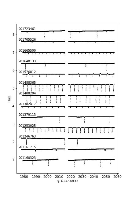
Figure 1: Light curves of long-period eclipsing binaries from Kepler campaign 1. The flux is measured relative to the median out-of-eclipse level and offset by multiple of 0.5 units for clarity. Trends in the data due to variations in spacecraft pointing have been removed.

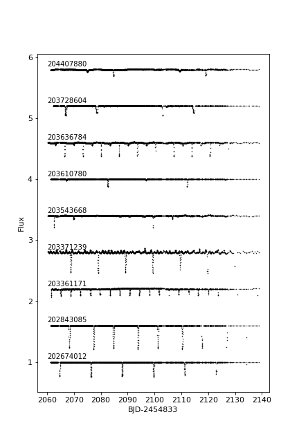
Figure 2: Light curves of long-period eclipsing binaries from Kepler campaign 2. The flux is measured relative to the median out-of-eclipse level and offset by multiple of 0.5 units for clarity. Trends in the data due to variations in spacecraft pointing have been removed.

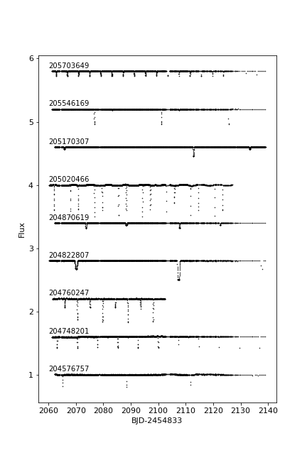
Figure 3: Light curves of long-period eclipsing binaries from Kepler campaign 2. The flux is measured relative to the median out-of-eclipse level and offset by multiple of 0.5 units for clarity. Trends in the data due to variations in spacecraft pointing have been removed.

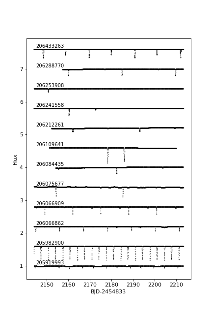
Figure 4: Light curves of long-period eclipsing binaries from Kepler campaign 3. The flux is measured relative to the median out-of-eclipse level and offset by multiple of 0.5 units for clarity. Trends in the data due to variations in spacecraft pointing have been removed.

2.3 WASP archive photometry

The WASP project has obtained over 580 billion photometric observations for more than 30 million bright stars during a survey that has discovered more than 150 transiting exoplanets since observations started in May 2004 (Pollacco et al. 2006). WASP photometry is available for many of the systems in Table 1, but is of much lower quality than the K2 photometry. Nevertheless, WASP photometry has enabled us to determine or refine the orbital period for long-period binaries where only two or three eclipses have been observed by the Kepler K2 mission.

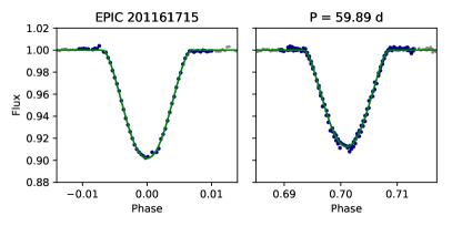
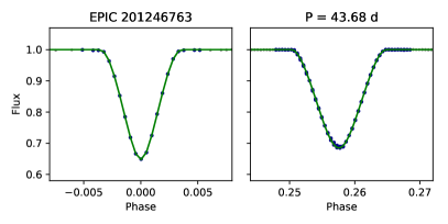
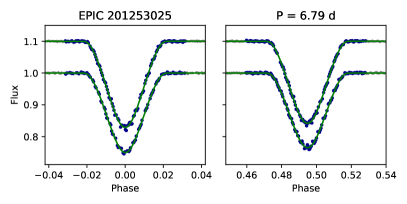
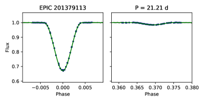
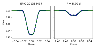
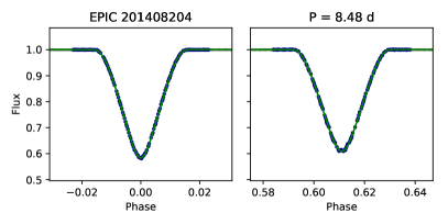
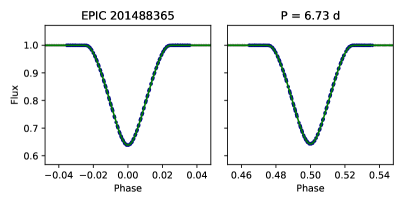
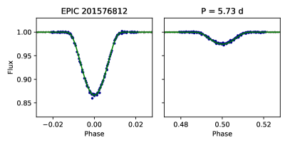
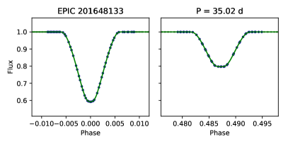
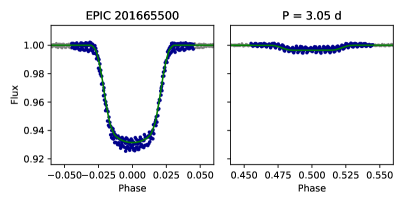
Figure 5: K2 light curves with the best-fit ellc model. Data not included in the fit are plotted using small grey points. Data obtained after BJD 2456849 for 201253025 are offset vertically by 0.1 flux units.

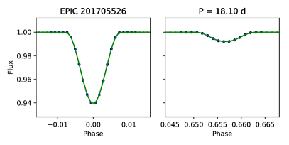
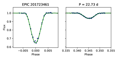
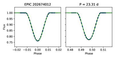
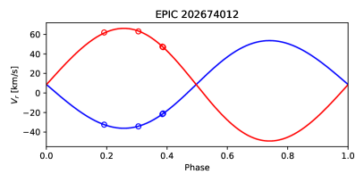
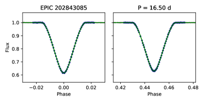
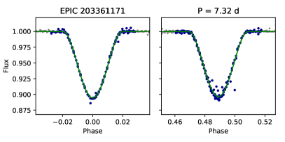
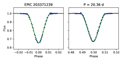
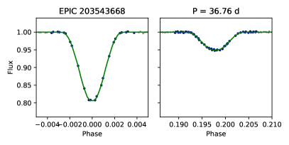
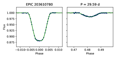
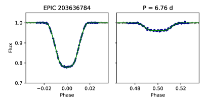
Figure 6: K2 light curves with the best-fit ellc model. Data not included in the fit are plotted using small grey points. For EPIC 202674012 we also show our best-fit Keplerian orbit to the measured radial velocities as a function of the orbital phase relative to the time of mid-primary eclipse.

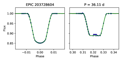
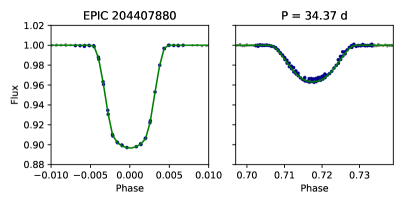
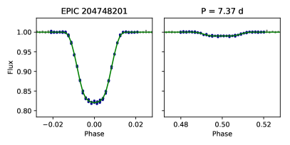
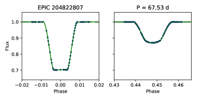
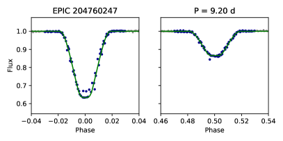
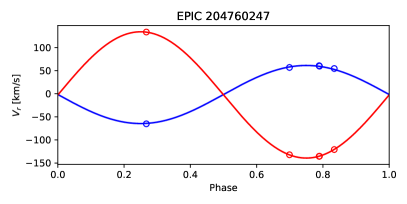
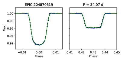
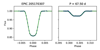
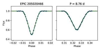
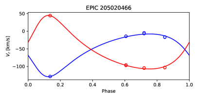
Figure 7: K2 light curves with the best-fit ellc model. Data not included in the fit are plotted using small grey points. For EPIC 204760247 and EPIC 205020466 we also show our best-fit Keplerian orbit to the measured radial velocities as a function of the orbital phase relative to the time of mid-primary eclipse.

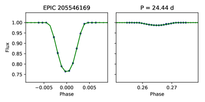
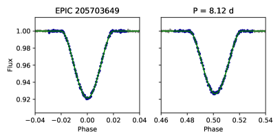
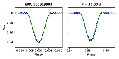
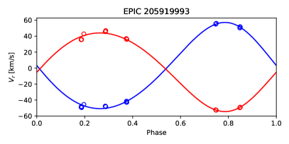
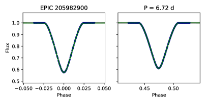
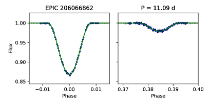
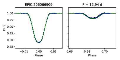
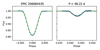
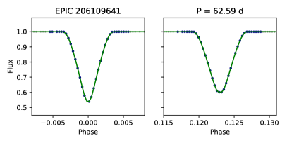
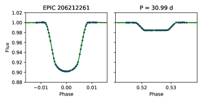
Figure 8: K2 light curves with the best-fit ellc model. Data not included in the fit are plotted using small grey points. For EPIC 205919993 we also show our best-fit Keplerian orbit to the measured radial velocities as a function of the orbital phase relative to the time of mid-primary eclipse.

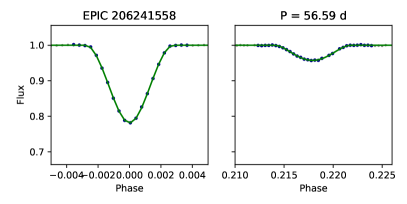
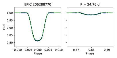
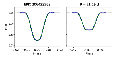
Figure 9: K2 light curves with the best-fit ellc model. Data not included in the fit are plotted using small grey points.

Table 1: Targets selected for further analysis from Kepler K2 campaigns 1, 2 and 3.

EPIC	C	Kp	$P$ [d]	$D_{1}$	$W_{1}$	$\phi_{2}$	$D_{2}$	$W_{2}$	Type	Notes
201160323	1	18.23	22.18	0.34	0.008	0.385	0.21	0.010	P	Rapid apsidal motion
201161715	1	14.65	59.89	0.10	0.014	0.701	0.09	0.016	P
201246763	1	11.93	43.68	0.35	0.008	0.258	0.31	0.014	P
201253025	1	12.86	6.79	0.26	0.042	0.494	0.24	0.046	P	$P_{\rm rot}=6.5,7.2$ d
201379113	1	14.76	21.21	0.34	0.009	0.369	0.02	0.011	P
201382417	1	11.66	5.20	0.07	0.048	0.500	0.01	0.048	T	$P_{\rm rot}=5.2$ d
201408204	1	11.85	8.48	0.42	0.031	0.611	0.39	0.036	T	$P_{\rm rot}=7.4,8.4$ d
201488365	1	8.81	6.73	0.36	0.048	0.500	0.36	0.048	P	FM Leo
201576812	1	10.07	5.73	0.15	0.028	0.500	0.05	0.028	P	TYC 272-458-1, $P_{\rm rot}=6.1$ d
201648133	1	10.14	35.02	0.41	0.012	0.487	0.21	0.011	T	Period constraint from WASP data
201665500	1	12.14	3.05	0.07	0.060	0.500	0.003	0.060	T	$P_{\rm rot}=3.2$ d
201705526	1	9.94	18.10	0.06	0.016	0.656	0.01	0.012	P	BD +04∘ 2479
201723461	1	14.91	22.73	0.34	0.009	0.345	0.06	0.010	P
202674012	2	9.77	23.31	0.24	0.022	0.497	0.22	0.021	P	HD 149946. FEROS spectra
202843085	2	11.80	16.50	0.38	0.030	0.448	0.38	0.034	P
203361171	2	11.92	7.32	0.11	0.038	0.489	0.11	0.038	P
203371239	2	11.74	20.36	0.35	0.025	0.500	0.35	0.022	P	Pulsations
203543668	2	13.68	36.76	0.20	0.005	0.198	0.05	0.012	P	$P_{\rm rot}=9.0$ d
203610780	2	12.24	29.60	0.12	0.012	0.482	0.02	0.017	T
203636784	2	12.87	6.76	0.25	0.036	0.500	0.05	0.036	T	$P_{\rm rot}=7.0$ d
203728604	2	10.56	36.11	0.15	0.018	0.321	0.12	0.024	T	$P_{\rm rot}=2.3$ d (pulsations?)
204407880	2	12.14	34.37	0.10	0.010	0.718	0.03	0.021	T	$P_{\rm rot}=13.3$ d
204576757	2	13.67	23.28	0.19	0.010	–	–	–	N
204748201	2	14.63	7.36	0.18	0.028	0.500	0.008	0.028	T
204760247	2	5.95	9.20	0.38	0.040	0.500	0.15	0.040	T	HD 142883. Pulsations. FEROS spectra
204822807	2	11.80	67.53	0.30	0.020	0.448	0.13	0.018	T
204870619	2	13.22	34.07	0.08	0.014	0.430	0.04	0.020	T
205020466	2	13.44	8.76	0.52	0.022	0.325	0.40	0.024	P	$P_{\rm rot}=6.7,5.7$ d, HRS spectra
205170307	2	12.28	67.50	0.14	0.008	0.304	0.03	0.009	T	$P_{\rm rot}=17$ d
205546169	2	11.66	24.44	0.24	0.009	0.265	0.01	0.014	P
205703649	2	12.49	8.12	0.08	0.040	0.500	0.07	0.040	P
205919993	3	10.14	11.00	0.06	0.012	0.552	0.06	0.013	P	LP 819-72, $P_{\rm rot}=13.4$ d
205982900	3	10.23	6.72	0.43	0.051	0.475	0.39	0.071	P	BW Aqr, pulsations
206066862	3	10.28	11.09	0.13	0.015	0.384	0.03	0.016	P	BD $-13^{\circ}$ 6219. $P_{\rm rot}=12.2$ d.
206066909	3	12.37	12.94	0.22	0.016	0.686	0.04	0.027	T
206075677	3	12.30	31.02	0.30	0.010	0.569	0.02	0.013	P	$P_{\rm rot}=9.3,4.3,7.7$ d. Triple?
206084435	3	14.65	48.22	0.19	0.008	0.443	0.04	0.009	P
206109641	3	12.38	62.59	0.46	0.008	0.123	0.40	0.008	T	Period from K2+WASP data
206212261	3	12.70	30.99	0.10	0.016	0.525	0.02	0.014	T
206241558	3	13.38	56.59	0.28	0.005	0.218	0.05	0.008	P	Period from K2+WASP data
206253908	3	11.18	65.45	0.10	0.005	–	–	–	N	Period from K2+WASP data
206288770	3	12.45	24.76	0.19	0.011	0.679	0.01	0.015	T
206433263	3	12.01	21.19	0.26	0.020	0.482	0.16	0.017	T

The two WASP instruments are located at the Observatorio del Roque de los Muchachos, La Palma and at Sutherland Observatory, South Africa. Both instruments carry an array of eight wide-field cameras, each with a 2048 $\times$ 2048 pixel CCD detector. The majority of the survey has been conducted using 200-mm, f/1.8 lenses combined with a filter that defines a bandpass covering the wavelengths 400-700 nm (Pollacco et al. 2006). From July 2012 the WASP-South instrument has used 85-mm, f/1.2 lenses with SDSS r^′ filters (Smith & WASP Consortium 2014). A dedicated pipeline is used to perform aperture photometry on the images at the position of catalogued stars within the images. The data are then processed by a detrending algorithm that has been developed from the SysRem algorithm of Tamuz et al. (2005), as described by Collier Cameron et al. (2006).

2.4 Light curve modeling

We used version 1.6.1 of the ellc light curve model (Maxted 2016) to determine the geometry and other parameters for each binary system. Note that the definition of the “third light” parameter used in this version of ellc to account for light from other stars in the photometric aperture is different to the one described in Maxted (2016). In the new version, third light is described by the parameter $\ell_{3}$. This parameter is used to calculate the flux ${\cal F}_{3}=\ell_{3}\left({\cal F}_{\rm N,1}+{\cal F}_{\rm N,2}\right)$, where ${\cal F}_{\rm N,1}$ is the flux from star 1 emitted towards star 2 and vice versa. This value of ${\cal F}_{3}$ is then used in the calculation of the observed flux ${\cal F}_{i}$ at time $t_{i}$ as before, i.e.,

$${\cal F}_{i}=\frac{{\cal F}_{i,1}+{\cal F}_{i,2}+{\cal F}_{3}}{{\cal F}_{\rm N,1}+{\cal F}_{\rm N,2}+{\cal F}_{3}},$$

where ${\cal F}_{i,1}$ is the flux emitted by star 1 towards the observer at time $t_{i}$ and similarly for ${\cal F}_{i,2}$. A complete list of changes in ellc version 1.6.1 is provided in the file CHANGELOG.rst provided with the package distribution.

The details of the analysis are not the same for every binary system because some binary systems have peculiarities that required special treatment. Here we outline the main features of the analysis applied to the majority of the systems analysed. Additional details and differences from this general approach for individual systems are described in Section 3.1.

The free parameters in the model for each binary were: the sum of radii of the stars in units of the semi-major axis – $r_{\rm sum}=(R_{1}+R_{2})/a$, the ratio of the radii – $k=R_{2}/R_{1}$; the surface brightness ratio in the Kepler band – $S_{\rm Kp}$; the orbital inclination, $i$; the time of primary eclipse – $T_{0}$; the orbital period – $P$; $f_{s}=\sqrt{e}\sin(\omega)$ and $f_{c}=\sqrt{e}\cos(\omega)$, where $e$ is the orbital eccentricity and $\omega$ is the longitude of periastron; and “third light” – $\ell_{3}$.

We use $f_{s}$ and $f_{c}$ as parameters because a uniform prior probability distribution for these parameters corresponds to a uniform prior probability distribution for $e$. We use a quadratic limb-darkening law for both stars with priors on the coefficients calculated using ldtk (Parviainen & Aigrain 2015) based on the spherical model atmospheres by Husser et al. (2013). To calculate these priors we assume $\log g=4.3\pm 0.3$ and [Fe/H]$=0.0\pm 0.2$ for all stars and effective temperature estimates from a preliminary analysis very similar to those derived in below in Section 2.5. The standard error estimates on the coefficients inherited from the assumed errors on T_eff, $\log g$ and [Fe/H] are likely to be underestimates of the true uncertainties since they do not account for systematic errors in the models and other issues with estimating limb darkening coefficients from models (Howarth 2011). To allow for this additional uncertainty we add 0.05 in quadrature to the standard error estimates for both coefficients. This estimate of the systematic error in the coefficients dominates the error budget for the limb darkening so we did not consider it necessary to re-calculate these coefficients for the slightly different values of $T_{\rm eff}$ derived in Section 2.5 cf. our preliminary solution. Rather than sampling the limb darkening coefficients $u_{1}$ and $u_{2}$ directly, we use the parameters $q_{1}=(u_{1}+u_{2})^{2}$ and $q_{2}=0.5u_{1}/(u_{1}+u_{2})$ since this makes it easier to uniformly sample the allowed parameter space (Kipping 2013). Unless otherwise noted, we used spheres to model the shape of these well-detached stars so gravity darkening was ignored. There is little or no information about the geometry of the binary system in the observations between the eclipses. For the light curve modeling of most stars we used only observations over a range 1.5 times the full eclipse width centered on each eclipse. This had the advantage of speeding up the calculation. We used numerical integration of the eclipse model to account for the exposure time of 1765 s for data obtained near or during an eclipse.

It is notoriously difficult to include star spots in the model for an eclipsing binary star because the number of free parameters required is large and the constraints on these parameters from the light curve are generally weak and highly degenerate. We did not attempt to model star spots for any of the binary systems here since the amplitude of the star spot modulation is generally quite small ($\la 0.5\%$) so the resulting systematic error in the parameters derived will, in general, not be large enough to alter our conclusions regarding the nature of the binary. Instead, we simply divide-out the time trend due to star spot modulation established from the Gaussian process fit to the out-of-eclipse data.

We used emcee (Foreman-Mackey et al. 2013), a python implementation of an affine invariant Markov chain Monte Carlo (MCMC) ensemble sampler, to calculate the posterior probability distribution of the model parameters. We used an ensemble with at least twice the number samples per chain step (“walkers”) as there were model parameters and 5,000 or 10,000 steps in the chain used for the results quoted below. The convergence of the chain was judged by visual inspection of the parameters and the likelihood as a function of step number. In cases where we suspected the chain had not sampled the posterior probability distribution accurately we calculated a new Markov Chain starting from the best-fit parameters in the previous chain and using an increased number of chain steps and/or an increased number of walkers with a large spread of initial parameter values to ensure convergence. The standard error per observation was either assumed to be constant for all the data, or assumed to be constant within each of two blocks of data where there is a gap in the observations. These values of the standard error were included as free parameters in the MCMC analysis by including the necessary term in the calculation of the likelihood for each chain step. Unless otherwise stated, we only use data within a range of 1.5 times the eclipse width (as listed in Table 1) centred on each eclipse in this analysis. This ensures that these standard error estimates (and, hence, the error estimates on the model parameters) are determined by the scatter in the residuals through the eclipse, rather than the much lower scatter in the residuals between the eclipses. From preliminary fits to the complete light curves we found that the out-of-eclipse level is always very close to the value 1 with a very small error and is not correlated with the other parameters so we fix this parameter at 1 for the analysis presented here.

The aim of this analysis is to characterise each binary system in order to identify systems of interest for further study and for comparison to binary population models. The parameters we have derived are reliable enough for this purpose but further work is needed to determine the accuracy of these parameters. The K2 data clearly have the potential to produce very precise parameters for some binary systems, but we have not attempted to characterise the level of systematic error in these parameters for all the systems studied. We advise that a careful study of these issues should be done before the parameters of individual binary systems are used to test stellar evolution models.

2.5 Effective temperature estimates

We have used empirical colour – effective temperature and colour – surface brightness relations to estimate the effective temperatures of the individual stars in the binary and triple systems we have studied. We extracted photometry for each target from the following catalogues – B_T and V_T magnitudes from the Tycho-2 catalogue (Høg et al. 2000); B, V, g^′, r^′ and i^′ magnitudes from data release 9 of the AAVSO Photometric All Sky Survey (APASS9, Henden et al. 2016); J, H and K_s magnitudes from the Two-micron All Sky Survey (2MASS, Skrutskie et al. 2006); i^′, J and K magnitudes from the Deep Near-infrared Southern Sky Survey (DENIS, The DENIS Consortium 2005). Not all stars have data in all these catalogues. Photometry from the Sloan digital sky survey (SDSS) can be unreliable for these bright stars because they saturate the detectors, but we have used g^′-, r^′- and i^′-band “psfMag” magnitudes from data release 9 of the SDSS (Ahn et al. 2012) in some cases, as noted in Table 2.5. Magnitudes from the APASS9 catalogue that are given with a standard error estimate of 0.00 were not included in our analysis.

longtablelrrrrrrrrrr Effective temperature estimates from empirical colour – effective temperature and colour – surface brightness relations and constraints from the K2 light curve analysis.
EPIC g${}^{\prime}_{0,1}$ T_eff,1 g${}^{\prime}_{0,2}$ T_eff,2 g${}^{\prime}_{0,3}$ T_eff,3 E$({\rm B}-{\rm V})$ $\sigma_{\rm ext}$ $N_{\rm mag}$
[mag] [K] [mag] [K] [mag] [K] [mag]
continued.
EPIC g${}^{\prime}_{0,1}$ T_eff,1 g${}^{\prime}_{0,2}$ T_eff,2 g${}^{\prime}_{0,3}$ T_eff,3 E$({\rm B}-{\rm V})$ $\sigma_{\rm ext}$ $N_{\rm mag}$
[mag] [K] [mag] [K] [mag] [K] [mag]
201161715  15.36 5030 17.15 5370 0.034 0.019 14
$\pm$ 0.10 85 0.21 120 0.025
201246763 13.23 5875 12.66 6225 0.026 0.000 11
$\pm$ 0.10 110 0.09 125 0.024
201253025 13.82 6065 13.92 6070 0.031 0.009 9
$\pm$ 0.17 155 0.18 155 0.023
201379113  15.25 5150 19.9 3900 0.039 0.030 14
$\pm$ 0.12 115 1.6 230 0.028
201382417 13.29 6175 17.08 4480 12.54 4950 0.055 0.035 12
$\pm$ 0.16 400 0.16 200 0.14 140 0.030
201408204 12.84 5845 12.94 5830 0.030 0.002 10
$\pm$ 0.09 105 0.09 100 0.024
201488365  9.21 6355 9.40 6345 0.023 0.004 10
$\pm$ 0.10 150 0.10 150 0.024
201576812 10.49 5905 13.1 4360 0.037 0.061 13
$\pm$ 0.11 190 0.5 140 0.023
201648133 10.65 6010 12.32 5250 0.028 0.020 11
$\pm$ 0.07 95 0.07 70 0.019
201665500 12.30 6270 19.4 3630 0.028 0.001 9
$\pm$ 0.09 120 0.9 60 0.022
201705526 11.71 6600 15.93 4320 10.24 6020 0.033 0.048 11
$\pm$ 0.15 430 0.16 195 0.11 170 0.024
201723461  16.26 4450 17.0 4170 0.050 0.023 12
$\pm$ 0.23 140 0.4 160 0.030
202674012  10.0 6250 11.3 6150 0.096 0.058 11
$\pm$ 0.2 285 0.2 285 0.065
202843085 12.4 6300 12.2 6260 0.172 0.002 12
$\pm$ 0.2 280 0.2 280 0.060
203361171 12.4 6070 12.3 6050 0.148 0.009 14
$\pm$ 0.3 290 0.3 280 0.064
203371239 11.6 6400 12.0 6300 16.3 3660 0.378 0.019 9
$\pm$ 0.3 380 0.3 380 0.7 335 0.084
203543668 14.2 5900 16.8 4600 13.92 5300 0.267 0.002 11
$\pm$ 0.3 550 0.3 315 0.25 310 0.066
203610780 14.2 6650 13.4 5600 13.3 5700 0.058 0.055 8
$\pm$ 0.3 350 0.3 300 1.1 725 0.048
203636784 13.02 5970 17.1 4350 0.099 0.032 9
$\pm$ 0.17 200 0.2 100 0.044
203728604  10.98 6050 13.27 5840 0.019 0.018 11
$\pm$ 0.07 100 0.07 95 0.019
204407880 12.1 5765 15.7 4900 0.188 0.004 14
$\pm$ 0.2 205 0.2 145 0.054
204748201 14.7 6100 20.8 3600 17.1 5400 0.168 0.027 8
$\pm$ 0.2 235 0.2 110 0.6 1100 0.050
204822807  13.3 5625 12.9 4620 15.3 4665 0.087 0.016 12
$\pm$ 0.2 215 0.2 135 0.9 350 0.055
204870619 13.3 5435 17.0 4800 0.162 0.005 12
$\pm$ 0.3 250 0.3 190 0.070
205020466 13.3 5300 13.7 5070 0.670 0.021 9
$\pm$ 0.5 480 0.5 425 0.145
205170307  12.49 5620 16.79 4240 16.1 4490 0.126 0.003 9
$\pm$ 0.08 65 0.09 40 0.2 90 0.022
205546169  13.1 6300 12.0 6170 16.1 5050 0.100 0.003 14
$\pm$ 0.2 210 0.2 210 1.0 500 0.045
205703649 12.9 5610 12.8 5540 0.256 0.000 8
$\pm$ 0.4 425 0.4 415 0.103
205919993 12.2 4025 11.8 4230 0.027 0.077 10
$\pm$ 0.1 60 0.1 60 0.021
205982900  11.49 6200 11.21 6045 0.011 0.070 11
$\pm$ 0.07 115 0.07 110 0.013
206066862  10.8 6250 12.4 5000 0.043 0.048 11
$\pm$ 0.2 300 0.7 200 0.032
206066909 12.91 6440 16.66 4535 13.95 5225 0.057 0.020 9
$\pm$ 0.13 290 0.12 140 0.19 360 0.031
206084435 14.91 5950 18.91 4300 0.042 0.001 8
$\pm$ 0.11 135 0.15 140 0.030
206109641  13.18 5905 13.65 5805 0.034 0.001 11
$\pm$ 0.10 120 0.10 115 0.025
206212261 13.15 5385 18.24 4010 0.028 0.001 14
$\pm$ 0.09 85 0.09 50 0.023
206241558 14.31 5330 14.74 5885 0.052 0.006 9
$\pm$ 0.15 120 0.21 160 0.031
206288770 12.45 6290 18.02 3870 0.078 0.007 12
$\pm$ 0.09 120 0.09 55 0.024
206433263 12.52 6000 14.46 5525 0.034 0.018 14
$\pm$ 0.08 90 0.08 75 0.020

Our model for the observed photometry then has the following free parameters that are determined by a least-squares fit to the observed apparent magnitudes and other data for each system – g${}^{\prime}_{0,i}$, the apparent g^′-band magnitudes for stars $i=1$, $i=2$ and (for triple systems) $i=3$, corrected for extinction; $T_{\rm eff,i}$ the effective temperatures for each star in the binary or triple system; E$({\rm B}-{\rm V})$, the reddening to the system; $\sigma_{\rm ext}$ the additional systematic error added in quadrature to each synthetic magnitude to account for systematic errors in the conversion to observed magnitudes.

For each trial combination of these parameters we use the empirical colour – effective temperature relations by Boyajian et al. (2013) to predict the apparent magnitudes for each star in each of the observed bands. We used the same transformation between the Johnson and 2MASS photometric systems as Boyajian et al.. We used the Cousins I_C band as an approximation to the DENIS Gunn i^′ band and the 2MASS K_s band as an approximation to the DENIS K band (see Fig. 4 Bessell 2005). We used interpolation in Table 3 of Bessell (2000) to transform the Johnson B, V magnitudes to Tycho-2 B_T and V_T magnitudes. We assume that the extinction in the V band is $3.1\times{\rm E}({\rm B}-{\rm V})$. Extinction in the SDSS and 2MASS bands is calculated using A${}_{\rm r}=2.770\times{\rm E}({\rm B}-{\rm V})$ from Fiorucci & Munari (2003) and extinction coefficients relative to the r^′ band from Davenport et al. (2014).

We use the transformation from Sloan g^′, r^′ and i^′ magnitudes by Brown et al. (2011) to estimate Kepler Kp magnitudes for each star in the system. This enables us to include the flux ratio $\ell_{\rm Kp}$ as a constraint in the analysis of the published photometry. Another useful constraint is the surface brightness ratio in the Kepler band, $S_{\rm Kp}$, which we account for by using the empirical relation between the V-band surface brightness $S_{\rm V}$ and $(\rm B-\rm K)$ from Graczyk et al. (2017). The comparison between the predicted and observed values is done in terms of the surface brightness parameter

$$S_{i}=m_{i,0}+5\log\phi,$$

where $i$ denotes a particular band (V or Kp), $\phi$ is the angular diameter in milli-arcseconds, and $m_{i,0}$ is the de-reddened apparent magnitude in a given band, so that $S_{\rm Kp}=S_{\rm V}+({\rm Kp}-{\rm V})$.

We used emcee (Foreman-Mackey et al. 2013) to sample the posterior probability distribution for our model parameters. We used the reddening maps by Schlafly & Finkbeiner (2011) to estimate the total line-of-sight extinction to each target, ${\rm E}({\rm B}-{\rm V})_{\rm map}$. This value is used to impose the following (unnormalized) prior on $\Delta={\rm E}({\rm B}-{\rm V})-{\rm E}({\rm B}-{\rm V})_{\rm map}$:

$$P(\Delta)=\left\{\begin{array}[]{ll}1&\Delta\leq 0\\ \exp(-0.5(\Delta/0.034)^{2})&\Delta>0\\ \end{array}\right.$$

The constant 0.034 is taken from Maxted et al. (2014) and is based on a comparison of ${\rm E}({\rm B}-{\rm V})_{\rm map}$ to ${\rm E}({\rm B}-{\rm V})$ from Strömgren photometry for 150 A-type stars. A least-squares optimisation algorithm was used to find an initial set of parameters for the chain and the Markov chains were calculated using 64 walkers and 256 steps following a burn-in run of 128 steps. An example of the output from the program used to implement our method is shown in Fig. 10.

Read 17 lines from EPIC201161715.phot

 Calculating least-squares solution...
  g_1     = 15.50
  T_eff,1 = 4931 K
  g_2     = 17.25
  T_eff,2 = 5264 K
  E(B-V)  =   0.00
  chi-squared = 3.44
  Ndf = 12
  sigma_ext = 0.05

 Starting emcee chain of 384 steps with 64 walkers

 Median acceptance fraction = 0.487
 Best log(likelihood) = 42.52 in walker 12 at step 155

 Parameter median values, standard deviations and best-fit values.
  g_1     = 15.362 +/-  0.102   [ 15.460 ]
  T_eff,1 =   5031 +/-   84 K     [ 4958 ]
  g_2     = 17.148 +/-  0.207   [ 17.231 ]
  T_eff,2 =   5366 +/-  120 K     [ 5282 ]
  E(B-V)  =  0.034 +/-  0.025   [  0.011 ]
  sig_ext =  0.027 +/-  0.016   [  0.019 ]
  chi-squared = 9.90

type band value_obs error   source  value_fit value_A  value_B   z
---- ---- --------- ------ -------- --------- -------- -------- ----
 mag    B    15.759  0.208   APASS9   15.7578  15.9591  17.6869 0.01
 mag    H    12.769  0.021    2MASS   12.8287  12.9722  15.0962 2.11
 mag   Ic    13.916   0.03    DENIS   13.9310  14.0947  16.0660 0.42
 mag    J    13.227   0.07    DENIS   13.2451  13.3976  15.4518 0.25
 mag    J    13.283  0.027    2MASS   13.2451  13.3976  15.4518 1.15
 rat  K_p      0.18   0.03 paper-v3    0.1771  14.8825  16.7617 0.10
 sb2  K_p       1.4    0.1 paper-v3    1.3832   5.3211   4.9689 0.17
 mag   Ks    12.602   0.14    DENIS   12.6763  12.8175  14.9610 0.53
 mag   Ks    12.725   0.03    2MASS   12.6763  12.8175  14.9610 1.37
 mag    V    14.881  0.024   APASS9   14.8917  15.0734  16.9224 0.35
 mag    g   15.2956  0.019     SDSS   15.3090  15.5032  17.2736 0.50
 mag    g    15.259   0.11   APASS9   15.3090  15.5032  17.2736 0.45
 mag    i    14.413   0.05   APASS9   14.3643  14.5308  16.4828 0.91
 mag    i   14.3639 0.0192     SDSS   14.3643  14.5308  16.4828 0.02
 mag    r    14.581  0.103   APASS9   14.5961  14.7691  16.6755 0.14
 mag    r   14.6083 0.0133     SDSS   14.5961  14.7691  16.6755 0.53
 Nobs = 17
 Nmag = 14
 Ndf  = 11
 BIC = -68.04

Completed analysis of EPIC201161715.phot

Figure 10: Example output from our program to estimate T_eff for the stars in an eclipsing binary from a least-squares fit to the observed apparent magnitudes and other constraints.

There will be some systematic error in the T_eff estimates for stars in eclipsing binaries cooler than 4900 K because we have extrapolated the empirical $S_{\rm V}$ – $(\rm B-\rm K)$ relation in this regime. The empirical colour – temperature relations we have used are valid over the approximate range T${}_{\rm eff}=3450$ K to 8600 K. Our results may be biased in systems where one of the stars has an effective temperature near either of these limits because we exclude trial solutions with any T_eff,i value outside this range. Between these limits we use uniform priors on the values of T_eff,i. We also use uniform priors for g${}^{\prime}_{0,1}$ and g${}^{\prime}_{0,2}$.

In systems where there is evidence of third light from the light curve analysis and the star appears unresolved in sky survey images we compare solutions with a uniform prior on g${}^{\prime}_{0,3}$ and with a constraint on g^′_0,3 assuming that the third light is due to a main-sequence star at the same distance as the eclipsing binary star. We use the stellar model from the Dartmouth stellar evolution database (Dotter et al. 2008) for solar composition to define the limits of the main sequence in the T_eff – $M_{\rm g^{\prime}}$ plane, where $M_{\rm g^{\prime}}$ is the absolute magnitude of star $i$ in the g^′ band. For each trial solution we use interpolation between these model isochrones to define limits to g${}^{\prime}_{0,3}$ assuming that the fainter star in the eclipsing binary is a main-sequence star, i.e., we reject solutions where the combination of T_eff,3, T_eff,B, g${}^{\prime}_{0,3}$ and g${}^{\prime}_{0,B}$ cannot be reproduced by two stars between the zero-age main sequence and terminal-age main-sequence in the T_eff – $M_{{\rm g}^{\prime}}$ plane, where $B=1$ or 2 is the index for the star in the eclipsing binary that is fainter in the g^′-band. Systems where we adopted solutions including this constraint are noted with a $\star$ symbol in Table 2.5, together with the median and standard deviation of the model parameters derived using emcee.

Our method requires an estimate of the apparent g^′ magnitude. In cases where no such estimate is available from APASS9 we either use the SDSS g^′ magnitude or infer a value from the Tycho-2 B_T and V_T magnitudes using equation (6a) from Brown et al. (2011). In either case, we assign an nominal standard error of 0.5 magnitudes to this estimate. We also found for some stars that the magnitudes from the DENIS and 2MASS surveys were significantly different. In general, we used the 2MASS magnitudes in these cases and excluded the DENIS photometry from the fit – these cases are noted in Table 2.5.

3 Results

The parameters derived from our analysis of the K2 light curves for each target are given in Tables 2 and 3. The best fits to the K2 light curves are shown in Figs. 5, 6, 7 and 8. The effective temperature estimates for the components of each system are given in Table 2.5. In Table 4 we give an estimate of the mean stellar density ($\rho_{\star}$) for the two stars in each eclipsing binary calculated using the following expression derived from Kepler’s third law.

$$\mbox{$\rho_{\star}$}=\frac{3\mbox{M${}_{\star}$}}{4\pi R_{\star}^{3}}=\frac{3\pi}{GP^{2}(1+q)}\left(\frac{a}{\mbox{R${}_{\star}$}}\right)^{3}.$$

Here, $P$ and $a$ are the period and semi-major axis of the Keplerian orbit, and $q=M_{\mathrm{c}}/\mbox{$M_{\star}$}$ is the mass ratio for a companion with mass $M_{\mathrm{c}}$ to a star with mass $M_{\star}$ and radius $R_{\star}$. The value of $q$ was estimated by calculating the position of the stars in Fig. 11 for various values of $q$ and then choosing the value which is consistent with the approximate masses inferred from the stellar evolution tracks shown in this figure.

Table 2: Geometric and orbital parameters derived from the analysis of the K2 light curves for selected long-period eclipsing binary stars.

EPIC	$(R_{1}+R_{2})/a$	$R_{2}/R_{1}$	$i$ [∘]	$T_{0}$	$P$	$f_{c}$	$f_{s}$
201160323	0.0276(2)	1.10(6)	89.80(5)	2023.026(1)	22.200(6)	$-0.406(2)$	$0.19(1)$
201161715	0.061(1)	0.36(1)	87.64(8)	2007.4140(9)	59.887(2)	$0.542(4)$	$0.22(2)$
201246763	0.0351(1)	1.13(2)	89.40(1)	2014.32552(9)	=43.68281(3)	$-0.504(1)$	$0.514(3)$
201253025	0.1418(7)	1.0(1)	87.4(2)	2011.3371(3)	6.78651(9)	$-0.038(2)$	$0.21(1)$
	0.1425(8)	0.95(8)	87.3(2)	2011.3367(3)	6.78635(8)	$-0.038(2)$	$0.21(1)$
201379113	0.037(2)	0.8(1)	88.7(1)	1989.2348(2)	21.2146(1)	$-0.3(1)$	$0.5(1)$
201382417	0.1350(5)	0.51(1)	88.8(2)	1983.27151(7)	5.197721(9)	$-0.008(4)$	$0.01(3)$
201408204	0.1067(2)	0.97(2)	88.95(1)	2002.45835(4)	8.48185(1)	$0.388(1)$	$0.226(5)$
201488365	0.1518(1)	0.917(6)	87.96(1)	2019.59540(1)	6.728609(3)	$0.005(2)$	$0.010(9)$
201576812	0.106(3)	0.9(2)	85.7(3)	2015.96974(7)	5.72830(2)	$0.001(2)$	$0.11(8)$
201648133	0.03513(1)	0.687(2)	89.734(4)	2015.81404(1)	=35.02402(1)	$-0.0941(8)$	$-0.192(2)$
201665500	0.171(1)	0.2474(9)	89.9(5)	2017.2344(1)	3.05351(2)	$-0.00(2)$	$0.03(6)$
201705526	0.0436(3)	0.599(8)	89.24(4)	2004.71250(3)	=18.102928	$0.476(2)$	$-0.206(7)$
201723461	0.04(1)	1.1(3)	88(1)	1997.146(2)	22.731(1)	$-0.7(2)$	$0.3(2)$
202674012	0.0718(1)	0.562(2)	88.65(1)	2076.36053(5)	23.30962(5)	$-0.0295(9)$	$-0.162(5)$
202843085	0.1057(2)	1.16(1)	88.84(2)	2077.35748(9)	16.49843(5)	$-0.259(2)$	$0.184(6)$
203361171	0.148(6)	1.1(2)	85.0(7)	2068.8147(8)	7.3216(2)	$-0.130(8)$	$-0.02(4)$
203371239	0.0730(4)	0.88(5)	88.98(7)	2078.9883(3)	20.3618(3)	$-0.0034(3)$	$-0.20(1)$
203543668	0.0278(3)	0.68(2)	89.7(2)	2099.4015(3)	36.7623(4)	$-0.583(4)$	$0.516(9)$
203610780	0.0584(8)	2.37(3)	88.12(5)	2082.5913(2)	29.5937(5)	$-0.044(1)$	$0.61(1)$
203636784	0.1140(7)	0.461(9)	89.1(2)	2066.5457(2)	6.76465(4)	$0.000(1)$	$0.15(2)$
203728604	0.0664(1)	0.385(2)	89.71(9)	2066.85857(7)	36.108(1)	$-0.5084(4)$	$0.221(2)$
204407880	0.0542(6)	0.316(5)	88.56(5)	2084.7125(1)	34.36789(2)	$0.389(4)$	$0.664(7)$
204748201	0.0839(6)	0.43(1)	89.6(3)	2070.5201(1)	7.36575(4)	$0.00(1)$	$0.00(5)$
204760247	0.114(1)	0.65(1)	90.0(4)	2079.7559(8)	9.2022(6)	$0.007(8)$	$0.01(5)$
204822807	0.05558(7)	2.38(1)	89.88(9)	2107.3994(1)	67.535(1)	$-0.2837(3)$	$0.051(3)$
204870619	0.0517(2)	0.281(4)	89.9(2)	2073.7038(2)	34.0690(3)	$-0.217(1)$	$0.444(3)$
205020466	0.0792(2)	0.97(2)	89.98(9)	2067.9683(2)	8.75903(3)	$-0.467(2)$	$0.35(2)$
205170307	0.0270(2)	0.39(1)	89.51(4)	2112.8240(1)	67.5025(8)	$-0.5449(8)$	$0.177(5)$
205546169	0.0529(6)	1.74(2)	87.98(2)	2125.59047(8)	24.43581(6)	$-0.393(4)$	$0.696(6)$
205703649	0.152(3)	1.1(2)	84.7(3)	2083.1227(2)	8.11699(5)	$0.038(7)$	$-0.05(2)$
205919993	0.0530(3)	0.97(3)	87.69(1)	2182.4928(2)	11.00009(6)	$0.273(3)$	$0.12(2)$
205982900	0.1787(1)	1.196(5)	88.68(2)	2157.46696(2)	6.719684(4)	$-0.0942(2)$	$0.411(1)$
206066862	0.069(1)	0.74(9)	87.01(9)	2155.9185(1)	11.08666(5)	$-0.401(8)$	$0.21(3)$
206066909	0.0659(2)	0.567(6)	89.20(4)	2174.94439(3)	12.93712(2)	$0.454(1)$	$0.438(3)$
206084435	0.0278(4)	0.47(2)	89.30(4)	2182.3183(2)	48.221(2)	$-0.2989(3)$	$0.01(2)$
206109641	0.02915(1)	0.846(2)	89.98(2)	2178.17503(2)	62.58668(6)	$-0.79828(5)$	$0.047(1)$
206212261	0.0487(2)	0.302(5)	89.7(1)	2162.0314(1)	30.9857(2)	$0.133(1)$	$-0.260(4)$
206241558	0.0311(3)	0.63(4)	88.66(1)	2160.2622(1)	56.58934(5)	$-0.547(4)$	$0.536(8)$
206288770	0.0404(3)	0.415(4)	89.37(4)	2160.03956(6)	24.75656(5)	$0.477(3)$	$0.342(8)$
206433263	0.06039(4)	0.522(2)	89.33(1)	2169.57164(4)	21.19385(3)	$-0.0922(6)$	$-0.299(2)$

Table 3: Radiative parameters and other parameters of interest derived from the analysis of the K2 light curves for selected long-period eclipsing binary stars.

EPIC	$S_{\rm Kp}$	$\ell_{3}$	$\ell_{\rm Kp}$	$R_{1}/a$	$R_{2}/a$	$e$	$\omega$ [∘]	$\sigma$ [ppt]
201160323	0.62(1)	0.43(5)	0.75(7)	0.0132(4)	0.0145(3)	0.202(3)	154(2)	6.2, 4.8
201161715	1.4(1)	0.01(3)	0.18(3)	0.0446(6)	0.0161(6)	0.345(4)	23(2)	1.4, 2.7
201246763	1.23(2)	0.006(6)	1.58(4)	0.0165(2)	0.0186(1)	0.519(2)	134.4(2)	0.8, 2.5
201253025	1.00(1)	0.27(5)	1.0(2)	0.071(3)	0.071(3)	0.045(5)	100(1)	3.2
	1.01(1)	0.16(5)	0.9(2)	0.073(3)	0.070(3)	0.045(5)	100(1)	3.5
201379113	0.20(9)	=0	0.1(1)	0.021(2)	0.016(1)	0.35(4)	124(14)	2.6, 0.5
201382417	0.210(2)	2.8(2)	0.055(3)	0.0893(9)	0.0457(6)	0.001(1)	150(65)	0.4, 0.4
201408204	0.991(8)	0.004(4)	0.92(2)	0.0543(4)	0.0524(4)	0.202(1)	30.3(7)	1.2, 1.5
201488365	0.9945(7)	0.0005(8)	0.84(1)	0.0792(2)	0.0726(3)	0.0001(2)	–	0.5, 0.4
201576812	0.21(4)	=0	0.19(6)	0.055(4)	0.050(7)	0.01(2)	–	1.9, 0.9
201648133	0.542(2)	0.006(3)	0.2563(8)	0.02082(2)	0.01431(2)	0.0458(8)	243.9(5)	0.1, 0.3
201665500	0.059(2)	=0	0.0036(1)	0.137(1)	0.0339(3)	0.002(7)	–	2.7, 1.1
201705526	0.128(2)	4.5(2)	0.046(1)	0.0273(2)	0.0163(2)	0.269(2)	336.6(8)	0.1, 0.1
201723461	0.4(4)	=0	0.6(5)	0.017(7)	0.020(5)	0.6(2)	152(15)	24, 22
202674012	0.966(3)	0.005(5)	0.306(2)	0.04596(8)	0.0258(1)	0.027(2)	259.7(6)	0.3,0.4
202843085	0.970(6)	0.015(4)	1.30(3)	0.0490(4)	0.0567(3)	0.101(1)	144(1)	1.0, 1.3
203361171	0.98(4)	0.3(3)	1.2(4)	0.069(6)	0.079(5)	0.018(3)	189(18)	4.2, 3.6
203371239	0.94(1)	0.05(2)	0.73(8)	0.0388(9)	0.034(1)	0.039(5)	269.0(2)	2.7, 7.9
203543668	0.30(1)	1.4(1)	0.137(5)	0.0166(3)	0.0112(2)	0.606(4)	139(1)	1.3, 1.2
203610780	0.51(6)	1.2(2)	2.9(3)	0.0173(3)	0.0411(5)	0.37(1)	94.1(2)	0.8, 1.0
203636784	0.195(3)	0.05(4)	0.041(2)	0.0780(8)	0.0360(5)	0.021(6)	89.8(5)	2.1, 1.8
203728604	0.860(3)	0.012(8)	0.127(1)	0.0480(1)	0.01846(6)	0.3072(4)	156.5(2)	0.2, 2.4
204407880	0.46(2)	0.05(3)	0.047(2)	0.0412(5)	0.0130(2)	0.592(6)	59.6(5)	0.4, 1.8
204748201	0.063(2)	0.16(6)	0.0115(7)	0.0588(8)	0.0250(4)	0.001(3)	–	1.4, 1.8
204760247	0.389(6)	0.06(4)	0.167(8)	0.0689(7)	0.0451(9)	0.001(3)	–	8.7
204822807	0.364(2)	0.096(9)	2.06(3)	0.01644(7)	0.03914(9)	0.0831(2)	169.7(7)	0.5, 0.4
204870619	0.528(4)	0.05(2)	0.0417(9)	0.0403(2)	0.0113(1)	0.244(2)	116.1(2)	0.5, 0.7
205020466	0.79(1)	0.03(2)	0.74(2)	0.0402(3)	0.0390(4)	0.34(1)	143(2)	2.8, 2.6
205170307	0.219(1)	0.17(5)	0.034(2)	0.0193(2)	0.0076(1)	0.3282(8)	162.0(5)	0.3, 0.5
205546169	0.95(7)	0.09(5)	2.9(2)	0.0193(3)	0.0336(3)	0.639(6)	119.4(5)	0.5, 0.3
205703649	0.94(2)	0.8(2)	1.2(4)	0.071(5)	0.081(5)	0.004(2)	310(34)	0.8, 0.8
205919993	1.35(7)	=0	=1.28(5)	0.0269(5)	0.0261(4)	0.088(2)	24(3)	1.0, 0.9
205982900	0.929(3)	=0	1.329(6)	0.0814(2)	0.0974(1)	0.1775(8)	102.92(6)	0.5, 0.4
206066862	0.36(6)	=0	0.20(5)	0.040(2)	0.029(2)	0.205(8)	152(4)	1.2
206066909	0.189(2)	0.52(2)	0.0606(9)	0.0420(3)	0.0238(1)	0.398(2)	44.0(3)	0.45
206084435	0.200(2)	0.04(4)	0.044(4)	0.0189(2)	0.0089(3)	0.0896(2)	177(2)	1.0
206109641	0.932(3)	0.0008(7)	0.6664(9)	0.01579(2)	0.01336(1)	0.63944(3)	176.65(9)	0.20
206212261	0.185(1)	0.08(4)	0.0169(6)	0.0374(3)	0.0113(1)	0.085(2)	297.1(6)	0.3
206241558	1.6(1)	=0	0.6(1)	0.0191(4)	0.0120(5)	0.587(4)	135.6(7)	0.8
206288770	0.0804(7)	0.02(2)	0.0138(2)	0.0286(2)	0.01186(8)	0.345(3)	35.6(8)	0.4
206433263	0.691(3)	0.008(7)	0.188(1)	0.03967(6)	0.02072(6)	0.098(1)	252.8(2)	0.4

Table 4: Mean stellar densities, $\rho_{1}$ and $\rho_{2}$ calculated assuming a mass ratio $q=M_{2}/M_{1}$.

EPIC	$P$ [d]	Teff,1   [K]	$\log(\rho_{1}/\rho_{\odot})$		EPIC	$P$ [d]	Teff,1   [K]	$\log(\rho_{1}/\rho_{\odot})$
Symbol	$q$	Teff,2   [K]	$\log(\rho_{2}/\rho_{\odot})$		Symbol	$q$	Teff,2   [K]	$\log(\rho_{2}/\rho_{\odot})$
201253025	6.79	6065	$-0.4$		201408204	8.48	5845	$-0.2$
$\diamond$	1.0	6070	$-0.4$		$\circ$	1.0	5830	$-0.2$
201382417	5.20	6175	$-0.4$		201705526	18.10	6600	$0.1$
$\star$	0.6	4480	$0.3$		$\triangle$	0.5	4320	$0.5$
201488365	6.73	6355	$-0.5$		202843085	16.50	6300	$-0.7$
$\circ$	0.976	6345	$-0.4$		$\square$	1.0	6260	$-0.9$
201576812	5.73	5905	$0.2$		203371239	20.36	6400	$-0.6$
$\triangle$	0.66	4360	$0.1$		$\times$	1.0	6300	$-0.4$
201665500	3.05	6270	$-0.4$		205020466	8.76	5300	$0.1$
$\square$	0.4	3630	$1.0$		$+$	0.80	5070	$0.2$
203361171	7.32	6070	$-0.4$		205703649	8.12	5610	$-0.5$
$\times$	1.0	6050	$-0.6$		$\diamond$	1.0	5540	$-0.7$
203636784	6.76	5970	$-0.4$		205919993	11.00	4025	$0.5$
$+$	0.6	4350	$0.4$		$\star$	1.10	4230	$0.5$
204748201	7.36	6100	$-0.1$		206066862	11.09	6250	$0.0$
$\diamond$	0.4	3600	$0.7$		$\circ$	0.7	5000	$0.3$
205982900	6.72	6200	$-0.6$		206066909	12.94	6440	$-0.2$
$\star$	1.1	6045	$-0.8$		$\triangle$	0.5	4535	$0.3$
201379113	21.2	5150	$0.3$		201161715	59.89	5030	$-1.6$
$\square$	0.7	3900	$0.5$		$\diamond$	0.8	5370	$-0.5$
201723461	22.73	4450	$0.4$		201246763	43.68	5875	$-0.1$
$\times$	0.9	4170	$0.2$		$\star$	1.2	6225	$-0.3$
202674012	23.31	6250	$-0.9$		201648133	35.02	6010	$-0.2$
$+$	0.78	6150	$-0.2$		$\circ$	0.8	5250	$0.2$
203610780	29.59	6650	$0.1$		203543668	36.76	5900	$0.1$
$\diamond$	1.2	5600	$-0.9$		$\triangle$	0.7	4600	$0.5$
204407880	34.37	5765	$-1.0$		203728604	36.11	6050	$-1.3$
$\star$	0.6	4900	$0.3$		$\square$	0.8	5840	$-0.1$
204870619	34.07	5435	$-1.0$		204822807	67.53	5625	$-0.5$
$\circ$	0.7	4800	$0.5$		$\times$	1.1	4620	$-1.6$
205546169	24.44	6300	$0.2$		205170307	67.50	5620	$-0.6$
$\triangle$	1.1	6170	$-0.5$		$+$	0.6	4240	$0.4$
206212261	30.99	5385	$-0.8$		206084435	48.22	5950	$-0.3$
$\square$	0.6	4010	$0.6$		$\diamond$	0.6	4300	$0.5$
206288770	24.76	6290	$-0.2$		206109641	62.59	5905	$-0.3$
$\times$	0.5	3870	$0.6$		$\star$	0.9	5805	$-0.2$
206433263	21.19	6000	$-0.6$		206241558	56.59	5330	$-0.5$
$+$	0.9	5525	$0.2$		$\circ$	1.0	5885	$0.1$

Figure 11: Targets in the effective temperature – mean stellar density plane compared to stellar evolution tracks from the Dartmouth stellar evolution database for solar composition (Dotter et al. 2008). The evolution tracks are truncated at an age of 13 Gyr. The location of the Sun in this plane is shown with a filled yellow circle. Stars from the same binary system are plotted using the same symbol. Evolution tracks are shown for stellar masses from 0.6$M_{\sun}$ to 1.4$M_{\sun}$ in steps of 0.2$M_{\sun}$. Stars are plotted in one of four panels according to the orbital period of the binary, as noted in each panel.

3.1 Notes on individual objects

3.1.1 EPIC 201160323

This faint star shows rapid apsidal motion. The period measured from the times of primary and secondary eclipse in the K2 light curve are $P_{\rm pri}=22.272$ d and $P_{\rm sec}=22.300$ d, respectively. We therefore included the rate of change of the longitude of periastron in the light curve model as a free parameter and hence obtained the value $\frac{d\omega}{dt}=-0.10^{\circ}\pm 0.01^{\circ}$ per anomalistic period. This corresponds to an apsidal motion period of approximately 220 years if this rate is assumed to be constant.

Figure 12: K2 light curve of EPIC 201160323 around primary and secondary eclipse. The data are shown offset vertically according to cycle number and have been plotted using a single linear ephemeris to calculate the phase. Solid lines show our best-fit light curve model.

Our best-fit model is shown in Fig. 12, where the drift in eclipse times relative to a single linear ephemeris calculated with the average period can be clearly seen. There are no nearby stars listed in the GAIA DR1 catalogue that might explain the large value for the third light parameter derived from the light curve analysis ($\ell_{3}=0.43\pm 0.05$). This suggests that EPIC 201160323 is a triple or multiple star system in which the gravitational interaction between the eclipsing binary and an additional body or bodies is causing the rapid change in the orientation of its orbit.

This star is listed in the K2 Variable Catalogue (Armstrong et al. 2015) as an eclipsing binary with a period of 22.299969 d, which matches closely our estimate of $P_{\rm sec}$. Note that the orbital period values given in Tables 1 and 2 are the anomalistic period. We did not attempt to estimate the effective temperatures of the stars in this system from the published photometry because there are no reliable photometric measurements at optical wavelengths – EPIC 201160323 is too faint to appear in either the APASS9 or Tycho-2 catalogues.

3.1.2 EPIC 201161715

Star 1 is much larger than star 2 but the stars have similar effective temperatures so we assume that Star 1 is a sub-giant or red giant and $q=M_{2}/M_{1}<1$ (since the more massive star will have evolved off the main sequence first). For any reasonable choice of $q<1$ we find that star 1 is a red giant with a mass $M_{1}\approx 1.4\,M_{\sun}$. The evolution tracks for different masses have similar values of T_eff on the red giant branch so this mass is quite uncertain if we consider the properties of star 1 only. However, star 2 appears near the main-sequence turn off point so must have a mass $\ga 0.8\,M_{\sun}$. Both stars are in relatively short-lived evolutionary phases and the main-sequence life time decreases rapidly with increasing mass, so the mass ratio cannot be very different from 1. We conclude that $q\approx 0.8$ such that $M_{1}\approx 1.2\,M_{\sun}$ and $M_{2}\approx 0.95\,M_{\sun}$. From Fig. 11 it can be seen that if $q\approx 0.8$ then this binary contains a star near the main-sequence turn-off point (MSTO) and a star at the base of the red giant branch, similar to the well-known systems AI Phe (Kirkby-Kent et al. 2016) and TZ For (Valle et al. 2017). This makes this system an attractive target for calibrating stellar models. This star is listed in the K2 Variable Catalogue (Armstrong et al. 2015) as an eclipsing binary with a period of 59.889024 d, which agrees well with our period estimate.

3.1.3 EPIC 201246763

The K2 light curve of this star shows one primary eclipse and two secondary eclipses. The position of the star on the detector during the second of the secondary eclipses is not well sampled by the other observations of this star so the detrending corrections applied to some of the data in this eclipse are extrapolated from the out-of-eclipse data. There are distinct differences between the shape and depth of this eclipse between the first and second observation of this feature in the K2 light curve. This makes it difficult to determine a precise value for the orbital period using the K2 data alone. Fortunately, the observations of this star from the WASP photometric archive have good coverage of both eclipses of this star that can be used to measure the orbital period to good precision.

We used a least-squares fit with the jktebop model (Southworth 2013) to 664 observations around primary and secondary eclipse from the WASP photometric archive to measure the orbital period of the binary. The WASP data cover the minima of two primary eclipses and one secondary eclipse plus a few observations of the ingress or egress to an eclipse. The first eclipse in the WASP data occurs on JD 2454881. We included the time of mid-eclipse from a preliminary fit to the K2 light curve as a constraint in this fit. The geometric parameters of the binary system were fixed at values from the same preliminary fit to the K2 light curve. The orbital period value we obtained is $43.68281\pm 0.00003$  days. We imposed this value as a prior on the orbital period for our final analysis of the K2 light curve using emcee. From Fig. 11 it can be seen that this binary contains two main-sequence stars with masses $M_{1}\approx 1.0\,M_{\sun}$ and $M_{2}\approx 1.2\,M_{\sun}$. These mass estimates are quite robust because both stars lie near the evolution tracks with these masses for any reasonable choice of the mass ratio, $q$.

3.1.4 EPIC 201253025

The aperture used to calculate the light curve is contaminated by another star approximately 4.7 arcseconds to the west of the main target and 1.6 magnitudes fainter in the G band according to the Gaia DR1 data release (Gaia Collaboration et al. 2016). We found that we could not get a good fit to the entire data set using one set of parameters, partly because the level of contamination from the nearby star is not constant. To deal with this problem we analysed separately the two parts of the light curve either side of the gap in the data at BJD 2456849. The results for two subsets of data are both given in Tables 2 and 3. This approach does improve the fit to the two parts of the light curve, but residuals of about 0.5% are still apparent for some eclipses, presumably as a result of star spots on one or both stars that are also the cause of the quasi-periodic variations in flux between the eclipses. Despite these problems there is very good agreement between the geometric parameters derived from the two parts of the light curve. We set $\ell_{3}=0$ for our analysis of the published photometry to estimate T_eff because we assume that the value of $\ell_{3}$ in Table 3 is due to the star 4.7 arcseconds to the west of the main target.

This star is listed in the K2 Variable Catalogue (Armstrong et al. 2015) as an eclipsing binary with a period of 6.785544 d, which agrees well with our period estimate. High resolution imaging by Schmitt et al. (2016) did not detect any companions to this star, with the quoted upper limit to the relative brightness at I-band being 2.02 magnitudes at 0.25 arcsec.

EPIC 201253025 contains a pair of quite similar stars so we assume $q\approx 1$, in which case the stars are towards the end of their main sequence lifetimes with masses $\approx 1.2M_{\sun}$ (Fig. 11). The rotation periods detected in the K2 light curve show that the stars in this binary system rotate non-synchronously, with one star rotating slightly faster than predicted for synchronous rotation and one slightly slower. The values of $R_{\star}/a\approx 0.07$ for these stars put them near the boundary between synchronous and non-synchronous rotation for stars with convective envelopes (Torres et al. 2010). This makes EPIC 201253025 an interesting test case for theories of the tidal interactions between low mass stars.

3.1.5 EPIC 201379113

The secondary eclipse is very shallow (1.5%) and partial so it is not possible to determine a reliable value of $\ell_{3}$ from the K2 light curve alone. In addition, the observed flux between the eclipses varies by up to 0.4% on time scales of 10 days or more. There may be a rotation modulation signal with a period of about 22 days in these flux variations, but we are not confident of this detection. We divided out these slow flux variations so the observed secondary depth varies systematically by a few parts per thousand. To derive the parameters in Tables 2 and 3 we fixed the value $\ell_{3}=0$. Even with this restriction, the additional noise in the eclipse depths results in quite large errors on the light curve model parameters for this binary. The precision of these parameters can certainly be improved using constraints on the luminosity ratio and third-light contribution from spectroscopy.

This star is listed in the K2 Variable Catalogue (Armstrong et al. 2015) as an eclipsing binary with a period of 21.186043 d, which is slightly shorter than the period that we find from our analysis. From the location of these stars in the T_eff – $\rho_{\star}$ plane we estimate that they are dwarf stars with masses $M_{1}\approx 0.8M_{\sun}$ and $M_{2}\approx 0.6M_{\sun}$. This conclusion is not affected by the assumed value for the mass ratio for any reasonable estimate of $q\approx 0.7$.

3.1.6 EPIC 201382417

The light curve between the eclipses shows a quasi-periodic variation that gradually increases from being barely detectable at the start of the K2 observing sequence up to an amplitude of 0.4%. We have divided out this trend rather than trying to fit a model to this variation. As a result, the depth of the secondary eclipse relative to this “corrected” out-of-eclipse level varies from about 1.5% at the start of the observing sequence to 1.2% in the second half of the data set. The best-fit solution to this corrected light curve has a secondary eclipse depth of 1.27%. The parameters in Tables 2 and 3 are very precise but there are certainly systematic errors in these values as a result of the detrending process, i.e., these parameters are much less accurate than implied that the quoted precision. To obtain a more accurate solution it will be necessary to identify and characterise the source or sources of the variation between the eclipses, i.e., to determine whether it is due to spot modulation on a third star that dominates the flux from this system (assuming our estimate of $\ell_{3}$ is accurate), or from the primary star in the eclipsing binary system, or a combination of both. Although the error bars quoted in Tables 2 and 3 are underestimates of the current accuracy in these parameters they do give a useful estimate of the accuracy that may be possible with a more complete model for this system.

This star is listed in the K2 Variable Catalogue (Armstrong et al. 2015) as an eclipsing binary with a period of 5.1976386 d, which agrees well with our estimate of the orbital period. From the location of these stars in the T_eff – $\rho_{\star}$ plane (Fig. 11) we estimate that they are dwarf stars with masses $M_{1}\approx 1.2M_{\sun}$ and $M_{2}\approx 0.7M_{\sun}$. Both stars lie near the evolution tracks for these masses for any reasonable choice of $q=M_{2}/M_{1}$.

3.1.7 EPIC 201408204

The stars in this binary system have very similar effective temperatures and radii so we assume $q\approx 1$. High resolution imaging by Schmitt et al. (2016) did not detect any companions to this star, with the quoted upper limit to the relative brightness at I-band being 2.84 magnitudes at 0.25 arcsec. This star is listed in the K2 Variable Catalogue (Armstrong et al. 2015) as an eclipsing binary with a period of 8.482149 d, which agrees well with our estimate of the orbital period. The rotation periods detected in the K2 light curve suggest that this pair of main-sequence stars with masses $M\approx 1M_{\sun}$ (Fig. 11) rotate non-synchronously with the orbit although one of the rotation periods is close to the orbital period. However, the orbital eccentricity of this binary is quite large ($e\approx 0.2$) so in this case it makes more sense to compare the observed rotation periods to the “pseudo-synchronisation” rotation period determined by matching the angular velocity of the star to the orbital angular velocity at periastron (Hut 1981). The corresponding ratio of the orbital and pseudo-synchronisation rotation periods is $(1+e)^{2}/(1-e^{2})^{3/2}=1.54$, suggesting that neither of the stars rotates pseudo-synchronously. This is another useful system for testing models of tidal dissipation in solar-type stars.

3.1.8 EPIC 201488365 = FM Leo

Table 5: Absolute astrophysical parameters of FM Leo (EPIC 201488365).

	Primary	Secondary
Mass [$M_{\sun}$]	1.32 $\pm$ 0.01	1.29 $\pm$ 0.01
Radius [$R_{\sun}$]	1.634 $\pm$ 0.005	1.498 $\pm$ 0.006
$\log g$ [cm s-2]	4.132 $\pm$ 0.002	4.197 $\pm$ 0.003
Teff [K]	6430 $\pm$ 155	6420 $\pm$ 155
$\log(L/L_{\sun})$	0.61 $\pm$ 0.04	0.54 $\pm$ 0.04
MV	3.24 $\pm$ 0.16	3.44 $\pm$ 0.16
Orbital period [d]	6.728609 $\pm$ 0.000002
Mass ratio	0.976 $\pm$ 0.005
Distance [pc]	143 $\pm$ 8

Ratajczak et al. (2010) have published spectroscopic orbits for both components of FM Leo together with an analysis of the light curves available to them at that time. We have used the semi-amplitudes $K_{1}$ and $K_{2}$ from Ratajczak et al. together with the parameters from our analysis of the Kepler K2 light curves with jktabsdim to derive the absolute parameters for FM Leo given in Table 5. The masses derived ($1.29M_{\sun}$ and $1.32M_{\sun}$) are in reasonable agreement with the estimate $M\approx 1.25M_{\sun}$ implied from the position of the stars in the T_eff – $\rho_{\star}$ plane (Fig. 11). The precision of the radius measurements is improved by an order of magnitude compared to what was possible with the data available to Ratajczak et al.. FM Leo could be a very useful system for testing stellar models if more precise estimates for the metallicity and effective temperature of the stars become available. The scatter in the residuals through the eclipses is approximately a factor of 2 larger than the residuals between the eclipses so it is likely that there is additional systematic error in the parameters derived from the K2 light curve comparable to the quoted error bars.

This star is listed in the K2 Variable Catalogue (Armstrong et al. 2015) as an eclipsing binary with a period of 3.364700 d, which is approximately half of the correct orbital period.

3.1.9 EPIC 201576812 = TYC 272-458-1

Fleming et al. (2011) present a detailed analysis of the WASP light curve and high-resolution spectroscopy of this eclipsing binary. They did not detect the secondary star in their spectroscopy and so to estimate the masses and radii of the stars they adopted the value $M_{1}=0.92\pm 0.1M_{\sun}$ for the primary star mass based on the values T${}_{\rm eff}=5483$ – 5957 K and [Fe/H] $=-0.28$ from the analysis of its spectrum compared to stellar evolution models.

This star is listed in the K2 Variable Catalogue (Armstrong et al. 2015) as an eclipsing binary with a period of 5.728410 d, which agrees well with our period estimate. High resolution imaging by Schmitt et al. (2016) did not detect any companions to this star, with the quoted upper limit to the relative brightness at I-band being 2.21 magnitudes at 0.25 arcsec.

As there is no evidence for third light in the spectrum of this star and there are no bright companions within the photometric aperture we have used, we set $\ell_{3}=0$ in our analysis of the K2 light curve. The geometric light curve parameters we obtain are not quite consistent with those of Fleming et al. (2011) at the 1-$\sigma$ level. This level of disagreement is not surprising given that the light curve of this star shows a shallow partial secondary eclipse plus rotational spot modulation visible between the eclipses with an amplitude $\approx 1\%$.

3.1.10 EPIC 201648133

The K2 light curve of this star shows two primary eclipses and two secondary eclipses, with a gap in the data at the time of a primary eclipse near the middle of the observing sequence. A least-squares fit of a simple light curve model to the WASP photometry provides three times of primary eclipse as follows: HJD 2454852.4432(6), 2454922.4931(4), 2455237.7094(4), where figures in parentheses denote the standard error in the final digit of these values. From a fit to these times of mid-eclipse plus one further time of mid-eclipse from a preliminary fit to the K2 light curve we obtain $P=35.02402(1)$ d. We imposed this value of the period with its standard error as a prior for our analysis of the K2 light curve.

This star is listed in the K2 Variable Catalogue (Armstrong et al. 2015) as an eclipsing binary, but no period estimate is given. High resolution imaging by Schmitt et al. (2016) did not detect any companions to this star, with the quoted upper limit to the relative brightness at I-band being 3.18 magnitudes at 0.25 arcsec. The location of these stars in the T_eff – $\rho_{\star}$ plane (Fig. 11) is consistent with the assumptions that they are dwarf stars with masses $M_{1}\approx 1.1M_{\sun}$ and $M_{2}\approx 0.85M_{\sun}$ for any reasonable estimate of the mass ratio, $q$.

3.1.11 EPIC 201665500

This star is included in our study because we initially assumed the orbital period is approximately 6.1 days and that there are two similar eclipses in the light curve. In fact, the orbital period is half this value and there is a very shallow secondary eclipse visible in the K2 light curve. The primary eclipse in this light curve is a transit of a solar-type star by a low mass star. The secondary eclipse is very shallow compared to the star spot modulation visible between the eclipses (few parts per thousand cf. peak-to-peak amplitude $\approx 1.5$%) so there is considerable scatter in this secondary eclipse depth caused by dividing out the star modulation. As the secondary eclipse is not well defined we decided to fix the third-light value at $\ell_{3}=0$.

High resolution imaging by Schmitt et al. (2016) did not detect any companions to this star, with the quoted upper limit to the relative brightness at I-band being 2.37 magnitudes at 0.25 arcsec. This star is listed in the K2 Variable Catalogue (Armstrong et al. 2015) as an eclipsing binary with a period of 3.053723 d, which agrees well with our estimate of the orbital period. Star 1 has T${}_{\rm eff}\approx 6300$ K while star 2 is very cool and much smaller than star 1 so we assume that this system consists of a solar-type star and a K- or M-dwarf companion. In this case $q\ll 1$ so the position of the stars in Fig. 11 does not depend strongly on the assumed value of $q$. From the location of these stars in the T_eff – $\rho_{\star}$ plane (Fig. 11) we estimate that they are dwarfs stars with masses $M_{1}\approx 1.2M_{\sun}$ and $M_{2}\approx 0.5M_{\sun}$.

3.1.12 EPIC 201705526 = BD +04$^∘$ 2479

The orbital period shown in Table 2 was measured from 85,962 WASP photometric measurements obtained over 1148 days using the hunter algorithm (Collier Cameron et al. 2006). This value is in fair agreement with the period of 18.120439 d given in the K2 Variable Catalogue (Armstrong et al. 2015). Barros et al. (2016) include this star in their table of planetary candidates. This appears to be based on the depth and width of the secondary eclipse in the K2 light curve. We speculate that their outlier rejection algorithm may have removed the narrow primary eclipse data from the K2 light curve resulting in the misclassification of this eclipsing binary as a transiting planet candidate.

A good fit to the K2 light curve is also possible for solutions with a surface brightness ratio $S_{\rm Kp}\approx$ 7 and $R_{2}/R_{1}\approx 0.9$ but this leads to estimates of the mean stellar densities and effective temperatures that are not plausible. In contrast, the location of these stars in the T_eff – $\rho_{\star}$ plane for the parameters we have adopted (Fig. 11) suggests that they are dwarf stars with masses $M_{1}\approx 1.3M_{\sun}$ and $M_{2}\approx 0.7M_{\sun}$. Both stars appear near or below the zero-age main sequence for solar-metallicity models of stars with these masses for any reasonable choice of the mass ratio, $q$.

3.1.13 EPIC 201723461

We decided to fix the third-light parameter at the value $\ell_{3}=0$ since the eclipses in this light curve are partial and the secondary eclipse is quite shallow. Even with this assumption, the ratio of the radii is only weakly constrained by the light curve. This star is listed in the K2 Variable Catalogue (Armstrong et al. 2015) as an eclipsing binary with a period of 22.713572 d, which agrees well with our estimate of the orbital period. Although the plotted position of the cooler star is less dense than the hotter star in Fig. 11, the uncertainty in the radius ratio is large enough to accommodate solutions where these stars have mean densities as expected for dwarf stars with masses $M\approx 0.7M_{\sun}$. Changing the mass ratio from our assumed value of $q=1$ does not alter this conclusion.

Table 6: Absolute astrophysical parameters of HD 149946 (EPIC 202674012).

	Primary	Secondary
Mass [$M_{\sun}$]	1.48 $\pm$ 0.16	1.16 $\pm$ 0.13
Radius [$R_{\sun}$]	2.18 $\pm$ 0.07	1.22 $\pm$ 0.04
$\log g$ [cm s-2]	3.93 $\pm$ 0.02	4.33 $\pm$ 0.02
Teff [K]	6250 $\pm$ 285	6150 $\pm$ 285
$\log(L/L_{\sun})$	0.82 $\pm$ 0.08	0.29 $\pm$ 0.09
MV [mag]	2.7 $\pm$ 0.2	4.1 $\pm$ 0.2
Orbital period [d]	23.30962 $\pm$ 0.00005
Mass ratio	0.78 $\pm$ 0.05
Distance [pc]	265 $\pm$ 35

3.1.14 EPIC 202674012 = HD 149946

We downloaded four spectra of this star observed with the FEROS spectrograph from the ESO science archive. We used cross correlation over the wavelength range 400 – 680 nm against a numerical mask from an F0-type template star in iSpec (Blanco-Cuaresma et al. 2014) to measure the radial velocities given in Table 8. The full widths at half minimum of the dips in the cross correlation function measured by a simultaneous fit of two Gaussian profiles are 23 km s^-1 and 17 km s^-1 for star 1 and star 2, respectively. The ratio of depths of these dips is 0.41, which is in reasonable agreement with the value of $\ell_{\rm Kp}$ given in Table 3 if some allowance is made for the different wavelength range covered by these spectra cf. the Kepler band pass.

We used emcee to find the best fit Keplerian orbit to these radial velocity measurements including Gaussian priors on the parameters $f_{s}$, $f_{c}$, $T_{0}$ and $P$ taken from the values shown in Table 2. We assumed a single value for the standard error on these radial velocity measurements and included this as a free parameter in the analysis by including the appropriate term in the likelihood function. The semi-amplitudes derived from this fit are $K_{1}=45.3\pm 2.4$ km s^-1 and $K_{2}=57.8\pm 2.6$ km s^-1, and the standard error for the maximum-likelihood solution was 0.26  km s^-1. The absolute parameters of the stars derived from these values and the data in Tables 2 and 3 are given in Table 6. The spectral type is F3(V) (Houk 1982), which implies a mean value of T${}_{\rm eff}\approx 6435$ K (Boyajian et al. 2013). This agrees well with our estimates for T_eff,1 and T_eff,2 in Table 2.5. There is also good agreement between the measured masses of the stars and their expected masses given their position in Fig. 11 relative to stellar evolution tracks for solar composition.

3.1.15 EPIC 202843085

The location of these stars in the T_eff – $\rho_{\star}$ plane (Fig. 11) suggests that they are a pair of dwarf stars with masses $M\approx 1.4M_{\sun}$ near the end of the main sequence. Star 2 is larger than star 1 so $q>1$ but it is very unlikely that both stars would appear near the MSTO if they have very different masses so we assume the value $q=1$ for purposes of plotting these stars in Fig. 11.

3.1.16 EPIC 203361171

We used different apertures to calculate the light curve of this star for images obtained before and after a change in the spacecraft orientation near BJD 2456936.8. Both apertures include a star approximately 21 arcseconds to the south-west of the main target and 2.4 magnitudes fainter in the G band according to the Gaia DR1 data release (Gaia Collaboration et al. 2016). We did not include the value of $\ell_{3}$ given in Table 3 in our analysis to estimate the effective temperatures of the stars because we assume that this value is dominated by the star 21 arcseconds to the south-west of the main target whose flux will not be included in the published catalogue photometry. The location of these stars in the T_eff – $\rho_{\star}$ plane (Fig. 11) suggests that they are a pair of dwarf stars both with masses $M\approx 1.2M_{\sun}$ and near the end of the main sequence. This is a similar case to EPIC 205703649 so we again assume $q=1$ for the purposes of plotting these stars in Fig. 11.

3.1.17 EPIC 203371239

The light curve of this star between eclipses shows a very clear signal due to multi-periodic pulsations (Fig. 13) with frequencies near 0.8 cycles/day and 0.4 cycles/day, and amplitudes of about 1%. These frequencies and amplitudes taken with the effective temperature estimates given in Table 2.5 suggest that one or both of the stars in this binary is a $\gamma$ Dor-type pulsator (Balona et al. 2011). The location of these stars in the T_eff – $\rho_{\star}$ plane (Fig. 11) suggests that they are a pair of dwarf stars with masses $M\approx 1.3M_{\sun}$ and $M\approx 1.2M_{\sun}$. This is a similar case to EPIC 202843085 and EPIC 202843085 so we again assume $q=1$ for the purposes of plotting these stars in Fig. 11.

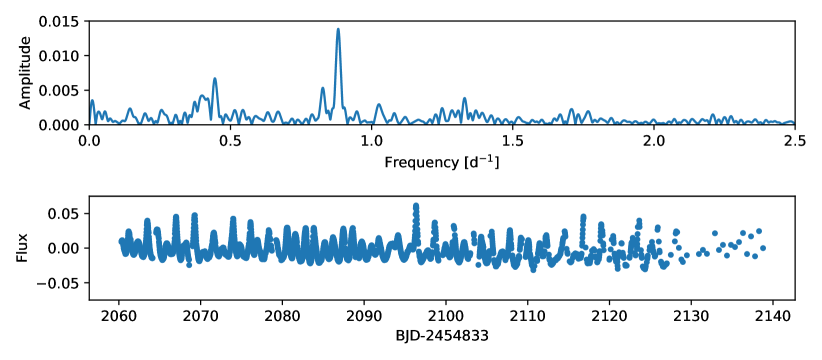
Figure 13: Light curve and frequency spectrum of EPIC 203371239 excluding data obtained during eclipse. A low order polynomial fit by least-squares has been subtracted from the data shown in the lower panel. The flux is measured relative to the mean flux between the eclipses.

3.1.18 EPIC 203543668

The photometric aperture we used to construct the K2 light includes the flux from some nearby stars, but this is not enough to account for the value of $\ell_{3}$ we obtain from the fit to the light curve. The location of these stars in the T_eff – $\rho_{\star}$ plane (Fig. 11) suggests that the primary is a star similar to the Sun and the secondary is a dwarf star with a mass $M\approx 0.7M_{\sun}$. Both stars appear near the zero-age main sequence for solar-metallicity models of stars with these masses for any reasonable choice of the mass ratio, $q$.

3.1.19 EPIC 203610780

The parameters we have derived for this binary system from the analysis of the K2 light curve are quite robust because the eclipses are total. Star 2 is much larger and cooler than star 1 so we can assume $q>1$, but the actual value of $q=1.2$ used to plot the stars in Fig. 11 is quite uncertain. The position of the hotter star below the zero-age main sequence for solar-type stars suggests that this may be a low-metallicity system. This conclusion is not affected by the exact choice of $q$. The complicating factor for this interpretation is the large amount of third light in this system that leads to large uncertainties in the effective temperature estimates.

3.1.20 EPIC 203636784

The rotation signal in the K2 light curve has an amplitude of about 1.5% at the start of the observing sequence that gradually decreases to an amplitude of about 0.5%. The rotation period is consistent with the assumption of pseudo-synchronous rotation. Star 1 has T${}_{\rm eff}\approx 6000$ K while star 2 is much cooler and smaller than star 1 so we assume that this system consists of a solar type star and a K- or M-dwarf companion. The position of the stars in Fig. 11 does not depend strongly on the assumed value of $q$ provided that this value is significantly less than 1. The location of these stars in the T_eff – $\rho_{\star}$ plane (Fig. 11) suggests that the primary is a star near the main-sequence turn-off with a mass $M\approx 1.1M_{\sun}$ and the secondary is a dwarf star with a mass $M\approx 0.7M_{\sun}$.

3.1.21 EPIC 203728604

The K2 light curve of this star between the eclipse shows a well defined periodic signal with a period of 2.306 d and an amplitude of about 400 ppm. The coherence of this signal suggests that this is a pulsation signal rather than rotational modulation due to star spots, perhaps due to $\gamma$ Dor-type pulsations in one of the stars. The location of these stars in the T_eff – $\rho_{\star}$ plane (Fig. 11) suggests that the primary is a star near the main-sequence turn-off with a mass $M\approx 1.5M_{\sun}$ and the secondary is a star similar to the Sun. This conclusion is not affected by the choice of mass ratio for any value $q\ga 0.8$. The mass ratio is almost certainly has a value $q>1$ since star 1 has a much larger radius than star 2. The periodogram of the data between the eclipses for this star is shown in Fig. 14.

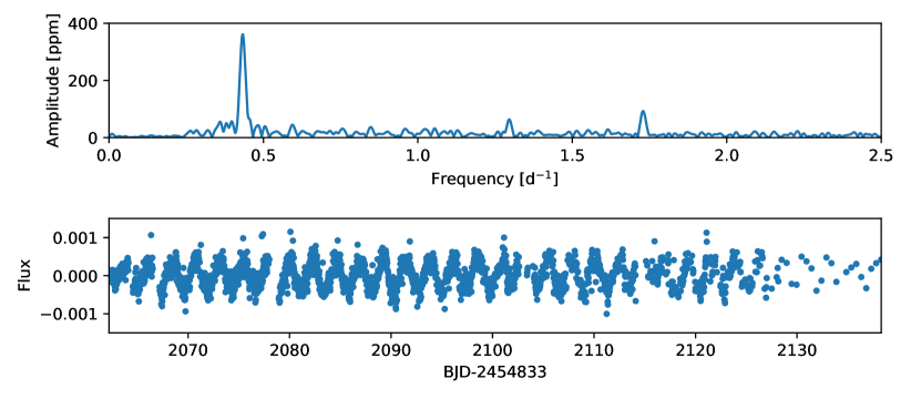
Figure 14: Light curve and frequency spectrum of EPIC 203728604 excluding data obtained during eclipse. A low order polynomial fit by least-squares has been subtracted from the data shown in the lower panel. The flux is measured relative to the mean flux between the eclipses.

3.1.22 EPIC 204407880

The WASP 200-mm data for this star include three nights covering the primary eclipse. To measure the times of mid-eclipse from these data we used a model with the geometric parameters fixed to the values determined from a preliminary fit to the K2 light curve. The three times of mid-eclipse and the surface brightness ratio in the WASP bandpass were free parameters in a fit to the WASP data using emcee to determine the optimum value of these parameters and their standard errors. The times of mid-eclipse derived using this method were BJD${}_{\rm TDB}-2450000=$ 3893.334(2), 4271.385(1), 4649.435(2), where the values in parentheses denote the standard error in the final digit. From a linear fit to these times of mid-eclipse plus the value 2456917.71237(14) from a preliminary fit to the K2 light curve we find an orbital period of $34.36789\pm 0.00002$ d. This period was included as a prior in the analysis of the K2 light curve.

3.1.23 EPIC 204576757

This star is listed as a planetary candidate system with a period of 23.277669 days by Vanderburg et al. (2016), although the estimated radius of the companion ($\sim 3R_{\rm Jup}$) is rather large for a planetary-mass object. Three total eclipses due to the transit of the companion are visible in the K2 light curve but there is no clear secondary eclipse visible in these data. This may be because the companion contributes less than about 0.25% of the flux at optical wavelengths, or the orbital eccentricity may be large enough for there to be no secondary eclipse. Given this ambiguity over the configuration of this binary system we have not attempted any further analysis of the K2 light curve.

3.1.24 EPIC 204748201

Although this is a binary with total eclipses, the secondary eclipse is very shallow so including third light contamination in the analysis results in parameters that have large uncertainties. We decided to fix the third light parameter at $\ell_{3}=0$ for this preliminary characterisation of this system. Star 1 has T${}_{\rm eff}\approx 6100$ K while star 2 is very cool and much smaller than star 1 so we assume that this system consists of a solar type star and a K-dwarf companion. In this case $q$ must be significantly less than 1, so the position of the stars in Fig. 11 does not depend strongly on the assumed value of $q$. With these assumptions, the location of the stars in the T_eff – $\rho_{\star}$ plane (Fig. 11) suggests that they are dwarf stars near the zero-age main sequence with masses $M\approx 1.2M_{\sun}$ and $M\approx 0.5M_{\sun}$.

3.1.25 EPIC 204760247 = HD 142883

This bright B3V star (V=5.84) is listed in SIMBAD as a Cepheid variable star – this is not correct. Hill (1967) found this star to be a variable with a possible period 0.2872 days based on 20 observations in each of the U and B bands but note that ”because of the extremely small amplitude of the variation …this star must be considered a tentative $\beta$ Cephei variable.” Andersen & Nordstrom (1977) noted that this star is a double-lined spectroscopic binary with the secondary component “much fainter”. In a later study (Andersen & Nordstrom 1983) they estimated a mass ratio for this binary of $0.38\pm 0.03$. Levato et al. (1987) report 8 radial velocity measurements from which they claimed the first spectroscopic solution for this star with an orbital period near 10  days, but with a very large eccentricity that is not consistent with the data described below. Koen & Eyer (2002) note that this is a variable star on the basis of the Hipparcos epoch photometry but were not able to classify the type variability. Wraight et al. (2011) used observations from the STEREO mission to correctly identify the variability of this star as being due to eclipses with a period of 9.20 days. This star is a member of the Upper Scorpius OB association (Madsen et al. 2002).

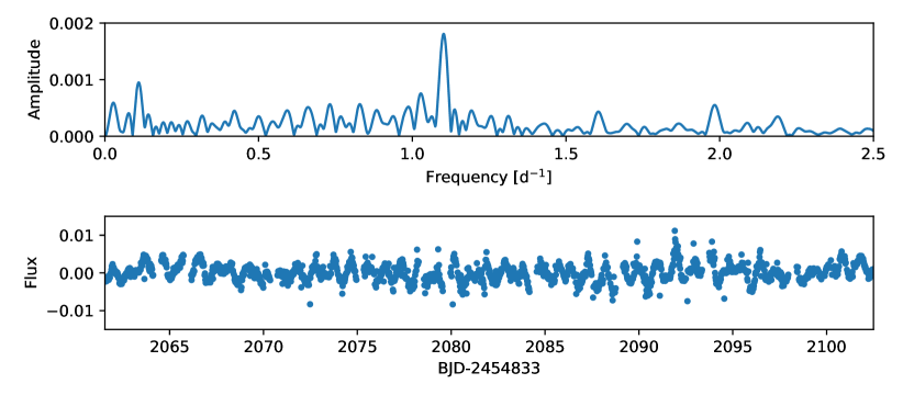
Figure 15: Light curve and frequency spectrum of EPIC 204760247 excluding data obtained during eclipse. A low order polynomial fit by least-squares has been subtracted from the data shown in the lower panel. The flux is measured relative to the mean flux between the eclipses.

We conducted aperture photometry for this star including the extensive charge overspill region provided in the K2 target pixel file. This provided useful photometry for the interval BJD 2456894.5 to 2456935.5. There is a very clear pulsation signal in the data between the eclipses with an period of 0.908 days and an amplitude of 0.18% (Fig. 15). There is also a periodic signal in these data with a period close to the orbital period and an amplitude of 0.1% that may be due to irradiation of the companion star by the B3V primary star. We have not included this effect in our model of the light curve. The surface brightness ratio from a preliminary light curve solution combined with an estimate for the primary star effective temperature $T_{\rm eff}=18,000$ K based on its spectral type implies $T_{\rm eff}\approx 10,000$ K for the secondary star. We used these $T_{\rm eff}$ estimates and the tabulation by Claret & Bloemen (2011) to estimate the quadratic limb darkening coefficients $(a,b)=(0.11,0.24)$ and $(0.21,0.29)$ for the primary and secondary, respectively. We assume standard errors of 0.05 on all these coefficients when imposing them as priors in the light curve analysis.

We downloaded six spectra of this star observed with the FEROS spectrograph from the ESO science archive. We used cross correlation over the wavelength range 400 – 680 nm against a numerical mask from an A0-type template star in iSpec (Blanco-Cuaresma et al. 2014) to measure the radial velocities given in Table 8. The full widths at half minimum (FWHM) of the dips in the cross correlation function (CCF) measured by a simultaneous fit of two Gaussian profiles are 22 km s^-1 and 28 km s^-1 for star 1 and star 2, respectively. A third dip is visible in the CCF with a radial velocity of $-13$ km s^-1 and FWHM of 15 km s^-1 and a strength approximately half that of the peak for star 2. The mismatch between the spectral type of the primary star and the template in this case makes it difficult to interpret the strength of the dip in the CCF for this star – no template is available for spectral type earlier than A0 in the current version of iSpec.

We used emcee to find the best fit Keplerian orbit to these radial velocity measurements assuming a circular orbit ($e=0$). We did not find a satisfactory fit to these data using the values of $T_{0}$ and $P$ taken from the values shown in Table 2. Instead we noted that there is a secondary eclipse visible in the Hipparcos epoch photometry for this star and used this to estimate an orbital period of 9.199724(4) days. With this orbital period imposed as a prior we find that the semi-amplitudes are $K_{1}=62.8\pm 1.7$ km s^-1 and $K_{2}=136.6\pm 1.4$ km s^-1. The masses of the stars are $M_{1}=5.18\pm 0.15$ M_⊙ and $M_{2}=2.38\pm 0.11$ M_⊙ and their radii are $R_{1}=2.50\pm 0.04$ R_⊙ and $R_{2}=1.63\pm 0.04$ R_⊙.

3.1.26 EPIC 204822807

The argument that leads to the conclusion $q\approx 1$ for EPIC 201161715 also applies to this binary system, but in this case it is star 2 that is the cooler and larger star so we assume the value $q=1.1$ to plot the position of the stars in Fig. 11. This system is a bright, totally eclipsing binary system that contains a star on the red giant branch and a star with a mass similar to the Sun near the main-sequence turn-off point, similar to the well-known systems AI Phe (Kirkby-Kent et al. 2016) and TZ For (Valle et al. 2017). This makes this system an attractive target for calibrating stellar models.

3.1.27 EPIC 204870619

This is a long-period binary in which a sub-giant star with a mass $\approx 1.2\,M_{\odot}$ produces total eclipses of a dwarf star with a mass $\approx 0.8\,M_{\odot}$. The position of the stars in the T_eff – $\rho_{\star}$ plane lie near the stellar evolution tracks for these masses for any reasonable choice of $q$ so these masses should be quite accurate. It may be challenging to measure precise radial velocities for the dwarf star in this binary since it only contributes about 5% of the flux at optical wavelengths and the system is quite faint. Nevertheless, this is an attractive target for follow-up observations to test stellar models given that, in principle, the masses and radii for these stars can be determined to an accuracy much better than 1% and there do not appear to be any complications in the analysis due to star spots or pulsations.

3.1.28 EPIC 205020466

We obtained 4 spectra of this star using the High Resolution Spectrograph (HRS) on the Southern African Large Telescope (SALT) (Crause et al. 2014). We used the medium resolution mode to obtain spectra at a resolving power $R=43,000$ on the blue arm of the instrument and $R=40,000$ on the red arm. The exposure time of 577 s on both arms resulted in a signal-to-noise per pixel of approximately 10 on the blue arm and 20 on the red arm. We used spectra reduced automatically using the pipeline developed by Kniazev et al. (2017) for our analysis. We used iSpec (Blanco-Cuaresma et al. 2014) to measure the radial velocities for both stars from Gaussian profile fits to the cross-correlation function (CCF) calculated using a numerical mask based on the solar spectrum. The results of these fits are given in Table 8. We did not attempt any further analysis of the HRS spectra because the signal-to-noise is quite low and the reduced spectra are not corrected for the blaze function of the spectrograph.

We used emcee to find the best fit Keplerian orbit to these radial velocity measurements including Gaussian priors on the parameters $f_{s}$, $f_{c}$, $T_{0}$ and $P$ taken from the values shown in Table 2. We assumed a single value for the standard error on these radial velocity measurements and included this as a free parameter in the analysis by including the appropriate term in the likelihood function. The semi-amplitudes derived from this fit are $K_{1}=60.5\pm 1.3$ km s^-1 and $K_{2}=75.5\pm 1.3$ km s^-1 and the standard error per observation derived is 2.0 km s^-1. The absolute parameters of the stars derived from these values and the data in Tables 2 and 3 are given in Table 7. The masses in this table agree well with the values that can be inferred from the location of the stars in the T_eff – $\rho_{\star}$ plane (Fig. 11) if the errors in T_eff are accounted for.

Table 7: Absolute astrophysical parameters of EPIC 205020466.

	Primary	Secondary
Mass [$M_{\sun}$]	1.05 $\pm$ 0.04	0.84 $\pm$ 0.04
Radius [$R_{\sun}$]	0.89 $\pm$ 0.015	0.86 $\pm$ 0.015
$\log g$ [cm s-2]	4.56 $\pm$ 0.01	4.49 $\pm$ 0.015
Teff [K]	5300 $\pm$ 480	5070 $\pm$ 425
$\log(L/L_{\sun})$	$-0.25\pm 0.16$	$-0.35\pm 0.15$
MV [mag]	5.5 $\pm$ 0.5	5.9 $\pm$ 0.5
Orbital period [d]	8.75903 $\pm$ 0.00003
Mass ratio	0.80 $\pm$ 0.02
Distance [pc]	340 $\pm$ 120

3.1.29 EPIC 205170307

The analysis of this system is complicated by substantial 3rd light contamination ($\ell_{3}\approx 17$%) but the eclipses are total and well-defined so a robust determination of the system parameters is possible. The eclipsing pair are dwarf stars with masses $\approx 0.65\,M_{\odot}$ and $\approx 1.0\,M_{\odot}$ with the more massive star near the main-sequence turn-off point in Fig. 11. The position of the stars in the T_eff – $\rho_{\star}$ plane lie near the stellar evolution tracks for these masses for any reasonable choice of the mass ratio, $q$.

3.1.30 EPIC 205546169

Based on the parameters we have derived, the eclipsing pair in this system are both dwarf stars with masses $\approx 1.2\,M_{\odot}$ with one star near the zero-age main sequence and one near the end of the main sequence. This conclusion does not depend on the assumed mass ratio for any reasonable choice of $q$. We assume $q=1.1$ to plot these stars in Fig. 11 since star 2 is apparently more evolved than star 1. This combination is difficult to reconcile with the very similar effective temperatures for the two stars. The secondary eclipse in this system is very shallow, the eclipses are partial and there may be third-light contamination $\ell_{3}\approx 9$% so the parameters we have derived here may be subject to quite large systematic error. Spectroscopic observations to determine more robust estimates for $\ell_{3}$ and $\ell_{\rm Kp}$ will be very helpful for the analysis of this system.

3.1.31 EPIC 205703649

The photometric aperture we used for this star is contaminated by nearby stars of comparable brightness to the target star. This is accounted for in the photometric fit by including $\ell_{3}$ as a free parameter and accounts for the large value of this parameter. We have assumed that this contaminating flux does not affect the catalogue photometry for the target star and so we set $\ell_{3}=0$ to derive the effective temperature estimates in Table 2.5. With this assumption, both stars appear to be dwarf stars near the MSTO with masses $\approx 1.0\,M_{\odot}$. Star 2 is larger than star 1 so $q>1$ seems a reasonable choice. However, it is very unlikely that both stars would appear near the MSTO if they have different masses, therefore we assume the value $q=1$ for the purposes of plotting these stars in Fig. 11.

3.1.32 EPIC 205919993 = LP 819-72

LP 819-72 was identified as an eclipsing binary using data from the WASP project prior to the start of the K2 mission. The primary eclipse was never observed with WASP because the orbital period is so close to exactly 11 days. As such, it was misclassified as an eclipsing binary with a transiting low mass companion (“EBLM”) with an orbital period of 3.666 days.

We submitted LP 819-72 to the guest observer program on K2 and also obtained 33 spectra of this system with the fibre-echelle spectrograph on the CTIO 1.5-m telescope operated by the SMARTS Consortium. The spectra were typically observed in groups of three with an exposure time of 900 s plus an accompanying arc spectrum for wavelength calibration. We extracted a single order from these echelle spectra using the optimal extraction routines and wavelength calibration routines pamela and molly (Marsh 1989). The spectral order selected covers the wavelength range 660.9 – 647.7 nm and the resolving power of the instrument is $R\approx 37,000$. The signal-to-noise ratio per pixel at the centre of the order is typically ${\rm S/N}\approx 20$. We used iSpec (Blanco-Cuaresma et al. 2014) to measure the radial velocities for both stars in those spectra where the lines from the two stars are clearly resolved. The radial velocities were measured using Gaussian profile fits to the cross-correlation function (CCF) calculated using a numerical mask based on a K5 spectral-type template. The results of these fits are given in Table 8. The individual spectra observed on the night JD 2455477 were of lower signal-to-noise than other spectra so we co-added these spectra for analysis. We also co-added the group of three spectra with the highest S/N in order to look for additional dips in the CCF. No such dips were detected so we estimate that the contribution from any third star in the system does not exceed about 10% at these wavelengths, assuming that any such star is a slowly rotating star with a late-type spectrum.

For simplicity in the analysis below we fixed the third light parameter $\ell_{3}=0$ for our analysis of the K2 light curve. We also imposed a prior on the flux ratio $\ell_{\rm Kp}$ from the ratio of the depths of dips in the CCF. The mean and standard error in the mean in this ratio is $1.28\pm 0.03$ but we use a Gaussian prior on $\ell_{\rm Kp}$ with mean 1.28 and standard deviation 0.05 to allow for some uncertainty in converting the depth of the dip in the CCF to a flux in the Kepler bandpass. This information from the spectroscopy is extremely useful for the analysis of the K2 light curve because without these priors on $\ell_{3}$ and the flux ratio the best-fit solutions tend to imply a flux ratio for the stars that is inconsistent with the radius ratio.

Table 8: Radial velocity measurements.

BJD (UTC)	$V_{r,1}$	$V_{r,2}$
$-2450000$	[km s-1]	[km s-1]
EPIC 202674012, FEROS
6100.635	$-34.2\pm 0.3$	$63.0\pm 0.3$
6102.545	$-21.0\pm 0.3$	$46.9\pm 0.3$
6517.565	$-32.4\pm 0.3$	$61.9\pm 0.3$
7174.732	$-21.6\pm 0.3$	$47.4\pm 0.3$
EPIC 205020466, SALT HRS
7810.574	$-17.1\pm 2.0$	$-103.3\pm 2.0$
7810.574	$-16.2\pm 2.0$	$-102.5\pm 2.0$
7843.498	$-14.6\pm 2.0$	$-97.0\pm 2.0$
7843.498	$-14.2\pm 2.0$	$-95.6\pm 2.0$
7844.484	$-4.5\pm 2.0$	$-104.9\pm 2.0$
7844.484	$-6.8\pm 2.0$	$-104.0\pm 2.0$
7865.654	$-128.4\pm 2.0$	$44.2\pm 2.0$
7865.654	$-128.2\pm 2.0$	$43.9\pm 2.0$
EPIC 205919993, CTIO 1.5-m
5429.806	$50.35\pm 0.39$	$-49.73\pm 0.24$
5429.817	$51.88\pm 0.31$	$-49.10\pm 0.35$
5429.827	$51.52\pm 0.61$	$-49.21\pm 0.26$
5439.699	$55.18\pm 0.62$	$-52.34\pm 0.64$
5439.710	$55.40\pm 0.56$	$-52.70\pm 0.35$
5439.721	$56.07\pm 1.05$	$-52.74\pm 0.49$
5445.628	$-47.66\pm 0.45$	$45.75\pm 0.29$
5445.638	$-48.10\pm 0.34$	$45.72\pm 0.36$
5445.649	$-48.45\pm 0.32$	$47.00\pm 0.44$
5477.643	$-45.65\pm 0.43$	$42.89\pm 0.42$
5490.594	$-42.71\pm 0.44$	$37.00\pm 0.35$
5490.605	$-41.47\pm 0.55$	$36.30\pm 0.37$
5490.615	$-42.89\pm 0.51$	$36.10\pm 0.28$
5510.519	$-49.12\pm 0.37$	$35.58\pm 0.33$
5510.530	$-48.05\pm 0.31$	$35.64\pm 0.30$
5510.540	$-49.56\pm 0.52$	$35.88\pm 0.33$
EPIC 204760247, FEROS
3129.725	$60.6\pm 7.1$	$-135.5\pm 1.6$
3129.735	$59.6\pm 4.9$	$-135.2\pm 1.7$
4298.510	$54.5\pm 2.3$	$-120.8\pm 2.1$
4302.491	$-65.2\pm 2.3$	$133.4\pm 1.7$
6523.599	$56.8\pm 1.5$	$-132.1\pm 1.8$

We used emcee to find the best fit Keplerian orbit to the radial velocity measurement in Table 8 including Gaussian priors on the parameters $f_{s}$, $f_{c}$, $T_{0}$ and $P$ taken from the values shown in Table 2. We find that the semi-amplitudes are $K_{1}=54.1\pm 0.6$ km s^-1 and $K_{2}=49.2\pm 0.6$ km s^-1. The absolute parameters of the stars derived from these values and the data in Tables 2 and 3 are given in Table 9.

Table 9: Absolute astrophysical parameters of LP 819-72 (EPIC 205919993).

	Primary	Secondary
Mass [$M_{\sun}$]	0.59 $\pm$ 0.02	0.65 $\pm$ 0.02
Radius [$R_{\sun}$]	0.60 $\pm$ 0.01	0.58 $\pm$ 0.01
$\log g$ [cm s-2]	4.65 $\pm$ 0.02	4.72 $\pm$ 0.02
Teff [K]	4025 $\pm$ 60	4230 $\pm$ 60
$\log(L/L_{\sun})$	$-1.07\pm 0.03$	$-1.01\pm 0.03$
MV [mag]	8.38 $\pm$ 0.13	8.05 $\pm$ 0.12
Orbital period [d]	11.00009 $\pm$ 0.00006
Mass ratio	1.10 $\pm$ 0.02
Distance [pc]	42.1 $\pm$ 1.1

The distance to this system based on the parallax measurement from Gaia DR1 is $44.9\pm 0.5$ pc. The distance to this system based on the 2MASS K_s-band magnitude transformed to Johnson K-band and the surface brightness – T_eff relation by Kervella et al. (2004) is $42.1\pm 1.0$ pc, which is a fair agreement with the Gaia DR1 estimate, particularly if the suspected systematic error of about 0.22 mas in Gaia DR1 parallax values for stars near the ecliptic is taken into account (Stassun & Torres 2016b). It remains to be seen whether a more accurate estimate of $\ell_{3}$ will lead to better agreement between these distance estimates.

This high proper motion star has a spectral type of K5V (Stephenson 1986). This implies an effective temperature T${}_{\rm eff}\approx 4436$ K, which agrees reasonably well with the average of our estimates of T_eff for the two stars in Table 2.5.

3.1.33 EPIC 205982900 = BW Aqr

A detailed study of this eclipsing binary has been presented by Clausen (1991) based on uvby light curves by Gronbech et al. (1987) and spectroscopic orbits for both components from Imbert (1987). The times of primary and secondary eclipse show apsidal motion with a period of approximately 6000 years (Volkov & Chochol 2014). The projected equatorial rotational velocities of the stars suggest that they both rotate at about half the rate expected assuming pseudo-synchronisation of the rotation with the orbital angular velocity at periastron.

According to linear ephemeris by Kreiner (2004) the 2MASS observations of this star were obtained during primary eclipse so we did not include these data in the analysis to determine the T_eff estimates in Table 2.5. These T_eff estimates are about 250 K cooler than the values from Clausen (1991) based on the dereddened $(b-y)_{0}$ colour indices, which is significant at the 2-$\sigma$ level. This is a consequence of the larger reddening to this system derived by Clausen from Strömgren photometry compared to the value we obtained from broad-band photometry together with the prior on E($\rm B-\rm V$) from reddening maps. The position of these stars in the T_eff – $\rho_{\star}$ plane (Fig. 11) suggest that the higher effective temperature estimate is more reliable given that the masses of these stars are known to be $M\approx 1.4M_{\odot}$.

The K2 light curve of BW Aqr shows an ellipsoidal effect with a semi-amplitude of about 0.1%. To account for this, we set the period of the quasi-periodic kernel used to account for the intrinsic variability of the star in the detrending process to half the orbital period. We then modeled this light curve including the ellipsoidal effect, i.e., we did not divide-out this trend. To account for the ellipsoidal effect and the resulting gravity darkening we used the Roche potential to calculate the shape of the ellipsoids used to model the two stars assuming a mass ratio $q=1$. The gravity darkening exponents were set to $y_{1}=0.267$ and $y_{2}=0.280$ for star 1 and 2, respectively, these values being interpolated from the tabulation by Claret & Bloemen (2011).

The residuals from the our best-fit model light curve show structure at a level of about 500 ppm. The periodogram of these residuals shows peaks at various harmonics of the orbital period. We used light curves derived using the everest algorithm (Luger et al. 2016) to check that these features in the light curve are not a by-product of our data analysis method. We also checked the everest light curves for 3 other stars of similar brightness to BW Aqr and observed during the same K2 campaign and using the same channel of the Kepler instrument. The periodograms of the everest light curves for BW Aqr and one of these comparison stars are shown in Fig. 16. We also analysed the everest light curve for EPIC 201576812 (TYC 272-458-1). For both BW Aqr and TYC 272-458-1 we excluded data obtained during eclipse from the calculation of the periodogram. The rotational modulation of TYC 272-458-1 combined with this masking of the eclipses results in closely separated peaks in the periodogram at harmonics of the orbital frequency up to approximately the 25^th harmonic. In contrast, the periodogram of BW Aqr shows a well defined sequence of single peaks up to the 50^th harmonic of the orbital frequency, at least. A likely interpretation of these frequencies is that they are tidally induced pulsations, similar to those seen in the non-eclipsing binary system KOI-54 (Fuller & Lai 2012; Burkart et al. 2012). The strongest frequencies are at the 2^nd and 3^rd harmonic of the orbital frequency, which agrees well with the expectation for a binary system with an eccentricity e$\approx 0.18$ (Ogilvie 2014, Fig. 3). The detection of tidally induced pulsations in BW Aqr open up the possibility of testing methods to derive stellar parameters using asteroseismology for non-eclipsing binary stars such as KOI-54, and to investigate the role of these pulsations in the circularisation and synchronisation of BW Aqr’s orbit. Such studies will be aided by the availability of K2 data with a temporal sampling of 58.8 s (“SC” data) for this binary system.

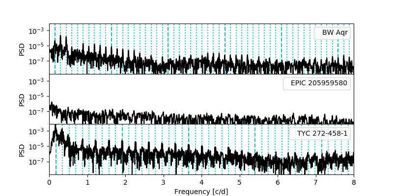
Figure 16: Periodograms of the K2 everest light curves for EPIC 205982900 (BW Aqr) excluding data in eclipse, another star of comparable brightness observed in the same campaign with the same detector module, output and channel (EPIC 205959580), and EPIC 201576812 (TYC 272-458-1) excluding data in eclipse. Vertical lines mark the orbital frequency and its harmonics for the two eclipsing binaries.

Table 10: Absolute astrophysical parameters BW Aqr.

	Primary	Secondary
Mass [$M_{\sun}$]	1.38 $\pm$ 0.02	1.48 $\pm$ 0.02
Radius [$R_{\sun}$]	1.732 $\pm$ 0.008	2.068 $\pm$ 0.009
$\log g$ [cm s-2]	4.100 $\pm$ 0.003	3.977 $\pm$ 0.003
Teff [K]	6450 $\pm$ 100	6350 $\pm$ 100
$\log(L/L_{\sun})$	0.67 $\pm$ 0.03	0.80 $\pm$ 0.03
MV [mag]	3.07 $\pm$ 0.07	2.76 $\pm$ 0.07
Orbital period [d]	6.719683 $\pm$ 0.000004
Mass ratio	0.931 $\pm$ 0.008
Eccentricity	$0.1773\pm 0.0008$
Distance [pc]	411 $\pm$ 21

3.1.34 EPIC 206066862 = BD $-$13$^∘$ 6219

We decided to fix the third light parameter at the value $\ell_{3}=0$ since the eclipses in this light curve are partial and the secondary eclipse is quite shallow. Barros et al. (2016) quote an orbital period P=11.08716751d for this binary, which is in good agreement with our estimate. These stars appear near the evolutionary tracks for masses of $0.8\,M_{\sun}$ and $1.2\,M_{\sun}$ for any reasonable choice of the mass ratio, so we assume $q\approx 0.7$.

3.1.35 EPIC 206066909

The K2 light curve between the eclipses shows variability on timescales of a few days with an amplitude of about 0.1%. We were not able to identify a clear period for this variability and the interpretation of this signal is complicated by a substantial third-light contribution to the light curve in this multiple star system. The position of the stars in the T_eff – $\rho_{\star}$ plane lie near the stellar evolution tracks for masses $0.7\,M_{\sun}$ and $1.3\,M_{\sun}$ for any reasonable choice of the mass ratio so we assume $q\approx 0.5$.

3.1.36 EPIC 206075677

There are two partial secondary eclipses visible in the detrended K2 light curve with depths of 0.4% and 1.5% following division by the trends in the light curve due to star spot modulation. These trends show an amplitude of 1.5% and at least three well defined peaks in the periodogram at the periods listed in Table 1. Given the complexity of this system and the lack of unambiguous information in the light curve, we decided not to attempt a model fit to this light curve.

3.1.37 EPIC 206084435

There is only one primary eclipse visible in the K2 light curve for this very long-period binary ($P\approx 48$ d) so the period is determined from the two shallow secondary eclipses. The primary star is a main-sequence star with a mass $M\approx 1.1M_{\odot}$ and the companion is a dwarf star with a mass $M\approx 0.65M_{\odot}$. The position of the stars in the T_eff – $\rho_{\star}$ plane lie near the stellar evolution tracks for these masses for any reasonable choice of the mass ratio, $q$.

3.1.38 EPIC 206109641

The K2 light curve of this star shows two eclipses with unequal depths separated by 7.68 days. Only one eclipse of each depth in visible within the 69.16 day span of the K2 observations. From the K2 data alone it is only possible to establish a lower limit to the orbital period of 41.77 days. Data from the WASP archive includes one night of 200-mm data covering the minimum of the secondary eclipse at HJD 2455141.285, another night of 200-mm data showing the start of the ingress to primary eclipse at HJD 2454632.6 and one night of 85-mm data covering the egress to the secondary eclipse at HJD 2456144.43. The only period consistent with these observations plus the lack of visible eclipses on other nights for which we have WASP data is $P\approx 62.6$ d.

We included the WASP photometry from the nights listed above plus data from a few additional nights to set the out-of-eclipse level in our analysis of the K2 light curve. The additional parameters required in the fit were the surface brightness ratio for the 200-mm WASP data, $S_{\rm 200}$, the surface brightness ratio for the 85-mm WASP data, $S_{\rm 85}$, the zero-points of the 85-mm and 200-mm data, and the standard deviation of the residuals for the 85-mm and 200-mm data sets, $\sigma_{\rm 200}$ and $\sigma_{\rm 85}$, respectively. Given the quality of the WASP data we decided to use the same limb darkening coefficients and values for third light for these data as for the K2 data rather than adding even more free parameters to the fit. The best-fit model light curves to the K2 and WASP data are shown in Fig. 17. The best-fit values of the additional parameters were found to be $S_{\rm 200}=0.57\pm 0.01$, $S_{\rm 85}=0.42\pm 0.02$, $\sigma_{\rm 200}=0.016$ and $\sigma_{\rm 85}=0.077$. Both stars lie near the position of the Sun in the T_eff – $\rho_{\star}$ diagram for any reasonable choice of mass ratio but the relative position of the stars is inconsistent with star 1 being larger and therefore more evolved unless $q\approx 0.9$.

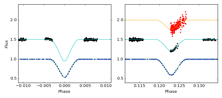
Figure 17: K2 and WASP light curves of EPIC 206109641 around primary and secondary eclipse. The WASP 200-mm and 85-mm data are shown offset vertically by 0.5 and 1 units, respectively. Solid lines show our best-fit light curve model.

3.1.39 EPIC 206212261

The occultation of a dwarf star with a mass $M\approx 0.6M_{\odot}$ by a 1.0-$M_{\odot}$ star near the MSTO results in well-defined total eclipses in the K2 light curve of this system, so the parameters are determined to good precision despite the extreme flux ratio in this binary $\ell_{\rm Kp}\approx 1.7$%. This extreme flux ratio may make it challenging to obtain spectroscopic observations to determine the masses of these stars. Star 1 has T${}_{\rm eff}\approx 5400$ K while star 2 is cooler and much smaller than star 1 so we assume that this system consists of a solar type star and a K-dwarf companion. In this case $q$ must be significantly less than 1, so the position of the stars in Fig. 11 does not depend strongly on the assumed value of $q$.

3.1.40 EPIC 206241558

The K2 light curve of this star shows two eclipses with unequal depths separated by 12.32 days. Only one eclipse of each depth in visible within the 69.16 day span of the K2 observations. From the K2 data alone it is only possible to establish a lower limit to the orbital period of 53.1 days. Data from the WASP archive includes one night of 200-mm data covering the minimum of the primary eclipse at HJD 2455012.63 and another night of 200-mm data covering the egress to the secondary eclipse at HJD 2454685.4. The only period consistent with these observations plus the lack of visible eclipses on other nights for which we have WASP data is $P\approx 56.6$ d.

We included the WASP photometry from the nights listed above plus data from one additional night to set the out-of-eclipse level in our analysis of the K2 light curve. Given the quality of the WASP data we decided to use the same limb darkening coefficients and values for third light for these data as for the K2 data.

We made several attempts to find a combination of starting parameters for the emcee analysis that lead to best-fit solutions with both $k<1$ and $S_{\rm Kp}<1$ or vice versa, but always found that the Markov chains converged on solutions with $k<1$ and $S_{\rm Kp}>1$ or vice versa, depending on the initial parameters and whether or not we fixed $\ell_{3}=0$. We did not find any combination of parameters for which the two stars appear near the same isochrone in the effective temperature – mean stellar density plane so our estimate for the mass ratio $q\approx 1.0$ is very uncertain in this case. One possibility is that this star is the result of a merger between two stars in a triple system induced by Kozai-Lidov cycles in a triple star system (Sandquist et al. 2018). The best-fit model light curves to the K2 and WASP data are shown in Fig. 18. The surface brightness ratio in the 200-mm WASP data we found to be $S_{\rm 200}=1.5\pm 0.1$ and the standard deviation for the residuals is $\sigma_{\rm 200}=0.023$.

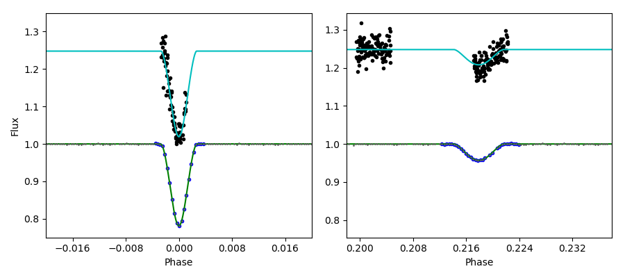
Figure 18: K2 and WASP light curves of EPIC 206241558 around primary and secondary eclipse. Small gray points in the K2 light curve were not included in the fit. The WASP 200-mm data are shown offset vertically by 0.5 units. Solid lines show our best-fit light curve model.

3.1.41 EPIC 206253908

The K2 light curve of this star shows only one eclipse, from which it is possible to establish a lower limit to the orbital period of 62.7 days. Eclipses are also seen in the WASP archive photometry at HJD 2454758.41 and 2455085.61. We estimate the period of this binary to be 65.45 d. As there is no secondary eclipse visible in the K2 or WASP data we did not attempt any further analysis of this star.

3.1.42 EPIC 206288770

The occultation of a dwarf star with a mass $M\approx 0.6\,M_{\odot}$ by a 1.2-$M_{\odot}$ main-sequence star results in well-defined total eclipses in the K2 light curve of this system, so the parameters are determined to good precision despite the extreme flux ratio in this binary $\ell_{\rm Kp}\approx 1.4$%. These mass estimates are quite robust because the position of the stars in the T_eff – $\rho_{\star}$ plane lie near the stellar evolution tracks for these masses for any reasonable choice of $q$. The extreme flux ratio in this binary may make it challenging to obtain spectroscopic observations to determine the masses of these stars.

3.1.43 EPIC 206433263

This eclipsing binary is a favourable target for detailed study of a star similar to the Sun. The eclipses of the star with a mass $M\approx 1.0\,M_{\odot}$ are total and the companion with a mass $M\approx 1.2\,M_{\odot}$ is near the MSTO. These mass estimates are quite robust because the position of the stars in Fig. 11 lie near the stellar evolution tracks for these masses for any reasonable choice of $q$. The optical flux ratio is favourable for spectroscopic follow-up to determine accurate masses for both stars and the star is moderately bright. The mass of the star near the MSTO will put a tight constraint on the age of the system and there do not appear to be any complications due to star spots or third light contamination.

4 Summary and conclusions

We have used light curves from Kepler K2 to identify 42 long-period eclipsing binary systems ($P\ga 5.5$ d) with narrow eclipses and little or no ellipsoidal effect, i.e., well-detached binaries with very weak tidal interaction between the stars. This includes systems with periods $P\ga 60$ d for which the orbital period cannot be established from the K2 data alone (EPIC 206109641, EPIC 206241558 and EPIC 206253908). In these cases we have used data from the WASP project data archive to establish the orbital period of the binary system.

For 40 targets we have determined the geometry of the binary system (fractional radii, inclination, eccentricity, etc.) from the analysis of the Kepler K2 light curve using the ellc eclipsing binary star model. For 38 of these systems we also estimate the effective temperature of the stars from an analysis of the observed apparent magnitudes and other data for the system. For these 38 systems we are able to estimate the mass and evolutionary state of the stars by comparing their mean stellar densities and effective temperatures to stellar models. They typically contain main-sequence or sub-giant stars with masses from 0.6 $M_{\odot}$ to 1.4 $M_{\odot}$, with sub-giant and giant companions being more common among the longer-period systems.

We have used new radial velocity measurements to make preliminary estimates of the mass, radius and luminosity of the stars in 3 systems (EPIC 202674012, EPIC 205020466, EPIC 205919993). We have also re-calculated these absolute parameters for two systems with spectroscopic orbits that have been previously studied using light curves from ground-based instruments (EPIC 201576812 = FM Leo and EPIC 205982900 = BW Aqr). We have also estimated the masses and radii of the eclipsing stars in the early-type triple system EPIC 204760247 = HD 142883.

We confirm the presence of variability between the eclipses in HD 142883 due to $\beta$ Cephei-type pulsations. Variability in the light curve between the eclipses due to $\gamma$ Doradus-type pulsations is seen in EPIC 203371239 and perhaps also EPIC 203728604. In BW Aqr we find variability due to pulsations which we suspect are induced by dissipation of tidal forces in this eccentric binary. Variability due to magnetic activity is seen in several systems and has been used to measure the rotation periods of one or both stars in 13 cases.

Kepler K2 provides almost continuous observations for each campaign field for up to 80 days. This makes it possible to identify and characterise long-period eclipsing binary stars that are very hard to find and study using ground-based observations. The high quality of the photometry also makes it possible to identify features in the light curve such as low-amplitude rotational modulation due to star spots and pulsations that are also very hard to observe from the ground. The high quality of the photometry also enables the geometry of these eclipsing binaries to be measured to very high precision, particularly for those that show total eclipses. Additional work is needed to establish the accuracy of the parameters for eclipsing binary stars that can be derived using Kepler K2 photometry.

The majority of the eclipsing binary systems we have identified in the Kepler K2 data with long orbital periods ($P\goa 10$ d) contain dwarf or sub-giant stars. The high quality of the K2 photometry makes it possible to identify binaries where one star has a much lower mass than the other. These are useful systems for testing stellar evolution models because free-parameters in the models such as the mixing length parameter will affect the two stars in the binary in different ways. It can be challenging to obtain accurate mass estimates for the stars in such binaries because they often have extreme luminosity ratios as optical/infra-red wavelengths, but there are now several high-resolution spectrographs available on large telescopes that should make detailed characterisation for some of these systems feasible.