Anomalous Hall effect in dense QCD matter

Abstract

In this letter, we investigate the anomalous Hall effect in dense QCD matter. When the dual chiral density wave which is the spatially modulated chiral condensate appears in the medium, it gives rise to two Weyl points to the single-particle energy-spectrum and then the anomalous Hall conductivity becomes nonzero. Then, dense QCD matter is analogous to the Weyl semimetal. The direct calculation of the Hall conductivity by way of Kubo’s linear response theory gives the term proportional to the distance between the Weyl points. Unlike the Weyl semimetal, there appears the additional contribution induced by axial anomaly.

Introduction:

It has been recently conceived that quantum chromodynamics (QCD) and condensed matter physics share several important properties in phase transition phenomena such as the spontaneous symmetry breaking, Higgs mechanism and topological structure of matters. In this letter, we clarify deep relations between QCD and Weyl semimetal from the topological viewpoint.

Understanding of the QCD phase structure at finite temperature ($T$) and baryon chemical potential ($\mu$) is one of the important subjects in nuclear, hadron, and elementary particle physics. It should be also interesting in the light of condensed matter physics. One promising approach to access the QCD phase diagram is the lattice QCD simulation which is a powerful gauge-invariant approach to investigate non-perturbative properties. The lattice QCD simulation, however, has the well-known sign problem at finite $\mu$. Thus, one can only reach the region, $\mu/T<1$, even if we utilize several methods to circumvent the sign problem; see Ref. de Forcrand (2009) as an example. Therefore, several effective models haven been used to investigate the QCD phase structure, qualitatively.

Recently, the chiral condensate with the spatial modulation attracts much attention in QCD. The inhomogeneous chiral phase (iCP) is characterized by the generalized order parameter,

$$M\equiv\langle{\bar{\psi}}\psi\rangle+i\langle{\bar{\psi}}i\gamma_{5}\tau_{3}\psi\rangle=\Delta({\bf r})e^{i\theta({\bf r})}$$ (1)

for $SU(2)_{L}\times SU(2)_{R}$, where $\langle{\bar{\psi}}\psi\rangle$ and $\langle{\bar{\psi}}i\gamma_{5}\tau_{3}\psi\rangle$ represent the scalar and pseudo-scalar quark condensates with the quark field $\psi$, respectively. The amplitude or phase of the quark condensates can be spatially modulating. There have been studied various iCP structures by solving the self-consistent equations within the effective model of QCD such as the Nambu-Jona-Lasinio (NJL) model Buballa and Carignano (2015). The typical forms of inhomogeneous chiral condensates with one-dimensional modulations are the dual chiral density wave (DCDW) Nakano and Tatsumi (2005) and the real kink crystal (RKC) Basar et al. (2009); *Nickel:2009wj; $M(z)=\Delta e^{iqz}$ for DCDW, and $M(z)=\frac{2\Delta\sqrt{\nu}}{1+\sqrt{\nu}}\mathrm{sn}\Bigl{(}\frac{2\Delta z}{1+\sqrt{\nu}},\nu\Bigr{)}$ for RKC, where $\Delta\in\mathbb{R}$ is a constant amplitude, $q\in\mathbb{R}$ denotes a wave-number of the one-dimensional modulation in the $z$ direction and $\mathrm{sn}(x,\nu)$ denotes the Jacobi elliptic function with modulus $\nu\in[0,1]$.

In this letter, we focus on the DCDW phase to see an interesting topological aspect. In the recent paper Ferrer and de la Incera have pointed out that anomalous transport should be present in the DCDW phase under the external magnetic field, by modifying the Maxwell equations, which they called axion electrodynamics Ferrer and de la Incera (2015); *Ferrer:2016toh: They found that the system induces the anomalous dissipationless Hall current and the anomalous electric charge density. Since its various consequences should be important phenomenologically, it is indispensable to carry out further investigations.

The quark eigenenergy can be then given by diagonalizing the Hamiltonian within the mean-field approximation; the spectrum is symmetric with respect to zero and the positive-energy solutions render

$$E_{s}({\bf p})=\sqrt{E_{0}^{2}+\frac{|{\bf q}|^{2}}{4}+s\sqrt{({\bf q}\cdot{\bf p})^{2}+m^{2}|{\bf q}|^{2}}},$$ (2)

using the NJL model in the chiral limit, where $s=\pm$, $m=-2G\Delta$ and $E_{0}=\sqrt{p^{2}+m^{2}}$ here $G$ is the coupling constant of the four-quark interaction; for example, see Ref.Nakano and Tatsumi (2005). In following, we set $\mathbf{q}=(0,0,q)$.

The phase transition triggers off the instability of the Fermi surface similar to nesting, so that the value of $q$ is much bigger than $m$, $q/2\gg m$ Tatsumi and Nakano (2004); Nakano and Tatsumi (2005). Figure 1 shows a schematic view of the quark energy spectrum for the cases with $m<q/2$ ((I)), $m>q/2$ ((II)) and $m=q=0$ ((III)), respectively.

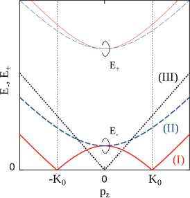
Figure 1: The single-particle spectrum as a function of $p_{z}$ with $p_{\perp}=0$. The cases (I), (II) and (III) represent the situation with $m<q/2$, $m>q/2$ and $m=q=0$, respectively. The thick and thin lines denote $E_{-}$ and $E_{+}$, respectively.

The cases (I) and (II) are analogous to the Weyl semimetal and the spin-splitting insulator, respectively. There appear two nodes called the Weyl points, $K_{0}=\sqrt{(q/2)^{2}-m^{2}}$ and $-K_{0}$, in the case (I); for example see Ref. Murakami (2007). The Dirac Hamiltonian can be well approximated by the $2\times 2$ Weyl Hamiltonian in the vicinity of each Weyl point. The monopole-anti-monopole pair appears at the Weyl points and it gives rise to topological effects. The valence band is the Dirac sea and the conduction band corresponds to the Fermi sea in the DCDW state. Since the chemical potential is nonzero, we can regard the DCDW state as a Weyl metal.

The Weyl semimetal is a topological material in three dimensions and recently attracts much attention experimentally and theoretically in condensed matter physics; for example, see Ref. Yan and Felser (2017); Armitage et al. (2018); Sekine and Nomura (2016). It is known that we can expect anomalous Hall effect (AHE) in the Weyl semimetal. Applying the electric field $E$ along the $y$ axis, the electric current density along the $x$ axis $\langle j_{x}\rangle_{E}$ can be measured: the anomalous Hall conductivity is then calculated as

$$\sigma_{xy}\equiv\frac{\langle j_{x}\rangle_{E}}{E} =\frac{e^{2}}{(2\pi)^{2}}d_{\rm WP},~{}~{}~{}\sigma_{ii}=\sigma_{xz}=\sigma_{zx}=0,$$ (3)

where $d_{\rm WP}=2K_{0}$ is the distance between the Weyl points, $e$ denotes the elementary charge and $i=x,y,z$ Wan et al. (2011); *yang2011quantum; Liu et al. (2017). AHE can be expected, e.g., by doping the magnetic impurities in the Weyl semimetal. Correspondingly, DCDW bears a ferromagnetic property Yoshiike et al. (2015); when we evaluate magnetization in response to the external magnetic field $B$, we can see it survives nonzero in the limit $B\rightarrow 0$, and the finite residual is given by the odd function of the wave number $q$. Thus we may expect a similar phenomenon in the DCDW phase.

In this letter we evaluate the anomalous Hall conductivity by using the Thouless-Kohmoto-Nightingale-den Nijs (TKNN) formula Thouless et al. (1982). We start from the Dirac Hamiltonian with DCDW and calculate the anomalous Hall conductivity by way of Kubo’s linear-response theory. We shall see that the anomalous Hall current is actually induced in the DCDW phase because of the existence of Weyl points. We also discuss its relation to axial anomaly in medium and its implications of the anomalous transport properties of dense QCD matter.

Anomalous Hall conductivity:

We start from the two-flavor Dirac Hamiltonian with the DCDW;

$${\cal H} =\left(\begin{array}[]{ccc}\sigma\cdot(\mathbf{p}-\mathbf{q}\tau_{3}/2)&m\\ m&-\sigma\cdot(\mathbf{p}+\mathbf{q}\tau_{3}/2)\end{array}\right),$$ (6)

where $\sigma$ and $\tau$ represent Pauli matrices for the spin and flavor spaces, respectively. The positive single-particle spectrum is then given by

$$E_{s}({\bf p}) =\sqrt{p_{\perp}^{2}+\Bigl{(}\sqrt{m^{2}+p_{z}^{2}}+s\frac{q}{2}\Bigr{)}^{2}},$$ (7)

and the negative spectrum does $-E_{s}(\mathbf{p})$. When $m$ and $q$ are non-zero, the spectrum split into two branches and then we have two Weyl points. The corresponding eigenspinors are

$$u_{s}({\bf p}) =N_{s}\left(\begin{array}[]{ccc}\psi^{(s)}_{L}({\bf p})\\ \psi^{(s)}_{R}({\bf p})\end{array}\right),$$ (10)

$$v_{s}({\bf p}) =u_{s}({\bf p})\Bigl{|}_{E_{s}({\bf p})\to-E_{s}({\bf p})}$$ (11)

where each component is expressed as

$$\psi_{R}^{(s)}({\bf p}) =\left(\begin{array}[]{ccc}\cfrac{{\tilde{E}_{s}}({\bf p})}{p_{\perp}^{2}}p_{-}\\ -1\end{array}\right),$$ (14)

$$\psi_{L}^{(s)}({\bf p}) =-\frac{m}{{\tilde{\epsilon}_{0}}(p_{z})}\sigma_{3}\psi_{R}^{(s)}({\bf p}),$$ (15)

with $p_{\pm}=p_{x}\pm ip_{y}$ and $\mathbf{p}_{\perp}=p_{x}^{2}+p_{y}^{2}$. The normalization factor then becomes

$$N_{s}^{2} =\frac{{\bf p}_{\perp}^{2}{\tilde{\epsilon}_{0}}(p_{z})}{4s\epsilon_{0}(p_{z})E_{s}({\bf p}){\tilde{E}_{s}}({\bf p})},$$ (16)

where

$${\tilde{E}_{s}}({\bf p}) =E_{s}({\bf p})-s\epsilon_{0}(p_{z})-\frac{q}{2},$$

$$\epsilon_{0}(p_{z}) =\sqrt{p_{z}^{2}+m^{2}},~{}~{}~{}~{}{\tilde{\epsilon}_{0}}(p_{z})=p_{z}+s\epsilon_{0}(p_{z}).$$ (17)

Then, the Berry connection for the positive energy states is defined via the momentum derivative as

$$a^{(s)}_{i}({\bf p}) =-i\Bigl{\langle}u_{s}({\bf p})\hskip 1.42262pt\Bigl{|}\frac{\partial}{\partial p_{i}}\Bigl{|}\hskip 1.42262ptu_{s}({\bf p})\Bigl{\rangle},$$ (18)

and its curvature becomes

$$b_{s,xy}({\bf p}) =\frac{\partial a_{y}^{(s)}({\bf p})}{\partial p_{x}}-\frac{\partial a_{x}^{(s)}({\bf p})}{\partial p_{y}}$$

$$=-i\Bigl{[}\frac{\partial u_{s}^{\dagger}({\bf p})}{\partial p_{x}}\frac{\partial u_{s}({\bf p})}{\partial p_{y}}-\frac{\partial u_{s}^{\dagger}({\bf p})}{\partial p_{y}}\frac{\partial u_{s}({\bf p})}{\partial p_{x}}\Bigr{]}.$$ (19)

The anomalous Hall conductivity in the $3+1$ dimensional system is then expressed as

$$\sigma_{xy} =e^{2}\sum_{s}\int\frac{dp_{z}}{2\pi}\int\frac{d^{2}{\bf p}_{\perp}}{(2\pi)^{2}}\Bigl{[}b_{s,xy}({\bf p})f(E_{s}({\bf p}))\Bigr{]},$$ (20)

where $f(E)$ is the Fermi-Dirac distribution function and $e^{2}$ comes from the cancellation due to different directions of the wave vector for $u$ and $d$ quarks, $N_{\mathrm{c}}(e_{\mathrm{u}}^{2}-e_{\mathrm{d}}^{2})$ with $(e_{\mathrm{u}},e_{\mathrm{d}})=(2e/3,-e/3)$ and $N_{\mathrm{c}}=3$. After few straightforward calculations, the Berry curvature is finally expressed as

$$b_{s,xy}({\bf p}) =-\frac{1}{2E_{s}^{3}}\Bigl{(}s\epsilon_{0}+\frac{q}{2}\Bigr{)}.$$ (21)

When we evaluate contributions from the negative energy-spectrum, $E_{s}$ should be replaced with $-E_{s}$ in Eqs. (20) and (21). It should be noted that $b_{s,xz}$ and $b_{s,yz}$ become the odd function for $p_{x}$, $p_{y}$ or $p_{z}$, respectively. Therefore, we have $\sigma_{xz}=\sigma_{yz}=0$.

Since $\mu$ is finite in the DCDW phase, the Hall conductivity $\sigma_{xy}$ consists of two parts, $\sigma_{xy}=\sigma_{xy}^{\rm Dirac}+\sigma_{xy}^{\rm Fermi}$, where $\sigma_{xy}^{\rm Dirac}$ and $\sigma_{xy}^{\rm Fermi}$ are the contributions from the Dirac sea and the Fermi sea, respectively.

First, we consider the contribution of the Dirac sea at $T=0$ because inclusion of the Fermi sea is straightforward. The anomalous Hall conductivity can be expressed as

$$\sigma_{xy}^{\rm Dirac} =e^{2}\sum_{s}\int\frac{dp_{z}}{2\pi}\int\frac{d^{2}{\bf p}_{\perp}}{(2\pi)^{2}}\Bigl{[}\frac{1}{2E_{s}^{3}}\Bigl{(}s\epsilon_{0}+\frac{q}{2}\Bigr{)}\Bigr{]}$$

$$=\frac{e^{2}}{(2\pi)^{2}}\lim_{\Lambda\to\infty}\sum_{s}\int_{0}^{\Lambda_{z}}dp_{z}\left\{\mathrm{sgn}\Bigl{(}s\sqrt{m^{2}+p_{z}^{2}}+q/2\Bigr{)}-\frac{s\sqrt{m^{2}+p_{z}^{2}}+q/2}{\sqrt{\Lambda_{\perp}^{2}+(\sqrt{m^{2}+p_{z}^{2}}+sq/2)^{2}}}\right\},$$ (22)

where $\mathrm{sgn}(\cdot)$ means the sign function and $\Lambda_{\perp}$ and $\Lambda_{z}$ are related with $\Lambda$; $\Lambda_{\perp}=\Lambda_{z}=\Lambda$ for the three-dimensional momentum cutoff scheme and $\Lambda_{\perp}=\sqrt{\Lambda^{2}-(\epsilon_{0}+sq/2)^{2}}$ and $\Lambda_{z}=\sqrt{(\Lambda-sq/2)^{2}-m^{2}}$ for the energy cutoff scheme. Unfortunately, the anomalous Hall conductivity depends on the cutoff scheme;

$$\sigma_{xy}^{\mathrm{Dirac}} =e^{2}\times\begin{dcases}C,&m>\frac{|q|}{2}\\ C+\mathrm{sgn}(q)\frac{d_{\rm WP}}{(2\pi)^{2}},&m<\frac{|q|}{2}\\ \end{dcases}$$ (23)

where $C$ denotes the cutoff dependent term. In the three-dimensional momentum cutoff scheme, $C=-q/(6\pi^{2})$. In contrast, $C$ becomes $-q/(2\pi)^{2}$ in the energy cutoff scheme. Such cutoff dependence is well known in the study of the Weyl semimetal Grushin (2012); Goswami and Tewari (2013); we must impose a physical condition to fix the cutoff dependence. In the physical situation $C$ should be vanished because the anomalous Hall conductivity should be zero for the insulator ($m>|q|/2$) and gives Eq. (3) for the Weyl semimetal ($m<|q|/2$) . On the other hand, another criterion is needed to remove ambiguity for $C$, when DCDW appears in QCD; the condition $m<|q|/2$ is always satisfied in the DCDW phase and the massless limit ($m\rightarrow 0$) implies the disappearance of DCDW. If $C$ is vanished, AHE remains in the normal quark phase and then the nonzero anomalous Hall conductivity is unphysical. Thus $\sigma_{xy}^{\rm Dirac}\rightarrow 0$ as $m\rightarrow 0$. This is achieved in the gauge invariant regularizations such as the proper-time method or the heat-kernel method Tatsumi et al. (2015). The energy cutoff scheme can give the same answer in the present case,

$$\sigma^{\mathrm{Dirac}}_{xy} =e^{2}\times\begin{dcases}-\frac{q}{(2\pi)^{2}},&m>\frac{|q|}{2}\\ -\frac{q}{(2\pi)^{2}}+\mathrm{sgn}(q)\frac{d_{\rm WP}}{(2\pi)^{2}},&m<\frac{|q|}{2}.\\ \end{dcases}$$ (24)

This is our main result in this letter. Note that only the lower case is realized in the DCDW phase to give the anomalous Hall current,

$${\bf j}_{\rm AHE} =\frac{e^{2}}{(2\pi)^{2}}\left(1-\frac{d_{\rm WP}}{|q|}\right){\bf q}\times{\bf E}.$$ (25)

We shall see that the first term stems from the effect of axial anomaly. In the $m\to 0$ limit, AHE disappears which means that axial anomaly exactly eliminates the anomalous Hall current in QCD.

Next, we take into account the Fermi-sea contributions. The Fermi-sea contributions for the cases (a) $\mu<q/2-m$, (b) $q/2-m<\mu<q/2+m$ and (c) $q/2+m<\mu$ become

$$\sigma_{xy}^{\rm Fermi} =\frac{e^{2}}{(2\pi)^{2}}\Bigl{[}\frac{1}{2\mu}\Bigl{(}\mu+\frac{q}{2}\Bigr{)}^{2}\sin\theta_{+}-\frac{1}{2\mu}\Bigl{(}\mu-\frac{q}{2}\Bigr{)}^{2}\sin\theta_{-}-\frac{m^{2}}{4\mu}\ln\frac{(1+\sin\theta_{+})(1-\sin\theta_{-})}{(1-\sin\theta_{+})(1+\sin\theta_{-})}-d_{\mathrm{WP}}\Bigr{]},$$ (26)

where $\sin\theta_{+}=\sqrt{1-m^{2}/(\mu+q/2)^{2}}$, and $\sin\theta_{-}=\sqrt{1-m^{2}/(\mu-q/2)^{2}}$ for (a) or (c) and $\theta_{-}=0$ for (b). For the Fermi-sea contribution, we do not need to fix the cutoff scheme because the step function acts as the natural cutoff. Figure 2 shows the $\mu$-dependence of $\sigma_{xy}^{\mathrm{Fermi}}$ with fixed $m$ and $q$. It correctly approaches to zero with $\mu\to 0$. In the realistic situation, $m$ and $q$ changes as functions of $\mu$ , and thus we must carefully extract the effect of $\sigma_{xy}^{\mathrm{Fermi}}$.

Figure 2: The $\mu$-dependence of $\sigma_{xy}^{\mathrm{Fermi}}$ with fixed $m$ and $q$.

By taking $m\to 0$ limit, we have $\sigma^{\mathrm{Fermi}}\to 0$ and thus this expression is suitable from the viewpoint of the normal quark matter behavior.

Discussion:

One may wonder whether our result can be derived from considerations of axial anomaly Zyuzin and Burkov (2012). Actually, using Fujikawa’s method, Ferrer and de la Incera have discussed AHE and axion electrodynamics in the DCDW phase in the presence of the background electromagnetic field Ferrer and de la Incera (2015); *Ferrer:2016toh. Since the Dirac Hamiltonian (4) can be obtained by the local chiral transformation on the quark field, $\psi\rightarrow{\rm exp}(-i\tau_{3}\gamma_{5}\theta/2)\psi$, with $\theta={\bf q}\cdot{\bf r}$ from the original one, the anomaly term should appear in the action in the presence of the electromagnetic field, $S_{\mathrm{anom}}=-(e^{2}/16\pi^{2})\int d^{4}x\theta~{}F_{\mu\nu}{\tilde{F}}^{\mu\nu}$. The variation of $S_{\mathrm{anom}}$ with respect to $A_{i}$ gives the anomalous Hall current, $j_{\mathrm{anom}}^{i}=-\delta S_{\mathrm{a}nom}/\delta A_{i}$;

$$j^{i}_{\mathrm{anom}}=\frac{e^{2}}{4\pi^{2}}\nabla\theta\times{\mathbf{E}}=\frac{e^{2}}{4\pi^{2}}{\mathbf{q}}\times{\mathbf{E}},$$ (27)

from which the anomalous Hall conductivity reads as $\sigma_{xy}=-e^{2}/(4\pi^{2})q$. Note that this expression is incorrect in comparison with Eq. (24). Instead, we can see that the first term in Eq. (24) comes from axial anomaly.

We can see the similar situation in the evaluation of anomalous quark number, which is brought about by spectral asymmetry of the quark fields. It has been shown that spectral asymmetry does not necessarily gives the same result as the one given by axial anomaly Tatsumi et al. (2015): it coincides with each other only in the case, $q/2\ll m$ which is corresponding to the situation that the Weyl points disappear. This means that we can not reach the total amount of the anomalous quark number by only using Fujikawa’s method. To evaluate the anomalous transport coefficients correctly, we must use Kubo’s linear response theory.

Summary:

In this letter, we have considered the anomalous Hall effect (AHE) in dense QCD matter. At finite density, we can expect that the spatial inhomogeneity appears in the chiral condensate as the dual chiral density wave (DCDW) and the DCDW can lead topologically nontrivial properties to QCD such as AHE.

Starting from the Dirac Hamiltonian with DCDW, we can evaluate the Berry connection and its curvature from the one-particle spectrum and corresponding eigen-functions. Then, the anomalous Hall conductivity can be obtained by way of the TKNN formula based on Kubo’s linear response theory. It is found that dense QCD matter can exhibit AHE when DCDW appears. Depending on the strength of the amplitude ($m$) and the phase ($q$) of DCDW, the anomalous Hall conductivity shows the different functional form but it is always nonzero with $q\neq 0$ except for the $m\to 0$ limit.

Interestingly, we cannot obtain whole amount of the anomalous Hall conductivity by using Fujikawa’s method, which has been used to estimate the anomalous transport properties in QCD under external electromagnetic fields. To correctly estimate the anomalous transport in the system, we should calculate the anomalous Hall conductivity by way of Kubo’s linear response theory.

One of the important consequences of the anomalous Hall current is the modification of the Maxwell equations. It should affect the electromagnetic transport properties of dense matter inside neutron stars by way of the magnetohydrodynamics (MHD) Tajima (2002).

Our calculation can be easily extended to the magnetic DCDW phase in the presence of the magnetic field by using the Streda formula Streda (1982). The expression of the anomalous Hall conductivity coincides with Eq. (24). Details will be presented in our forthcoming paper Tatsumi et al. .

Finally it would be worth mentioning that Weyl semimetals provide us with a laboratory to study dense QCD. We hope future observations about Weyl semimetals such as AHE or induced charge can check or verify the ideas obtained in the study of dense QCD matter.