Non-Linear Model Predictive Control with
Adaptive Time-Mesh Refinement

Abstract

In this paper, we present a novel solution for real-time, Non-Linear Model Predictive Control (NMPC) exploiting a time-mesh refinement strategy. The proposed controller formulates the Optimal Control Problem (OCP) in terms of flat outputs over an adaptive lattice. In common approximated OCP solutions, the number of discretization points composing the lattice represents a critical upper bound for real-time applications. The proposed NMPC-based technique refines the initially uniform time horizon by adding time steps with a sampling criterion that aims to reduce the discretization error. This enables a higher accuracy in the initial part of the receding horizon, which is more relevant to NMPC, while keeping bounded the number of discretization points. By combining this feature with an efficient Least Square formulation, our solver is also extremely time-efficient, generating trajectories of multiple seconds within only a few milliseconds. The performance of the proposed approach has been validated in a high fidelity simulation environment, by using an UAV platform. We also released our implementation as open source C++ code.

I Introduction

Nowadays, there is a strong demand for autonomous robots and unmanned vehicles enabled with advanced motion capabilities: a mobile platform should be able to perform fast and complex motions in a safe way, and to quickly react to unforeseen external events. The ability to deal with complex trajectories, fast re-planning, dynamic object tracking and obstacle avoidance requires effective and robust motion planning and control algorithms.

One of the most promising solution to such kind of problems is to handle the trajectory planning and tracking together by means of a Non-Linear Model Predictive Controller (NMPC)[11]. NMPCs formulate the problem into an Optimal Control Problem (OCP) with a prediction horizon $T$ starting from the current time: at each new measurement, the NMPC provides a feasible solution and only the first control input of the provided trajectory is actually applied to control the robot.

However, for complex trajectories that involve additional constraints such as obstacles to avoid or objects to track, a NMPC requires to exploit a relatively large time horizon to be effective. The typical solution is to approximate such time horizon by means of a discrete number $N$ of time steps: usually having a small value of $N$ leads to a poor quality in the approximate solution while, on the other hand, a large $N$ does not allow real-time computation, thus making NMPC impractical in real-world applications [19][21].

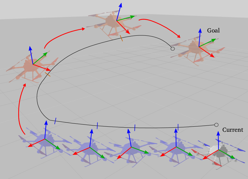
Figure 1: Illustration of the optimal trajectory computed at each time instant by the proposed approach. UAV frames represent trajectory points along the prediction horizon $T$: the blue frames represent the refined portion of the lattice, while the red ones correspond to the coarser rest of trajectory.

In this paper, we provide an effective solution to NMPC based real-time control problems, by proposing a novel adaptive time-mesh refinement strategy employed for solving the OCP, implemented inside an open-source NMPC library released with this paper.

Our approach formulates the task of steering a robot to a goal position, or along a desired trajectory, as a least square problem, where a cost over the dynamics and trajectory constraints is minimized. The optimization is performed over a discrete-time parametrization in terms of the flat outputs [7] of the dynamical system, thus decreasing the dimensionality of the OCP while reducing the computational effort required to find the solution.

In standard OCPs, an approximate solution to the continuous problem is found by discretizing the underlying control problem over a uniform time lattice. The number of discretization points is one of the major factors influencing the accuracy of the solution and the computational time: we propose to mitigate this problem by focusing also on the points location, so to condense more time samples where the discretization error is high.

We propose an algorithm that iteratively finds a suitable points distribution within the time-mesh, that satisfies a discretization error criterion. To keep the computational burden as low as possible, our approach increases the local mesh resolution only in the initial parts of the receding horizon, thus providing a higher accuracy in the section of trajectory that is more relevant to the NMPC.

We provide an open source C++ implementation of the proposed solution at:

https://bitbucket.org/gnomicSolver/gnomic

Our implementation allows to test the proposed approach on different robotic platforms, such as Unmanned Aerial Vehicles (UAVs), and ground robots, with both holonomic and non-holonomic constraints.
We exploit this implementation in our experiments, where we evaluate the proposed approach inside a simulated environment using an Asctec Firefly UAV. We proof the effectiveness of our method with a performance comparison against a standard NMPC solution.

I-A Related Work

Recently, MPC approaches have been employed in several robotics contexts [10][3][1][14][16], thanks to on-board increased computational capabilities. In [12] and [20] ACADO, a framework for fast Nonlinear Model Predictive Control (NMPC), is presented; [13] and [19] use ACADO for fast attitude control of an Unmanned Aerial Vehicle (UAV). Such a framework has been further improved in [25] by adding a code generator for embedded implementation of a linear MPC, based on an interior-point solver. Most of these methods are solving a constrained MPC problem, which is computationally complex and thus it requires a trade-off between time horizon and policy lag.

An alternative algorithm for solving unconstrained MPC problem is a Sequential Linear Quadratic (SLQ) solver. One well-known variant of SLQ called iterative Linear Quadratic Gaussian (iLQG) is presented in [24] and exhaustively tested in simulation scenarios. The feasibility of SLQ in simulation has been also confirmed in [23] and [5]. In recent works [9],[6] the authors have successfully demonstrated the effectiveness of SLQ on a real platform. However, in these projects the control is not recomputed during run time, which limits these approaches in terms of disturbance rejection, reaction to unperceived situations and imperfect state estimation. These limitations can be mitigated by solving the optimal control problem using a MPC formulation. First implementations of such approach were shown in [4] and [15]. However, in these works time horizons are short and additional tracking controllers are used instead of directly applying the feedforward and feedback gains to the actuation system. This issue has been handled in [17], where the authors allow SLQ-MPC to directly act on the actuation system, hence intrinsically improving the performance. Despite that, the size of time horizon and the number of constraints still strongly affects the computational time required for finding the solution. In [21], the authors handle this issue by exploiting the differential flatness property of under-actuated robots, like Unmanned Aerial Vehicles (UAVs). With a reduced computational effort, the solver can run at 10 Hz, thus limiting the vehicle’s capacities to safely navigate in dynamic environments. These issues are confirmed in our previous work [19], where two different NMPCs have been adopted in order to handle an Optimal Visual Servoing problem. The first serves for estimating the optimal trajectory in terms of a target re-projection error, while the second is employed as a high-level controller. The complexity introduced by the target re-projection error constraint does not allow to get a feasible solution in real-time. Hence, this does not enable the robot to successfully track moving objects.

In [18], the authors proposed an adaptive time–mesh refinement algorithm that iteratively refines the uniform lattice by adding new control points. Despite they demonstrate how the exploitation of this algorithm allows to save up to 80% runtime with respect to the uniform lattice, at the best of our knowledge, there is still no real-time implementation.

In this work we propose a Least-Square (LS) based NMPC applied to highly dynamic, non-linear dynamic robots, employing an adaptive time-mesh refinement and the differential flatness property.

The proposed time-mesh refinement procedure is similar to the one presented in [18], but with some important differences induced by the real-time application context: (i) a maximum number of refinement iteration; (ii) the usage of a discretization error as refinement criteria; (iii) the focus on the initial part of the coarse optimal trajectory.

By exploiting those properties in our efficient LS implementation, we are able to solve the NMPC problem for time horizons of multiple seconds in only a few milliseconds, obtaining unmatched performance by similar state-of-the-art algorithms. From exhaustive experiments in simulated environments, we demonstrate the capabilities of the approach in navigation tasks that leverage the full system dynamics.

I-B Contributions

The method proposed in this paper differs from previous works in the following aspects:

(i) it uses a novel adaptive time-mesh refinement algorithm that allows to reduce the computational burden, while keeping an adequate level of precision in the optimal solution; (ii) it exploits the differential flatness property of under-actuated vehicles, enabling to reduce the problem complexity; (iii) its generality allows for ease adaptation and extension to heterogeneous robotic platforms.

Moreover, we released a C++ open-source implementation for different robotic platforms.

Our claims are backed up through the experimental evaluation.

II Adaptive Finite Horizon Optimal Control

II-A Problem Statement

The goal of this work is to generate an optimal trajectory along with the set of control inputs to enable a robot to closely track it. We formulate this non-linear OCP in a NMPC fashion over the finite time horizon $T$. We assume a general non-linear time-step rule of the dynamics as

$$x_{k+1}=f(x_{k},u_{k})$$ (1)

where $x_{k}$ and $u_{k}$ denote the state vector and the control input vector at the time $t_{k}$, respectively. $f(x_{k},u_{k})$ represents the non-linear dynamic model. It is assumed to be differentiable with respect to the state $x_{k}$ and control input $u_{k}$, and it maps the state and the input vector in the subsequent time $t_{k+1}$. The time-step of the dynamics is given by $T/N$, so that each $x_{k}$ occurs at time $t_{i}=it_{f}/N$, where $N$ is the number of trajectory points used for finding the optimal solution and $t_{f}$ indicates the desired final time. The goal is to find an optimal time-varying feedback and feedforward control law of the form:

$$u(x_{k},k)=ufb(x_{k})+uff(x_{k})$$ (2)

where $uff(x_{k})$ is the feedforward term while $ufb(x_{k})$ represents the feedback control term. The optimal time-varying control law is found by iteratively finding an optimal solution for minimizing a cost function $\mathcal{C}$.

II-B Overview of the Control Framework

The cost function $\mathcal{C}$ is composed by a set of constraints over $N$ time steps of the state vector $x_{0:N}=\{x_{0},x_{1},\dots,x_{N}\}$ along with the corresponding input controls $u_{0:N-1}=\{u_{0},u_{1},\dots,u_{N-1}\}$. Defining $x_{f}$ as the desired goal state, the cost function can be formulated in a standard optimal control form as:

$$\hat{\mathcal{C}}=\frac{1}{2}\sum_{k=0}^{N-1}\left(\|x_{k}-x_{f}\|_{Q}^{2}+\|u_{k}\|_{R}^{2}\right)$$ (3)

where $\|\cdot\|_{\Omega}^{2}$ stands for the $\Omega$-norm, $Q\geq 0$ is the matrix that penalizes the distance to the goal state, and $R>0$ is the matrix weighting the control inputs. Moreover, in order to enable the solver to take advantage of the vehicle dynamic model, we add a continuity constraint between subsequent states as:

$$\mathcal{C}=\hat{\mathcal{C}}+\frac{1}{2}\sum_{k=1}^{N-1}\left(\|x_{k+1}-f(x_{k},u_{k})\|_{A_{l}}^{2}\right)$$ (4)

where the $A_{l}$ matrix weights the single state component continuity, with $A_{l}>0$. Intuitively, temporally adjacent states are forced to attain the system dynamics.

At this points, we adopt a simplifying working assumption in order to reduce the computational cost of the optimization procedure employed for minimizing the cost function stated in Eq. (4) and, therefore to handle non-linear constraints in an on-line implementation: the assumption consists of restricting our attention to non-linear differential flat systems [7]. As well-known, for such kind of systems we can find a set of outputs $\zeta\in\mathbb{R}^{m}$, named flat, of the form

$$\zeta=h(x,u,\dot{u},\cdots,u^{(r)})$$ (5)

such that there exist two functions $\psi_{k}$ and $\phi_{k}$ for which the state and the input can be expressed in terms of flat states and a finite number of their derivatives

$$x_{k}=\psi_{k}(\zeta,\dot{\zeta},\cdots,\zeta^{(c)})$$ (6)

$$u_{k}=\phi_{k}(\zeta,\dot{\zeta},\cdots,\zeta^{(c)})$$ (7)

The formulation of the OCP in terms of flat states allows for a substantial dimensionality reduction of the problem, and consequently to a saving in terms of computational cost. The cost function may consequently be rewritten using the flat outputs as

$$\hat{\mathcal{C}}(\zeta)=\frac{1}{2}\sum_{k=0}^{N-1}\left(\|\underbrace{\psi_{k}(\zeta)-x_{f}}_{\nu_{k}}\|_{Q}^{2}+\|\phi_{k}(\zeta)\|_{R}^{2}\right)$$ (8)

and, by adding also the continuity constraints, the whole cost function is calculated as

$$\mathcal{C}(\zeta)=\hat{\mathcal{C}_{0}}(\zeta)+\frac{1}{2}\sum_{k=1}^{N-1}\Bigg{(}\|\nu_{k}(\zeta)\|_{Q}^{2}+\|\phi_{k}(\zeta)\|_{R}^{2}+\\ +\|\underbrace{{\psi_{k+1}}(\zeta)-f(\psi_{k}(\zeta),\phi_{k}(\zeta))}_{\gamma_{k}}\|_{A_{l}}^{2}\Bigg{)}$$ (9)

To find the solution for the cost function in Eq. (9), we adopt a well-established numerical method for solving optimal control problems, namely direct multiple shooting [2]. In direct multiple shooting, the whole trajectory is parametrized by finite number of flat outputs $\zeta\in\mathbb{R}^{Nm}$. Hence, by stacking all the error components that compose the cost function Eq. (9), we obtain the error function $e(\zeta)$ as

$$e(\zeta)=\begin{bmatrix}\nu_{0}(\zeta)\\ \phi_{0}(\zeta)\\ \gamma_{0}(\zeta)\\ \vdots\\ \nu_{N-1}(\zeta)\\ \phi_{N-1}(\zeta)\\ \gamma_{N-1}(\zeta)\\ \end{bmatrix}$$ (10)

We minimize the error function in Eq. (10) by adopting a Least-Square iterative procedure, where the trajectory is iteratively updated as

$$\zeta\leftarrow\zeta\boxplus\delta\zeta$$ (11)

where the $\boxplus$ operator performs the variable update, while taking into account the specific composition of the flat state [22]. The update vector $\delta\zeta$ is found by solving a linear system of the form $\mathbf{H}\delta\zeta=\mathbf{b}$ with the terms $\mathbf{H}$ and $\mathbf{b}$ given by

$$\mathbf{H} = J(\zeta)^{\top}\mathbf{\Omega}J(\zeta)$$ (12)

$$\mathbf{b} = J(\zeta)^{\top}\mathbf{\Omega}e(\zeta)$$ (13)

where $J(\zeta)=\partial e(\zeta)/\partial\zeta$. To limit the magnitude of the perturbation between iterations and thus, enforce a smoother convergence, we solve a damped linear system of the form

$$\left(\mathbf{H}+\lambda\mathbf{I}\right)\delta\zeta=\mathbf{b}.$$ (14)

III ADAPTIVE TIME-MESH REFINEMENT

In non linear OCPs, the choice of the number of trajectory points $N$ is a major factor affecting the computational cost that is required to get a solution and also the accuracy of the solution itself. Hence, our goal is to effectively arrange the trajectory points along the time horizon $T$.

In this work we address the trajectory points displacement by means of an adaptive time-mesh refinement strategy. We start finding an initial solution by solving the OCP, as described in Sec. II, with a coarse lattice. Our method looks for portions of the horizon $T$ that need to be refined: we sample here new keypoints with a fine granularity.

In particular, since the NMPC employs a receding horizon strategy – where only the first trajectory point is actually used for the system actuation – we focus the resampling procedure on the initial part of the horizon.

This allows us to achieve adequate tracking performance even with a minimum amount of trajectory points $N$. As a consequence, solving more complex OCPs with longer time horizons $T$ or additional constraints (e.g. obstacles to avoid, objects to track, etc.) can be handled in real-time.

More formally, once the initial problem has been solved by employing the procedure described in Sec. II-B over an uniform time-mesh, the solution is iteratively processed. As reported in Alg. 1, at each iteration, the time-mesh refinement performs the following steps: (i) it performs a discretization error check ($\ell$. 2 and $\ell$. 12), which allows detecting where new trajectory points are required; (ii) it then adds new points by interpolating them between the adjacent ones ($\ell$. 7-8); (iii) finally, it transcribes the sub-problem into an OCP and solves it ($\ell$. 10-11). In the following, we discuss these steps in more detail.

III-A Discretization Error Check

In order to proceed with the time-mesh refinement strategy, we have to define a refinement and a stopping criteria. In this work, we consider as main refinement criterion the discretization error between the flat variables. The discretization error, at each lattice point, is computed as the difference between the current state and a higher order approximation of the solution trough the non-linear time-step rule of the dynamics of Eq. (1). More specifically, starting from the $\zeta_{k-1}$ node, we perform a finer integration of the dynamics with respect to the one employed during the OCP solution, obtaining $\hat{\zeta}_{k}$. Hence, the discretization error is computed as

$$\epsilon_{\zeta_{k}}=\|\hat{\zeta}_{k}-\zeta_{k}\|$$ (15)

where $\|\cdot\|$ stands as the squared norm of two vectors. As stopping criterion we consider a threshold on the discretization error $\epsilon_{\zeta_{k}}$.

III-B Trajectory Points Interpolation

Once the discretization error has been obtained, the time-mesh refinement proceeds by adding new trajectory nodes where required. In order to obtain a smooth interpolation that preserves the flat states differentiability, we use the cubic Hermite interpolation. More formally, let $\zeta_{i}$ and $\zeta_{j}$ be two adjacent flat states in the lattice, the interpolated flat state in the unit time interval $[0,1]$ is computed as:

$$\zeta_{k}=\zeta_{i}(2t^{3}-3t^{2}+1)+\zeta_{i}^{{}^{\prime}}(t^{3}-2t^{2}+t)\\ +\zeta_{j}(3t^{2}-2t^{3})+\zeta_{j}^{{}^{\prime}}(t^{3}-t^{2})$$ (16)

where $t\in[0,1]$ is the interpolation point, and $\zeta^{{}^{\prime}}$ denotes the first-order flat variable derivative.

III-C Local Optimization Procedure

The refinement procedure adds more node points to the initial portion of the trajectory where the discretization error is higher, so to obtain an improved solution.

As a consequence, the computational time increases. To avoid this issue, when progressively going from a coarse mesh to a refined one, the error function in Eq. (10) is scaled only to the initial part of the horizon. More specifically, let $N_{tm}=N_{i}+N_{add}$ be the number of initial trajectory points that are going to be refined, where $N_{i}<N$ is an user defined parameter representing the number of points that belong to an initial section of the trajectory, and $N_{add}$ is the number of points added at each iteration of the refinement algorithm. At each iteration, the refinement procedure transcribes these points in an OCP and re-optimizes only the mesh sub-intervals that belong to $\zeta_{0:N_{tm}}=\{\zeta_{0},\cdots,\zeta_{N_{tm}}\}$, while keeping unchanged the remaining part of the trajectory.

Data: Cost function $\mathcal{C}$, dynamics $f(x(k),u(k))$, OCP solution $\zeta_{0:N}=\{\zeta_{0},\cdots,\zeta_{N}\}$, trajectory points to refine $N_{tm}$.

Result: Refined trajectory $\zeta_{0:N+N_{add}}$

1

2scale the OCP problem: $\zeta_{0:N_{tm}}=\{\zeta_{0},\cdots,\zeta_{N_{tm}}\}$;

3 discretization error computation for each lattice point $\epsilon_{\zeta_{1:N_{tm}}}$;

4 $iter=0$;

5while $iter<max_{iter}$ do

6       foreach $\zeta_{i}\in\zeta_{1:N_{tm}}$ do

7             if  $\epsilon_{\zeta}>err_{trs}$  then

8                   $\zeta_{k}=Interpolate(\zeta_{i},\zeta_{i+1})$;

9                   Add $\zeta_{k}$ to $\zeta_{0:N_{tm}}$;

10                   $N_{tm}\leftarrow N_{tm}+1$;

11                  

12             transcribe the scaled OCP;

13             apply the Least-Square solver;

14             estimate the discretization error $\epsilon_{\zeta_{1:N_{tm}}}$;

15             $iter\leftarrow iter+1$;

16            

17       end foreach

18      

19 end while

Algorithm 1 Time-Mesh Refinement Algorithm.

TABLE I: Errors and Control Inputs Statistics for the Pose Regulation Experiment

	$N$	$TMref$	$Runtime[ms]$	$err_{trans}[m]$	$err_{rot}[rad]$	$Roll_{ref}[rad]$	$Pitch_{ref}[rad]$	$YawRate[rad/s]$	$Thrust[Nm]$
	100		42	0.0537	0.0435	0.0196	0.0196	0.3305	15.2450
	50		10	0.0613	0.0543	0.0184	0.0210	0.2906	15.1695
	50	✓	10.2	0.0608	0.0521	0.0191	0.0213	0.2863	15.2237
	20		1	0.0724	0.0598	0.0195	0.0259	0.3146	15.1554
	20	✓	1.2	0.0703	0.0553	0.0193	0.0224	0.2929	15.2491
	10		0.5	0.1096	0.0735	0.0207	0.0257	0.2964	15.1352
	10	✓	0.7	0.0823	0.0642	0.0197	0.0243	0.3321	15.1934
	5		0.2	fail	fail	fail	fail	fail	fail
	5	✓	0.4	0.1032	0.0667	0.0219	0.0234	0.3219	15.2154

IV Experimental Evaluation

We tested the proposed approach in a simulated environment by using the RotorS simulator [8] and a multirotor model. The mapping between the high-level control input and the propeller velocities is done by a low-level PD controller that aims to resemble the low-level controller that runs on a real multirotor.

The evaluation presented here is designed to support the claims made in the introduction. We performed two kind of experiments, namely pose regulation and trajectory tracking.

We provide a direct comparison between a standard NMPC implementation and the one presented in this paper, i.e. by using a time-mesh refinement strategy.

We formulate the OCP by composing each flat state of the UAV simulated model as follows:

$$\begin{array}[]{ccc}\zeta=(p_{1},p_{2},p_{3},\gamma)\end{array}$$ (17)

where $p_{i}$ is the translation in the world coordinate reference system along the $i^{th}$ axis, and $\gamma$ represents the yaw angle. For more detail about the dynamical model and the flat model, please refer to Appendix A.

IV-A Pose Regulation

We disegned the following pose regulation experiment to prove the accuracy and the robustness of the proposed approach. In all the regulation experiments we set the desired state to be:

$$\begin{array}[]{ccc}t_{f}=2,&\zeta=(2,2,1,1.57),&\dot{\zeta}=(0,0,0,0).\end{array}$$

and the time-mesh refinement parameters to be $err_{trs}~{}=~{}10^{-5},\quad max_{iter}=2.$

The pose regulation tasks are performed while varying the bins number $N$. Our goal is to show how the control accuracy deteriorates while going from a finer lattice to a coarser one. To this end, we started with $N=200$, that we used as a reference for the other bin setups. We decreased the bins amount up to $N=5$ measuring the translational and rotational RMSE with respect to the reference trajectory, for both the standard NMPC case and our approach. We report the results of this comparison in Tab. I, along with the computational time required for solving the OCP and the control inputs average.

The advantages of using a time-mesh refinement strategy are twofold. From one side, when using a coarse lattice, as in the case of $N=20$ and $N=10$, the refined solution provides lower errors, with a negligible increment of computational time. On the other hand, it intrinsically increases the robusteness by adaptively adding bins in the trajectory where needed, thus avoiding failures such as the one registerd with $N=5$ in the standard NMPC formulation. Fig. 2 directly compares the convergence with the reference trajectory ($N=200$) and the ones recorded while using $N=20$ and $N=5$ with the time-mesh refinement.

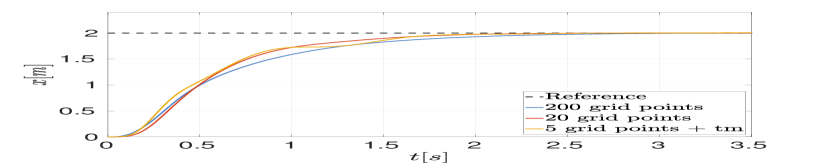
(a) x-coord error

(b) y-coord error

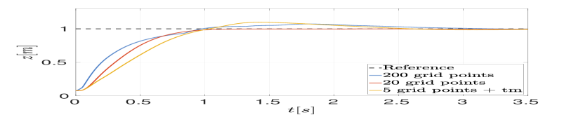
(c) z-coord error

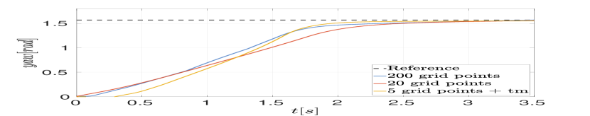
(d) yaw error

Figure 2: Pose Error

IV-B Trajectory Tracking

To prove the effectiveness of the proposed time-mesh refinement in a tracking scenario, we command the UAV platform to track a challenging Lemniscate trajectory, defined by the following expression:

$$p_{1}(t) =2sin(t/2)$$

$$p_{2}(t) =2sin(t/2)cos(t/2)$$

$$p_{3}(t) =sin(t+5)/3$$

$$\gamma(t) =sin(t/8)$$

We set $t_{f}=0.5s$ and $N=5$ for both the standard and the refined setup, while we set $err_{trs}$ and $max_{iter}$ with the same values used in the pose regulation section IV-A. We report the results of the tracking experiments in Fig. 3(a) and Fig. 4(a). As expected, the use of a time-mesh refinement strategy allows for a more accurate tracking since the OCP problem is solved over an adapted lattice.

IV-C Runtime

We recorded the time needed to solve the NMPC problem, as described in Sec. II. We performed all the presented experiments on a laptop computer equipped with a i7-5700HQ CPU with 2.70 GHz. Our software runs on a single core and in a single thread.

To reduce the noise in the measurements, we collect the computational times for time horizons between $500ms$ and $4000ms$, using bins of $200ms$. For each configuration of the solver, we compute the average computational time over 4000 planned trajectories with an UAV, and report these values in Fig. 5.

As shown in Fig. 5, while increasing the time horizon, and consequently the number of bins, the computational time grows almost linearly. The computational overhead of the time-mesh refinement, in this sense, does not affect such a cost, by adding a constant time to the total computation.

Fig. 6 shows the runtime percentage in case of $t_{f}=2s$ with bins each $200ms$, where the time-mesh refinement slice includes the computational time involved in all the different mesh refinement steps. Note that the time-mesh refinement portion has constant time consumption. Thus its percentage value is indicative of this particular setup only. It is also noteworthy to highlight how most of the runtime is absorbed by the Jacobian calculation, being computed in a fully numerical manner.

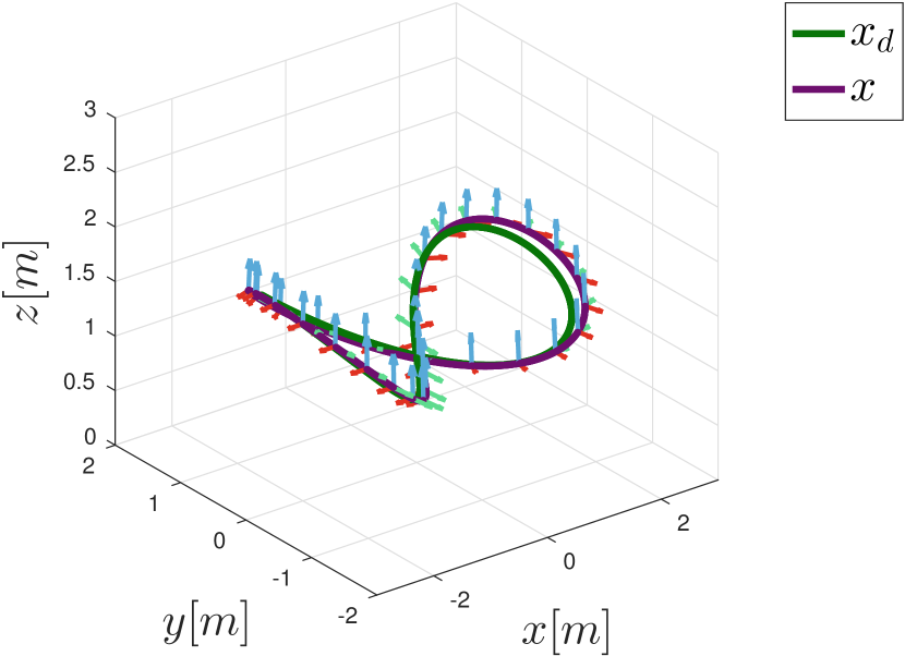
(a) Trajectory Tracking.

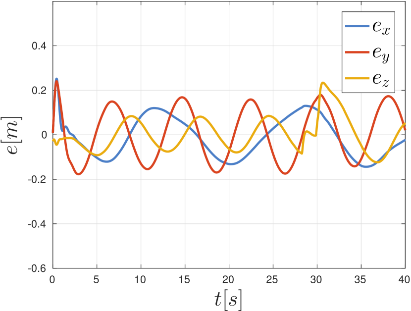
(b) Position Error.

Figure 3: Lemniscate trajectory tracked with standard approach.

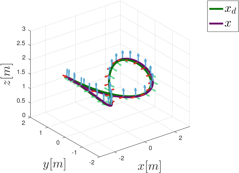
(a) Trajectory Tracking.

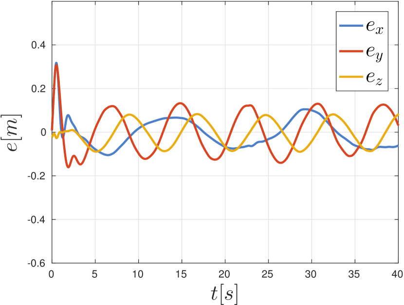
(b) Position Error.

Figure 4: Lemniscate trajectory tracked with time-mesh refinement.

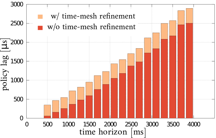
Figure 5: Average runtime over 4000 planned trajectories with horizon up to $4s$, with an UAV model.

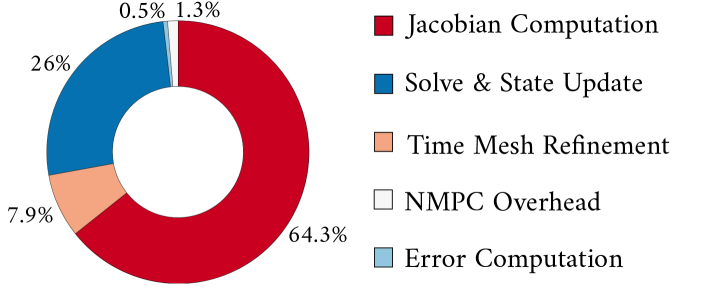
Figure 6: Runtime percentage of the NMPC algorithm with time-mesh refinement in case of $t_{f}=2s$ with bins each $200ms$.

V Conclusion

In this paper, we present a novel solution for real-time NMPC employing a time-mesh refinement strategy. We addressed the planning and tracking problems in an unified manner by solving a least-squares optimization formulation, over the flat outputs of the controlled system. We evaluated our approach through regulation and tracking experiments with an UAV simulated platform. The experiments suggest that the proposed time-mesh refinement allows to improve the accuracy of the solution enabling better control performances, without significantly increasing the computational effort. We release our C++ open-source implementation, enabling to test the proposed algorithm with different robotic platforms. As a future work, we will investigate additional error constraints over longer horizons.

Appendix A Differential Flatness for UAV

Let $\mathnormal{F}_{I}$ be the right-hand inertial reference frame with unit vectors along the axes denoted by $\{\vec{\mathbf{i}}_{x},\vec{\mathbf{i}}_{y},\vec{\mathbf{i}}_{z}\}$. The vector $p=(p_{1},p_{2},p_{3})\in\mathnormal{F}_{I}$ denotes the position of the center of mass of the vehicle.

Let $\mathnormal{F}_{B}$ be the right-hand body reference frame with unit vectors $\{\vec{\mathbf{b}}_{x},\vec{\mathbf{b}}_{y},\vec{\mathbf{b}}_{z}\}$, where these vectors are the axes of frame $\mathnormal{F}_{B}$ with respect to frame $\mathnormal{F}_{I}$. The orientation of the rigid body is given by the rotation ${{}^{I}R_{B}}=R=\begin{bmatrix}\vec{\mathbf{b}}_{x}&\vec{\mathbf{b}}_{y}&\vec{\mathbf{b}}_{z}\end{bmatrix}\in\mathit{SO}(3)$.

Let $\mathit{v}\in\mathnormal{F}_{I}$ express the linear velocity of the body, expressed in the inertial reference frame $\mathnormal{F}_{I}$. Let $\mathit{\omega}\in\mathnormal{F}_{B}$ be the angular velocity of the body with respect to $\mathnormal{F}_{I}$. Let $\mathit{m}$ denote the mass of the rigid body, and $\mathbf{I}\in{}^{3x3}$ the constant inertia matrix expressed in body frame, the rigid body equations can be expressed as

$$\dot{\xi}=\mathit{v},$$ (18a)

$$\mathit{m}\dot{v}=\mathit{m}\mathit{g}\vec{\mathbf{i}}_{z}+RF_{t}$$ (18b)

$$\dot{R}=R~{}\mathit{\omega}_{\times}$$ (18c)

$$\mathbf{I}\dot{\mathit{\omega}}=-\mathit{\omega}\times\mathbf{I}\mathit{\omega}+\tau$$ (18d)

where the notation $\mathit{\omega}_{\times}$ denotes for the skew-symmetric matrix formed from $\mathit{\omega}$. The system inputs $F_{t},\tau\in\mathnormal{F}_{B}$ act respectively as thrust force and body torques. The system reported in Eq. (18) can be represented exploiting the differential flatness property. For an UAV underactuated vehicle, the flat outputs are given as $\zeta=(p_{1},p_{2},p_{3},\gamma)\in{}^{4}$, where $\gamma$ represents the yaw angle. Hence, by denoting $p_{t}=(p_{1},p_{2},p_{3})$, we recover the full state and controls by using the following relations: $p=p_{t}$, $\dot{p}=\dot{p_{t}}$, $F_{t}=\|\mathit{m}(\ddot{p_{t}}-\mathit{g})\|$ and the three columns of the rotation matrix $R$ as:

$$R_{z}=\mathit{m}(\ddot{p_{t}}-\mathit{g})/F_{t}$$

$$R_{y}=R_{z}\times\begin{pmatrix}cos~{}\mathit{\gamma_{t}}\\ sin~{}\mathit{\gamma_{t}}\\ 0\end{pmatrix}/\Bigg{\|}R_{z}\times\begin{pmatrix}cos~{}\mathit{\gamma_{t}}\\ sin~{}\mathit{\gamma_{t}}\\ 0\end{pmatrix}\Bigg{\|}$$

$$R_{x}=R_{y}\times R_{z}.$$

The angular velocity is recovered as

$$\mathit{\omega}_{x}=-R_{y}~{}\dddot{p_{t}}/F_{t}$$

$$\mathit{\omega}_{y}=R_{x}~{}\dddot{p_{t}}/F_{t}$$

$$\mathit{\omega}_{z}=\dot{\mathit{\gamma_{t}}}~{}(\vec{\mathbf{i}}_{z}~{}R_{z})$$

where $\vec{\mathbf{i}}_{z}$ is the standard unit vector along the z-axis. To recover $\tau$, we first recover $\dot{\mathit{\omega}}$. Note that from the dynamics

$$\mathit{m}~{}p_{t}^{(4)}=(R\hat{\mathit{\omega}}^{2}+R\hat{\dot{\mathit{\omega}}})F_{t}~{}\vec{\mathbf{i}}_{z}+2~{}R~{}\hat{\mathit{\omega}}\dot{F_{t}}\vec{\mathbf{i}}_{z}+R~{}\ddot{F_{t}}~{}\vec{\mathbf{i}}_{z}$$

Solving this for $\dot{\mathit{\omega}}$ gives

$$\mathit{\omega}_{x}=(-\mathit{m}R_{y}~{}p_{t}^{(4)}-\mathit{\omega}_{y}\mathit{\omega}_{z}F_{t}+2\mathit{\omega}_{x}\dot{F_{t}})/F_{t}$$

$$\mathit{\omega}_{y}=(\mathit{m}R_{y}~{}p_{t}^{(4)}-\mathit{\omega}_{x}\mathit{\omega}_{z}F_{t}-2\mathit{\omega}_{y}\dot{F_{t}})/F_{t}$$

$$\mathit{\omega}_{z}=\ddot{\gamma_{t}}\vec{\mathbf{i}}_{z}~{}R_{z}+\dot{\gamma_{t}}\vec{\mathbf{i}}_{z}^{T}R\hat{\mathit{\omega}}\vec{\mathbf{i}}_{z}$$

Then we use the dynamics $\tau=\mathbf{I}\dot{\mathit{\omega}}-\mathbf{I}\mathit{\omega}\times\mathit{\omega}$ and $\tau$ is recovered.

References

- [1] K. Alexis, C. Papachristos, G. Nikolakopoulos, and A. Tzes. Model predictive quadrotor indoor position control. In Proc. of the Mediterranean Conf. on Control Automation (MED), pages 1247–1252, 2011.
- [2] John T Betts. Survey of numerical methods for trajectory optimization. Journal of Guidance control and dynamics, 21(2):193–207, 1998.
- [3] P. Bouffard, A. Aswani, and C. Tomlin. Learning-based model predictive control on a quadrotor: Onboard implementation and experimental results. In Proc. of the IEEE Intl. Conf. on Robotics & Automation (ICRA), pages 279–284, May 2012.
- [4] T. Erez, S. Kolev, and E. Todorov. Receding-horizon online optimization for dexterous object manipulation. preprint avbl online, 2014.
- [5] Tom Erez, Yuval Tassa, and Emanuel Todorov. Infinite-horizon model predictive control for periodic tasks with contacts. In Proc. of Robotics: Science and Systems (RSS), Los Angeles, CA, USA, 2011.
- [6] Farbod Farshidian, Michael Neunert, and Jonas Buchli. Learning of closed-loop motion control. In Proc. of the IEEE/RSJ Intl. Conf. on Intelligent Robots and Systems (IROS), pages 1441–1446. IEEE, 2014.
- [7] Michel Fliess, Jean Lévine, Philippe Martin, and Pierre Rouchon. Flatness and defect of non-linear systems: introductory theory and examples. International journal of control, 61(6):1327–1361, 1995.
- [8] Fadri Furrer, Michael Burri, Markus Achtelik, and Roland Siegwart. Robot Operating System (ROS): The Complete Reference (Volume 1), chapter RotorS—A Modular Gazebo MAV Simulator Framework, pages 595–625. Springer International Publishing, 2016.
- [9] G. Garimella and M. Kobilarov. Towards model-predictive control for aerial pick-and-place. In Proc. of the IEEE Intl. Conf. on Robotics & Automation (ICRA), pages 4692–4697, May 2015.
- [10] R. Ginhoux, JA Gangloff, MF De Mathelin, L. Soler, M. Sanchez, and J. Marescaux. Beating heart tracking in robotic surgery using 500 hz visual servoing, model predictive control and an adaptive observer. In Proc. of the IEEE Intl. Conf. on Robotics & Automation (ICRA), volume 1, pages 274–279. IEEE, 2004.
- [11] Lars Grüne and Jürgen Pannek. Nonlinear model predictive control. In Nonlinear Model Predictive Control. Springer, 2017.
- [12] B. Houska, HJ Ferreau, and M. Diehl. ACADO toolkit—an open-source framework for automatic control and dynamic optimization. Optimal Control Applications and Methods, 32(3):298–312, 2011.
- [13] M. Kamel, K. Alexis, M. Achtelik, and R. Siegwart. Fast nonlinear model predictive control for multicopter attitude tracking on so(3). In IEEE Conference on Control Applications (CCA), 2015.
- [14] Nima Keivan and Gabe Sibley. Realtime simulation-in-the-loop control for agile ground vehicles. In Conference Towards Autonomous Robotic Systems, pages 276–287. Springer, 2013.
- [15] J. Koenemann, A. Del Prete, Y. Tassa, E. Todorov, O. Stasse, M. Bennewitz, and N. Mansard. Whole-body model-predictive control applied to the hrp-2 humanoid. In Proc. of the IEEE/RSJ Intl. Conf. on Intelligent Robots and Systems (IROS), pages 3346–3351. IEEE, 2015.
- [16] Alexander Liniger, Alexander Domahidi, and Manfred Morari. Optimization-based autonomous racing of 1:43 scale rc cars. Optimal Control Applications and Methods, 36(5):628–647, 2015.
- [17] M. Neunert, C. de Crousaz, F. Furrer, M. Kamel, F. Farshidian, R. Siegwart, and J. Buchli. Fast nonlinear model predictive control for unified trajectory optimization and tracking. In Proc. of the IEEE Intl. Conf. on Robotics & Automation (ICRA), pages 1398–1404, 2016.
- [18] Luís Tiago Paiva and Fernando ACC Fontes. Sampled–data model predictive control using adaptive time–mesh refinement algorithms. In CONTROLO 2016, pages 143–153. Springer, 2017.
- [19] C. Potena, D. Nardi, and A. Pretto. Effective target aware visual navigation for UAVs. In Proc. of the Europ. Conf. on Mobile Robotics (ECMR), Sept 2017.
- [20] R. Quirynen, M. Vukov, M. Zanon, and M. Diehl. Autogenerating microsecond solvers for nonlinear mpc: A tutorial using acado integrators. Optimal Control Applications and Methods, 36(5), 2015.
- [21] M. Sheckells, G. Garimella, and M. Kobilarov. Optimal visual servoing for differentially flat underactuated systems. In Proc. of the IEEE/RSJ Intl. Conf. on Intelligent Robots and Systems (IROS), 2016.
- [22] R. Smith and P. Cheeseman. On the representation and estimation of spatial uncertainty. The international journal of Robotics Research, 5(4):56–68, 1986.
- [23] Y. Tassa, T. Erez, and E. Todorov. Synthesis and stabilization of complex behaviors through online trajectory optimization. In Proc. of the IEEE/RSJ Intl. Conf. on Intelligent Robots and Systems (IROS), pages 4906–4913, 2012.
- [24] E. Todorov and W. Li. A generalized iterative LQG method for locally-optimal feedback control of constrained nonlinear stochastic systems. In Proc. of the IEEE American Control Conference (ACC), 2005.
- [25] M. Vukov, A. Domahidi, HJ Ferreau, M. Morari, and M. Diehl. Auto-generated algorithms for nonlinear model predictive control on long and on short horizons. In Decision and Control (CDC), IEEE Conference on, pages 5113–5118, 2013.