Streamline integration as a method for structured grid generation in X-point geometry

Abstract

We investigate structured grids aligned to the contours of a two-dimensional flux-function with an X-point (saddle point). Our theoretical analysis finds that orthogonal grids exist if and only if the Laplacian of the flux-function vanishes at the X-point. In general, this condition is sufficient for the existence of a structured aligned grid with an X-point. With the help of streamline integration we then propose a numerical grid construction algorithm. In a suitably chosen monitor metric the Laplacian of the flux-function vanishes at the X-point such that a grid construction is possible.

We study the convergence of the solution to elliptic equations on the proposed grid. The diverging volume element and cell sizes at the X-point reduce the convergence rate. As a consequence, the proposed grid should be used with grid refinement around the X-point in practical applications. We show that grid refinement in the cells neighbouring the X-point restores the expected convergence rate.

1 Introduction

A magnetic X-point is particularly advantageous for the confinement of particles and thermal energy inside a magnetic fusion device [1]. For this reason, two- and three-dimensional simulations that encompass the X-point in the cross-section of magnetically confined fusion plasmas have emerged in past years [2, 3, 4, 5, 6, 7, 8, 9, 10, 11, 12]. There, so-called flux-surfaces [1] bound the idealized toroidally symmetric physical domain. Analytically, the flux-surfaces are represented by the contour lines of the flux-function $\psi$, which at an X-point has a vanishing gradient and an indefinite Hessian matrix. It has proven advantageous to use grid points that align with this flux-function in numerical simulations. This is especially true in the closed field line region, where flux-aligned structures like zonal flows regulate the turbulent transport [13]. Furthermore, once the domain of interest is bounded by flux-surfaces, a ”flux-aligned” grid allows for an easy treatment of boundary conditions.

Unfortunately, structured grids (grids generated by a coordinate transformation) aligned to flux-surfaces may lead to numerical issues when an X-point is present in the domain. This is because one coordinate of a structured aligned grid is necessarily the flux-function $\psi$ itself or a monotonous function of it. Since $\psi$ has per definition a saddle point with $\nabla\psi=0$, the Jacobian of the coordinate transformation vanishes at this point and the transformation becomes singular. This also entails vanishing or diverging elements in the metric tensor, which appear in the physical equations transformed to the new coordinate system and therefore enter the numerical discretization. However, these issues do not directly manifest in the grid points themselves. In fact, with the help of streamline integration [14, 15] it is fairly straightforward to numerically construct grid points that are aligned with the flux-surfaces. What is unclear is whether

• these then actually represent a (homeomorphic) coordinate transformation,

• a numerical scheme can cope with the singularity (consistence),

• the convergence rate of a numerical scheme is affected by the singularity.

For example, in an elliptic equation the solution depends on all points in the domain and we cannot a priori know whether singular points reduce or prevent the global convergence rate of the solution. We are the first to address these concerns, which have not been studied systematically in the literature so far. Nevertheless, results from simulations on structured aligned grids have already been published [9, 10, 11, 12] without investigating or solving the above issues. We believe that the therein presented conclusions require a discussion in the light of the numerical uncertainties and the results in the present article.

Let us mention that, of course, the use of coordinate patches or entirely unstructured grids is always possible and circumvents the problem [4, 16, 17, 18]. Still, we investigate the use of structured grids in this contribution as they have several advantages. First of all, numerical methods on structured grids are very easily implemented. Unstructured coordinate patches introduce an overhead due to the additional bookkeeping induced by the explicit topological information of grid patches or cells. Furthermore, this overhead necessarily leads to a loss in performance over structured grids since for example in the computation of derivatives the additional topological information needs to be separately loaded from the system memory. This is detrimental for memory bandwidth bound problems.

For completeness let us also mention recent approaches to use non flux-aligned grids for the discretization of model equations [19, 20, 21]. Like unstructured grids, these avoid numerical issues with the X-point but shift the problem to the question of how to correctly implement a flux-aligned boundary.

Finally, let us note that even though we motivated the problem from within the field of magnetic confinement fusion, its nature is purely mathematical. Our results therefore apply to any situation in which an alignment of a numerical grid to a two-dimensional function with X-point is desirable. Also note that in this contribution the discussion of O-points (extrema of the flux-function) is missing. This is because we assume the Hessian matrix of the flux-function to be indefinite in our derivation and the results therefore do not apply to O-points.

In this contribution we investigate how structured grids can be consistently constructed and how numerical methods behave when there is an X-point present in the computational domain. In Section 2 we discuss general properties of structured grids aligned to flux-surfaces from an analytical point of view. We derive a consistency equation that all structured grids aligned to a flux-function have to obey. Based on this we derive necessary and sufficient conditions to fulfil this equation. We then propose a grid generation algorithm for orthogonal grids in Section 3. Our algorithm is based on streamline integration [14, 15] and assumes that the Laplacian of the flux-function vanishes at the X-point. This technique allows the efficient computation of grid coordinates as well as the corresponding Jacobian and therefore metric elements up to machine precision. We pay special attention to the discretization of the separatrix (the contour line through the X-point). In the following Section 4 we then show how our algorithm applies to cases with a non-vanishing Laplacian at the X-point. We introduce the concept of a monitor metric. Finally, in Section 5 we apply our algorithm first to an analytical example and second to a practical problem taken from the field of magnetically confined fusion. With the analytical example we in particular show how grid generation algorithms fail without monitor metric. For the second case we solve an elliptic equation on our generated grid and show convergence rates of a local discontinuous Galerkin discretization of various order [22]. If the solution varies across the X-point, we need grid refinement to restore the convergence of our solution, which otherwise deteriorates to order one in the cell-size due to the diverging volume element.

2 Structured grids with X-point

Given is a two-dimensional flux-function $\psi(x,y)$ in some coordinates $x$ and $y$. At one point $x_{X},y_{X}$ this function has a saddle point (the X-point), where the gradient vanishes and the Hessian matrix is indefinite. Let us assume the existence of a metric tensor $g$ with elements given in the coordinates $x$ and $y$. We now express a coordinate system $\zeta,\eta$ with $\zeta$ aligned to $\psi(x,y)$ as

$$\mathrm{d}\zeta =f(\psi)(\psi_{x}\mathrm{d}x+\psi_{y}\mathrm{d}y)$$ (1a)

$$\mathrm{d}\eta =a(x,y)\sqrt{g}[-\psi^{y}\mathrm{d}x+\psi^{x}\mathrm{d}y]-b(x,y)[\psi_{x}\mathrm{d}x+\psi_{y}\mathrm{d}y]$$ (1b)

Equation (1a) expresses the alignment property $\mathrm{d}\zeta=f(\psi)\mathrm{d}\psi$ with $f(\psi)\neq 0$. Our choice for the form of $\mathrm{d}\eta$ in Eq. (1b) becomes apparent further down in the text. It is a re-expression of the general exact 1-form in two dimensions, $\mathrm{d}\eta=\eta_{x}\mathrm{d}x+\eta_{y}\mathrm{d}y$. In place of $\eta_{x}$ and $\eta_{y}$ we introduce the two free functions $a(x,y)\neq 0$ (if $f$ or $a$ were zero at a point, the coordinate transformation would become singular) and $b(x,y)$. We have the contravariant components of $\nabla\psi$,

$$\psi^{x}:=g^{xx}\psi_{x}+g^{xy}\psi_{y},\quad\psi^{y}:=g^{xy}\psi_{x}+g^{yy}\psi_{y}$$

and the element of the volume form $\sqrt{g}:=(g_{xx}g_{yy}-g_{xy}g_{xy})^{1/2}$. Then, $\eta_{x}=-\sqrt{g}\psi^{y}a-\psi_{x}b$ and $\eta_{y}=\sqrt{g}\psi^{x}a-\psi_{y}b$, which is invertible for $a$ and $b$ if $(\nabla\psi)^{2}=\psi^{x}\psi_{x}+\psi^{y}\psi_{y}\neq 0$. In fact, we then have

$$a=\frac{\psi_{x}\eta_{y}-\psi_{y}\eta_{x}}{\sqrt{g}(\nabla\psi)^{2}},\quad b=-\frac{\psi^{x}\eta_{x}+\psi^{y}\eta_{y}}{(\nabla\psi)^{2}}.$$ (2)

Recall the familiar rules for tensor transformation (e.g. [23]). The elements of the inverse metric tensor $g^{-1}$ in the transformed coordinates read

$$\left.\begin{pmatrix}\bar{g}^{\zeta\zeta}&\bar{g}^{\zeta\eta}\\ \bar{g}^{\eta\zeta}&\bar{g}^{\eta\eta}\end{pmatrix}\right|_{\zeta(x,y),\eta(x,y)}=\left(\nabla\psi\right)^{2}\left.\begin{pmatrix}f^{2}&-bf\\ -bf&a^{2}+b^{2}\end{pmatrix}\right|_{x,y},\quad\sqrt{\bar{g}}^{\,-1}=(\nabla\psi)^{2}af,$$ (3a)

which shows that we obtain an orthogonal grid (a grid in which the base vectors are orthogonal in the given metric) with $b=0$. We denote $\bar{g}^{ij}$ as the elements of $g^{-1}$ in the transformed coordinate system $\zeta,\eta$ and analogous $\sqrt{\bar{g}}$ the element of the volume form in transformed coordinates.

Let us emphasize here that the metric tensor $g$ is not necessarily the canonical, Cartesian metric. We only assume that $g$, as well as the coordinates $x$ and $y$, are well-defined and do not expose any singularities. Further note that our choice of notation is based on differential forms rather than what is traditionally used in the plasma physics literature [14]. In this way the relation between the metric tensor and the more fundamental objects (covariant and contravariant base vectors) is disentangled. This becomes advantageous in Sections 3 and 4, where we want to freely choose the metric tensor.

Now, we place ourselves in a reverse position. If $\psi$ and the metric $g$ are given, is it possible to find $\zeta$ and $\eta$ in the form presented in Eq. (1)? In fact, this question is equivalent to finding conditions for the functions $a$, $b$ and $f$ such that the right-hand sides of Eqs. (1a) and (1b) are exact forms. Recall that the Poincaré lemma states that a closed form is exact [23]. Therefore, $f\mathrm{d}\psi$ has a potential $\zeta$ if $\mathrm{d}(f\mathrm{d}\psi)=0$. This results in

$$f_{y}\psi_{x}-f_{x}\psi_{y}=0$$

and is fulfilled if $f$ is a function of $\psi$ only. In order for the coordinate $\eta$ to exist it must hold that $\mathrm{d}[(-a\sqrt{g}\psi^{y}-b\psi_{x})\mathrm{d}x+(\sqrt{g}\psi^{x}a-\psi_{y}b)\mathrm{d}y]=0$. In coordinates that is

$$\frac{\partial}{\partial x}\left(\sqrt{g}a\psi^{x}-b\psi_{y}\right)+\frac{\partial}{\partial y}\left(\sqrt{g}a\psi^{y}+b\psi_{x}\right)=0.$$

This can be rewritten to

$$a\Delta\psi+\nabla\psi\cdot\nabla a+\{\psi,b\}=0,$$ (4)

where $\Delta\psi$ is the Laplacian operator given by

$$\Delta\psi:=\frac{1}{\sqrt{g}}\left(\frac{\partial}{\partial x}\left(\sqrt{g}\psi^{x}\right)+\frac{\partial}{\partial y}\left(\sqrt{g}\psi^{y}\right)\right)$$ (5)

and we identified the Poisson bracket

$$\{\psi,b\}:=\frac{1}{\sqrt{g}}(\psi_{x}b_{y}-\psi_{y}b_{x}).$$

It is the recovery of the Laplacian, the gradient and the Poisson bracket in Eq. (4) that justifies our choice of Eq. (1b).

Since the flux-function $\psi(x,y)$ and the metric $g$ are given, Eq. (4) is a constraint on the functions $a(x,y)$ and $b(x,y)$. We call Eq. (4) the consistency equation and for the remainder of this section we focus on its implications. Apparently, the problematic point is the X-point, where $\psi_{x}$ and $\psi_{y}$ vanish, but $\Delta\psi$ might not. We therefore ask under what circumstances well-defined solutions $a$ and $b$ exist, depending on the properties of $\psi$ at the X-point. A vanishing Laplacian is in fact a very desirable quality of $\psi$. At this point an example is instructive.

Example 1.

We consider $\psi=\tfrac{1}{2}(x^{2}-y^{2})$ and $f(\psi)=1$ in the canonical (Cartesian) metric, for which $\Delta\psi=0$. One possible choice for the second coordinate is $\eta=xy$. Equation (2) yields at once $a=1$ and $b=0$ that is, we have obtained an orthogonal coordinate system ($b=0$). The non-zero metric elements are $\bar{g}^{\zeta\zeta}=\bar{g}^{\eta\eta}=x^{2}+y^{2}$ from which we can compute the volume element $\sqrt{\bar{g}}=1/(x^{2}+y^{2})$.

It turns out that $\Delta\psi=0$ at the X-point is sufficient for the existence of well-defined $a$ and $b$ solving Eq. (4). We prove this by actually constructing an algorithm in Section 3.

The following theorem shows what a vanishing Laplacian means in geometrical terms. Without loss of generality we assume $\psi(x_{X},y_{X})=0$ and call the curve given implicitly by $\psi(x,y)=0$ the separatrix.

Theorem 1.

If $\Delta\psi|_{x_{X},y_{X}}=0$ in a given metric $g$, then the tangent vectors to the separatrix are orthogonal at the X-point in this metric.

Proof.

Let us expand $\psi$ around the X-point

$$\psi(x,y)=\frac{1}{2}(x-x_{X},y-y_{X})^{\mathrm{T}}\left.\begin{pmatrix}\psi_{xx}&\psi_{xy}\\ \psi_{xy}&\psi_{yy}\end{pmatrix}\right|_{x_{X},y_{X}}\begin{pmatrix}x-x_{X}\\ y-y_{X}\end{pmatrix}+\dots$$

Neglecting higher order terms the equation $\psi(x,y)=0$ then yields a quadratic equation for $x-x_{X},y-y_{X}$ with the two solution vectors

$${\mathbf{s}}_{1,2}=\left.\begin{pmatrix}-\psi_{xy}\pm\sqrt{\psi_{xy}^{2}-\psi_{xx}\psi_{yy}}\\ \psi_{xx}\end{pmatrix}\right|_{x_{X},y_{X}}.$$

Now we use that the Laplacian of $\psi$ in the metric $g$ vanishes at the X-point

$$g^{xx}\psi_{xx}+2g^{xy}\psi_{xy}+g^{yy}\psi_{yy}=0,$$

where we used that $\psi_{x}=\psi_{y}=0$ at the X-point. With this we can readily compute $\sum_{ij=1}^{2}g_{ij}s_{1}^{i}s_{2}^{j}=0$ that is ${\mathbf{s}}_{1}$ and ${\mathbf{s}}_{2}$ are perpendicular at the X-point in the metric $g$. ∎

Now, we can of course ask what happens if $\Delta\psi\neq 0$ at the X-point. The first observation we make is that for such a non-orthogonal X-point no coordinate system can exist such that $a$ and $b$ as well as their derivatives are bounded.

Theorem 2.

If $a$ and $b$ as well as their derivatives are bounded, then it must hold that $\Delta\psi=0$ at the X-point.

Proof.

Since $\psi_{x}=\psi_{y}=0$ at the X-point, Eq. (4) gives $a\Delta\psi=0$. For $a\neq 0$ this can only be satisfied if $\Delta\psi=0$. ∎

Let us now turn our attention to the case in which either $a$ or $b$ is allowed to diverge at the X-point. Special cases worth investigating are $a=1$ as in the grid proposed by [24] and $b=0$, which yields an orthogonal grid. It turns out that $\Delta\psi=0$ at the X-point is also a necessary condition for well-defined $a$ and $b$ to exist in these cases:

Theorem 3.

If $\psi$ is a smooth function on a bounded domain that includes a non-orthogonal X-point with $\Delta\psi\neq 0$, then there exists no flux-aligned coordinate system $(\zeta,\eta)$ for which $a=1$ and $b$ is well defined at the X-point. Analogously there exists no flux-aligned coordinate system for which $b=0$ and $a$ is well defined at the X-point.

Proof.

Substituting $a=1$ into equation (4) gives

$$\{\psi,b\}=-\Delta\psi$$

and thus

$$-\psi_{y}b_{x}+\psi_{x}b_{y}=-\sqrt{g}\Delta\psi.$$

By the method of characteristics we obtain curves $x(t)$, $y(t)$, and $b(t)$ such that

$$\dot{x}(t)=-\psi_{y}(x(t),y(t)),\qquad\dot{y}(t)=\psi_{x}(x(t),y(t)),\qquad\dot{b}=-\sqrt{g}\Delta\psi(x(t),y(t)).$$

This implies

$$b(t)=b(0)-\int_{0}^{t}\sqrt{g}\Delta\psi(x(t^{\prime}),y(t^{\prime}))\,\mathrm{d}t^{\prime}.$$

Without loss of generality we assume that the X-point is located at $(0,0)$ and that $\Delta\psi(0,0)>0$. Now, we consider characteristics curves $(x_{1}(t),y_{1}(t))$ and $(x_{2}(t),y_{2}(t))$ such that $\lim_{t\to\infty}(x_{1}(t),y_{1}(t))=0$ and $\lim_{t\to-\infty}(x_{2}(t),y_{2}(t))=0$. Then $b(0,0)=\lim_{t\to\infty}b_{1}(t)=-\infty$ and $b(0,0)=\lim_{t\to-\infty}b_{2}(t)=\infty$. Thus, we have obtained a contradiction. The proof for $b=0$ is analogous with the characteristic curves given by $\psi^{x}(x(t),y(t))$ and $\psi^{y}(x(t),y(t))$ and we replace $b$ with $\ln a$. ∎

One might be tempted to conjecture that assuming $a$ is bounded is already enough to rule out the existence of a coordinate system altogether. However, this is not the case as the next example shows.

Example 2.

We consider $\psi=\tfrac{1}{2}(2x^{2}-y^{2})$ with $f(\psi)=1$ and $g$ as the canonical metric and look for $\eta$ given by a polynomial. One possibility is $\eta=xy$, which leads to

$$a=\frac{2x^{2}+y^{2}}{4x^{2}+y^{2}},\qquad b=-\frac{xy}{4x^{2}+y^{2}}.$$

Note that we can easily determine that $a>0$. The volume element is given by $\sqrt{\bar{g}}=1/(2x^{2}+y^{2})$ and, as before, diverges as we approach the X-point.

The major difference between the coordinate system considered in Example 2 compared to the orthogonal grid in Example 1 is that the limits of $a$ and $b$ differ as we approach the X-point from different directions. Thus, there is no uniquely defined value of $a$ and $b$ at the X-point, although a perhaps more serious concern for both coordinate systems is the fact that the volume element $\sqrt{\bar{g}}$ diverges as we approach the X-point. This is clearly an undesirable property as it means that the X-point is not adequately resolved.

We thus ask the question: is it possible to construct a coordinate system such that the volume element remains bounded as we approach the X-point? The following theorem gives a negative answer.

Theorem 4.

If $\psi$ is a smooth function on a bounded domain that includes an X-point, then there exists no flux-aligned coordinate system $(\zeta,\eta)\in\Omega$, where $\Omega$ is a bounded domain, for which $\sqrt{\bar{g}}$ is bounded at the X-point.

Proof.

Substituting equation (2) into $\sqrt{\bar{g}}^{-1}=(\nabla\psi)^{2}af$ gives

$$\sqrt{\bar{g}}^{-1}=f\{\psi,\eta\}=f(\psi_{x}\eta_{y}-\psi_{y}\eta_{x})/\sqrt{g}.$$

With $\psi$ given and an arbitrary (but fixed) $\sqrt{\bar{g}}^{-1}$ this yields a first order partial differential equation that can be solved for $\eta$. Employing the method of characteristics we obtain $x(t)$, $y(t)$, and $\eta(t)$ which satisfy the following relations

$$\dot{x}(t)=-f\psi_{y}(x(t),y(t)),\quad\dot{y}(t)=f\psi_{x}(x(t),y(t)),\quad\dot{\eta}(t)=\sqrt{\bar{g}/g}^{-1}(x(t),y(t)).$$

Let us assume, without loss of generality, that the X-point is located at $(0,0)$. We now pick a characteristic curve $(x(t),y(t))$ starting at $(x_{0},y_{0})\neq 0$ that passes through the X-point (the existence of such a curve follows from the fact that at least one coordinate line must pass through the X-point). Since, $(\dot{x}(t),\dot{y}(t))\to 0$ as we approach the X-point, we have $\lim_{t\to\infty}(x(t),y(t))=0$ (strictly speaking $t\to-\infty$ is another possibility that is handled by exactly the same argument as is given below for $t\to\infty$).

Now, let us assume that the volume element $\sqrt{\bar{g}}$ is bounded as we approach the X-point. Then we can find a constant $\delta$ such that $\sqrt{\bar{g}}^{-1}\geq\delta$ which implies

$$\lim_{t\to\infty}\eta(t)=\lim_{t\to\infty}\int_{0}^{t}\sqrt{\bar{g}/g}^{-1}(x(t),y(t))\,\mathrm{d}t\geq\lim_{t\to\infty}\delta t=\infty,$$

which is a contradiction to the assumption that $(\zeta,\eta)\in\Omega$ with $\Omega$ bounded. Thus, we conclude that $\sqrt{\bar{g}}\to\infty$ as we approach the X-point. ∎

In summary, we have proven three major results for structured flux-aligned grids:

1. A vanishing Laplacian of the flux-function at the X-point is equivalent to orthogonality of the tangent vectors to the separatrix.

2. Orthogonal grids and the grid proposed by Reference [24] exist if and only if the Laplacian of the flux-function vanishes at the X-point.

3. The volume element in the transformed coordinate necessarily diverges at the X-point.

3 Orthogonal grid generation for $\Delta\psi=0$ at the X-point

In this section we construct an algorithm for the case $\Delta\psi=0$ at the X-point. We begin to show how a structured orthogonal grid can be constructed in an arbitrary metric, then choose a discretization of the computational domain and finally summarize the proposed algorithm. Note that this algorithm is an extension of one of our previously suggested algorithms in Reference [15]. We consider only two dimensions but let us remark that the extension of the coordinate system to three dimensions is straightforward in axisymmetric cases.

3.1 Orthogonal grid construction

In general, the coordinate system $\zeta,\eta$, orthogonal in the prescribed metric $g$, with $\zeta$ aligned to $\psi$, is described by Eq. (1) with $b=0$:

$$\mathrm{d}\zeta =f(\psi)(\psi_{x}\mathrm{d}x+\psi_{y}\mathrm{d}y)$$ (6a)

$$\mathrm{d}\eta =a(x,y)\sqrt{g}(-\psi^{y}\mathrm{d}x+\psi^{x}\mathrm{d}y)$$ (6b)

This yields the determinant of the Jacobian matrix ${J}^{-1}=(\nabla\psi)^{2}af\sqrt{g}$. From the rules of inverse coordinate transformations we directly see that the contravariant basis vector fields are

$$\frac{\partial}{\partial\zeta} =x_{\zeta}\frac{\partial}{\partial x}+y_{\zeta}\frac{\partial}{\partial y}=\frac{1}{(\nabla\psi)^{2}f}\left(\psi^{x}\frac{\partial}{\partial x}+\psi^{y}\frac{\partial}{\partial y}\right)$$ (7a)

$$\frac{\partial}{\partial\eta} =x_{\eta}\frac{\partial}{\partial x}+y_{\eta}\frac{\partial}{\partial y}=\frac{1}{(\nabla\psi)^{2}a\sqrt{g}}\left(-\psi_{y}\frac{\partial}{\partial x}+\psi_{x}\frac{\partial}{\partial y}\right)$$ (7b)

that is $\frac{\partial}{\partial\zeta}$ points in the direction of the gradient of $\psi$ and $\frac{\partial}{\partial\eta}$ in the direction of surfaces given by $\psi=\text{const}$. We choose $f(\psi)=f_{0}=\text{const}$. With our choice we directly get

$$\zeta(x,y)=f_{0}\psi(x,y)$$ (8)

such that $\zeta=0$ at the separatrix.

As explained in Section 2 the function $a(x,y)$ is not arbitrary. Equation (4) becomes

$$\left(\psi^{x}\frac{\partial}{\partial x}+\psi^{y}\frac{\partial}{\partial y}\right)a=f(\nabla\psi)^{2}\frac{\partial}{\partial\zeta}a=-a\Delta\psi.$$ (9)

In order to integrate Eq. (9) we must choose initial conditions for $a$. This choice together with the normalization of coordinates depends on the domain that we want to discretize. Let us remark that if $\Delta\psi=0$ in the whole domain, we directly get a conformal grid with our algorithm. This can be seen as then $a(\zeta,\eta)=f_{0}$.

3.2 Domain

Our goal is to generate a structured grid in a domain bounded by $\psi_{0}<0$ and $\psi_{1}>0$. We assume that this region forms an “8” shape, or a “surface with two holes” above and below the X-point. However, we cut the domain below the X-point. We are then left with a region as depicted in Fig. 1.

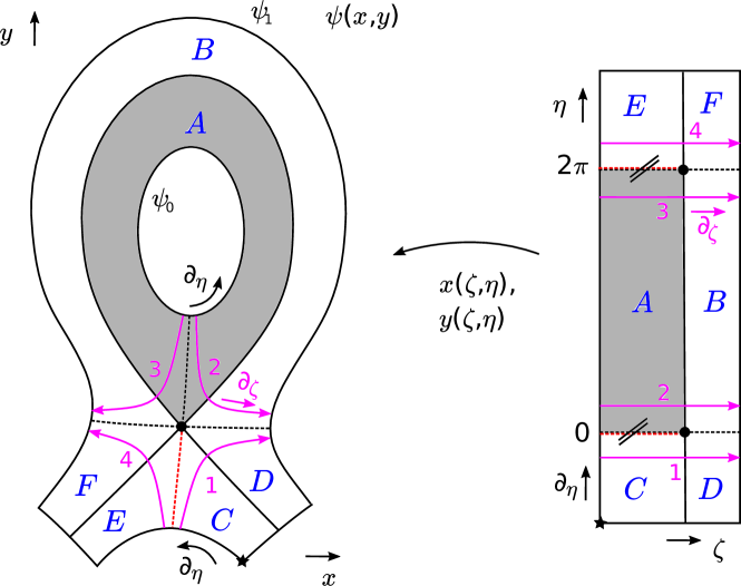
Figure 1: Sketch of coordinate transformation. The coordinates $x$ and $y$ (the physical space) are pulled back to the orthogonal coordinates $\zeta$, $\eta$ (computational space). Note the special topology of the 6 coordinate patches induced by the X-point. Patch A is periodic in $\eta$, which is depicted by the “double lines”. Patches C and E are connected, which we depict with the red dashed line.

Here, we show a sketch of the coordinate transformation. To the left we depict the physical space and to the right the computational space. The physical space is covered by 6 coordinate patches labelled A to F. The topology can be understood by following the neighbouring coordinate lines 1 and 4 as well as 2 and 3. When passing the separatrix, line 1 becomes adjacent to line 2, while line 3 changes neighbour to line 4. Also note that patch A is periodic and that patches C and E are connected. This type of structured grid, in which the topology between blocks has to be separately given, is called block-structured [25]. When implementing derivatives on the computational grid this topology has to be taken into account.

3.3 Normalization

Now, the problem is how and at what points to fix initial conditions for $a$ in order to integrate Eq. (9). We require that $a(x,y)$ is continuous and differentiable. One suggestion would be to set $a=a_{0}$ on an arbitrary contour line $\psi(x,y)=\psi_{0}$. This is indeed a valid choice for the case without X-point. However, as discussed above, the X-point exchanges the neighbours of streamlines that pass by it. This means that even though $a$ is continuous on neighbouring streamlines of $\partial/\partial\zeta$ initially, it is not guaranteed to be at later stages. Imagine we chose $a=const$ on the inner flux surface in Fig. 1. When we integrate Eq. (9) along $\partial/\partial\zeta$ beyond the separatrix some streamlines like number $2$ and $3$ change neighbours. This potentially induces discontinuities among the coordinate patches. Another uncertainty is the value of $a$ at the X-point itself since we approach the X-point from two different sides (line $1$ and $2$ for example). Similar issues appear if $a$ is chosen on a flux surface on the outside of the domain. Our solution to this problem is to initialize $a$ on the separatrix itself. Following streamlines along $\partial/\partial\zeta$ away from the separatrix neighbouring streamlines stay neighbours. Thus, if $a$ is continuous on the separatrix, the discontinuities among coordinate patches can be avoided.

We trace the separatrix with the streamline of $\frac{\partial}{\partial\eta}$ at $\zeta=0$. It can be parameterized by any suitable function. For the sake of discussion, let us choose the geometric angle $\theta$ defined with respect to an arbitrary point inside the innermost flux surface (cf. Reference [15]).

$$\left.\frac{\mathrm{d}x}{\mathrm{d}\theta}\right|_{\zeta=0}=\frac{x_{\eta}}{\theta_{\eta}} =\frac{-\psi_{y}}{\psi_{x}\theta_{y}-\psi_{y}\theta_{x}}$$ (10a)

$$\left.\frac{\mathrm{d}y}{\mathrm{d}\theta}\right|_{\zeta=0}=\frac{y_{\eta}}{\theta_{\eta}} =\frac{\psi_{x}}{\psi_{x}\theta_{y}-\psi_{y}\theta_{x}}$$ (10b)

$$\left.\frac{\mathrm{d}\eta}{\mathrm{d}\theta}\right|_{\zeta=0}=\frac{1}{\theta_{\eta}} =\frac{\sqrt{g}(\nabla\psi)^{2}}{\psi_{x}\theta_{y}-\psi_{y}\theta_{x}}a_{0}$$ (10c)

We normalize $a_{0}$ such that $\eta\in[0,2\pi]$ when we follow the separatrix in patch A in Fig. 1, that is,

$$2\pi=\oint_{\psi=0}\mathrm{d}\eta=\oint_{0}^{2\pi}\frac{\mathrm{d}\eta}{\mathrm{d}\theta}\bigg{|}_{\zeta=0}\mathrm{d}\theta$$

or

$$f_{0}=a_{0}=\frac{2\pi}{\int_{0}^{2\pi}\mathrm{d}\theta\frac{\sqrt{g}(\nabla\psi)^{2}}{\psi_{x}\theta_{y}-\psi_{y}\theta_{x}}}.$$ (11)

As initial point for the integration of Eq. (10) we can use any point with $\psi(x,y)=0$. These can be found with a standard bisection algorithm. Note that we cannot numerically integrate Eq. (10) across the X-point due to the vanishing gradient in $\psi$. However, we can integrate towards and close to the X-point. This might be numerically expensive since very small step sizes have to be used, but can be achieved with sufficient accuracy.

Having chosen values for $f_{0}$ and $a_{0}$ the coordinate transformation is now completely fixed. In order to find any coordinate $x(\zeta,\eta),y(\zeta,\eta)$ together with its Jacobian we integrate the streamlines of $\partial/\partial\eta$ and $\partial/\partial\zeta$ given in Eq. (7). We do this by first integrating $\partial/\partial\eta$ on the separatrix (where $a_{0}$ is known) up to the desired $\eta$ and then following $\partial/\partial\zeta$ up to $\zeta$ with the obtained starting point. In order to get $a$ we simply integrate Eq. (9) along the coordinate lines.

$$\left.\frac{\mathrm{d}x}{\mathrm{d}\zeta}\right|_{\eta=\text{const}} =\frac{\psi^{x}}{f_{0}(\nabla\psi)^{2}}$$ (12a)

$$\left.\frac{\mathrm{d}y}{\mathrm{d}\zeta}\right|_{\eta=\text{const}} =\frac{\psi^{y}}{f_{0}(\nabla\psi)^{2}}$$ (12b)

$$\left.\frac{\mathrm{d}a}{\mathrm{d}\zeta}\right|_{\eta=\text{const}} =-\frac{\Delta\psi}{f_{0}(\nabla\psi)^{2}}a$$ (12c)

First, however, we need to discuss how the computational domain should be discretized.

3.4 Discretization of the computational domain

As mentioned in the introduction and visible in Fig. 1 the computational domain is a product space. In order to keep this property also numerically we discretize the $\zeta$ and $\eta$ coordinates separately, i.e. we construct $N_{\zeta}$ equidistant cells in $\zeta$ and $N_{\eta}$ equidistant in $\eta$. Now, in order to maintain an integer number of equidistant cells in every block we impose certain restrictions. Let us define $L^{\text{in}}_{\zeta}=|f_{0}\psi_{0}|$ as the length of blocks A, C and E in $\zeta$ and $L^{\text{out}}_{\zeta}=|f_{0}\psi_{1}|$ as the length of blocks B, D and F. With this we have $L_{\zeta}:=L^{\text{in}}_{\zeta}+L^{\text{out}}_{\zeta}$. Furthermore, we define $L_{\eta}^{\text{out}}$ as the length of patch C, D, E and F in $\eta$ and $L_{\eta}^{\text{in}}$ as the length of A and B in $\eta$. We have $L_{\eta}:=L_{\eta}^{\text{in}}+2L_{\eta}^{\text{out}}$ and now define

$$q_{\zeta}:=L^{\text{out}}_{\zeta}/L_{\zeta}\quad q_{\eta}:=L_{\eta}^{\text{out}}/L_{\eta}.$$ (13)

Now, in order to guarantee an integer number of cells in each block we require that $N_{\zeta}^{\text{in}}:=(1-q_{\zeta})N_{\zeta}$, $N_{\zeta}^{\text{out}}:=q_{\zeta}N_{\zeta}$, $N_{\eta}^{\text{in}}:=(1-2q_{\eta})N_{\eta}$, and $N_{\eta}^{\text{out}}:=q_{\eta}N_{\eta}$ are integer numbers. Note that $q_{\zeta}$ being rational is a restriction on $L_{\zeta}$ and thus on the choice of $\psi_{0}$ and $\psi_{1}$. Only one of the two can be chosen freely. Analogously, the condition in $\eta$ is fulfilled by a proper choice of the boundaries in $\eta$. Furthermore, with this procedure we, in particular, achieve that the X-point always appears as the corner of a cell and never lies inside a grid cell.

3.5 Grid refinement

For the purposes of this study we use a very basic grid refinement technique. The idea is to simply divide each of $m_{\zeta}$ cells in the $\zeta$ coordinate on each side of the separatrix by $d_{\zeta}$ equidistant small cells and analogously in $\eta$ we divide each of $m_{\eta}$ cells next to the X-point by $d_{\eta}$. This means that in total we then have

$$N_{\zeta}^{\text{ref}}=N_{\zeta}+2m_{\zeta}(d_{\zeta}-1),\quad N_{\eta}^{\text{ref}}=N_{\eta}+4m_{\eta}(d_{\eta}-1)$$ (14)

cells in the $\zeta$ and $\eta$ directions. The factor $2$ in $\zeta$ appears because we refine the cells left and right of the separatrix each. In $\eta$ we have to consider that the X-point appears twice (cf. Fig. 1). Note that if we were to divide all cells in $\zeta$ by a factor $d_{\zeta}$, the refined grid would consist of $N_{\zeta}^{\text{ref}}=d_{\zeta}N_{\zeta}$ cells. In particular, this means that if the error of a numerical scheme is dominated by the refined patch, then the refined grid is equivalent to an unrefined grid with $d_{\zeta}N_{\zeta}$ grid points (analogous in $\eta$). The product space property is preserved in order to keep the implementation effort to a minimum.

3.6 Algorithm

Let us finally summarize the grid generation in the following algorithm. We assume that $\psi_{0}$ is given and we choose rational numbers $q_{\zeta}$ and $q_{\eta}$ such that $\psi_{1}=-q_{\zeta}\psi_{0}/(1-q_{\zeta})$, $\eta_{0}=-2\pi q_{\eta}/(1-2q_{\eta})$ and $\eta_{1}=2\pi(1+q_{\eta}/(1-2q_{\eta}))$. Furthermore, we assume that the $\zeta$ coordinate is discretized by a list of $N_{\zeta}$ values $\zeta_{i}$ with $i=0,1,\dots N_{\zeta}-1$ and $\eta$ is discretized by a list of $N_{\eta}$ values $\eta_{j}$ with $j=0,1,\dots N_{\eta}-1$. $N_{\zeta}$ and $N_{\eta}$ are chosen such that $q_{\zeta}N_{\zeta}$ and $q_{\eta}N_{\eta}$ are integer numbers. Finally the list of $\zeta_{i}$ and $\eta_{i}$ can be extended by the refinement points as described in Section 3.5.

1. Find the X-point. The X-point is often known or can be computed algebraically. Numerically, the zeroes of $\nabla\psi$ can be found very efficiently with a few Newton iterations, especially since the Hessian matrix of $\psi$ and its inverse are given analytically.

2. Find an arbitrary point $(x,y)$ with $\psi(x,y)=0$ and a suitable parameterization of Eq. (10) around the X-point.

3. Integrate Eq. (10) with $a_{0}=1$ over $\Theta=[0,2\pi]$ in patch A and use Eq. (11) to compute $f\equiv f_{0}$ and $a_{0}=a(\psi_{0})$. Use any convenient method for the integration of ordinary differential equations.

4. Integrate the streamline of Eq. (7b) with $\psi=0$ and $a=f_{0}$ from $\eta=0\dots\eta_{j}$ for all $j$. The result is a list of coordinates $x(0,\eta_{j}),y(0,\eta_{j})$ on the separatrix. These are divided into $N_{\eta}^{\text{in}}$ coordinates in patch A, and $N_{\eta}^{\text{out}}$ coordinates in patches C and E each.

5. Using this list and $a=f_{0}$ as starting values integrate Eq. (12) from $\zeta=0\dots\zeta_{i}$ for all $i$ and all $\eta_{j}$. This gives the map $x(\zeta_{i},\eta_{j}),y(\zeta_{i},\eta_{j})$ as well as $a(\zeta_{i},\eta_{j})$ for all $i$ and $j$.

6. Last, using these results and Eq. (6) evaluate the derivatives $\zeta_{x}(\zeta_{i},\eta_{j})$, $\zeta_{y}(\zeta_{i},\eta_{j})$, $\eta_{x}(\zeta_{i},\eta_{j})$, and $\eta_{y}(\zeta_{i},\eta_{j})$ for all $i$ and $j$.

4 The monitor metric approach for $\Delta\psi\neq 0$ at the X-point

For the following it is important to note that the theorems in Section 2 do not explicitly forbid the existence of a grid in the case $\Delta\psi\neq 0$, only the existence of an orthogonal grid. The notion of orthogonality, however, and especially the value of $\Delta\psi$, depends on the given metric tensor $g$ (recall Eq. (5) at this point). So what if we were allowed to change the metric tensor $g$ such that $\Delta\psi$ would vanish at the X-point? For example, consider the canonical metric $g^{ij}=\delta^{ij}$ and $\psi_{xx}+\psi_{yy}\neq 0$. If we change the canonical metric to an orthogonal metric $g^{xx}:=-\psi_{yy}$, $g^{yy}:=\psi_{xx}$, we can easily show that $\Delta\psi=0$ at the X-point in this metric. In this case the consistency equation (4) allows the existence of an orthogonal grid. Indeed, our idea for the construction of a grid for the case $\Delta\psi\neq 0$ at the X-point begins with changing the given metric to a more suitable metric. Then we use the algorithm in Section 3.6 to generate an orthogonal grid in the changed metric. This procedure of allowing the metric to be variable instead of a fixed given entity is called the monitor metric approach [25, 15].

Of course, now the question arises what happens to the physical, Cartesian metric, which we denote $G$ in the following. So far we have only considered the situation with one metric tensor $g$, the monitor metric. The important step is to allow the existence of two metric tensors. The first one is the artificial monitor metric tensor $g$ and the second one is the physical metric tensor $G$.

If we allow two metric tensors in our domain, we have in fact two different notions of angles and distances. We can measure angles, distances and areas either in $g$ or in $G$. This in particular means that if two vectors are orthogonal in one metric they might not be in the other. This is why the monitor metric approach does not violate our results from Section 2, which are true for both $g$ and $G$. For example, even if we can construct an orthogonal grid in the monitor metric $g$, in which the Laplacian of $\psi$ vanishes, it is still non-orthogonal in the physical metric $G$, in which the Laplacian of $\psi$ does not vanish, and thus does not violate Theorem 3, which forbids the existence of an orthogonal grid for $\Delta\psi\neq 0$. Unfortunately, there is no way around Theorem 4 and both volume elements $\sqrt{\bar{g}}$ and $\sqrt{\bar{G}}$ will diverge at the X-point.

It is important to realize that the monitor metric $g$ is an independent tensor and has nothing to do with the physical metric $G$. In fact, we would not even need a monitor metric tensor. The formulas in Section 2 can be simplified by defining $\chi^{ij}:=\sqrt{g}g^{ij}$ and we could then speak of a monitor tensor $\chi$, which must be symmetric and positive definite. This approach would be slightly more general as it also allows for the inclusion of adaption functions (see Reference [15]). For this discussion, however, we keep the metric tensor formulation for the sake of accessibility.

Finally, note that we use the monitor metric $g$ only for the construction of our grid. The physical equations still use the physical metric tensor $G$, which therefore also has to be transformed to the new coordinates. This is possible because with the help of Eq (6) we numerically construct not only the grid points $x(\zeta,\eta)$ and $y(\zeta,\eta)$ but also the elements of the Jacobian matrix. With the Jacobian matrix it is of course possible to transform any tensor to the $\zeta,\eta$ coordinate system, in particular the metric tensor $G$.

4.1 A constant monitor metric

The task is the construction of a suitable monitor metric. We suggest the constant tensor

$$g^{\text{cte}}=\alpha^{-1/2}\left(\frac{{\mathbf{v}}_{+}{\mathbf{v}}_{+}^{\mathrm{T}}}{\lambda_{+}}-\frac{{\mathbf{v}}_{-}{\mathbf{v}}_{-}^{\mathrm{T}}}{\lambda_{-}}\right),$$ (15)

where ${\mathbf{v}}_{+}$ and ${\mathbf{v}}_{-}$ are the normalized Eigenvectors of the Hessian matrix of $\psi$ at the X-point. $\lambda_{+}$ and $\lambda_{-}$ are the corresponding Eigenvalues. Since at the X-point (saddle point) the Hessian matrix is indefinite we can choose $\lambda_{-}$ to be the negative and $\lambda_{+}$ to be the positive Eigenvalue. We choose $\alpha$ such that the determinant of $g^{\text{cte}}$ is unity. With this choice $g^{\text{cte}}$ is symmetric, positive definite and $\Delta\psi=0$ at the X-point. A symbolic calculation shows us the explicit expression

$$g^{\text{cte}} =\alpha^{-1/2}\begin{pmatrix}\psi_{yy}^{2}-\psi_{xx}\psi_{yy}+2\psi_{xy}^{2}&-(\psi_{xx}+\psi_{yy})\psi_{xy}\\ -(\psi_{xx}+\psi_{yy})\psi_{xy}&\psi_{xx}^{2}-\psi_{xx}\psi_{yy}+2\psi_{xy}^{2}\end{pmatrix},$$

$$\alpha =\left(\psi_{xy}^{2}-\psi_{xx}\psi_{yy}\right)\left(\left(\psi_{xx}-\psi_{yy}\right)^{2}+4\psi_{xy}^{2}\right),$$ (16)

where all derivatives of $\psi$ are evaluated at the X-point. Note that $g^{\text{cte}}$ reduces to the identity if $\psi_{xx}=-\psi_{yy}$.

4.2 The bump monitor metric

As mentioned above, the monitor tensor in Eq. (16) produces non-orthogonal grids. This could be an issue if orthogonality at the boundary is a requirement, e.g. for the implementation of von Neumann boundary conditions. In fact, we need the monitor metric to take effect only in the vicinity of the singularity. The remaining grid may stay orthogonal in the physical metric $G$. We therefore introduce the bump-function with amplitude $1$ and radius $\sigma$ centred on the X-point

$$\epsilon(x,y) =\begin{cases}e^{1+\left(\frac{(x-x_{X})^{2}}{\sigma^{2}}+\frac{(y-y_{X})^{2}}{\sigma^{2}}-1\right)^{-1}}&\text{ for }(x-x_{X})^{2}+(y-y_{X})^{2}<\sigma^{2}\\ 0&\text{ else}\end{cases}.$$ (17)

With Eq. (17) we introduce

$$g^{\text{bump}}(x,y)=\bm{1}+\epsilon(x,y)\left(g^{\text{cte}}-\bm{1}\right),$$ (18)

where $\bm{1}$ is the identity tensor.

5 Applications of the algorithm

In this section we want to test the suggested algorithm in Section 3.6. We first present a completely analytical scenario and then proceed by solving elliptic equations for a more realistic test case. Please find codes and implementation details in the latest Feltor release [26]. Specifically, we generated the results in Sections 5.2-5.4 with the programs separatrix_orthogonal_t.cu, conformalX_elliptic_b.cu, geometryX_refined_elliptic_b.cu as well as geometry_diag.cu residing in the subdirectory feltor/inc/geometries/.

5.1 A simple example

It is instructive to analyse how the algorithm behaves in an analytical example. To this end let us consider again the flux-function from Example 2

$$\psi=\frac{1}{2}\left(2x^{2}-y^{2}\right)$$

together with the canonical metric tensor. We directly have $\psi_{x}=2x,\ \psi_{y}=-y$ and $\Delta\psi=1\neq 0$ in the canonical metric. The monitor metric (16) for the present problem becomes

$$g=\begin{pmatrix}1/\sqrt{2}&0\\ 0&\sqrt{2}\end{pmatrix}.$$

In this monitor metric we have $\psi^{x}=\sqrt{2}x$ and $\psi^{y}=\sqrt{2}y$ and $\Delta\psi=0$. Equation (12), parameterized by $y$, is therefore solved by $a=1$ and $x(y)=\pm x_{0}^{2}/2y$, which are the contour lines of the “correct” $\eta=xy$ coordinate we discussed in Example 2. In Fig. 2a we show the resulting grid.

Now, it is interesting to discuss what goes wrong if no monitor metric is used in connection with a non-vanishing Laplacian. Without monitor, Eq. (12) parameterized by $y$ reads

$$\frac{\mathrm{d}x}{\mathrm{d}y}=-\frac{2x}{y},\quad\frac{\mathrm{d}y}{\mathrm{d}y}=1,\quad\frac{\mathrm{d}a}{\mathrm{d}y}=\frac{a}{y}.$$

As initial conditions for $x$ and $y$ we choose the separatrix given by $y_{0}=\pm\sqrt{2}x_{0}$. As proposed in the algorithm we choose $a_{0}=1=$ const on the separatrix. We then have the solutions $a(y)=y/y_{0}$ and $x(y)=\pm y_{0}^{3}/(y^{2}\sqrt{2})$, which we plot in Fig. 2b and which lead to

$$a(x,y)=\left(\frac{|y|}{\sqrt{2}|x|}\right)^{1/3}.$$

This form of $a(x,y)$ is clearly problematic since then $\bar{G}_{\eta\eta}=1/(a^{2}(\nabla\psi)^{2})$ and the volume form $\sqrt{\bar{G}}=1/(a(\nabla\psi)^{2})$ diverge on the $y=0$ line and become $0$ for $x=0$. Note that $\bar{G}_{\eta\eta}$ determines the physical cell-size (length) $l_{\eta}=\sqrt{\bar{G}_{\eta\eta}}\triangle\eta$, where $\triangle\eta$ is the cell-size in the computational domain. If $\bar{G}_{\eta\eta}$ becomes very small, then so will $l_{\eta}$. This is clearly visible in Fig. 2b on the $x=0$ line. Now, a large variation in grid-size in a small region of the physical domain is highly undesirable in any numerical scheme. In advection type systems a small cell-size deteriorates the CFL condition, while in inversion problems the large variations in cell-size makes the discretization matrix highly ill-conditioned. On the other hand, large cell-sizes $\l_{\eta}$ at $y=0$ mean that this region cannot be accurately resolved. The cell-sizes seem unproblematic in Fig. 2b at $y=0$. However, the problem manifests in convergence studies, where the cell-size $\triangle\eta$ in the computational domain tends to zero. Since $l_{\eta}=\sqrt{\bar{G}_{\eta\eta}}\triangle\eta$ and $\bar{G}_{\eta\eta}\to\infty$ at $y=0$, the physical cell size $l_{\eta}$ might not tend to zero or not at the same rate as $\triangle\eta$. This behaviour deteriorates or completely inhibits convergence of a numerical scheme. We therefore conclude that using the algorithm without a proper monitor metric is inadvisable.

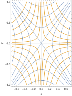
(a) with monitor (non-orthogonal)

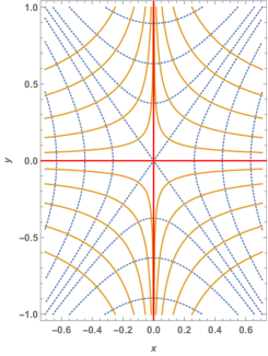
(b) without monitor (orthogonal)

Figure 2: Grids constructed for $\psi=(2x^{2}-y^{2})/2$ with (a) and without (b) monitor metric. We plot the contours $\psi\in\pm\{0,0.07,0.2,0.4\}$ in dotted blue; in solid orange we have the $\eta$ coordinates through the separatrix $y_{0}=\pm\sqrt{2}x_{0}$ with the points $x_{0}\in\pm\{0.1,0.2,0.3,0.4,0.5\}$. Without monitor metric the physical metric element $\bar{G}_{\eta\eta}$ becomes $0$ on the $x=0$ line and diverges on the $y=0$ line. We indicate this inconsistency with the solid red lines in (b).

5.2 Tokamak grids

Before we can construct a grid for a realistic scenario we need to construct an analytical flux-function with X-point. Reference [27] presents “One size fits all” analytic solutions to the Grad-Shafranov equation using Solov’ev profiles. The solution $\psi$ depends on thirteen coefficients. The exact values reside in the file geometry_params_Xpoint.js in feltor/inc/geometries of the accompanying dataset [26]. We will use this solution for $\psi$ throughout the remainder of this section.

In Fig. 3 we show the grid produced by our algorithm with and without refinement.

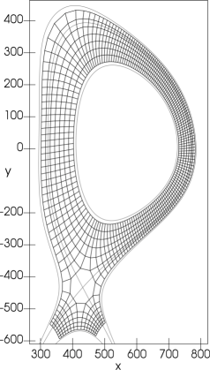
(a) regular grid

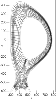
(b) refined grid

Figure 3: Orthogonal grids (in the monitor metric Eq. (18)) with $P=1$, $N_{\zeta}=8$ and $N_{\eta}=176$. We have $q_{\zeta}=1/4$ and $q_{\eta}=1/22$. Regular grid (a), and refined grid with $m_{\zeta}=m_{\eta}=1$ and $d_{\zeta}=d_{\eta}=4$ (b). Note that the nodes represent cell centres and not the actual cell boundaries. The grey lines denote the domain boundaries at $\psi_{0}=-15$ and $\psi_{1}=5$. We also plot the line $\psi=0$ to visualize the separatrix. Note the non-orthogonality at the X-point.

In the regular grid Fig. 3a the cell distribution is fairly homogeneous except in the vicinity of $x=y=350$, where cells become very large on the outside of the domain, and around the X-point. In the unrefined grid Fig. 3a the cells adjacent to the X-point are too large to sufficiently resolve this area. The resolution is improved in the refined version of the grid in Fig. 3b. Here, we divide the last cell on each side of the X-point in both the $\zeta$ and the $\eta$ direction by four (i.e. $m_{\zeta}=m_{\eta}=1$ and $d_{\zeta}=d_{\eta}=4$).

The here proposed refinement strategy is sufficient for the present study. However, in any production code the refinement techniques should be re-evaluated. The downside of the chosen product space refinement is that cells become unnecessarily small in the regions outside the X-point region. This is unfavourable for advection type equations. The goal must be to keep the cell sizes as homogeneous as possible across the domain so as not to deteriorate the CFL condition for advection-diffusion type problems. Fortunately, the X-point is a single point such that the refinement is local and shouldn’t present any performance issues. A direct solution could be giving up the product space property of the computational space and restricting the refinement to the area around the X-point. This, however, increases the implementation complexity. Let us point out here that there are advanced techniques available that might be worth considering for an efficient implementation. For elliptic grids it is known that with the help of adaption functions and monitor metrics the distribution of cells across the domain can be controlled. In this way the coordinate transformation itself includes a grid refinement [25, 28, 15, 29]. Although these techniques are very powerful their applicability to the present case remains to be explored. The difficulty lies in the fact that an elliptic equation has to be inverted on the domain, which can prove difficult to achieve due to the diverging metric at the X-point. A converging solver, however, is a prerequisite for the generation of elliptic grids. This motivates the following study.

5.3 Discretization of an elliptic equation

The two-dimensional elliptic equation $\Delta\phi=\rho$ in the new coordinates reads

$$\frac{\partial}{\partial\zeta}\left(\sqrt{\bar{G}}\left(\bar{G}^{\zeta\zeta}\frac{\partial\phi}{\partial\zeta}+\bar{G}^{\zeta\eta}\frac{\partial\phi}{\partial\eta}\right)\right)+\frac{\partial}{\partial\eta}\left(\sqrt{\bar{G}}\left(\bar{G}^{\eta\zeta}\frac{\partial\phi}{\partial\zeta}+\bar{G}^{\eta\eta}\frac{\partial\phi}{\partial\eta}\right)\right) =\sqrt{\bar{G}}\rho,$$ (19)

where we multiplied with the volume element to make the left hand side symmetric. In this equation $\bar{G}$ denotes the Cartesian metric $G$ transformed to the new coordinate system. We use this equation to test the quality of our grids.

We use a local discontinuous Galerkin method to discretize this equation on the computational ($\zeta,\eta$) domain [22]. This method approximates the solution by a order $P-1$ polynomial in each cell with $P$ being the number of polynomial coefficients. In contrast to finite element methods the approximation is allowed to be discontinuous at cell boundaries. As described in Reference [21] we compute the left side of Eq. (19) by discretizing the first derivatives $\partial/\partial\zeta$ and $\partial/\partial\eta$ with a forward discretization. These are just the discretizations we would have for the discretization of first derivatives in a Cartesian grid. Of course, we need to take into account the special topology of the computational space (cf. Fig. 1). Note that the derivative is a topological entity, which means that no metric is needed to define a directional derivative on a manifold [23]. The metric elements can be multiplied to the first derivatives by simple point-by-point multiplication. The second derivatives can be computed by using the adjoint of the first derivatives. Note that in the local discontinuous Galerkin scheme we need to add jump terms to the discretizations to penalize the discontinuities at the cell boundaries [22]. Without these the numerical solutions fail to converge at all. We are then finally left with a self-adjoint discretization of the elliptic operator.

It is a priori unclear whether our numerical scheme can cope with the diverging metric elements at the X-point, even if the metric or any other function is never evaluated at the X-point itself. Note that the coordinate singularity is weak in the sense that the integration over the volume element yields the correct volume of the domain. We verified this numerically, that is we numerically evaluate the volume $\int\mathrm{d}\zeta\mathrm{d}\eta\sqrt{\bar{G}(\zeta,\eta)}$ using Gauss–Legendre integration in computational space. We find equivalent results to integrating $\int_{\Omega}\mathrm{d}x\mathrm{d}y$ directly (with $\Omega$ being the physical domain) in Cartesian coordinates using a simple quadrature rule. Thus, the weakly formulated discontinuous Galerkin scheme should be able to cope with the diverging metrics without any necessary adaptions.

5.4 Convergence tests

We now test the convergence with a “bump” solution

$$\phi(x,y) =\begin{cases}e^{1+\left(\frac{(x-x_{0})^{2}}{\sigma^{2}}+\frac{(y-y_{0})^{2}}{\sigma^{2}}-1\right)^{-1}}&\text{ for }(x-x_{0})^{2}+(y-y_{0})^{2}<\sigma^{2}\\ 0&\text{ else}\end{cases}$$ (20)

with centre $(x_{0},y_{0})=(480,-300)$ and radius $\sigma=70$. This solution has no variation across the X-point situated at approximately $(x_{X},y_{X})=(431,-433)$. The boundary conditions are homogeneous Dirichlet in $\zeta$ and $\eta$. We plot the analytic solution Eq. (20) for the given parameters in Fig. 4.

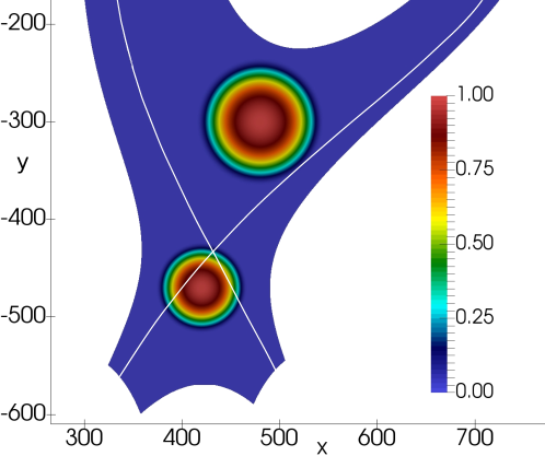
Figure 4: The location of our two “bump” solutions, the upper located at $(x_{X},y_{X})=(431,-433)$ with $\sigma=70$ and the lower bump located near the X-point at $(x_{0},y_{0})=(420,-470)$ with $\sigma=50$. We also indicate the location of the separatrix with the white line.

We can insert Eq. (20) into Eq. (19) to compute the corresponding right hand side analytically. With this right hand side given we then compute a numerical solution $\phi_{\text{num}}$ to Eq. (19). The relative error and the order of convergence can be defined in the $L_{2}$ norm as

$$\varepsilon=\left(\frac{\int_{\zeta_{0}}^{\zeta_{1}}\mathrm{d}\zeta\int_{\eta_{0}}^{\eta_{1}}\mathrm{d}\eta\sqrt{\bar{G}}(\phi_{\text{num}}-\phi_{\text{ana}})^{2}}{\int_{\zeta_{0}}^{\zeta_{1}}\mathrm{d}\zeta\int_{\eta_{0}}^{\eta_{1}}\mathrm{d}\eta\sqrt{\bar{G}}\phi_{\text{ana}}^{2}}\right)^{1/2},\quad\mathcal{O}=\frac{\ln[\varepsilon(2N)/\varepsilon(N)]}{\ln(2)},$$ (21)

where $\sqrt{\bar{G}}\mathrm{d}\zeta\mathrm{d}\eta$ is the correct volume form in the $\zeta,\eta$ coordinate system. The order $\mathcal{O}$ is computed via two consecutive errors, between which the number of cells $N$ is doubled.

		P=1		P=2		P=3		P=4
$N_{\zeta}$	$N_{\eta}$	error	order	error	order	error	order	error	order
4	88	5.46E+00		5.71E-01		5.95E-01		1.81E-01
8	176	4.53E-01	3.59	4.37E-01	0.39	1.35E-01	2.14	3.01E-02	2.59
16	352	2.33E-01	0.96	4.68E-02	3.22	1.06E-02	3.68	2.08E-03	3.86
32	704	1.99E-02	3.55	6.28E-03	2.90	8.14E-04	3.70	1.59E-04	3.71
64	1408	8.63E-03	1.21	1.33E-03	2.24	9.66E-05	3.07	1.32E-05	3.60
128	2816	4.41E-03	0.97	3.34E-04	2.00	1.32E-05	2.87	1.70E-06	2.95

Table 1: Convergence table for the bump solution Eq. (20) away from the X-point for various polynomial orders. No grid refinement is used. Error and order are defined via Eq. (21). Average orders are: ($2.06$, $P=1$); ($2.15$, $P=2$); ($3.09$, $P=3$); ($3.34$, $P=4$).

In Table 1 we show the error and corresponding orders for various polynomial orders and grid resolutions. A ratio of $N_{\eta}/N_{\zeta}=20$ is chosen such that the aspect ratio of the resulting cells is approximately unity. We observe a rather irregular convergence for all values of $P$. We attribute this behaviour to the irregular shapes of the grid cells at the location of the bump comparing Fig. 4 to Fig. 3. Although in this example there is no variation of the solution at the X-point the grid cells nevertheless become larger in its vicinity. Also the aspect ratio of the cells in the upper half of the bump are different from the aspect ratio in the lower half. We compute an average order of convergence with the values at $N_{\zeta}=4$ and $N_{\zeta}=128$ in an attempt to smooth the variations. The expected order $P$ is then approximately recovered for $P=2$ and $P=3$. For $P=1$ the average order is approximately $2$, however, the orders of the two finest grids indicate that only the expected first order is recovered. For $P=4$ the computed average order is more than $20$% too small. On the other side the absolute errors in the $P=4$ grids are the smallest among all grids. Finally, note that we also observed this irregular convergence in a similar example in Reference [15], where no X-point was present in the domain.

Let us now turn our attention to the case when variations around the X-point appear in the solution. We use the bump defined in Eq. (20) with $(x_{0},y_{0})=(420,-470)$ and $\sigma=50$. This is the lower bump in Fig. 4.

		P=1		P=2		P=3		P=4
$N_{\zeta}$	$N_{\eta}$	error	order	error	order	error	order	error	order
4	88	1.65E+01		1.36E+00		7.63E-01		8.74E-01
8	176	2.71E+00	2.60	6.48E-01	1.07	7.32E-01	0.06	3.28E-01	1.42
16	352	3.74E-01	2.86	8.43E-01	-0.38	3.70E-01	0.98	1.48E-01	1.15
32	704	5.72E-01	-0.61	2.98E-01	1.50	8.55E-02	2.11	8.84E-02	0.74
64	1408	1.95E-01	1.55	6.25E-02	2.25	1.83E-02	2.22	2.95E-02	1.58
128	2816	5.36E-02	1.86	3.48E-02	0.85	4.14E-02	-1.18	4.89E-03	2.59

Table 2: Convergence table for the bump solution Eq. (20) on the X-point for various polynomial orders. No grid refinement is used. Error and order are defined via Eq. (21). Average orders are: ($1.65$, $P=1$); ($1.06$, $P=2$); ($0.84$, $P=3$); ($1.50$, $P=4$).

In Table 2 we show the results of the same experiment as in Table 1. Also in this case the convergence rates are highly irregular and even negative in some cases. Again, we compute the average orders, which this time lie between $0.86$ and $1.5$. From this we conclude that the X-point reduces the convergence rate to around order $1$ for all numbers of polynomial coefficients. Inspection of the error reveals that indeed the error is entirely dominated by the region around the X-point. We attribute the loss of convergence to the diverging metric elements. As seen in Fig 3 these lead to large cell sizes in $\zeta$ and $\eta$. If we define the cell size in the computational domain as $\Delta_{\zeta}:=L_{\zeta}/N_{\zeta}$ and $\Delta_{\eta}:=L_{\eta}/N_{\eta}$, we compute the cell sizes in the physical domain by

$$l_{\zeta} :=\sqrt{\bar{G}_{\zeta\zeta}}\triangle\zeta=\sqrt{\bar{G}}\sqrt{\bar{G}^{\eta\eta}}\triangle\zeta\propto\sqrt{\bar{g}}\sqrt{\bar{g}^{\eta\eta}}\triangle\zeta=\left(a_{0}|\nabla\psi|\right)^{-1}\triangle\zeta,$$ (22a)

$$l_{\eta} :=\sqrt{\bar{G}_{\eta\eta}}\triangle\eta=\sqrt{\bar{G}}\sqrt{\bar{G}^{\zeta\zeta}}\triangle\eta\propto\sqrt{\bar{g}}\sqrt{\bar{g}^{\zeta\zeta}}\triangle\eta=\left(f_{0}|\nabla\psi|\right)^{-1}\triangle\eta,$$ (22b)

where we approximate the length in the actual Cartesian metric $G$ with the length in the monitor metric $g$. Clearly, the cell sizes $l_{\zeta}$ and $l_{\eta}$ diverge at the X-point due to the vanishing gradient in $\psi$. Now in the previous tests we looked for convergence in terms of $\triangle\zeta$ and $\triangle\eta$ that is $\varepsilon\propto\triangle\zeta^{P}$. However, it could be argued that the error should be proportional to $l_{\zeta}$ instead of $\triangle\zeta$. As long as $|\nabla\psi|$ is well-behaved the definitions are the same, but at the X-point this makes a difference. This means that even though we reduce $\triangle\zeta$ and $\triangle\eta$ in the computational domain, $l_{\zeta}$ and $l_{\eta}$ do not shrink with the same rate, which might explain the reduced orders in Table 2.

In order to remedy the loss of convergence due to large $l_{\zeta}$ and $l_{\eta}$ we use the grid refinement from Section 3.5. The grid refinement has the goal to reduce the sizes $\triangle\zeta$ and $\triangle\eta$ locally around the X-point until the physical lengths $l_{\zeta}$ and $l_{\eta}$ at the X-point equal the lengths in the remaining regions of the grid. If the error at the X-point is small enough, the error should then be dominated by the error in the remaining grid. Theoretically, this should then restore the expected order.

Numerically, we test this hypothesis using again the bump on the X-point as a solution to Eq. (19).

$N_{\zeta}\times N_{\eta}$	$4\times 88$		$8\times 176$		$16\times 352$		$32\times 704$
$d_{\zeta}=d_{\eta}$	error	order	error	order	error	order	error	order
1	7.63E-01		7.32E-01		3.70E-01		8.55E-02
2	7.32E-01	x	3.23E-01		9.54E-02		1.81E-02
4	3.70E-01		1.36E-01	2.43	2.19E-02	2.64	4.06E-02
8	8.54E-02		1.54E-01		5.28E-02		6.96E-03
16	1.79E-02		1.31E-01		1.41E-02		2.66E-03	3.04
32	5.38E-02		1.51E-01		1.68E-02		2.18E-03

Table 3: Convergence table for the bump solution Eq. (20) on the X-point for $P=3$ and increasing refinement. Note that for $N_{\zeta}\times N_{\eta}=4\times 88$ the bump lies entirely in the refined region. Error and order are defined via Eq. (21). The orders are computed with the error values in the same row the orders are indicated. For $N_{\zeta}\times N_{\eta}>4\times 88$ these are the rows where the error starts to stagnate with increasing refinement.

In Table 3 we show results for a fixed value $P=3$. We start with unrefined grids ($d_{\zeta}=d_{\eta}=1$) of increasing resolutions $N_{\zeta}$ and $N_{\eta}$. Then, we divide the last cells adjacent to the X-point into $d_{\zeta}=d_{\eta}$ parts and repeat the inversion of Eq. (19). Note that since we only refine the last cells adjacent to the X-point the actual region in the physical domain that is refined changes with grid resolutions. This leads to the effect that the solution for the lowest resolution lies entirely in the refined region and thus grid-refinement always leads to an improved error. In this case, the errors are equal to the corresponding $P=3$ column in Table 2, because, as discussed in Section 3.5, the refined grids are equivalent to the unrefined grids of increased resolution. Only for higher resolutions in $N_{\zeta}\times N_{\eta}$ we observe error stagnation for higher grid refinement. If we compute the order with the stagnating values, we recover $P\approx 3$.

In order to be entirely certain that the error is dominated by the unrefined region we repeat our experiment with the sum of both upper and lower bumps as a solution to Eq. (19) visible in Fig. 4.

$N_{\zeta}\times N_{\eta}$	$4\times 88$		$8\times 176$		$16\times 352$		$32\times 704$
$d_{\zeta}=d_{\eta}$	error	order	error	order	error	order	error	order
1	7.16E-01		4.57E-01		2.18E-01		4.96E-02
2	5.81E-01		1.92E-01		5.84E-02		1.06E-02
4	3.72E-01	x	1.21E-01	1.62	1.55E-02	2.97	2.35E-02
8	2.71E-01		1.33E-01		3.43E-02		4.19E-03
16	2.55E-01		1.18E-01		1.23E-02		1.66E-03	3.23
32	3.29E-01		1.33E-01		1.41E-02		1.43E-03

Table 4: Convergence table for the two bumps solution shown in Fig. 4 for $P=3$ and increasing refinement. Error and order are defined via Eq. (21). The orders are computed with the error values in the same row the orders are indicated. These are the rows where the error starts to stagnate with increasing refinement.

In Table 4 we show results for a fixed value $P=3$.

Now, the error first decreases and then stagnates even for $N_{\zeta}\times N_{\eta}=4\times 88$. The stagnating values are comparable to the stagnating values in Table 3 and the values in the $P=3$ column of Table 1. The latter observation strongly supports the conclusion that with enough refinement at the X-point the error is dominated by the error in the unrefined region. If we compute the order with the stagnating values, we indeed recover $P\approx 3$. The first value of $1.62$ at the $8\times 176$ could be explained by the relatively large errors in the $4\times 88$ and $8\times 176$ grids. Convergence only sets in at higher resolutions.

6 Conclusion

In summary we make two statements. First, a structured aligned orthogonal grid can be consistently constructed only when the separatrix forms a right angle ($\Delta\psi=0$) at the X-point. We discuss how with the help of a monitor metric the notion of orthogonality can change in a way that a grid construction is possible. This is based on our theoretical analysis and the following discussion of our algorithm for structured grid generation. Second, convergence of a numerical discretization of an elliptic equation on the grid may reduce to order one due to the diverging volume element or cell sizes at the X-point. Our local discontinuous Galerkin discretization converges with order approximately $P$ only as long as the solution is constant around the X-point. We show that grid refinement is needed around the X-point in order to achieve convergence at order greater than one, if the solution varies across the X-point. This is the typical situation in a practical application of the grid.

References

- [1] Wesson J 2011 Tokamaks 4th ed (Oxford University Press)
- [2] Rognlien T D, Milovich J L, Rensink M E and Porter G D 1992 J. Nucl. Mater. 196 347–351
- [3] Schneider R, Bonnin X, Borrass K, Coster D P, Kastelewicz H, Reiter A, Rozhansky V A and Braams B J 2006 Contrib. Plasma Phys. 46 3–191
- [4] Huysmans G T A and Czarny O 2007 Nucl. Fusion 47 659–666
- [5] Xu X Q, Umansky M V, Dudson B and Snyder R B 2008 Commun. Comput. Phys. 4 949–979
- [6] Chang C S, Ku S, Diamond P H, Lin Z, Parker S, Hahm T S and Samatova N 2009 Phys. Plasmas 16 056108
- [7] Hoelzl M, Gunter S, Wenninger R P, Muller W C, Huysmans G T A, Lackner K and Krebs I 2012 Phys. Plasmas 19 082505
- [8] Dudson B D, Allen A, Breyiannis G, Brugger E, Buchanan J, Easy L, Farley S, Joseph I, Kim M, McGann A D, Omotani J T, Umansky M V, Walkden N R, Xia T and Xu X Q 2015 J. Plasma Phys. 81 365810104
- [9] Tamain P, Bufferand H, Ciraolo G, Colin C, Galassi D, Ghendrih P, Schwander F and Serre E 2016 J. Comput. Phys. 321 606–623
- [10] Dudson B D and Leddy J 2017 Plasma Phys. Control. Fusion URL http://iopscience.iop.org/10.1088/1361-6587/aa63d2
- [11] Reiser D and Eich T 2017 Nucl. Fusion 57 046011 URL http://stacks.iop.org/0029-5515/57/i=4/a=046011
- [12] Galassi D, Tamain P, Bufferand H, Ciraolo G, Ghendrih P, Baudoin C, Colin C, Fedorczak N, Nace N and Serre E 2017 Nucl. Fusion 57 036029
- [13] Diamond P H, Itoh S I, Itoh K and Hahm T S 2005 Plasma Phys. Control. Fusion 47 R35–R161
- [14] D’haeseleer W, Hitchon W, Callen J and Shohet J 1991 Flux Coordinates and Magnetic Field Structure Springer Series in Computational Physics (Springer-Verlag)
- [15] Wiesenberger M, Held M and Einkemmer L 2017 J. Comput. Phys. 340 435–450
- [16] Nishimura Y and Lin Z 2006 Contrib. Plasma Phys. 46 551–556
- [17] Chang C S, Ku S, Diamond P, Adams M, Barreto R, Chen Y, Cummings J, D’Azevedo E, Dif-Pradalier G, Ethier S, Greengard L, Hahm T S, Hinton F, Keyes D, Klasky S, Lin Z, Lofstead J, Park G, Parker S, Podhorszki N, Schwan K, Shoshani A, Silver D, Wolf M, Worley P, Weitzner H, Yoon E and Zorin D 2009 J. Phys.: Conf. Ser. 180 012057
- [18] Zhang F, Hager R, Ku S H, Chang C S, Jardin S C, Ferraro N M, Seol E S, Yoon E and Shephard M S 2016 Eng. Comput. 32 285–293
- [19] Hariri F, Hill P, Ottaviani M and Sarazin Y 2014 Phys. Plasmas 21 082509
- [20] Stegmeir A, Coster D, Maj O and Lackner K 2014 Contrib. Plasma Phys. 54 549–554
- [21] Held M, Wiesenberger M and Stegmeir A 2016 Comput. Phys. Commun. 199 29–39
- [22] Cockburn B, Kanschat G, Perugia I and Schotzau D 2001 SIAM J. Numer. Anal. 39 264–285
- [23] Frankel T 2004 The geometry of physics: an introduction 2nd ed (Cambridge University Press)
- [24] Ribeiro T T and Scott B D 2010 IEEE Trans. Plasma Sci. 38 2159–2168
- [25] Liseikin V D 2007 A Computational Differential Geometry Approach to Grid Generation 2nd ed (Springer-Verlag)
- [26] Wiesenberger M and Held M 2018 Feltor v4.1 Zenodo URL http://doi.org/10.5281/zenodo.1207806
- [27] Cerfon A J and Freidberg J P 2010 Phys. Plasmas 17 032502
- [28] Glasser A H, Liseikin V D, Vaseva I A and Likhanova Y V 2006 Russ. J. Numer. Anal. Math. Modelling 21 481–505
- [29] Vaseva I A, Liseikin V D, Likhanova Y V and Morokov Y N 2009 Russ. J. Numer. Anal. Math. Modelling 24 65–78