Non-equilibrium turbulence scalings and self-similarity in turbulent planar jets

Abstract

We study the self-similarity and dissipation scalings of a turbulent planar jet and the theoretically implied mean flow scalings. Unlike turbulent wakes where such studies have already been carried out (Dairay et al., 2015; Obligado et al., 2016), this is a boundary-free turbulent shear flow where the local Reynolds number increases with distance from inlet. The Townsend-George theory revised by Dairay et al. (2015) is applied to turbulent planar jets. Only a few profiles need to be self-similar in this theory. The self-similarity of mean flow, turbulence dissipation, turbulent kinetic energy and Reynolds stress profiles is supported by our experimental results from 18 to at least 54 nozzle sizes, the furthermost location investigated in this work. Furthermore, the non-equilibrium dissipation scaling found in turbulent wakes, decaying grid-generated turbulence, various instances of periodic turbulence and turbulent boundary layers (Vassilicos, 2015, Dairay et al., 2015, Goto & Vassilicos, 2015, Nedic et al., 2017) is also observed in the present turbulent planar jet and in the turbulent planar jet of Antonia et al. (1980). Given these observations, the theory implies new mean flow and jet width scalings which are found to be consistent with our data and the data of Antonia et al. (1980). In particular, it implies a hitherto unknown entrainment behaviour: the ratio of characteristic cross-stream to centreline streamwise mean flow velocities decays as the -1/3 power of streamwise distance in the region where the non-equilibrium dissipation scaling holds.

1 Introduction

Industrial and environmental applications of turbulent free shear flows usually require knowledge of mean flow profiles. In the case of turbulent jets one most often needs to know how the mean flow velocity vector and the jet width evolve with downstream distance. The mean flow velocity vector has a cross-stream component which relates to entrainment. In the aforementioned applications entrainment is of paramount importance, for example in the effectiveness of heating/cooling by means of impinging jets (Carlomagno & Ianiro, 2014; Cafiero et al., 2017).

The modern theory of turbulent free shear flows has been initiated by Townsend (1976) and George (1989). It is based on hypotheses of self-similar profiles and the equilibrium dissipation scaling whereby the dissipation coefficient is constant. The dissipation coefficient $C_{\varepsilon}$ is defined as the ratio of the turbulence dissipation rate to the rate of non-linear energy losses by the largest turbulent eddies. This latter rate is proportional to the 3/2 power of the turbulent kinetic energy $K$ divided by a length-scale which characterizes the size of the largest turbulent eddies.

Self-similarity is usually justified in terms of loss of memory of inlet/initial conditions, which is why various previous investigations have sought to find self-similar profiles quite far downstream (Gutmark & Wygnanski, 1976; Kotsovinos & List, 1977; Kotsovinos, 1977; Everitt & Robins, 1978; Deo et al., 2008, 2013). However, the studies of axisymmetric turbulent wakes by Nedic et al. (2013), Dairay et al. (2015) and Obligado et al. (2016) found self-similar profiles starting from a downstream distance as close as ten times the wake generator size. Most industrial and even many environmental applications of turbulent wakes and jets are not concerned with the extremely far downstream flow. This makes the observation of self-similar profiles at closer distances particularly relevant and these distances amenable to theory.

Concerning the other hypothesis of the theory of Townsend (1976) and George (1989), the one about the turbulence dissipation scaling, Dairay et al. (2015) and Obligado et al. (2016) did not find support for a constant $C_{\varepsilon}$ in their experiments and numerical simulations of axisymmetric turbulent wakes even at distances of the order of 100 wake generator’s size. In fact, the turbulent planar jet investigations by Gutmark & Wygnanski (1976) and Antonia et al. (1980) did not find a constant turbulence dissipation coefficient either, even though their measurements extended up to streamwise distances as large as 160 nozzle widths. It may not have been fully clear at the time, but it is becoming increasingly clear now, that deviations from a constant $C_{\varepsilon}$ can imply deviations from current textbook scalings of wake/jet widths and centreline mean flow velocities. This is an important point which the present paper offers support for in the particular case of the turbulent planar jet.

Evidence of a new non-equilibrium scaling for $C_{\varepsilon}$ in flow regions where it is not constant has been found in turbulence generated by various different types of grids and in axisymmetric wakes (Vassilicos, 2015; Dairay et al., 2015), in both forced and freely decaying periodic turbulence (Goto & Vassilicos, 2015, 2016) and, most recently, in zero pressure gradient turbulent boundary layers (Nedic et al., 2017). This non-equilibrium dissipation scaling appears to have some universality as $C_{\varepsilon}$ is proportional to the ratio of a global Reynolds number to a local Reynolds number in all these cases. For example, in the axisymmetric turbulent wake case, the global Reynolds number $Re_{G}$ is defined in terms of wake generator size and incoming freestream velocity, and the local Reynolds number $Re_{\delta}$ is defined in terms of local wake width $\delta$ and the square root of the local centreline turbulent kinetic energy $K_{0}$. Explanations for the use of the word ”non-equilibrium” in this context can be found in Vassilicos (2015) and Goto & Vassilicos (2016).

Dairay et al. (2015) modified the theory of Townsend (1976) and George (1989) to take into account the non-equilibrium dissipation scaling and to also make the other assumptions of the theory more realistic and reduce them in number. They developed the theory for the case of the axisymmetric turbulent wake and deduced streamwise evolutions for the mean flow deficit and the wake width which differ from the well-known textbook scalings (Townsend, 1976; Tennekes & Lumley, 1972) yet fit experimental measurements well (Nedic et al., 2013; Dairay et al., 2015; Obligado et al., 2016).

In the present paper we start by describing the theory of turbulent planar jets with particular emphasis on the theory’s assumptions and predictions which we then confront with experimental data. To be assessed, the scaling predictions require data for the centreline mean flow velocity, the jet width and the centreline turbulence dissipation rate. To our knowledge the only previous study with sufficient and reliable experimental measurements of all these three quantities in a turbulent planar jet is the one by Antonia et al. (1980). We therefore use data from Antonia et al. (1980) and we also use data from the experimental study of Deo et al. (2008) which are also relatively rare in that they report streamwise profiles of both mean centreline velocity and turbulence dissipation rate in a turbulent planar jet. However, the data of Deo et al. (2008) that we use to study dissipation were obtained for an inlet/global Reynolds number that is six times smaller than that of Antonia et al. (1980) and this is reflected in the results of our analysis. We carry out our own experiment at an inlet Reynolds number that is about three times larger than that of Deo et al. (2008) with measurements that are extensive enough to allow for assessments of various self-similar profiles and various scalings, including the entrainment coefficient’s streamwise scaling which also turns out to be related to the turbulence dissipation scaling.

Previous turbulent shear flow experiments where the non-equilibrium dissipation scaling was observed were carried out in flows where the local Reynolds number decreases with downstream distance. In turbulent planar jets, the local Reynolds number $Re_{\delta}$ (defined on the basis of the local jet width $\delta(x)$ and the square root of the turbulent kinetic energy) increases with downstream distance $x$ from the nozzle exit. It is therefore particularly interesting to see whether the non-equilibrium dissipation scaling $C_{\varepsilon}\sim(Re_{G}/Re_{\delta})^{m}$ with $m=1$ for high enough Reynods number, and its consequences on the mean flow, also hold in a turbulent shear flow with such ”reversed” circumstances (Lumley, 1992; Castro, 2016). In the turbulent planar jet flow, $Re_{G}$ is defined on the basis of the inlet velocity $U_{J}$ and the size $h$ of the nozzle exit section (see figure 9a). As the paper shows, the theory also has some important implications for the jet entrainment coefficient as well as for the Reynolds shear stress scaling.

In section 2 we present the self-similarity theory of turbulent planar jets with particular attention to the assumptions and deductions of the theory. In section 3 we revisit the experimental turbulent planar jet data of Deo et al. (2008) and Antonia et al. (1980). In section 4 we describe our experimental apparatus and validate our data against previous measurements and in sections 5, 6 and 7 we report the results from our experimental tests of the following section’s assumptions and predictions. We conclude in section 8.

2 Mean field theory of turbulent planar jet flow

We apply to the turbulent planar jet flow the Townsend-George theory of incompressible turbulent free shear flow (see Townsend, 1976 and George, 1989) as revised by Dairay et al. (2015). This theory is based on the thin shear layer approximation of the Reynolds-averaged streamwise momentum balance

$$U\frac{\partial U}{\partial x}+V\frac{\partial U}{\partial y}=-\frac{\partial}{\partial y}R_{xy}$$ (1)

and on the continuity equation

$$\frac{\partial U}{\partial x}+\frac{\partial V}{\partial y}=0$$ (2)

where $U$ and $V$ are the mean flow velocities in the streamwise ($x$) and cross-stream ($y$) directions respectively (see Figure 9a) and $R_{xy}$ is the corresponding Reynolds shear stress (average of the product of streamwise and cross-stream fluctuating velocities obtained from a Reynolds decomposition involving the mean flow velocities $U$ and $V$ respectively). These two equations combined lead to re-writing the streamwise momentum balance as follows

$$\frac{\partial U^{2}}{\partial x}=-\frac{\partial}{\partial y}(VU+R_{xy}).$$ (3)

In all three versions of the Townsend-George theory (Townsend, 1976, George, 1989, Dairay et al., 2015) one starts by making the assumption that $U(x,y)$ is self-similar, i.e.

$$U(x,y)=u_{0}(x)f_{1}(y/\delta)$$ (4)

where $u_{0}(x)$ is the centreline and therefore maximum streamwise mean flow velocity at streamwise location $x$, and $\delta=\delta(x)$ is a measure of the jet width which we take to be

$$\delta(x)=\frac{1}{u_{0}(x)}\int_{0}^{\infty}\,U(x,y)\,\textup{d}y.$$ (5)

Integrating eq. (3) over $y$ across the jet and using the self-similar form of $U(x,y)$ (eq. 4) leads to

$$u_{0}^{2}(x)\delta(x)=U_{J}^{2}h.$$ (6)

The constancy of $u_{0}^{2}(x)\delta(x)$ (eq. (6)) in conjunction with the continuity (eq. (2)) of the planar mean flow, the self-similar form of $U(x,y)$ (eq. 4) and $V(x,0)=0$ imply that $V(x,y)$ is also self-similar, i.e.

$$V(x,y)=v_{0}(x)f_{2}(y/\delta),$$ (7)

and that $v_{0}$ and $u_{0}$ are related by

$$v_{0}=\alpha u_{0}\sim\frac{d\delta}{dx}u_{0}$$ (8)

where $\alpha\sim d\delta/dx$ is the entrainment coefficient (Pope, 2000).

Use of equation (3), the constancy of $u_{0}^{2}(x)\delta(x)$ (eq. (6)), the self-similar forms of both $U$ and $V$ (eqns. (4), (7)), and $R_{xy}(x,0)=0$ then imply that $R_{xy}$ is self-similar too, i.e.

$$R_{xy}(x,y)=R_{0}(x)g(y/\delta),$$ (9)

and that the $x$-dependence of $R_{0}$ is given by $R_{0}\sim u_{0}^{2}d\delta/dx$.

To close the problem and obtain explicit $x$-dependencies of $u_{0}$, $\delta$ and $v_{0}$, Townsend (1976) and George (1989) used the equation for the turbulent kinetic energy $K$,

$$U\frac{\partial K}{\partial x}+V\frac{\partial K}{\partial y}=P+T-\varepsilon$$ (10)

where $P$, $T$ and $\varepsilon$ stand for turbulence production, transport and dissipation respectively. At this point the approaches of Townsend (1976), George (1989) and Dairay et al. (2015) diverge in the detailed assumptions they make. A summary of the different assumptions is given in table 1. We follow Dairay et al. (2015) and assume self-similarity of $\varepsilon$, $K$ and $P+T$ and we write the first two terms as

$$K(x,y) = K_{0}(x)h(y/\delta)$$ (11)

$$\varepsilon(x,y) = D_{0}(x)e(y/\delta).$$ (12)

Use of eq. (10) leads to

$$\frac{K_{0}\,u_{0}}{\delta}\frac{d\delta}{dx}\sim D_{0},$$ (13)

a relation which was also obtained by Townsend (1976) and George (1989). This procedure adds the extra constraint eq. (13) and two further unknowns ($K_{0}$ and $D_{0}$) to our already four unknowns $u_{0}$, $v_{0}$, $\delta$ and $R_{0}$ and three constraints $R_{0}\sim u_{0}^{2}d\delta/dx$, $u_{0}^{2}\delta=U_{J}^{2}h$ and $v_{0}\sim u_{0}d\delta/dx$. We therefore have four constraints for six unknowns and, in general, we cannot proceed without two additional constraints to close the problem.

The one notable exception, as pointed out by Dairay et al. (2015), is when the non-equilibrium dissipation scaling can be invoked, namely $D_{0}=C_{\varepsilon}K_{0}^{3/2}/\delta\sim(Re_{G}/Re_{\delta})K_{0}^{3/2}/\delta$ where $Re_{\delta}=\sqrt{K_{0}}\delta/\nu$, in which case eq. (13) implies $u_{0}d\delta/dx\sim U_{J}h/\delta$ without interference from $K_{0}$. In this case the single additional hypothesis $D_{0}\sim(Re_{G}/Re_{\delta})K_{0}^{3/2}/\delta$ suffices to close the problem without further additional assumptions ($m=1$ case in table 1) and one obtains

$$u_{0}(x)/U_{J} = A\bigl{(}(x-x_{0})/h\bigr{)}^{-1/3}$$ (14)

$$\delta(x)/h = B\bigl{(}(x-x_{0})/h\bigr{)}^{2/3}$$ (15)

from $u_{0}d\delta/dx\sim U_{J}h/\delta$ and $u_{0}^{2}\delta=U_{J}^{2}h$ in terms of two dimensionless coefficients $A$ and $B$ and a unique virtual origin $x_{0}$. It follows that the entrainment coefficient $\alpha$ is not constant but depends on $x$ as $\alpha\sim d\delta/dx={2B\over 3}\bigl{(}(x-x_{0})/h\bigr{)}^{-1/3}$. This is a very different entrainment behaviour from the classical situation where $\alpha$ is independent of $x$.

To retrieve both the classical and more general scalings we follow Dairay et al. (2015) and consider the general dissipation scaling

$$D_{0}\sim(Re_{G}/Re_{\delta})^{m}K_{0}^{3/2}/\delta$$ (16)

where the special case $m=0$ corresponds to the classical equilibrium scaling used in the approaches of Townsend (1976) and George (1989). The theory is not conclusive without an additional assumption when $m\not=1$ so we adopt Townsend’s assumption that $K_{0}$ and $R_{0}$ have the same dependence on $x$, i.e. $K_{0}\sim R_{0}$ (Townsend, 1976). This makes the theory conclusive and leads to

$$u_{0}(x)/U_{J} = A\bigl{(}(x-x_{0})/h\bigr{)}^{-a}$$ (17)

$$\delta(x)/h = B\bigl{(}(x-x_{0})/h\bigr{)}^{2a}$$ (18)

$$2a = \frac{m+1}{2m+1}$$ (19)

which, in the classical equilibrium case $m=0$, leads to $2a=1$ and $\alpha$ independent of $x$ as predicted by Townsend (1976) and George (1989) and as reported in textbooks (e.g. Tennekes & Lumley, 1972, Davidson, 2004).

	Townsend (1976)		George (1989)		Dairay et al. (2015)
Self-similarity	$U,K,T,\varepsilon,u^{\prime},v^{\prime}$		$U,K,T,\varepsilon$		$U,K,P+T,\varepsilon$
Dissipation Scaling	$K_{0}^{3/2}/\delta$		$K_{0}^{3/2}/\delta$		$(Re_{G}/Re_{\delta})^{m}K_{0}^{3/2}/\delta$
Simplified production	no		$P\approx-R_{xy}dU/dy$		no
$R_{0}$	$\sim K_{0}$		no		no ($m=1$), $\sim K_{0}$ ($m\not=1$)

Table 1: Summary of the assumptions made in Townsend (1976), George (1989) and the present theory which has been adapted for planar jets from Dairay et al. (2015). The first row lists the quantities assumed to be self-similar. The second row gives the scaling assumed for the centreline turbulence dissipation rate. The third row states whether an approximation is or is not made for the production term. And the fourth row states if an assumption is or is not made concerning the centreline Reynolds shear stress. Notation: $u^{\prime}$ is the rms streamwise turbulent velocity and $v^{\prime}$ is the rms cross-stream (direction $y$) turbulent velocity.

The scalings obtained for three different values of $m$ are summarized in Table 2. The classical equilibrium scalings (Townsend (1976), George (1989)) correspond to $m=0$; the high Reynolds number non-equilibrium scalings correspond to $m=1$. It is worth pointing out that the entrainment coefficient $\alpha$ obeys

$$\alpha\sim 2aB\bigl{(}(x-x_{0})/h\bigr{)}^{2a-1}$$ (20)

and that it is constant only in the classical equilibrium case where $m=0$. We stress that the virtual origin $x_{0}$ is the same in equations (17), (18) and (20).

	Townsend (1976)-George (1989)	Present ($m=1$)
$u_{0}(x)$	$\sim(x-x_{0})^{-1/2}$	$\sim(x-x_{0})^{-1/3}$
$\delta(x)$	$\sim(x-x_{0})$	$\sim(x-x_{0})^{2/3}$
$\alpha\equiv v_{0}(x)/u_{0}(x)$	$\sim const$	$\sim(x-x_{0})^{-1/3}$

Table 2: Summary of the planar jet scalings obtained by Townsend (1976) and George (1989) and by the present version of the theory for $m=1$ (see eq. 16)). The present version of the theory leads to the same scalings as Townsend (1976) and George (1989) if $m=0$.

In the next section we revisit the experimental turbulent planar jet data of (Deo et al., 2008) and (Antonia et al., 1980) by paying particular attention to the fact that the virtual origin $x_{0}$ must be the same in all power-law dependencies on streamwise distance.

3 Centreline data from previous experiments

The turbulence dissipation scaling (eq. 16) is a pillar of the mean flow scaling eqns. (17), (18), (19) and (20). From eqns. (16), (17), (18) and (19),

$$D_{0}\sim(x-x_{0})^{-\gamma}$$ (21)

where the virtual origin $x_{0}$ must be the same as the one in eqns. (17) and (18) and

$$\gamma=\bigl{(}2a-\frac{1}{2}\bigr{)}m+\bigl{(}\frac{3}{2}+2a\bigr{)}.$$ (22)

Direct numerical simulations (DNS) of turbulent planar jets do not reach sufficiently high Reynolds numbers and very few laboratory studies report centreline turbulent dissipation profiles alongside centreline profiles of $u_{0}$ and/or $\delta$ for turbulent planar jets. The main exceptions seem to be the experimental data of Deo et al. (2008) who reported streamwise profiles of $D_{0}$ and $u_{0}$ (as well as some values of $\delta$ but at very few points, not enough for verifying eq. (18)) and the experimental data of Antonia et al. (1980) who reported streamwise profiles of $D_{0}$, $u_{0}$ and $\delta$ at an inlet/global Reynolds number $Re_{G}=42800$ which is about 6 times larger that the value of $Re_{G}$ in Deo et al. (2008). We now analyse these data by first identifying the single virtual origin which returns best fits to the streamwise scalings of the available quantities.

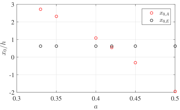
Figure 1: Virtual origins $x_{0,A}$ and $x_{0,E}$ obtained from the data of Deo et al. (2008) ($Re_{G}=7000$) by applying different exponents to the power laws eqns. (17) and (21) respectively, with $0.33\leq a\leq 0.5$ (i.e. $0\leq m\leq 1$ from eq. (19)). The optimal exponent $a=0.42$, corresponding to $m=0.2353$, is obtained for $x_{0}=x_{0,A}=x_{0,E}$.

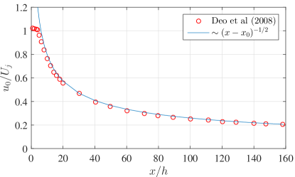
(a)

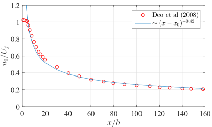
(b)

Figure 2: Normalised centreline streamwise mean velocity $u_{0}/U_{J}$ versus $x/h$. (a) Compared to eq. (17) with $a=0.5$ ($m=0$) and $x_{0}={x_{0,A}+x_{0,E}\over 2}\approx-0.65h$ (which differs from $x_{0,A}\approx 0.65h$ and $x_{0,E}\approx-1.95h$); (b) Compared to eq. (17) with $a=0.42$ ($m=0.2353$) and $x_{0}\approx 0.5h$ which is about the same as $x_{0,A}$ and $x_{0,E}$.

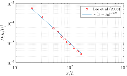
(a)

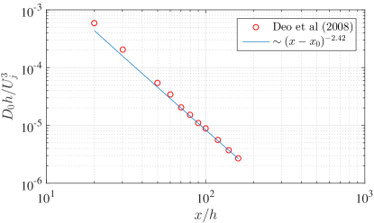
(b)

Figure 3: Centreline turbulence dissipation rate $D_{0}$ normalized with the inlet speed $U_{J}$ and the nozzle width $h$ versus $x/h$. (a) Compared to eq. (21) with $\gamma=5/2$ ($m=0$) and $x_{0}={x_{0,A}+x_{0,E}\over 2}\approx-0.65h$ which differs from $x_{0,A}\approx 0.65h$ and $x_{0,E}\approx-1.95h$; (b) Compared to eq. (21) with $\gamma=2.42$ ($m=0.2353$) and $x_{0}\approx 0.5h$ which is about the same as $x_{0,A}$ and $x_{0,E}$.

3.1 Deo et al. (2008)

A fundamental condition to be respected for the validity of the turbulent planar jet theory in section 2 is that the virtual origin used in equations (17)-(18)-(21) must be unique. In the case of Deo et al. (2008), we can only test the streamwise distance dependencies of eqns. (17) and (21), and this up to $x/h=160$ which is the location of their furthermost measurements. For values of $m$ ranging between $m=0$ and $m=1$ we set the corresponding exponents $a$ given by eq. (19) and find the virtual origin $x_{0,A}$ which returns the best fit of the data to eq. (17) in the range $10\leq x/h\leq 160$ (reasonable different choices of the lower bound of this range do not modify the results appreciably). In this way we obtain a value of $x_{0,A}$ for each $a$ which we plot in figure 1. We apply the same procedure to the dissipation data provided by Deo et al., 2008 and obtain different virtual origins $x_{0,E}$ which return a best fit to eq. (21) for different values of $\gamma$ corresponding to values of $m$ between $m=0$ and $m=1$. In figure 1 we plot $x_{0,E}$ versus $a$, given that $\gamma$ is a function of $a$ and $m$ via eq. (22) and that $a$ and $m$ are related by eq. (19). The virtual origin $x_{0}$ must be such that $x_{0}=x_{0,A}=x_{0,E}$ and the only exponent $a$ where this happens is $a=0.42$ which corresponds to $m=0.2353$ (see eq. (19)). These values of $a$ and $m$ are different from the classical ones, $a=0.5$ and $m=0$, but they are also different from the non-equilibrium exponents $a=1/3$ and $m=1$.

In figure 2(a) we plot $u_{0}/U_{J}$ versus $x/h$ with the classical fit $(x-x_{0})^{-0.5}$ and in figure 3(a) we plot $D_{0}h/U_{J}^{3}$ versus $x/h$ with the classical fit $(x-x_{0})^{-5/2}$ ($\gamma=5/2$ for $m=0$). We have chosen the same $x_{0}$ for these two fits, half way between $x_{0,A}\approx 0.65h$ and $x_{0,E}\approx-1.95h$ which are the values for $a=0.5$ in figure 1. We compare these fits with those in figures 2(b) and 3(b) where we plot the same data but fitted, respectively, with $(x-x_{0})^{-0.42}$ and $(x-x_{0})^{-2.42}$ where $x_{0}\approx x_{0,A}\approx x_{0,E}\approx 0.5h$, as this is the case where a single virtual origin does exist.

It may be argued that the fits in figures 2 and 3 are slightly better for the classical exponents $a=0.5$ and $\gamma=2.5$, but the fits with $a=0.42$ and $\gamma=2.42$ are not bad either and they are obtained with a consistently optimal virtual origin whereas those for $a=0.5$ and $\gamma=2.5$ are not. If the only theoretical option was $a=0.5$ and $\gamma=2.5$ one might have been able to conclude that the data of Deo et al. (2008) fit this option well and perhaps overlook the appreciable divergence between $x_{0,A}$ and $x_{0,E}$. However, now that there are more options available, it becomes more difficult to overlook this difference and conclude.

As already mentioned, the turbulence dissipation scaling eq. (16) is a key pillar underpinning eqns. (17)-(18)-(21). However, the data which would be necessary to directly test the validity of eq. (16) are not in Deo et al. (2008). Furthermore, Dairay et al. (2015) show that eq. (16) appears with $m\approx 1$ in axisymmetric turbulent wakes only when the Reynolds number is large enough. Obligado et al. (2016) also demonstrated that it is much more difficult to distinguish between different values of $m$ by fitting streamwise mean flow profile data than by directly fitting the dissipation scaling (eq. 16) in the case of axisymmetric turbulent wakes. It is therefore important to analyse turbulent planar jet data with inlet Reynolds numbers much higher than those of Deo et al. (2008) where $Re_{G}=7000$; and it is also important that these data are complete enough to permit checks of eqns. (17)-(18)-(16) and (21). Such data can be found in Antonia et al. (1980).

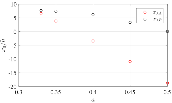
Figure 4: Virtual origins $x_{0,A}$ and $x_{0,B}$ obtained from the data of Antonia et al. (1980) ($Re_{G}=42800$) by applying different exponents to the power laws eq. (17) and eq. (18) respectively, with $0.33\leq a\leq 0.5$ (i.e. $0\leq m\leq 1$ from eq. (19)). The optimal exponent is the one where $x_{0}=x_{0,A}=x_{0,E}$, i.e. $a=1/3$ corresponding to $m=1$.

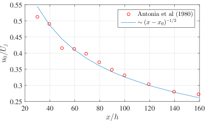
(a)

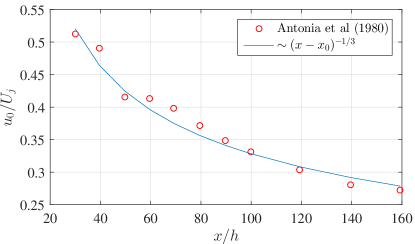
(b)

Figure 5: Normalised centreline streamwise mean flow velocity $u_{0}/U_{J}$ versus $x/h$. (a) Compared to eq. (17) with $a=1/2$ ($m=0$) and $x_{0}={x_{0,A}+x_{0,B}\over 2}\approx-9.4h$ which differs from $x_{0,A}\approx-19h$ and $x_{0,B}\approx 0$; (b) Compared to eq. (17) with $a=1/3$ ($m=1$) and $x_{0}\approx 7h$ which is about the same as $x_{0,A}$ and $x_{0,B}$.

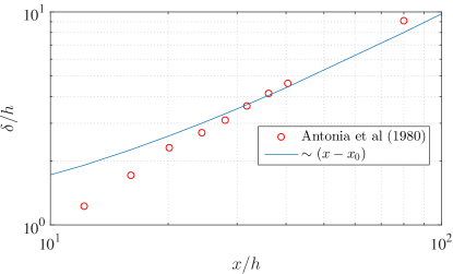
(a)

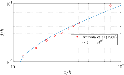
(b)

Figure 6: Normalised jet width $\delta/h$ versus $x/h$. (a) Compared to eq. (18) with $2a=1$ ($m=0$) and $x_{0}={x_{0,A}+x_{0,B}\over 2}\approx-9.4h$ which differs from both $x_{0,A}\approx-19h$ and $x_{0,B}\approx 0$; (b) Compared to eq. (18) with $2a=2/3$ ($m=1$) and $x_{0}\approx 7h$ which is about the same as $x_{0,A}$ and $x_{0,B}$.

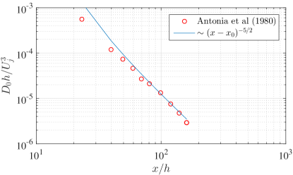
(a)

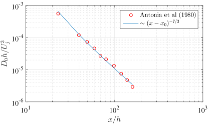
(b)

Figure 7: Centreline turbulence dissipation rate $D_{0}$ normalized with the inlet speed $U_{J}$ and the nozzle width $h$ versus $x/h$. (a) Compared to eq. (21) with $\gamma=5/2$ ($m=0$) and $x_{0}=-9.5h$; (b) Compared to eq. (21) with $\gamma=7/3$ ($m=1$) and $x_{0}\approx 7h$.

3.2 Antonia et al. (1980)

Antonia et al. (1980) report centreline data for $u_{0}$ in a turbulent planar jet with inlet/global Reynolds number $Re_{G}=42800$ from $x/h=30$ to $x/h=160$, and also data for $\delta$ from $x/h=12$ to $x/h=100$. In figure 4 we plot the virtual origins $x_{0,A}$ and $x_{0,B}$ which return the best respective fits of these data to eqns. (17) and (18) for values of $a$ ranging between $1/3$ ($m=1$) and $1/2$ ($m=0$). The only exponent $a$ where $x_{0,A}\approx x_{0,B}$ is $a\approx 1/3$. This is therefore the only exponent $a$ for which the data of Antonia et al. (1980) can fit both eqns. (17) and (18) in a way that respects the momentum flux conservation eq. (6).

It is noticeable that the optimal virtual origin $x_{0,B}$ varies much less with $a$ than $x_{0,A}$. This is because the exponent $a$ in the power law (eq. 17) is smaller than the exponent $2a$ in the power law (eq. 18). The exponent $\gamma$ in eq. (21) is even larger and varies between $5/2$ and $7/3$ in the range $0\leq m\leq 1$ where $a$ varies from $1/2$ to $1/3$. It is therefore no surprise that the virtual origin $x_{0,E}$ which optimises the fit of eq. (21) to the centreline dissipation data of Antonia et al. (1980) (ten data points from $x/h=20$ to $x/h=160$) turns out to be about the same for all values of $a$ between $1/3$ and $1/2$ and is in fact quite close to $x_{0,E}/h=5$ on average. The quality of this centreline dissipation fit does not vary significantly if $x_{0,E}/h$ is made to vary between 3 and 7 for any value of $a$ between $1/3$ and $1/2$. The virtual origin $x_{0}/h=7$ which optimises both power law fits (eqns. 17) and (18) in the case $a=1/3$ (i.e. $m=1$) is also effectively optimal for the fit of eq. (21) with $\gamma=7/3$ (i.e. $a=1/3$, $m=1$) to the centreline dissipation data of Antonia et al. (1980). No other exponent $a$, or equivalently $m$, can achieve an optimally good fit of the data of Antonia et al. (1980) to all three power laws (eqns. 17), (18) and (21) with one single virtual origin $x_{0}=x_{0,A}=x_{0,B}=x_{0,E}$.

In figures 5, 6 and 7 we plot streamwise profiles of $u_{0}/U_{J}$, $\delta/h$ and $D_{0}h/U_{J}^{3}$ respectively using the data of Antonia et al. (1980). The left plots show fits of these data to the classical power laws which correspond to $m=0$, all with the same virtual origin $x_{0}$ as must of course be the case. However, given the wide difference between $x_{0,A}$ and $x_{0,B}$ (see figure 4) for $m=0$, i.e. $a=0.5$, the single virtual origin $x_{0}$ in all figures 5(a), 6(a) and 7(a) has been chosen to be midway between $x_{0,A}$ and $x_{0,B}$. The fits in the right plots 5(b), 6(b) and 7(b) are to the non-equilibrium power laws which correspond to $m=1$. In this case the virtual origin is unambiguous and naturally the same for all the plots as this is the only case where the data of Antonia et al. (1980) are best fitted with one same virtual origin for all three quantities $u_{0}$, $\delta$ and $D_{0}$. The equilibrium ($m=0$) fit of $u_{0}$ is arguably a little better than the non-equilibrium fit ($m=1$) of $u_{0}$, but the non-equilibrium fits of $\delta(x)$ and $D_{0}(x)$ are both clearly superior to the equilibrium fits of these two quantities. All in all, the data of Antonia et al. (1980) seem to favour the non-equilibrium power-law dependencies on streamwise distance and we now use further data from their paper for a direct check of the non-equilibrium dissipation scaling which underpins the non-equilibrium fits in figures 5, 6 and 7.

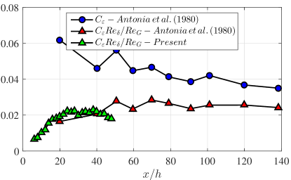
Figure 8: Centreline dissipation coefficient $C_{\varepsilon}\equiv 2D_{0}\delta/(3u^{\prime 3})$ (blue circles) and $C_{\varepsilon}\cdot Re_{\delta}/Re_{G}$ (red triangles), both from Antonia et al. (1980) where $Re_{G}=42800$ (red triangles)). The green triangles are $C_{\varepsilon}\cdot Re_{\delta}/Re_{G}$ from our present data ($Re_{G}=20000$, see section 4) where $C_{\varepsilon}$ is also calculated from $C_{\varepsilon}\equiv 2D_{0}\delta/(3u^{\prime 3})$ on the centreline. The quantities in this figure are plotted as functions of normalised streamwise distance $x/h$.

Antonia et al. (1980) also provided centreline streamwise profile data in the range $20\leq x/h\leq 140$ for the rms turbulent velocity $u^{\prime}$ normalised by $u_{0}$, i.e. $u^{\prime}/u_{0}$, and for $D_{0}\delta/u_{0}^{3}$. It is therefore possible to obtain, from their data, the turbulence dissipation coefficient $C_{\varepsilon}\equiv 2D_{0}\delta/(3u^{\prime 3})$ which we plot in figure 8 against $x/h$. This figure shows that $C_{\varepsilon}$ decreases with increasing $x/h$ in the range $20\leq x/h\leq 140$. However, $C_{\varepsilon}Re_{\delta}$ appears to remain constant in the range $40\leq x/h\leq 140$ (figure 8), which is consistent with the non-equilibrium exponent $m=1$ in eq. (16). The largest difference between two values of $C_{\varepsilon}Re_{\delta}$ in this range is 15% of the mean (over the same range) of $C_{\varepsilon}Re_{\delta}$ whereas it is 46% for $C_{\varepsilon}$. In the range $50\leq x/h\leq 140$ these percentages are even more convincing as they are 3.5% and 46% respectively. The data of Antonia et al. (1980) support $C_{\varepsilon}Re_{\delta}=Const$ (i.e. $m=1$) rather than $C_{\varepsilon}=Const$ (i.e. $m=0$) quite clearly in the range $50\leq x/h\leq 140$ and perhaps even $40\leq x/h\leq 140$.

There are of course two potential caveats in this conclusion both of which result from the fact that the measurements of Antonia et al. (1980) were taken with single hot wire anemometry. Strictly speaking, $C_{\varepsilon}$ should be defined as $C_{\varepsilon}\equiv D_{0}\delta/K_{0}^{3/2}$ rather than $C_{\varepsilon}\equiv 2D_{0}\delta/(3u^{\prime 3})$ and all fluctuating velocity gradients should be accessed for a measurement of $\varepsilon$ which does not rely on assumptions. Antonia et al. (1980) used the isotropic approximation of $\varepsilon$ which is accessible with single hot wire measurements and thereofre relied on the assumption of small-scale isotropy. These issues are addressed in the following section and in section 5.

In the following section we describe our turbulent planar jet experiment and validate it against previously published data. We take Hot Wire Anemometry (HWA) measurements with both single and cross wires and investigate the validity of the assumptions and predictions of the theory described in section 2. Our measurements do not extend beyond $x/h=54$, but we do measure and report in sections 5, 6 and 7 profiles of $U$, $V$, $R_{xy}$, $K$ and $\varepsilon$. Our global/inlet Reynolds number is $Re_{G}=20000$ and therefore nearly three times larger than $Re_{G}=7000$ in Deo et al. (2008). It is also about half the value of $Re_{G}$ in Antonia et al. (1980), and the factor 2 between our $Re_{G}=20000$ and the $Re_{G}=42800$ of Antonia et al. (1980) can help us assess the universal non-equilibrium expectation that the constant in $C_{\varepsilon}\cdot Re_{\delta}=Const$ is in fact proportional to $Re_{G}$, in full agreement with $m=1$.

4 Experimental apparatus and measurements

Our planar jet flow is generated using a centrifugal blower which collects air from the environment and then forces it into a plenum chamber. In order to reduce the inflow turbulence intensity level and remove any bias due to the feeding circuit, the air passes through two sets of flow straighteners before entering a convergent duct (having area ratio equal to about 8). At the end of the duct there is a letterbox slit with aspect ratio $s/h=31$ and $h=15mm$ (see Figure 9a). Figure 9a includes a schematic of the contoured inlet: in order to produce a top hat velocity profile at the jet exit ($x=0$), the two longest sides of the slit are filleted with a radius $r=2h$ (see Figure 9b), following the careful recommendation by Deo et al. (2007). The jet exhausts into ambient air and is confined in the spanwise direction by two perspex walls (see Figure 9b) of size $100h\times 100h$ placed in $x-y$ planes. The aspect ratio $s/h=31$ is sufficiently large to ensure that the flow can be considered planar as documented in the published literature (e.g. Gutmark & Wygnanski, 1976; Gardon & Akfirat, 1966). Furthermore, the effect of the boundary layer which develops on the bounding perspex walls is estimated to affect less than 3% of the overall spanwise extent $s$ at 100 $h$ from the jet exit section. The jet rig is located in a room much larger in all directions than the jet width $\delta$ at $x=100h$, so that the effects of the ceiling, floor and room walls on the entrainment and development of the jet flow are reduced to a minimum.

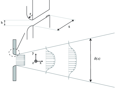
(a)

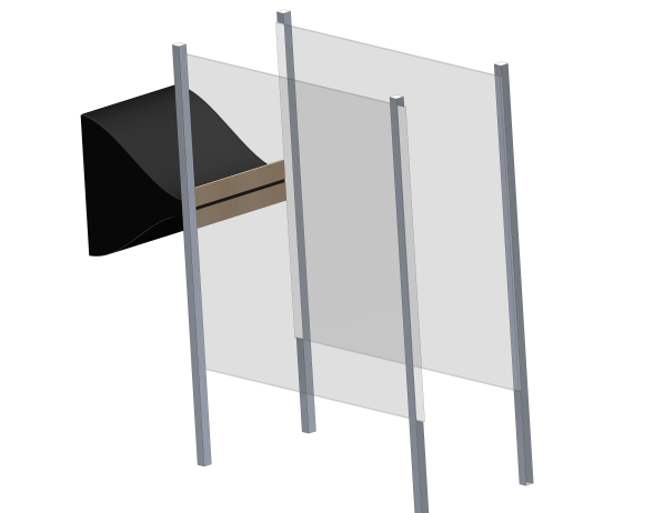
(b)

Figure 9: a) Schematic representation of the planar jet flow, with detail of the fillet radius $r$; $\delta(x)$ is representative of the jet width at each streamwise location $x$. b) Isometric representation of the experimental apparatus employed to generate the planar jet.

The inlet velocity $U_{J}=20m/s$ is set and stabilized using a PID feedback controller which takes as input the thermo-fluid-dynamic conditions of the flow measured by a thermocouple and a Pitot tube. The thermocouple measures the temperature of the working fluid about 5 $cm$ upstream of the letterbox slit in the convergent part of the nozzle, whilst the Pitot tube is located such that the pressure measurements are carried out within the potential core of the jet flow. These data are acquired using a Furness Control micromanometer FCO510, then manipulated by the in house PID controller which outputs the voltage to be supplied to the blower’s driver in order to achieve the desired flow speed.

The velocity signal is measured using both one- and two-component hot wires (herein referred to as SW and XW respectively) driven by a Dantec Streamline constant temperature anemometer (CTA). Considering the large dynamic range that characterizes the planar jet flow, we operate both the SW and the XW with an overheat ratio of 1.2. Both the SW and the XW are etched in house; the sensing length of the wire is $\approx$1 $mm$, whilst the wire diameter is $5\mu m$. For the XW, the separation between the two wires is about 1$mm$. Data are sampled at a frequency of 50 $KHz$ using a 16-bit National Instruments NI-6341 (USB) data acquisition card. Each SW measurement lasts for 60$s$, which was estimated to be a sufficiently long time for convergence of the turbulent statistics studied here. This was checked by taking longer time SW measurements, up to two minutes at the furthermost investigated location (i.e. $x/h=50$) where the integral length-scale is the largest and checking the convergence of the longitudinal integral length-scale $L_{uu}$. (The number of integral scales within a 60$s$ sampling period is about 30000 at $x/h=50$ and is of course higher at locations closer to the nozzle exit.) The acquisition time for XW measurements was increased to 120$s$ in all cases because they involve the cross-stream velocity which is of the order of 2-3% of the streamwise velocity.

Cross-stream profiles were acquired with the SW probe from $x/h=0$ to $x/h=50$ with a 2$h$ spacing. These measurements were taken for inlet Reynolds number $Re_{G}=U_{J}h/\nu=20000$. We ascertained that the jet is indeed planar by also taking measurements at $z=\pm 10h$ and verifying that there are no statistical differences between the three sampled values of $z$.

Cross-stream profiles were also taken with the XW probe in order to measure both the cross-stream mean velocity component($V$) and the relevant component $R_{xy}$ of the Reynolds stress tensor, for the same inlet Reynolds number. Cross-stream profiles were measured at 10 different streamwise locations ranging from 14$h$ to 54$h$. The probe displacement through the flow field is ensured by a high precision traverse system controlled by a in-house driving system. We verified that no significant differences exist between SW and XW measurements of same statistics.

The SW calibration is carried out at the beginning and end of each run and is obtained by fitting data acquired at seven different inlet speeds (ranging from 0 to 100% of $U_{J}$) with a 4-th order polynomial curve. For the XW, a similar procedure is applied with the additional introduction of 9 angles of the probe with respect to the streamwise direction (in the $x-y$ plane), ranging from -30^∘ to 30^∘. This range of angles was chosen on the basis of previous planar jet investigations, e.g. Browne et al. (1984), and by checks done with a wider range of angles (i.e. $\pm 35^{\circ}$). Experimental runs showing differences between calibrations at beginning and end of the run larger than 1% are discarded and repeated. Particular care was also taken with respect to temperature drift during runs: in all cases, there were no excursions larger than 0.3$K$ between start and end of run.

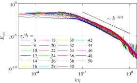
(a)

(b)

Figure 10: a) Streamwise fluctuating velocity spectra measured along the jet centreline using SW data plotted against the normalised longitudinal wavenumber $k\eta$. b) Cross-stream fluctuating velocity spectra measured along the jet centreline using XW data plotted against the normalised longitudinal wavenumber $k\delta$.

The velocity spectra $E_{uu}$ (of the streamwise fluctuating velocity) and $E_{vv}$ (of the cross-stream fluctuating velocity) provide information about large scale and small scale resolution of our measurements as well as presence of coherent/periodic structures. Figure 10a is a plot of $E_{uu}$ on the jet centreline region $6\leq x/h\leq 50$. Data are plotted against the longitudinal wavenumber on the basis of the Taylor hypothesis ($k=2\pi f/u_{0}$ where $f$ stands for frequency) multiplied by the Kolmogorov lengthscale $\eta\equiv(\nu^{3}/\varepsilon)^{1/4}$. The temporal resolution of the wire is not enough to resolve the dissipative scales immediately past the potential core. However, in the region of major interest for the present study, namely $x/h>18$ as established in the following sections, the small scales are resolved sufficiently well. The large scales are also well resolved given the small wavenumber plateau in Figure 10(a). As the streamwise distance increases, the increasing value of $E_{uu}$ at low wavenumbers is due to the increase of the longitudinal integral length-scale $L_{uu}$ given that $L_{uu}=E_{uu}(0)u_{0}/(4u^{\prime 2})$ (Tennekes & Lumley, 1972). Similar observations and comments can be made for the cross-stream spectrum $E_{vv}$.

We plot the lateral velocity spectra $E_{vv}$ calculated along the jet centreline against $k\delta$ rather than $k\eta$ in Figure 10b to bring out the fact that the peak in this spectrum scales with $\delta(x)$. A peak can clearly be spotted at $k\delta\approx 1$, corresponding to $f\delta/u_{0}\approx 0.16$ (in agreement with Deo et al., 2008), at all investigated centreline streamwise distances. These peaks must be associated with jet coherent structures.

The estimate of the turbulent dissipation rate $\varepsilon$ is obtained from its isotropic surrogate, i.e. $\varepsilon_{ISO}=15\nu\overline{(\partial u/\partial x)^{2}}$, by integrating the one dimensional spectrum $E_{uu}$ following

$$\overline{(\partial u/\partial x)^{2}}=\int_{0}^{\infty}k^{2}E_{uu}dk$$ (23)

where $u$ is the streamwise turbulent fluctuating velocity. We also follow Antonia et al. (1980) and chose to estimate $\varepsilon$ from $\varepsilon_{iso}$ rather than from XW data because of the better resolution of the SW data. This choice is supported by the DNS results of Stanley et al. (2002) at Reynolds number $Re_{G}=3000$, which show that along the centreline there is only a 3% difference between $\varepsilon$ from $\varepsilon_{iso}$, and that this difference slightly rises at the location of the jet shear layer to no more than 10%. The DNS calculations of Stanley et al. (2002) were limited to a streamwise distance $x/h=12$ and it is therefore reasonable to expect the correspondence between $\varepsilon$ from $\varepsilon_{iso}$ to improve at higher $Re_{G}$ and higher values of $x/h$ given that the local Reynolds number and the Kolmogorov length-scale increase with downstream distance (e.g. Gutmark & Wygnanski, 1976). Hence, the DNS of Stanley et al. (2002) support our centreline dissipation measurements and those of Antonia et al. (1980) which were obtained from SW data by using $\varepsilon=\varepsilon_{iso}$ to infer $\varepsilon$. We use our SW dissipation measurements in section 5 to establish the turbulent dissipation scalings. In figure 11 we plot $Re_{\lambda}\equiv{u^{\prime}\lambda\over\nu}$ as a function of $x/h$, where the Taylor length $\lambda$ is obtained from $\varepsilon_{iso}=15\nu u^{\prime 2}/\lambda^{2}$. Note that $Re_{\lambda}$ is larger than about 200 and increases with $x/h$ in the range $10\leq x/h\leq 50$ for our data. The DNS of Goto & Vassilicos (2015) and Goto & Vassilicos (2016) have shown that non-equilibrium dissipation scalings such as eq. (16) with $m=1$ are well-defined for values of the Taylor length Reynolds numbers $Re_{\lambda}$ larger than about 100 to 200.

The other use that we make of our dissipation measurements is to demonstrate self-similarity of dissipation cross-stream profiles. In section 6 we obtain such profiles for both $\varepsilon_{iso}$ and $\varepsilon_{XW}=\nu(3\overline{(\partial u/\partial x)^{2}}+6\overline{(\partial v/\partial x)^{2}})$ (where $v$ is the cross-stream turbulent flutuating velocity) and provide support for self-similarity of both.

For dissipation calculations, a 4-th order Butterworth filter was applied to the signals with cut-off frequency such that $k_{max}\,\eta\approx 1.3$ where $k_{max}$ is the maximum longitudinal wavenumber.

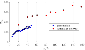
(a)

Figure 11: Local Reynolds number ($Re_{\lambda}$) along the jet centreline as a function of the streamwise distance $x/h$. $Re_{G}=20000$ for the present data. $Re_{G}=42800$ for the data of Antonia et al. (1980).

4.1 Comparison with previously published data

We now compare our data for the centreline mean flow velocity $u_{0}$ and the jet width $\delta$ with data in the published literature.

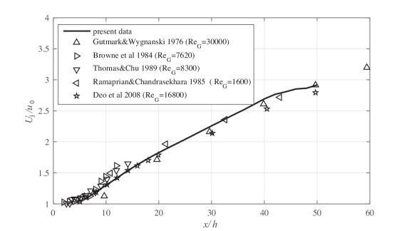
Figure 12: Centreline mean flow velocity $u_{0}$ as a function of the streamwise distance. Data are normalized using the inlet speed $U_{J}$ and are plotted as $U_{J}/u_{0}$ versus $x/h$. The continuous line is representative of the current dataset and symbols refer to previous investigations. Our data show a rather good agreement with Deo et al. (2008), Gutmark & Wygnanski (1976) and Ramaprian & Chandrasekhara (1985) between $x/h$ about 10 and $x/h=50$ (except for a data point by Gutmark & Wygnanski (1976) near $x/h=10$ which is 5% off). Some discrepancies can be detected at distances shorter than $x/h\approx 15$, which are not too far from the potential core, the length of which, as discussed by Deo et al. (2008), is a decreasing function of inlet Reynolds number; some small differences (smaller than 5%) can be detected with the data of Thomas & Chu (1989) and Browne et al. (1984), which are characterized by a significantly smaller $Re_{G}$ and are in the region $x/h\leq 15$.

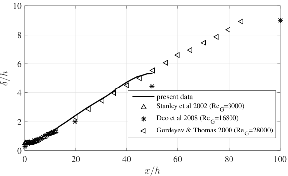
Figure 13: Comparison of the jet width $\delta(x)$ defined in eq. (5) between present measurements and previously published data. Our data compare very well with those of Gordeyev & Thomas (2000) and Stanley et al. (2002). A larger discrepancy between our data and the data of Gordeyev & Thomas (2000) on the one hand and the data of Deo et al. (2008) on the other is detected at $x/h=50$.

Figure 12 shows the mean velocity $u_{0}$ measured along the jet centreline normalized with the inlet speed and plotted as $U_{J}/u_{0}$ versus normalised distance from inlet, $x/h$. Data from the present experiment (continuous line) are compared to different experiments with inlet Reynolds number ranging from values as low as $Re_{G}=1600$ to $Re_{G}=30000$ (see legend of Figure 12). Our data compare very well with Deo et al. (2008), Gutmark & Wygnanski (1976) and Ramaprian & Chandrasekhara (1985) in the range $10<x/h<50$, with differences smaller than 3%. At shorter distances, some discrepancies can be detected but these positions are quite close to the potential core, which as discussed at length by Deo et al. (2008) depends significantly on inlet conditions, including inlet Reynolds number. Also, some discrepancies, smaller than 5%, can be detected with the results of Thomas & Chu (1989) and Browne et al. (1984) in the region $x/h\leq 15$.

Figure 13 shows a comparison of our measured values of the jet width with those obtained in previous investigations: an extremely good matching can be ascertained through the whole domain, particularly with the experimental data of Gordeyev & Thomas (2000) and the numerical simulation of Stanley et al. (2002). Some differences are detected with the data of Deo et al. (2008), but a thorough comparison with their data cannot be carried out given the small number of streamwise locations where they reported jet width measurements (four locations in the range $0<x/h<100$).

All in all, particularly in the region of greatest interest for the present investigation (i.e. $20\leq x/h\leq 50$), the overall behaviours of our centreline mean flow velocity and jet width data do agree quite well with previously published literature.

5 Turbulence dissipation scaling

The global/inlet Reynolds number $Re_{G}$ differs by a factor higher than 2 between our data and the data of Antonia et al. (1980). Nevertheless, figure 8 shows that our data for $C_{\varepsilon}Re_{\delta}$ collapse quite closely with those of Antonia et al. (1980) if $C_{\varepsilon}Re_{\delta}$ is divided by $Re_{G}$ and is plotted as $C_{\varepsilon}Re_{\delta}/Re_{G}$. This is what one would expect from eq. (16) with $m=1$ if the centreline $u^{\prime 2}$ scales as $K_{0}$. It is known that the ratio of the two transverse rms velocities $v^{\prime}/w^{\prime}$ is about constant with $x/h$ in most free turbulent shear flows (Townsend, 1976), and it has been confirmed for turbulent planar jets that $v^{\prime 2}/w^{\prime 2}$ is indeed constant and in fact very close to unity on the centreline (Bashir & Uberoi, 1975, Gutmark & Wygnanski, 1976). With our XW measurements we accessed both $u^{\prime 2}$ and $v^{\prime 2}$, and in figure 14(a) we plot $v^{\prime}/u^{\prime}$ versus $x/h$ on the centreline. The ratio $v^{\prime}/u^{\prime}$ remains about constant around the value $v^{\prime}/u^{\prime}\approx 0.9$ in the range $14\leq x/h\leq 54$. It is therefore reasonable to expect the centreline $u^{\prime 2}$ to approximately scale as $K_{0}$ in the jet experiment of Antonia et al. (1980) and the support for $C_{\varepsilon}\sim Re_{\delta}^{-1}$ in Figure 8 provided by their data to actually be support for eq. (16) with $m=1$ in the range $40\leq x/h\leq 140$.

We now use our own data to test eq. (16). We estimate the centreline dissipation by calculating $\varepsilon_{iso}$ on the centreline and the centreline turbulent kinetic energy as $K_{0}={1\over 2}(u^{\prime 2}+2v^{\prime 2})$ given that we can assume $v^{\prime 2}=w^{\prime 2}$ on the centreline. We plot the results of these centreline calculations in figure 14(b) as $U_{J}h\varepsilon_{iso}\delta^{2}/K_{0}$ and as $\varepsilon_{iso}\delta/K_{0}^{3/2}$, which would be constant in $x/h$ if eq. (16) were to hold with $m=0$. It is quite clear from figure 14(b) that $\varepsilon_{iso}\delta/K_{0}^{3/2}$ is, overall, a decreasing function of $x/h$ and therefore not a constant in the range $20\leq x/h\leq 50$. As can be seen in figure 8, $(U_{J}h)\varepsilon_{iso}\delta^{2}/K_{0}$ cannot be expected to be close to a constant in the very near field $x/h\leq 20$, but figure 14(b) shows that it is definitely constant in the range $20\leq x/h\leq 50$. These results support eq. (16) with $m=1$, i.e. the non-equilibrium dissipation scalings. On the basis of our data and the data of Antonia et al. (1980) we conclude that eq. (16) with $m=1$ is well supported in the region $20\leq x/h\leq 140$. Further studies will be needed in the future to explore dissipation scalings in the region beyond $x/h=140$.

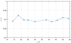
(a)

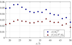
(b)

Figure 14: (a) $v^{\prime}/u^{\prime}$ versus $x/h$ on the centreline. (b) Centreline dissipation coefficient $\epsilon_{iso}\delta/K_{0}^{3/2}$ (blue circles) and $U_{J}h\epsilon_{iso}\delta^{2}/K_{0}$ (red triangles) versus streamwise distance $x/h$ on the centreline. The inlet Reynolds number is $Re_{G}=20000$ and $K_{0}$ is estimated from the centreline $u^{\prime 2}$ and $v^{\prime 2}$ by using $K_{0}={1\over 2}(u^{\prime 2}+2v^{\prime 2})$.

Given that the turbulence dissipation is determined by the turbulence cascade (Vassilicos, 2015; Goto & Vassilicos, 2016) which occurs over about one turnover time, it is worth checking that the streamwise range where eq. (16) holds with $m=1$ is long enough for the turbulence to evolve by at least a few turnover times over this range. We therefore estimate the number of turnover times, $t_{e}$, on the centreline as follows:

$$t_{e}(x)=\frac{1}{u_{0}}\int_{x_{1}}^{x}\,\frac{u^{\prime}}{L_{uu}}dx$$ (24)

where the integral is computed along the centreline and $x_{1}$ is an arbitrary starting point. Figure 15, where we plot $t_{e}$ versus $x/h$, shows that the distance between $x=20h$ and $x=54h$ corresponds to about three turnover times for the present paper’s data.

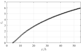
Figure 15: Eddy turnover time $t_{e}$ as a function of the normalised streamwise distance $x/h$ on the centreline. The integral in eq. (24) has been calculated by setting $x_{1}=5h$. The inlet Reynolds number is $Re_{G}=20000$.

6 Self-similarity

Besides the turbulence dissipation scaling (eq. 16), the other assumptions of the theory in section 2 which are accessible by our experiment are the self-similarity of the $U$ profile, which implies that the profiles of $V$ and $R_{xy}$ are also self-similar, the self-similarities of the profiles of $K$ and $\varepsilon$, and $K_{0}\sim R_{0}$ which is only needed if $m\not=1$. In figures 16 and 17 we plot profiles of these five quantities against the similarity coordinate $y/\delta$ normalised by the respective maximum values at each streamwise distance $x$ ($V$ is actually normalized by the innermost maximum value, without loss of generality as long as the profile is self-similar). The turbulent kinetic energy in 16(d) is estimated as $K={1\over 2}(u^{\prime 2}+2v^{\prime 2})$. The turbulence dissipation is estimated as $\varepsilon_{iso}$ in figure 17(a) and as $\varepsilon_{XW}$ in figure 17(b). The results support self-similarity of these profiles from $x=18h$ to the furthermost streamwise distance of our measurements, i.e. $x=54h$: $\varepsilon_{iso}$ and $\varepsilon_{XW}$ appear equally self-similar in this range.

In summary, our data support the self-similarities of $U$, $V$, $R_{xy}$, $K$ and $\varepsilon$ as well as the dissipation scaling (eq. 16) with $m=1$ in the range $20\leq x/h\leq 50$ (perhaps even $18\leq x/h\leq 50$). If we assume that the self-similarities of the $U$, $V$, $R_{xy}$, $K$ and $\varepsilon$ profiles extend further downstream, then the validity of the non-equilibrium self-similar theory of high Reynolds number turbulent planar jets may reach till at least $x/h=140$ given the results of sections 3.2 and 5.

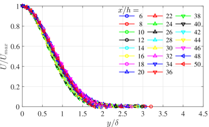
(a)

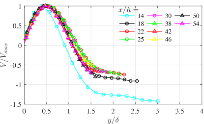
(b)

(c)

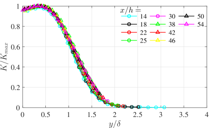
(d)

Figure 16: Self-similarity of (a) $U$, (b) $V$, (c) Reynolds shear stress and (d) turbulent kinetic energy. The data are normalised by their maximum values and plotted as functions of normalised cross-stream coordinate $y/\delta(x)$. Streamwise mean flow data (a) are shown starting from $x$=6$h$ with 2$h$ spacing. Data in (b), (c) and (d) are acquired using the XW in the range $x$=14$h$-54$h$. The inlet Reynolds number is $Re_{G}=20000$.

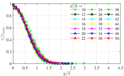
(a)

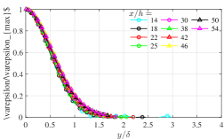
(b)

Figure 17: Turbulent dissipation $\varepsilon$ normalised by its maximum value versus $y/\delta(x)$. (a) Obtained from SW data as $\varepsilon=\varepsilon_{ISO}$. (b) Obtained from XW data as $\varepsilon=\varepsilon_{XW}=\nu(3\overline{(\partial u/\partial x)^{2}}+6\overline{(\partial v/\partial x)^{2}})$. The inlet Reynolds number is $Re_{G}=20000$.

As a final comment for this section, the theory of section 2 is inconclusive if $m\not=1$, in which case eqns. (17)-(18)-(19) are obtained by making the additional assumption $K_{0}\sim R_{0}$. In Figure 18 the ratio of the maximum value of $K$ to the maximum value of the Reynolds shear stress $R_{xy}$ suggests that this extra condition is satisfied for $x/h\geq 25$.

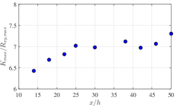
Figure 18: Maximum of $K$ divided by the maximum of $R_{xy}$ (both maxima over all values of $y$ at a given $x$). This ratio $K_{max}/R_{xy,max}$ is plotted as a function of the streamwise distance $x/h$. Data obtained at $Re_{G}=20,000$.

7 Scalings

Having found experimental support for the self-similarity of $U$ and the self-similar behaviours of $R_{xy}$ and $V$ that it implies, we now turn our attention to the George scaling $R_{0}\sim u_{0}^{2}d\delta/dx$ (George, 1989). This scaling is also a consequence of the self-similarity of $U$ and it differs in general from the scaling $R_{0}\sim u_{0}^{2}$ that one finds in various textbooks (e.g. Tennekes & Lumley, 1972). The theory of section 2 makes it clear, however, that one particular instance where $d\delta/dx$ is constant and these two $R_{0}$ scalings are the same is when $K_{0}$ is proportional to $R_{0}$ and the centreline dissipation scales as $D_{0}\sim(Re_{G}/Re_{\delta})^{m}K_{0}^{3/2}/\delta$ with $m=0$. In other words, if the collapse of $R_{xy}/u_{0}^{2}$ profiles differs from the collapse of $R_{xy}/(u_{0}^{2}d\delta/dx)$ profiles (both versus $y/\delta$) and if $K_{0}\sim R_{0}$, then $m\neq 0$. Figure 19 shows clearly that $R_{0}$ does not scale with $u_{0}^{2}$, and also provides support for $R_{0}\sim u_{0}^{2}d\delta/dx$ in the range $18\leq x/h\leq 54$. Given figure 18 which suggests that $K_{0}\sim R_{0}$ holds for $x/h\geq 25$, this is additional support for $m\neq 0$, in agreement with our conclusion concerning $\varepsilon$ in section 5.

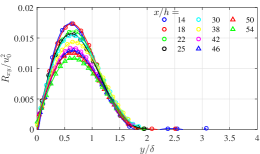
(a)

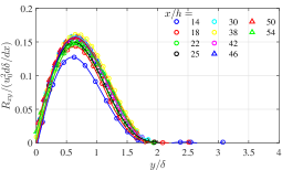
(b)

Figure 19: Reynolds shear stress $R_{xy}$ normalized by (a) $u_{0}^{2}$ and (b) by $u_{0}^{2}\frac{d\delta}{dx}$ as in the George scaling $R_{0}\sim u_{0}^{2}\frac{d\delta}{dx}$. Values of $\frac{d\delta}{dx}$ are obtained by fitting our $\delta(x)$ data with a power law and then differentiating the resulting fit. The profiles are plotted against $y/\delta(x)$. Data acquired for inlet Reynolds number $Re_{G}=20000$.

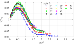
(a)

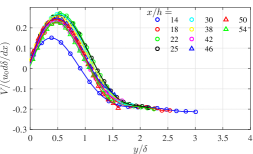
(b)

Figure 20: Mean cross-stream velocity $V$ normalized by (a) $u_{0}$ and (b) $u_{0}\frac{d\delta}{dx}$. Values of $\frac{d\delta}{dx}$ are obtained by fitting our $\delta(x)$ data with a power law and then differentiating the resulting fit. The profiles are plotted against $y/\delta(x)$. Data acquired for inlet Reynolds number $Re_{G}=20000$. In (a) the dashed line is representative of the mean cross-stream velocity profile from the numerical simulation of Stanley et al. (2002) at $x/h=11$ and $Re_{G}=3000$.

Another important implication of the theory involves the mean cross-stream velocity $V(x,y)$ which is self-similar with $v_{0}(x)\sim u_{0}(x)d\delta/dx$, see eq. (7) and eq. (8), if $U(x,y)$ is self-similar. As already mentioned, $d\delta/dx$ is different depending on the value of $m$: $d\delta/dx=const$ for $m=0$ but $d\delta/dx\sim(x-x_{0})^{-1/3}$ for $m=1$. In figure 20(a) we plot the mean cross-stream velocity profiles scaled according to the classical dissipation formula corresponding to $m=0$ and in figure 20(b) we plot the same profiles but scaled according to the non-equilibrium dissipation formula corresponding to $m=1$. The data collapse significantly better in figure 20(b) than in figure 20(a) in the range $18\leq x/h\leq 54$. (In 20(a) we also plot DNS data from Stanley et al., 2002 for comparison, see dashed line.)

The last scalings of the theory in section 2 to be checked are those of the self-similar mean flow profiles, namely the dependencies on $x$ of $u_{0}$ and $\delta$, which can also help us assess $v_{0}(x)\sim u_{0}(x)d\delta/dx$ more closely. The theoretical predictions for $u_{0}$ and $\delta$ when the dissipation scaling is $D_{0}\sim(Re_{G}/Re_{\delta})K_{0}^{3/2}/\delta$ (i.e. $m=1$ in eq. (16) as evidenced by our data and the data of Antonia et al., 1980) are given by equations (17)-(18) with $a=1/3$. These predictions are based on the self-similarity behaviours of $U$, $\varepsilon$ and $K$ which are supported by the experimental results in the previous section. We therefore expect our data to be consistent with eq. (17)-18) and $a=1/3$.

For consistency with the method followed in section 3, we first seek the virtual origins $x_{0,A}$ and $x_{0,B}$ which, respectively, best fit our $u_{0}(x)$ and $\delta(x)$ data in the range $18\leq x/h\leq 50$. We limit ourselves to this range because our SW measurements do not extend downstream of $x/h=50$ and because the non-equilibrium dissipation scaling $D_{0}\sim(Re_{G}/Re_{\delta})K_{0}^{3/2}/\delta$ holds downstream of about $x/h=18$ or $20$. In figure 21 we plot the resulting $x_{0,A}$ and $x_{0,B}$ for different values of the exponent $a$. Unfortunately, the values of $x_{0,A}$ and $x_{0,B}$ are quite close to each other for all exponents $a$ in the range $1/3\leq a\leq 1/2$ and there is no clear way to chose a value of this exponent on such a basis. All exponents $a$ in this range can and do return good fits of our $u_{0}(x)$ and $\delta(x)$ data with a choice of virtual origins $x_{0,A}$ and $x_{0,B}$ that are quite close to each other in every case.

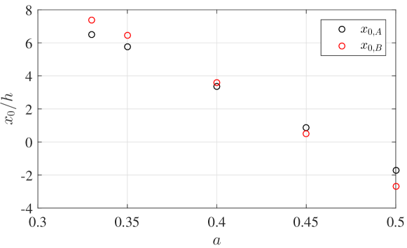
Figure 21: Virtual origins obtained by applying different exponents to the power laws eq. (17) (for $x_{0,A}$) and eq. (18) (for $x_{0,B}$) with $1/3\leq a\leq 1/2$. From our data, acquired for inlet Reynolds number $Re_{G}=20000$.

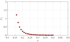
(a)

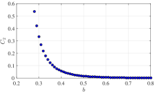
(b)

Figure 22: $C_{1}$ and $C_{2}$ values obtained from linear fits of the derivatives $\frac{d}{dx}(u_{0}(x)/U_{j})^{-1/a}$ and $\frac{d}{dx}(\delta(x)/h)^{1/b}$. From our data, acquired for inlet Reynolds number $Re_{G}=20000$.

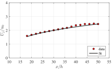
(a)

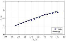
(b)

Figure 23: Fits of the centreline mean flow velocity $u_{0}$ and the jet width $\delta$ according to the non-equilibrium scaling laws given in eqns. (14-15), with fit coefficients given in Table 3. Data acquired for inlet Reynolds number $Re_{G}=20000$.

We therefore turn to the approach of Nedic et al. (2013) which is to estimate the two derivatives $\frac{d}{dx}[(u_{0}(x)/U_{J})^{-1/a}]$ and $\frac{d}{dx}[(\delta(x)/h)^{1/b}]$ for a range of values of $a$ and $b$ and then evaluate the best linear fits of these two derivatives expressed as $C_{1}x/h+A^{-1/a}$ and $C_{2}x/h+B^{1/b}$. The constants $A$ and $B$ are the proportionality constants in $u_{0}(x)/U_{J}=A((x-x_{0,A})/h)^{-a}$ and $\delta(x)/h=B((x-x_{0,B})/h)^{b}$. Again, we apply this analysis to the range $18\leq x/h\leq 50$. In figure 22 we plot the resulting values of $C_{1}$ and $C_{2}$ as functions of $a$ and $b$ respectively. The point of this method is to chose the exponents $a$ and $b$ for which $C_{1}$ and $C_{2}$ vanish. However, it turns out that both $C_{1}$ and $C_{2}$ are very close to 0 for any value of $a$ in the range $1/3\leq a\leq 1/2$ and any value of $b$ in the range $2/3\leq b\leq 1$. The conclusion is therefore the same: any exponents $a$ and $b=2a$ in the range $1/3\leq a\leq 1/2$ can fit our $u_{0}(x)$ and $\delta(x)$ data equally well in the range $18\leq x/h\leq 50$. We have checked that all these good fits can be achieved with values of $x_{0,A}$ and $x_{0,B}$ that are close to each other.

We stress the point that the exponents $a=1/3$ and $b=2a=2/3$, which follow from our definite finding that $m=1$, are consistent with our $u_{0}(x)$ and $\delta(x)$ data. Any other exponents $a$ and $b=2a$ are not in agreement with $m=1$. We therefore set $a=1/3$ and $b=2a=2/3$ and determine the virtual origins $x_{0,A}$ and $x_{0,B}$ and proportionality constants $A$ and $B$ which provide the best fits of our $u_{0}(x)$ and $\delta(x)$ data. We plot our data and our non-equilibrium ($m=1$) fits in Figure 22 and list the values of $x_{0,A}$, $x_{0,B}$, $A$ and $B$ in Table 3. As expected from figure 21, $x_{0,A}$ and $x_{0,B}$ do turn out to be very close to each other, as required by the theory. We repeat that one could fit this data equally well with the classical exponents $a=1/2$ and $b=2a=1$ implied by eq. (19) if $m=0$, including with virtual origins $x_{0,A}$ and $x_{0,B}$ that are very close to each other. The difference is that $m=0$ is not supported by our data and by the data of Antonia et al. (1980) whereas $m=1$ is.

$A$	$a$	$x_{0,A}$	$R^{2}_{u}$	$B$	$b$	$x_{0,B}$	$R^{2}_{\delta}$
1.4	1/3	7.7$h$	0.991	0.48	2/3	8$h$	0.991

Table 3: Fit coefficients for $u_{0}(x)/U_{J}=A((x-x_{0,A})/h)^{-a}$ and $\delta(x)/h=B((x-x_{0,B})/h)^{b}$ where $a$ and $b$ have been set to $a=1/3$ and $b=2a=2/3$. The values of the determination coefficients of the two fits are also reported. From our data which were acquired at inlet Reynolds number $Re_{G}=20000$.

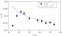
(a)

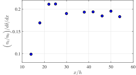
(b)

Figure 24: (a) Streamwise profile of the ratio $v_{0}/u_{0}\sim d{\delta}/dx$. The dashed black line is representative of the $\sim(x-x_{0})^{-1/3}$ power law dependence of $d\delta/dx$ on $x$. The error bars are obtained by repeating the measurements at a given $x/h$ between three and five times; (b) $\frac{v_{0}/u_{0}}{d{\delta}/dx}$ (where ${d{\delta}/dx}$ is obtained from the fit of $\delta(x)$ with the parameters listed in Table 3) plotted as a function of the streamwise distance $x/h$. Data obtained at $Re_{G}=20000$.

We now turn our attention to $v_{0}/u_{0}\sim d\delta/dx$, see eq. (8). Given that the self-similar behaviours of the five profiles studied here are supported by our data in the range $18\leq x/h\leq 54$ and that the dissipation scaling given by $m=1$ is in good agreement with our data for values of $x/h$ larger than about 20, we expect to find $v_{0}/u_{0}\sim d\delta/dx\sim(x/h-x_{0}/h)^{2a-1}$ at values of $x/h$ larger than about 20 with $a=1/3$. In Figure 24(a) we plot $v_{0}/u_{0}$ as a function of $x/h$ and compare it to $(x/h-x_{0}/h)^{-1/3}$ where $x_{0}$ is taken from Table 3 (not fitted anew) as $x_{0}=(x_{0,A}+x_{0,B})/2$ which is very close to both $x_{0,A}$ and $x_{0,B}$. After an initial growth associated with the progressive build-up of entrainment following the potential core, one can see in figure 24(a) a clear streamwise decrease of $v_{0}/u_{0}$ for $x/h>20$ which is evidence that $m\not=0$. As shown in the plots (a) and (b) of figure 24, this decreasing trend is in good agreement with $d\delta/dx\sim(x/h-x_{0}/h)^{-1/3}$ as predicted by the theory for $m=1$. The proportionality coefficient in $d\delta/dx\sim(x/h-x_{0}/h)^{-1/3}$ is obtained from figure 24(b).

We close this section with a comment concerning turbulent viscosity modelling which assumes $R_{xy}$ to equal $-\nu_{T}dU/dy$. The usual algebraic model for the turbulent viscosity $\nu_{T}$ is $\nu_{T}\sim u_{0}\delta$ (see Pope, 2000, Davidson, 2004) and it returns the scalings reported in equations (17)-(18)-(19) with $m=0$ if the mean velocity profiles are assumed to be self-similar. However, in the present case where the data support the non-equilibrium dissipation scaling $D_{0}\sim(Re_{G}/Re_{\delta})K_{0}^{3/2}/\delta$ (i.e. $m=1$) rather than the equilibrium one ($m=0$) and $v_{0}/u_{0}\sim d\delta/dx\sim(x/h-x_{0}/h)^{-1/3}$ rather than $v_{0}/u_{0}=Const$, the turbulent viscosity needs to be $\nu_{T}\sim U_{J}h$ to return the scalings of $u_{0}$ and $\delta$ which are consistent with these non-equilibrium dissipation scalings and self-similarity. The same holds for axisymmetric turbulent wakes where $\nu_{T}\sim u_{0}\delta$ needs to be replaced by $\nu_{T}\sim U_{\infty}L_{B}$ in the presence of the non-equilibrium dissipation scaling (see Dairay et al., 2015 and Obligado et al., 2016), $U_{\infty}$ being the incoming freestream velocity and $L_{B}$ the size of the wake-generating body.

8 Conclusions

The non-equilibrium dissipation law which has been found in grid-generated turbulence (Vassilicos, 2015), axisymmetric turbulent wakes (Obligado et al., 2016), forced and decaying periodic turbulence (Goto & Vassilicos, 2015) and turbulent boundary layers (Nedic et al., 2017) is also present in turbulent planar jets. It does not matter if the local Reynolds number decays with downstream distance like it does in grid-generated turbulence and axisymmetric wakes or grows with downstream distance like it does in turbulent boundary layers and planar jets. In the former case the dissipation coefficient $C_{\varepsilon}$ increases with decreasing local Reynolds number whilst in the latter case it decreases with increasing local Reynolds number. In all cases these increases and decreases happen according to the same inverse power-law relation. This was also observed in the DNS of forced periodic turbulence by Goto & Vassilicos (2015, 2016) where the local Reynolds number undergoes long periods of growth followed by long periods of decline.

Following Townsend (1976), George (1989) and Dairay et al. (2015), the non-equilibrium dissipation law combined with various self-similar profiles imply new centreline mean flow and jet width scalings, see eq. (14) and eq. (15). Our experiments have provided evidence that the profiles of mean flow velocities $U$ and $V$, Reynolds shear stress $R_{xy}$, turbulent kinetic energy $K$ and dissipation $\varepsilon$ are indeed self-similar for streamwise distances downstream of $x=18h$ even though this is not far enough downstream for the memory of inlet conditions to fully fade away. The inlet conditions $U_{J}$ and $h$ are explicitly present in the non-equilibrium dissipation law which is found to hold in a region downstream of $x\approx 20h$ that extends at least as far as $x=140h$ as shown by the data of Antonia et al. (1980). An important implication which our experiment confirms is that the entrainment coefficient $\alpha$ is not constant but decreases as $(x/h-x_{0}/h)^{-1/3}$ over the streamwise extent where the non-equilibrium dissipation law holds.

References

- Antonia et al. (1980) Antonia, R.A., Satyaprakash, B.R. & Hussain, A.K.M.F. 1980 Measurements of dissipation rate and some other characteristics of turbulent plane and circular jets. Physics of Fluids 23, 863055.
- Bashir & Uberoi (1975) Bashir, J. & Uberoi, M.S. 1975 Experiments on turbulent structure and heat transfer in a two-dimensional jet. Physics of Fluids 18, 405.
- Browne et al. (1984) Browne, L., Antonia, R.A. & Chambers, A.J. 1984 The interaction region of a two-dimensional turbulent plane jet. , vol. 149, pp. 355–373.
- Cafiero et al. (2017) Cafiero, G., Castrillo, G., Greco, C.S. & Astarita, T. 2017 Effect of the grid geometry on the convective heat transfer of impinging jets. International Journal of Heat and Mass Transfer 104, 39–50.
- Carlomagno & Ianiro (2014) Carlomagno, G.M. & Ianiro, A. 2014 Thermo-fluid-dynamics of submerged jets impinging at short nozzle-to-plate distance: a review. Experimental Thermal and Fluid Science 58, 15–35.
- Castro (2016) Castro, I.P. 2016 Dissipative distinctions. Journal of Fluid Mechanics 788, 1–4.
- Dairay et al. (2015) Dairay, T., Obligado, M. & Vassilicos, J.C. 2015 Non-equilibrium scaling laws in axisymmetric turbulent wakes. Journal of Fluid Mechanics 781, 166–195.
- Davidson (2004) Davidson, P.A. 2004 Turbulence, An Introduction for Scientists and Engineers. Oxford University Press.
- Deo et al. (2007) Deo, R.C, Mi, J. & Nathan, G.J 2007 The influence of nozzle-exit geometric profile on statistical properties of a turbulent plane jet. Experimental Thermal and Fluid Science 32, 545–559.
- Deo et al. (2008) Deo, R. C., Mi, J. & Nathan, G. J. 2008 The influence of reynolds number on a plane jet. Physics of Fluids 20, 075108.
- Deo et al. (2013) Deo, R. C., Nathan, G. J. & Mi, J. 2013 Similarity analysis of the momentum field of a subsonic, plane air jet with varying jet exit and reynolds number. Physics of Fluids 25, 015115.
- Everitt & Robins (1978) Everitt, K. W. & Robins, A. G. 1978 The development and structure of turbulent plane jets. Journal of Fluid Mechanics pp. 563–583.
- Gardon & Akfirat (1966) Gardon, R. & Akfirat, J.C. 1966 Heat transfer characteristics of impinging two-dimensional air jets. Journal of Heat Transfer pp. 101–107.
- George (1989) George, W.K. 1989 The self-preservation of turbulent flows and its relation to initial conditions and coherent structures. In Advances in Turbulence (ed. W.K. George & R. Arndt). Springer.
- Gordeyev & Thomas (2000) Gordeyev, S.V. & Thomas, F.O. 2000 Coherent structure in the turbulent planar jet. part1. extraction of proper orthogonal decomposition eigenmodes and their self-similarity. Journal of Fluid Mechanics 414, 145–194.
- Goto & Vassilicos (2015) Goto, S. & Vassilicos, J.C. 2015 Energy dissipation and flux laws for unsteady turbulence. Physics Letters A 379.16, 1144–1148.
- Goto & Vassilicos (2016) Goto, S. & Vassilicos, J.C. 2016 Unsteady turbulence cascades. Physical Review E 94, 053108.
- Gutmark & Wygnanski (1976) Gutmark, E. & Wygnanski, I. 1976 The planar turbulent jet. Journal of Fluid Mechanics 73, 465–495.
- Kotsovinos (1977) Kotsovinos, N.E. 1977 Plane turbulent buoyant jets part ii: Turbulence structure. Journal of Fluid Mechanics 81, 45–62.
- Kotsovinos & List (1977) Kotsovinos, N.E. & List, E.J. 1977 Plane turbulent buoyant jets part i: Integral properties. Journal of Fluid Mechanics 81, 25–44.
- Lumley (1992) Lumley, J.L. 1992 Some comments on turbulence. Physics of Fluids A: Fluid Dynamics 4.
- Nedic et al. (2017) Nedic, J., Tavoularis, S. & Marusic, I. 2017 Dissipation scaling in constant-pressure turbulent boundary layers. Physical Review Fluids 2.3, 032601.
- Nedic et al. (2013) Nedic, J., Vassilicos, J.C. & Ganapathisubramani, B. 2013 Axisymmetric turbulent wakes with new nonequilibrium similarity scalings. Physical Review Letters 111, 144503.
- Obligado et al. (2016) Obligado, M., Dairay, T. & Vassilicos, J.C. 2016 Non-equilibrium scaling of turbulent wakes. Physical Review Fluids 1, 044409.
- Pope (2000) Pope, S.B. 2000 Turbulent Flows. Cambridge University Press.
- Ramaprian & Chandrasekhara (1985) Ramaprian, B.R. & Chandrasekhara, M.S. 1985 Lda measurements in plane turbulent jets. Journal of Fluids Engineering 107, 264–271.
- Stanley et al. (2002) Stanley, S.A., Sarkar, S. & Mellado, J.P. 2002 A study of the flow-field evolution and mixing in a planar turbulent jet using direct numerical simulation. Journal of Fluid Mechanics 450, 377–407.
- Tennekes & Lumley (1972) Tennekes, H. & Lumley, J.L. 1972 A first course in turbulence. MIT Press.
- Thomas & Chu (1989) Thomas, F.O. & Chu, H.C. 1989 An experimental investigation of the transition of a planar jet: Subharmonic suppression and upstream feedback. Physics of Fluids 90, 857333.
- Townsend (1976) Townsend, A.A. 1976 The structure of turbulent shear flow. Cambridge University Press.
- Vassilicos (2015) Vassilicos, J.C. 2015 Dissipation in turbulent flows. Annual Review of Fluid Mechanics 47, 95–114.