Large time behavior of a two phase extension of the porous medium equation

Abstract.

We study the large time behavior of the solutions to a two phase extension of the porous medium equation, which models the so-called seawater intrusion problem. The goal is to identify the self-similar solutions that correspond to steady states of a rescaled version of the problem. We fully characterize the unique steady states that are identified as minimizers of a convex energy and shown to be radially symmetric. Moreover, we prove the convergence of the solution to the time-dependent model towards the unique stationary state as time goes to infinity. We finally provide numerical illustrations of the stationary states and we exhibit numerical convergence rates.

Keywords. Two-phase porous media flows, Muskat problem, large time behavior, cross diffusion

AMS subjects classification. 35K65, 35K45, 76S05

1. Introduction

1.1. Presentation of the continuous problem

The purpose of this work is to investigate the large time behavior of a seawater intrusion model which is a two-phase generalization of the porous medium equation (PME). The model we are interested in is derived by Jazar and Monneau in [23], where the authors consider the Dupuit approximation of an unsaturated immiscible two-phase (freshwater and saltwater) within an unconfined aquifer assuming that the interface between both fluids is sharp (the fluids occupy disjoint regions), see also [15, 34] for alternative derivations of the same model. This yields a 2D reduced model obtained from a full 3D model where the unknowns are the heights of the fluid layers. More precisely the interface between the saltwater and the bedrock is set at $\{z=0\}$, whereas the height of the freshwater (resp. saltwater) layer is denoted by $\{z={f}(t,x)\}$ (resp. $\{z={g}(t,x)\}$), see Figure 1. The model proposed in [23] is

(1) $$\begin{cases}\partial_{t}{f}-\nabla{\cdot}\big{(}\nu{f}\nabla({f}+{g})\big{)}=0\quad&\text{in}\quad(0,\infty)\times\mathbb{R}^{2},\\ \partial_{t}{g}-\nabla{\cdot}\big{(}{g}\nabla(\rho{f}+{g})\big{)}=0\quad&\text{in}\quad(0,\infty)\times\mathbb{R}^{2},\\ {f}_{|t=0}={f}_{0},\quad{g}_{|t=0}={g}_{0}\quad&\text{in}\quad\mathbb{R}^{2},\end{cases}$$

where $\rho=\dfrac{\rho_{\text{fresh}}}{\rho_{\text{salt}}}\in(0,1)$ is the density ratio between the two fluids, and where the parameter $\nu=\dfrac{\nu_{\text{salt}}}{\nu_{\text{fresh}}}>0$ is the ratio of the kinematic viscosities.

Figure 1. The physical setting

The authors in [15, 16] studied the classical solutions of system (1). Moreover, the existence of weak solutions is established under different assumptions in [14, 25, 26, 11].

The characteristic time corresponding to the aquifer dynamics is large. Therefore, understanding the large-time behavior of system (1) is of great interest. The so-called entropy method [5, 24] provides a powerful approach to study the long time behavior of different systems of PDEs. It has been developed first for kinetic equations (Boltzmann and Landau [32]). Then it was extended to other problems, as the linear Fokker-Planck equation [9], the porous medium equation (PME) [10, 33], reaction-diffusion systems [12, 13, 21], drift-diffusion systems for semiconductor devices [18, 19, 20], and thin film models [8]. For more details about this method and its application domains, one can refer to [5, 24] and the references therein. Similar results were obtained in [6, 7, 29, 35] based on the interpretation of the PDE models as the gradient flow of a certain energy functional with respect to the Wasserstein metric. We refer for instance to the monographs [3, 30] for an extensive discussion on this topic.

In [27], Laurençot and Matioc studied the large-time behavior of the system (1) in the one-dimensional case. In their paper a classification of self-similar solutions is first provided : there is always a unique even self-similar solution (also found in [34]) while a continuum of non-symmetric self similar solutions exists for certain fluid configurations. The authors proved the convergence of all nonnegative weak solutions towards a self-similar solution. Nevertheless nothing is known about the rate of convergence. Surprisingly, the situation is simpler in the 2D case, as we shall see below.

As already mentioned, the system (1) can be interpreted as a two-phase generalization of the PME. This can be easily seen by choosing $f\equiv 0$ or $g\equiv 0$ in the system (1). In order to explain the principles of the entropy method, let us consider the following PME

(2) $$\begin{cases}\partial_{t}v=\Delta v^{2}\quad&\text{in}\;(0,\infty)\times\mathbb{R}^{2},\\ v(0,x)=v_{0}(x)\geq 0\quad&\text{in}\;\mathbb{R}^{2}.\end{cases}$$

A further transformation of (2) involves the so-called self-similar variables (see [10, 33]) and reads

(3) $$u(t,x)=e^{2t}v\Big{(}\dfrac{1}{4}(e^{4t}-1),xe^{t}\Big{)},\qquad(t,x)\in[0,\infty)\times\mathbb{R}^{2},$$

which transforms (2) into the nonlinear Fokker-Planck equation

(4) $$\begin{cases}\partial_{t}u=\text{div}(xu+\nabla u^{2})\quad&\text{in}\;(0,\infty)\times\mathbb{R}^{2},\\ u(0,x)=v_{0}(x)\geq 0\quad&\text{in}\;\mathbb{R}^{2}.\end{cases}$$

In [10] the authors study the large time behavior of the PME (2) using the rescaled equation (4). The energy corresponding to (4) is

(5) $$H(u)=\int_{\mathbb{R}^{2}}\Big{(}|x|^{2}u+2u^{2}\Big{)}\mathop{}\!\mathrm{d}x.$$

Given a nonnegative initial condition $v_{0}\in L^{1}(\mathbb{R}^{2})$ with $M:=\|v_{0}\|_{L^{1}(\mathbb{R}^{2})}>0$, they prove that the unique stationary solution of (4), which is given by the Barenblatt-Pattle type formula

(6) $$u_{\infty}(x)=\max\Bigg{\{}\beta-\dfrac{1}{4}|x|^{2},0\Bigg{\}},\qquad x\in\mathbb{R}^{2},$$

where $\beta$ is determined by $\|u_{\infty}\|_{L^{1}(\mathbb{R}^{2})}=M$ attracts the corresponding solution $u$ to (4) at an exponential rate. Moreover $u_{\infty}$ is the unique minimizer of $H$ in

$$\Big{\{}u\in L^{2}(\mathbb{R}^{2})\cap L^{1}\big{(}\mathbb{R}^{2},(1+|x|^{2})\mathop{}\!\mathrm{d}x\big{)}\;\;:\;\;\|u\|_{L^{1}(\mathbb{R}^{2})}=M\Big{\}}.$$

More precisely, the relative entropy of $u$ with respect to $u_{\infty}$ is then defined by

$$H(u|u_{\infty}):=H(u)-H(u_{\infty})\geq 0,$$

whereas the entropy production for $H(u|u_{\infty})$ is given by

$$I(u)=\int_{\mathbb{R}^{2}}u\big{|}x+2\nabla u\big{|}^{2}\mathop{}\!\mathrm{d}x.$$

Let the initial data $v_{0}$ satisfy $v_{0}\in L^{1}(\mathbb{R}^{2})\cap L^{\infty}(\mathbb{R}^{2})$ with $|x|^{2+\delta}v_{0}\in L^{1}(\mathbb{R}^{2})$ for some $\delta>0$. Then the corresponding solution $u$ to (4) satisfies

$$\lim_{t\to\infty}H(u(t)|u_{\infty})=0\quad\text{and}\quad\lim_{t\to\infty}I(u(t))=0.$$

Moreover, $H(u(t)|u_{\infty})$ and $I(u(t))$ are linked by the relation

(7) $$\dfrac{\mathop{}\!\mathrm{d}}{\mathop{}\!\mathrm{d}t}H(u(t)|u_{\infty})=-2I(u(t)),$$

and

(8) $$\dfrac{\mathop{}\!\mathrm{d}}{\mathop{}\!\mathrm{d}t}I(u(t))=-2I(u(t))-R(t),$$

where $R(t)\geq 0$. Combining (7) and (8) one obtains

(9) $$\dfrac{\mathop{}\!\mathrm{d}}{\mathop{}\!\mathrm{d}t}H(u(t)|u_{\infty})=\dfrac{\mathop{}\!\mathrm{d}}{\mathop{}\!\mathrm{d}t}I(u(t))+R(t)\geq\dfrac{\mathop{}\!\mathrm{d}}{\mathop{}\!\mathrm{d}t}I(u(t)).$$

Integrating (9) with respect to $t$ over $(0,\infty)$ gives

(10) $$0\leq H(u(t)|u_{\infty})\leq I(u(t)),\quad t>0.$$

Substituting (10) into (7), one concludes with the exponential decay of the relative entropy to zero at a rate 2.

The goal of this paper is to apply a similar strategy to describe the long time behavior of the system (1). Our approach relies also in the use of self-similar variables (12), leading to the introduction of quadratic confining potentials. The advantage of this alternative formulation is that the profiles of nonnegative self-similar solutions to (1) are nonnegative stationary solutions to (13). We will give an explicit characterization of the self-similar profiles in Section 4 and, relying on compactness arguments, we prove the convergence towards a stationary solution. Unfortunately, due to the extended complexity of the problem (1) with respect to (2) we are not able to establish the exponential convergence towards a steady state. This motivates the numerical investigation carried out in Section 5, using a Finite Volume scheme [2, 1] which preserves at the discrete level the main features of the continuous problem (in particular the nonnegativity of the solutions, conservation of mass and decay of energy).

The outline of the paper is as follows. In the next section we state the main results of our paper. As a preliminary step, we introduce a rescaled version (13) of the system (1) which relies in particular on the introduction of self-similar variables. In Theorem 2.1 we state the existence and uniqueness of nonnegative stationary solutions to (13), which are moreover radially symmetric, compactly supported and Lipschitz continuous. The convergence of any nonnegative weak solution to (13) towards these stationary solutions is stated in Theorem 2.2. In Section 3 we prove Theorem 2.1 and Theorem 2.2. In Section 4 we give a classification of the self-similar profiles and we exhibit critical values of the parameter $\nu$ for which the shape of the stationary profile changes. We finally present in Section 5 numerical simulations for different values of $\nu$ in order to observe the stationary solutions and the decay of the relative energy.

2. Main results

In what follows, given $M>0$, we use the following closed convex set

$$\mathcal{K}_{M}:=\Big{\{}h\in L^{2}(\mathbb{R}^{2})\cap L^{1}\big{(}\mathbb{R}^{2},(1+|x|^{2})\mathop{}\!\mathrm{d}x\big{)}:\ h\geq 0\;\;\text{a.e. and}\;\;\|h\|_{L^{1}(\mathbb{R}^{2})}=M\Big{\}}.$$

2.1. Self-similar solutions

The main contribution of this paper is the classification of nonnegative self-similar solutions to (1), that is, solutions of the form

(11) $$({f},{g})(t,x)=(1+t)^{-1/2}(F,G)(x(1+t)^{-1/4}),\quad(t,x)\in(0,\infty)\times\mathbb{R}^{2}.$$

Deeper insight on this issue is provided by transforming (1) using the so-called self-similar variables [10, 33], i.e.,

(12) $$({f},{g})(t,x)=\dfrac{1}{(1+t)^{1/2}}(\tilde{f},\tilde{g})\Big{(}\log(1+t),\dfrac{x}{(1+t)^{1/4}}\Big{)}.$$

We end up with the following rescaled system

(13) $$\begin{cases}\partial_{t}\tilde{f}-\nabla{\cdot}\Big{(}\nu\tilde{f}\nabla(\tilde{f}+\tilde{g}+b/\nu)\Big{)}=0\quad&\text{in}\quad(0,\infty)\times\mathbb{R}^{2},\\ \partial_{t}\tilde{g}-\nabla{\cdot}\Big{(}\tilde{g}\nabla(\rho\tilde{f}+\tilde{g}+b)\Big{)}=0\quad&\text{in}\quad(0,\infty)\times\mathbb{R}^{2},\\ \tilde{f}_{|t=0}=f_{0},\quad\tilde{g}_{|t=0}=g_{0}\quad&\text{in}\quad\mathbb{R}^{2},\end{cases}$$

where $b(x)=|x|^{2}/8$. Thus this change of variable preserves the nature of the equations but adds a confining drift term, the confining potentials $b/\nu$ and $b$ being different as soon as the two phases have different kinematic viscosities, i.e., $\nu\neq 1$. The resulting system (13) still has a gradient flow structure, but for a modified energy in comparison to (1). Indeed the system (13) can be interpreted as the gradient flow with respect to the $2-$Wasserstein metric [25] of the following energy

(14) $$\mathfrak{E}(\tilde{f},\tilde{g})=\int_{\mathbb{R}^{2}}E(\tilde{f},\tilde{g})\mathop{}\!\mathrm{d}x,$$

where

(15) $$E(\tilde{f},\tilde{g})=\dfrac{\rho}{2}(\tilde{f}+\tilde{g})^{2}+\dfrac{1-\rho}{2}\tilde{g}^{2}+b\Big{(}\dfrac{\rho}{\nu}\tilde{f}+\tilde{g}\Big{)}.$$

A corner stone of our study is that, if $(f,g)$ is a self-similar solution (11) to (1), then the corresponding self-similar profile $(F,G)$ is a stationary solution to (13). We will see in what follows that, given $M_{f}>0$ and $M_{g}>0$, there is a unique nonnegative stationary solution $(F,G)$ to (13) satisfying $\|F\|_{L^{1}(\mathbb{R}^{2})}=M_{f}$ and $\|G\|_{L^{1}(\mathbb{R}^{2})}=M_{g}$ and it is the unique minimizer of $\mathfrak{E}$ in $\mathcal{K}_{M_{f}}\times\mathcal{K}_{M_{g}}$. Furthermore, it satisfies the system

$$\begin{cases}F\nabla\phi_{F}&=0\quad\text{in}\quad\mathbb{R}^{2},\\ G\nabla\phi_{G}&=0\quad\text{in}\quad\mathbb{R}^{2},\end{cases}$$

where we introduce the potentials

$$\phi_{F}:=F+G+\frac{b}{\nu},\qquad\phi_{G}:=\rho F+G+b.$$

In other words, the fluxes expressed in the self-similar variables are identically equal to zero.

In what follows, we mainly work on the system (13) expressed in self-similar variables. In order to lighten the notations, we remove the tildes on $\tilde{f}$ and $\tilde{g}$ and denote solutions to (13) by $(f,g)$ while the steady states to (13) are denoted by $(F,G)$.

Given two positive real numbers $M_{f}>0$ and $M_{g}>0$ and a stationary solution $(F,G)\in\mathcal{K}_{M_{f}}\times\mathcal{K}_{M_{g}}$ to (13), we define the positivity sets $E_{F}$ and $E_{G}$ of $F$ and $G$ by

$$E_{F}=\{x\in\mathbb{R}^{2}\;:\;F(x)>0\},\quad E_{G}=\{x\in\mathbb{R}^{2}\;:\;G(x)>0\},$$

and notice that $E_{F}$ and $E_{G}$ are both nonempty as

(16) $$\|F\|_{L^{1}(\mathbb{R}^{2})}=\int_{\mathbb{R}^{2}}F\mathop{}\!\mathrm{d}x=M_{f}>0\quad\text{and}\quad\|G\|_{L^{1}(\mathbb{R}^{2})}=\int_{\mathbb{R}^{2}}G\mathop{}\!\mathrm{d}x=M_{g}>0.$$

2.2. Main results

Let $(F,G)\in\mathcal{K}_{M_{f}}\times\mathcal{K}_{M_{g}}$ be a stationary solution of (13). Let $M_{f}>0$ and $M_{g}>0$ be two positive real numbers.

Theorem 2.1 (Self-similar profiles).

There exists a unique stationary solution $(F,G)\in\mathcal{K}_{M_{f}}\times\mathcal{K}_{M_{g}}$ of (13) such that $F$ and $G$ belong to $H^{1}(\mathbb{R}^{2})$ and $\sqrt{F}\phi_{F}$ and $\sqrt{G}\phi_{G}$ belong to $L^{2}(\mathbb{R}^{2})$. It is radially symmetric, compactly supported, and Lipschitz continuous, and satisfies

$$\begin{cases}F\nabla(F+G+b/\nu)&=0\quad\text{a.e. in}\quad\mathbb{R}^{2},\\ G\nabla(\rho F+G+b)&=0\quad\text{a.e. in}\quad\mathbb{R}^{2}.\end{cases}$$

Moreover, $E_{F}$ and $E_{G}$ are bounded connected sets and

$$(F,G)\in\underset{(f,g)\in\mathcal{K}_{M_{f}}\times\mathcal{K}_{M_{g}}}{\operatorname{arg\,min}}\mathfrak{E}(f,g).$$

An important result of this paper is the complete classification of the self-similar profiles $(F,G)$. In fact, in contrast with the 1D case [27], we prove that all self-similar profiles $(F,G)$ are radially symmetric and thus can be computed explicitly, see Section 4. Besides being of interest to compare the outcome of numerical simulations with the theoretical predictions, this feature is at the heart of the uniqueness proof. Still, as it will be explained in Section 4, the shape of $F$ and $G$ strongly depends on $\nu$, $\rho$, and the mass ratio ${M_{f}}/{M_{g}}$. The topology of $E_{F}$ and $E_{G}$ changes according to the values of these parameters.

The second result concerns the convergence of weak solutions to (13) towards the stationary state.

Theorem 2.2 (Convergence towards the stationary state).

Let $(f_{0},g_{0})\in\mathcal{K}_{M_{f}}\times\mathcal{K}_{M_{g}}$ and consider the weak solution $(f,g)$ of (13) given by Theorem 3.2. Then

$$\big{(}f(t),g(t)\big{)}\longrightarrow(F,G)\;\text{ in }\;L^{2}(\mathbb{R}^{2};\mathbb{R}^{2})\;\text{ as }\;t\rightarrow\infty,$$

where $(F,G)$ is the unique stationary solution of (13) in $\mathcal{K}_{M_{f}}\times\mathcal{K}_{M_{g}}$ given by Theorem 2.1.

Theorem 2.2 guarantees the convergence of the solutions of (13) to the steady state but provides no information on the rate of convergence. We conclude the paper by a numerical investigation concerning the convergence speed. The situation appears to be more intricate than for the (rescaled) single phase PME (4) and, even though exponential convergence is always observed in our numerical tests, the rate strongly varies with the data and goes close to zero for some values of $\nu$. It is in particular rather unclear if there exists a uniform strictly positive minimum decay rate at which convergence occurs.

3. The steady states and convergence towards a minimizer

We fix $M_{f}>0$ and $M_{g}>0$.

3.1. Energy/energy dissipation for weak solutions

Let $\omega\in L^{1}_{\rm loc}(\mathbb{R}^{2};\mathbb{R}_{+})$ with $\mathbb{R}_{+}=(0,\infty)$. For $r\geq 1$, we define $L^{r}_{\omega}(\mathbb{R}^{2})$ as the set of measurable functions $\psi$ such that

$$\int_{\mathbb{R}^{2}}|\psi(y)|^{r}\omega(y)\mathop{}\!\mathrm{d}y<\infty,$$

which is a Banach space once equipped with the norm

$$\|\psi\|_{L^{r}_{\omega}(\mathbb{R}^{2})}=\left(\int_{\mathbb{R}^{2}}|\psi(y)|^{r}\omega(y)\mathop{}\!\mathrm{d}y\right)^{1/r}.$$

For further use, we define the phase potentials

(17) $$\phi_{f}=f+g+b/\nu\;\text{ and }\;\phi_{g}=\rho f+g+b.$$

Definition 3.1 (weak solution).

Consider $(f_{0},g_{0})\in\mathcal{K}_{M_{f}}\times\mathcal{K}_{M_{g}}$. A pair $(f,g):\mathbb{R}^{2}\times\mathbb{R}_{+}\to\mathbb{R}_{+}^{2}$ is a weak solution to the problem (13) if

1. $f$ and $g$ belong to $L^{\infty}(\mathbb{R}_{+};L^{2}(\mathbb{R}^{2}))$ and to $L^{\infty}(\mathbb{R}_{+};L^{1}_{|x|^{2}}(\mathbb{R}^{2}))$,

2. $\nabla f$ and $\nabla g$ belong to $L^{2}_{\rm loc}(\mathbb{R}_{+};L^{2}(\mathbb{R}^{2}))$,

3. $\sqrt{f}\nabla\phi_{f}$ and $\sqrt{g}\nabla\phi_{g}$ belong to $L^{2}(\mathbb{R}_{+}\times\mathbb{R}^{2})$

4. for all $\xi\in C^{\infty}_{c}(\mathbb{R}_{+}\times\mathbb{R}^{2})$, there holds

   $$\int_{\mathbb{R}_{+}}\int_{\mathbb{R}^{2}}f\partial_{t}\xi\mathop{}\!\mathrm{d}x\mathop{}\!\mathrm{d}t+\int_{\mathbb{R}^{2}}f_{0}\xi(0,\cdot)\mathop{}\!\mathrm{d}x-\int_{\mathbb{R}_{+}}\int_{\mathbb{R}^{2}}\nu f\nabla\phi_{f}\cdot\nabla\xi\mathop{}\!\mathrm{d}x\mathop{}\!\mathrm{d}t=0,$$

   $$\int_{\mathbb{R}_{+}}\int_{\mathbb{R}^{2}}g\partial_{t}\xi\mathop{}\!\mathrm{d}x{\rm d}t+\int_{\mathbb{R}^{2}}g_{0}\xi(0,\cdot)\mathop{}\!\mathrm{d}x-\int_{\mathbb{R}_{+}}\int_{\mathbb{R}^{2}}g\nabla\phi_{g}\cdot\nabla\xi\mathop{}\!\mathrm{d}x\mathop{}\!\mathrm{d}t=0.$$

The existence of a weak solution of the problem (13) and the decay of the energy $\mathfrak{E}$ are given by the following theorem.

Theorem 3.2.

Consider $(f_{0},g_{0})\in\mathcal{K}_{M_{f}}\times\mathcal{K}_{M_{g}}$. There exists a weak solution in the sense of Definition 3.1. Moreover, it satisfies the energy inequality

(18) $$\mathfrak{E}(f,g)(t)+\int_{s}^{t}\mathcal{I}(f,g)(\tau)\mathop{}\!\mathrm{d}\tau\leq\mathfrak{E}(f,g)(s),\quad t\geq s\geq 0,$$

with the energy dissipation $\mathcal{I}$ given by

(19) $$\mathcal{I}(f,g)=\int_{\mathbb{R}^{2}}\left(\nu\rho f|\nabla\phi_{f}|^{2}+g|\nabla\phi_{g}|^{2}\right)\mathop{}\!\mathrm{d}x,$$

and the entropy inequality

(20) $$\mathcal{H}(f,g)(t)+\int_{s}^{t}\mathcal{D}(f,g)(\tau)\mathop{}\!\mathrm{d}\tau\\ \leq\mathcal{H}(f,g)(s)+\left(\frac{\rho M_{f}}{2}+\frac{\nu M_{g}}{2}\right)(t-s),\quad t\geq s\geq 0,$$

where

$$\mathcal{H}(f,g) =\int_{\mathbb{R}^{2}}\left(\rho f\ln{f}+\nu g\ln{g}\right)\mathop{}\!\mathrm{d}x,$$

$$\mathcal{D}(f,g) =\nu\rho\|\nabla(f+g)\|_{L^{2}(\mathbb{R}^{2})}^{2}+\nu(1-\rho)\|\nabla g\|_{L^{2}(\mathbb{R}^{2})}^{2}.$$

Since $u\log(u)\leq u^{2}$ for $u\geq 0$, one has

(21) $$\mathcal{H}(f,g)(t)\leq\rho\|f(t)\|_{L^{2}(\mathbb{R}^{2})}^{2}+\nu\|g(t)\|_{L^{2}(\mathbb{R}^{2})}^{2},\quad\text{for a.e.}\;t\in\mathbb{R}_{+}.$$

On the other hand, by [4, Eq. (2.14)],

(22) $$\mathcal{H}(f,g)(t)\geq-\pi(\rho+\nu)+\rho\|f(t)\|_{L^{1}_{|x|^{2}}(\mathbb{R}^{2})}+\nu\|g\|_{L^{1}_{|x|^{2}}(\mathbb{R}^{2})},\quad\text{for a.e.}\;t\in\mathbb{R}_{+}.$$

Combining (21) and (22), one gets that $\mathcal{H}(f,g)$ belongs to $L^{\infty}(\mathbb{R}_{+})$, so that (20) makes sense for almost every $t\geq s\geq 0$.

The existence of a weak solution was proven by Laurençot and Matioc in [25, 26] by proving the convergence of a JKO scheme without the confining potentials $b/\nu$ and $b$, but the proof can be extended in the presence of these quadratic confining potentials without particular difficulties. The $L_{\rm loc}^{2}(L^{2})$ estimates on $\nabla f$ and $\nabla g$ and the entropy inequality (20) are obtained thanks to the flow interchange technique of Matthes et al. [28].

An important consequence of Theorem 3.2 is that, if $(F,G)\in\mathcal{K}_{M_{f}}\times\mathcal{K}_{M_{g}}$ is a stationary solution to (13) such that

(23) $$(F,G)\in H^{1}(\mathbb{R}^{2};\mathbb{R}^{2})\;\text{ and }\;(\sqrt{F}\nabla\phi_{F},\sqrt{G}\nabla\phi_{G})\in L^{2}(\mathbb{R}^{2};\mathbb{R}^{4}),$$

then we infer from (18) and the nonnegativity of $\mathcal{I}$ that $\mathcal{I}(F,G)=0$ (recall that $\phi_{F}$ and $\phi_{G}$ are defined by (17)). In other words, $F$ and $G$ have vanishing fluxes and

(24) $$\begin{cases}F\nabla(F+G+b/\nu)&=0\quad\text{in}\quad\mathbb{R}^{2},\\ G\nabla(\rho F+G+b)&=0\quad\text{in}\quad\mathbb{R}^{2}.\end{cases}$$

3.2. Existence and properties of the minimizer of the energy

As already mentioned, the problem (1) can be interpreted as a two phase generalization of the PME (2), and its long time behavior is expected to share some common features with that equation. In particular, since the Barenblatt profile $u_{\infty}$ given by (6) is the unique minimizer of the energy functional (5) under a mass constraint, we are led to consider the following minimization problem

(25) $$\inf_{(f,g)\in\mathcal{K}_{M_{f}}\times\mathcal{K}_{M_{g}}}\mathfrak{E}(f,g).$$

Owing to the energy inequality (18), a minimizer $(F,G)$ of $\mathfrak{E}$ in $\mathcal{K}_{M_{f}}\times\mathcal{K}_{M_{g}}$ is obviously a stationary solution to (13) and thus satisfies (24).

In order to prove the uniqueness of the minimizer in (25), we need the strict convexity of the energy functional $\mathfrak{E}$.

Proposition 3.3.

$\mathfrak{E}$ is a strictly convex function on $\mathcal{K}_{M_{f}}\times\mathcal{K}_{M_{g}}$.

Proof.

If $E$ is strictly convex then $\mathfrak{E}$ is strictly convex. We denote by $D^{2}E$ the Hessian matrix of $E$. Then

$$D^{2}E=\begin{pmatrix}\rho&\rho\\ \rho&1\end{pmatrix}.$$

Recalling that $\rho\in(0,1)$, the matrix $D^{2}E$ is symmetric with $\text{det}(D^{2}E)=\rho(1-\rho)>0$ and $\text{tr}(D^{2}E)=1+\rho>0.$ We deduce that $D^{2}E$ is definite positive and hence $E$ is strictly convex. ∎

Let us now introduce some material that will be needed to prove the existence of a minimizer of (25). There exist $C_{\star}>0$ and $C^{\star}>0$ depending only on $\rho$ and $\nu$ such that

(26) $$C_{\star}(\mathcal{N}(f)+\mathcal{N}(g))\leq\mathfrak{E}(f,g)\leq C^{\star}(\mathcal{N}(f)+\mathcal{N}(g)),$$

where

$$\mathcal{N}(h)=\|h\|^{2}_{L^{2}(\mathbb{R}^{2})}+\|h\|_{L^{1}_{|x|^{2}}(\mathbb{R}^{2})},\quad\text{for}\quad h\in L^{2}(\mathbb{R}^{2})\cap L^{1}_{|x|^{2}}(\mathbb{R}^{2}).$$

Indeed, on the one hand, since $f$, $g$ and $b$ are nonnegative, there holds

$$E(f,g) =\dfrac{\rho}{2}(f+g)^{2}+\dfrac{1-\rho}{2}g^{2}+b(\dfrac{\rho}{\nu}f+g)$$

$$\geq\dfrac{\rho}{2}(f^{2}+\dfrac{1}{\nu}bf)+\dfrac{1}{2}(g^{2}+bg).$$

On the other hand, using $(u+v)^{2}\leq 2(u^{2}+v^{2})$, we have

$$E(f,g)\leq\rho f^{2}+\dfrac{1+\rho}{2}g^{2}+\dfrac{\rho}{\nu}bf+bg,$$

which implies (26). This motivates the introduction of the Banach space

$$X=L^{2}(\mathbb{R}^{2})\cap L^{1}_{|x|^{2}}(\mathbb{R}^{2})\qquad\text{with}\quad\|\cdot\|_{X}=\|\cdot\|_{L^{2}}+\|\cdot\|_{L^{1}_{|x|^{2}}}.$$

We say that a sequence $\left(u_{n}\right)_{n\geq 1}$ converges in $X$ in the weak-$\star$ sense towards $u$ if $u_{n}$ converges to $u$ weakly in $L^{2}(\mathbb{R}^{2})$ and if the densities of the moments of order $2$ $x\mapsto u_{n}(x)|x|^{2}$ converge weakly in the sense of finite measures (i.e., in the dual of the space $C_{0}(\mathbb{R}^{2})$ of the continuous functions decaying to $0$ as $|x|\to\infty$) towards $x\mapsto u(x)|x|^{2}$. Then any bounded sequence in $X$ is relatively compact in $X$ for the weak-$\star$ topology.

We can now go to the following statement.

Proposition 3.4.

There exists a unique minimizer $(F,G)$ of $\mathfrak{E}$ in $\mathcal{K}_{M_{f}}\times\mathcal{K}_{M_{g}}$. Moreover, $F$ and $G$ belong to $H^{1}(\mathbb{R}^{2})$ while $\sqrt{F}\phi_{F}$ and $\sqrt{G}\phi_{G}$ belong to $L^{2}(\mathbb{R}^{2})$ and it satisfies (24), the fluxes $\phi_{F}$ and $\phi_{G}$ being defined in (17).

Proof.

The uniqueness of the minimizer follows from the strict convexity of the energy functional $\mathfrak{E}$ proved in Proposition 3.3.

Let us now prove the existence of a minimizer. To this end, pick a minimizing sequence $(f_{k},g_{k})_{k\geq 1}\in\mathcal{K}_{M_{f}}\times\mathcal{K}_{M_{g}}$. Thanks to (26) there exists a constant $C>0$ such that

(27) $$\|f_{k}\|_{X}+\|g_{k}\|_{X}\leq C,\;\forall k\geq 1.$$

We obtain that there exist $(F,G)\in L^{2}(\mathbb{R}^{2};\mathbb{R}_{+})^{2}$ and a subsequence of $(f_{k},g_{k})_{k\geq 1}$ (denoted again by $(f_{k},g_{k})_{k\geq 1}$) such that

$$f_{k}\to F\;\;\text{weakly-$\star$ in}\;\;X\quad\text{and}\;\;g_{k}\to G\;\;\text{weakly-$\star$ in}\;\;X.$$

This convergence implies in particular that $\|F\|_{L^{1}(\mathbb{R}^{2})}=M_{f}$ and $\|G\|_{L^{1}(\mathbb{R}^{2})}=M_{g}$, hence $(F,G)\in\mathcal{K}_{M_{f}}\times\mathcal{K}_{M_{g}}$.

Moreover, the energy functional $\mathfrak{E}$ is lower semi-continuous for the weak-$\star$ topology of $X$. Thus,

$$\mathfrak{E}(F,G)\leq\underset{k\to\infty}{\rm liminf}\;\mathfrak{E}(f_{k},g_{k}),$$

so that $(F,G)$ is a minimizer of $\mathfrak{E}$ in $\mathcal{K}_{M_{f}}\times\mathcal{K}_{M_{g}}$.

Let us now show that (24) holds. To this end, define $(\check{f},\check{g})$ as a solution of the evolutionary system

(28) $$\begin{cases}\partial_{t}\check{f}-\nabla{\cdot}\Big{(}\nu\check{f}\nabla(\check{f}+\check{g}+b/\nu)\Big{)}=0\quad&\text{in}\quad(0,\infty)\times\mathbb{R}^{2},\\ \partial_{t}\check{g}-\nabla{\cdot}\Big{(}\check{g}\nabla(\rho\check{f}+\check{g}+b)\Big{)}=0\quad&\text{in}\quad(0,\infty)\times\mathbb{R}^{2},\\ \check{f}_{|t=0}=F,\quad\check{g}_{|t=0}=G\quad&\text{in}\quad\mathbb{R}^{2}.\end{cases}$$

Using (18) one has

$$\mathfrak{E}(\check{f},\check{g})(t)+\int_{0}^{t}\mathcal{I}(\check{f},\check{g})(\tau)\mathop{}\!\mathrm{d}\tau\leq\mathfrak{E}(F,G),$$

with

$$\mathcal{I}(\check{f},\check{g})=\int_{\mathbb{R}^{2}}\left(\nu\rho\check{f}|\nabla\phi_{\check{f}}|^{2}+\check{g}|\nabla\phi_{\check{g}}|^{2}\right)\mathop{}\!\mathrm{d}x,$$

where $\phi_{\check{f}}=\check{f}+\check{g}+b/\nu$ and $\phi_{\check{g}}=\rho\check{f}+\check{g}+b$. Since $(F,G)$ is a minimizer of $\mathfrak{E}$ in $\mathcal{K}_{M_{f}}\times\mathcal{K}_{M_{g}}$ and $(\check{f}(t),\check{g}(t))$ belongs to $\mathcal{K}_{M_{f}}\times\mathcal{K}_{M_{g}}$ for all $t\geq 0$, we deduce from the nonnegativity of $\mathcal{I}$ that $\mathfrak{E}(\check{f}(t),\check{g}(t))=\mathfrak{E}(F,G)$ and $\mathcal{I}(\check{f}(t),\check{g}(t))=0$ for a.e. $t>0$. Owing to the minimizing property of $(F,G)$, the first identity readily implies that $(\check{f}(t),\check{g}(t))=(F,G)$ for all $t\geq 0$. On the one hand, it follows from Theorem 3.2 that $(F,G)$ enjoys the regularity properties listed in Proposition 3.4. On the other hand, we conclude that $(F,G)$ satisfies $\mathcal{I}(F,G)=0$ and thus (24). ∎

With Proposition 3.4 at hand, we are now interested in the regularity of stationary solutions $(F,G)$ to (13) in $\mathcal{K}_{M_{f}}\times\mathcal{K}_{M_{g}}$ and in the description of the positivity sets $E_{F}$ and $E_{G}$ of $F$ and $G$ defined by

$$E_{F}=\{x\in\mathbb{R}^{2}\;:\;F(x)>0\},\quad E_{G}=\{x\in\mathbb{R}^{2}\;:\;G(x)>0\}.$$

Lemma 3.5.

Let $(F,G)\in\mathcal{K}_{M_{f}}\times\mathcal{K}_{M_{g}}$ be a solution of (24) enjoying the regularity properties (23). Then

1. $E_{F}\cap E_{G}\neq\emptyset$,

2. $F$ and $G$ are locally Lipschitz continuous and radially symmetric.

Proof.

(i) Assume for contradiction that $E_{F}\cap E_{G}=\emptyset$. Then $F\nabla G=G\nabla F=0$ in $\mathbb{R}^{2}$ and it follows from (24) that $(F,G)$ satisfy the equations

$$\begin{cases}F\nabla(F+b/\nu)&=0\quad\text{in}\quad\mathbb{R}^{2},\\ G\nabla(G+b)&=0\quad\text{in}\quad\mathbb{R}^{2},\end{cases}$$

hence $F$ and $G$ are Barenblatt solutions centred at $0$. Thus $0\in E_{F}\cap E_{G}=\emptyset$, yielding a contradiction.

(ii) Let us prove that $(F,G)$ are locally Lipschitz continuous and radially symmetric. We have

$$\mathbb{R}^{2}=(E_{F}\cap E_{G})\cup(E_{F}\cap E_{G}^{c})\cup(E_{F}^{c}\cap E_{G})\cup(E_{F}^{c}\cap E_{G}^{c}).$$

Since $F$ and $G$ belong to $H^{1}(\mathbb{R}^{2})$ by (23), it follows from Stampacchia’s theorem that

$$\nabla F=0\;\text{a.e. in}\;E_{F}^{c}\quad\text{and}\;\;\nabla G=0\;\text{a.e. in}\;E_{G}^{c}.$$

Therefore

(29) $$\nabla G=-\nabla b\;\;\text{a.e in}\;\;E_{F}^{c}\cap E_{G},\;\nabla F=-\nabla b/\nu\;\;\text{a.e on}\;\;E_{G}^{c}\cap E_{F},$$

(30) $$\nabla F=\dfrac{\nu-1}{\nu(1-\rho)}\nabla b\;\;\text{and}\;\;\nabla G=\dfrac{\rho-\nu}{\nu(1-\rho)}\nabla b\;\;\text{a.e in}\;\;E_{F}\cap E_{G}.$$

Since $\nabla b(x)=x/4$ is locally bounded in $\mathbb{R}^{2}$, both $F$ and $G$ are locally Lipschitz continuous in $\mathbb{R}^{2}$. In addition, $\nabla F(x)\cdot x^{\bot}=\nabla G(x)\cdot x^{\bot}=0$ for almost all $x=(x_{1},x_{2})\in\mathbb{R}^{2}$ with $x^{\bot}=(-x_{2},x_{1})$. Consequently, $F$ and $G$ are radially symmetric. ∎

According to the discussion above the profiles $(F,G)$ of self-similar solutions of (1) defined in (11) are stationary solutions of (13) and satisfy (23) and (24). Moreover $(F,G)$ are radially symmetric. Then we can express $F$ and $G$ as functions of $r=|x|$. Thanks to (29)–(30) one has:

1. On $E_{F}\cap E_{G}$, there are $(C_{1},C_{2})\in\mathbb{R}^{2}$ such that

   (31) $$F(r)=C_{1}+\dfrac{\nu-1}{8\nu(1-\rho)}r^{2},\qquad G(r)=C_{2}+\dfrac{\rho-\nu}{8\nu(1-\rho)}r^{2}.$$

2. On $E_{F}\cap E_{G}^{c}$, there is $C_{3}\in\mathbb{R}$ such that

   (32) $$F(r)=C_{3}-\dfrac{1}{8\nu}r^{2},\qquad G(r)=0.$$

3. On $E_{G}\cap E_{F}^{c}$, there is $C_{4}\in\mathbb{R}$ such that

   (33) $$G(r)=C_{4}-\dfrac{1}{8}r^{2},\qquad F(r)=0.$$

The above statements are actually not completely correct since the quantities $C_{1},C_{2},C_{3}$ and $C_{4}$ are constant only on the connected components of $E_{F}\cap E_{G}$, $E_{F}\cap E_{G}^{c}$, and $E_{G}\cap E_{F}^{c}$, respectively. But this ambiguity will be removed thanks to the following lemma.

Lemma 3.6.

Let $(F,G)\in\mathcal{K}_{M_{f}}\times\mathcal{K}_{M_{g}}$ be a solution of (24) enjoying the regularity properties (23). Then $0\in E_{F}\cup E_{G}$ and $E_{F}$ and $E_{G}$ are connected sets and bounded.

Proof.

Step 1. Assume first for contradiction that $E_{F}\cap E_{G}$ has an unbounded connected component $\mathcal{O}$. On $\mathcal{O}$, $(F,G)$ are given by (31) and the integrability of $F$ and $G$ complies with (31) only when $\rho>\nu>1$, hence a contradiction.

Assume next for contradiction that $E_{F}$ has an unbounded connected component. Since we have already proved that the connected components of $E_{F}\cap E_{G}$ are bounded, the radial symmetry of $F$ implies that there is $r_{0}>0$ such that $\{x\in\mathbb{R}^{2}\ :\ |x|>r_{0}\}\subset E_{F}\cap E_{G}^{c}$. But this contradicts (32). A similar argument excludes unbounded connected components in $E_{G}$.

Step 2. Thanks to formulas (31)–(33), $F$ is nonincreasing (as a function of $r$) when $\nu\in(0,1]$ while $G$ is nonincreasing when $\nu>1>\rho$. We only consider when $F$ is nonincreasing, the other case being handled similarly. Owing to the monotonicity of $F$ and the positivity of $\|F\|_{L^{1}(\mathbb{R}^{2})}=M_{f}$, it is obvious that $0\in E_{F}$ and $E_{F}$ is a disk centred at $x=0$, hence connected and bounded thanks to the previous step.

Assume for contradiction that $E_{G}$ is not connected and let $\mathcal{O}_{1}=\{x\in\mathbb{R}^{2}\ :\ r_{1}<|x|<r_{2}\}$ and $\mathcal{O}_{2}=\{x\in\mathbb{R}^{2}\ :\ r_{3}<|x|<r_{4}\}$ be two connected components of $E_{G}$ with $0\leq r_{1}<r_{2}\leq r_{3}<r_{4}$. On the one hand, $G$ is increasing in a right-neighborhood of $\{x\in\mathbb{R}^{2}\ :\ r_{3}=|x|\}$ which is only possible if this neighborhood is included in $E_{F}$ and $\rho\geq\nu$ according to formulas (31)–(33). Since $r_{3}\geq r_{2}$, this fact and the monotonicity of $F$ imply that $F(r)\geq F(r_{3})>0$ as soon as $r\leq r_{3}$, hence $\mathcal{O}_{1}\subset E_{F}$. Since $\rho\geq\nu$, $G$ is increasing on $\mathcal{O}_{1}$ by (31) and thus cannot vanish on $\{x\in\mathbb{R}^{2}\ :\ r_{2}=|x|\}$, hence a contradiction. Therefore, $E_{G}$ is also connected and its boundedness follows also from the previous step. ∎

As a consequence of Lemmas 3.5 and 3.6 we get that $F$ and $G$ are compactly supported and globally Lipschitz continuous.

3.3. Convergence towards a minimizer

The goal of this section is to make a step towards Theorem 2.2 where the convergence as $t\to\infty$ of a solution $(f(t),g(t))$ to (13) with initial conditions $(f_{0},g_{0})\in\mathcal{K}_{M_{f}}\times\mathcal{K}_{M_{g}}$ towards the unique stationary solution $(F,G)\in\mathcal{K}_{M_{f}}\times\mathcal{K}_{M_{g}}$ is proved. The first part of the proof consists in showing by compactness arguments that any cluster point of $(f(t),g(t))$ as $t\to\infty$ is a stationary solution to (13) satisfying (23).

Proof of Theorem 2.2.

Let $n\in\mathbb{N}$. We define $(f_{n},g_{n}):\mathbb{R}_{+}\times\mathbb{R}^{2}\to(\mathbb{R}_{+})^{2}$ by

$$f_{n}(t,x)=f(t+n,x),\qquad g_{n}(t,x)=g(t+n,x),$$

and set $\mathfrak{E}_{n}=\mathfrak{E}(f_{n},g_{n})(0)=\mathfrak{E}(f,g)(n)$. The relation (18) yields

$$\mathfrak{E}_{n+1}+\int_{0}^{1}\int_{\mathbb{R}^{2}}\Psi_{n}\mathop{}\!\mathrm{d}x\mathop{}\!\mathrm{d}t\leq\mathfrak{E}_{n},\qquad n\geq 0,$$

where we have set

$$\Psi_{n}=\nu\rho f_{n}|\nabla\phi_{f_{n}}|^{2}+g_{n}|\nabla\phi_{g_{n}}|^{2}\in L^{1}((0,1)\times\mathbb{R}^{2}).$$

Since $\Psi_{n}\geq 0$ and $\mathfrak{E}\geq 0$, we deduce from the previous inequality that $\left(\mathfrak{E}_{n}\right)_{n}$ is non-increasing and

(34) $$0\leq\mathfrak{E}_{n}+\int_{0}^{1}\sum_{n\in\mathbb{N}}\Psi_{n}\mathop{}\!\mathrm{d}t\leq\mathfrak{E}_{0}.$$

In particular,

(35) $$\Psi_{n}\underset{n\to\infty}{\longrightarrow}0\quad\text{in}\;L^{1}((0,1)\times\mathbb{R}^{2}).$$

Thanks to (26) and (34), we have

• $\left(f_{n}\right)_{n}$ and $\left(g_{n}\right)_{n}$ are bounded in $L^{\infty}((0,1);L^{2}(\mathbb{R}^{2})),$

• $\left(f_{n}\right)_{n}$ and $\left(g_{n}\right)_{n}$ are bounded in $L^{\infty}((0,1);L^{1}_{|x|^{2}}(\mathbb{R}^{2})).$

In addition, it follows from (20) and the bounds (21)–(22) on the entropy $\mathcal{H}$ that

$$\int_{0}^{1}\left(\nu\rho\|\nabla(f_{n}+g_{n})\|_{L^{2}(\mathbb{R}^{2})}^{2}+\nu(1-\rho)\|\nabla g_{n}\|_{L^{2}(\mathbb{R}^{2})}^{2}\right)\mathop{}\!\mathrm{d}t$$

$$\quad=\int_{n}^{n+1}\left(\nu\rho\|\nabla(f+g)\|_{L^{2}(\mathbb{R}^{2})}^{2}+\nu(1-\rho)\|\nabla g\|_{L^{2}(\mathbb{R}^{2})}^{2}\right)\mathop{}\!\mathrm{d}t$$

$$\quad\leq\mathcal{H}(f,g)(n)-\mathcal{H}(f,g)(n+1)+\frac{\rho M_{f}+\nu M_{g}}{2}\leq C.$$

Consequently,

• $\left(f_{n}\right)_{n}$ and $\left(g_{n}\right)_{n}$ are bounded in $L^{2}((0,1);H^{1}(\mathbb{R}^{2})).$

Moreover,

• $\left(\partial_{t}f_{n}\right)_{n}$ and $\left(\partial_{t}g_{n}\right)_{n}$ converge to zero in $L^{2}\left((0,1);(W^{1,4}(\mathbb{R}^{2}))^{\prime}\right)$ as $n\to\infty$.

Indeed, for $\varphi\in L^{2}((0,1);W^{1,4}(\mathbb{R}^{2}))$,

$$\left|\int_{0}^{1}\langle\partial_{t}f_{n},\varphi\rangle\mathop{}\!\mathrm{d}t\right| =\left|\int_{0}^{1}\int_{\mathbb{R}^{2}}\nabla\cdot\left(\nu f_{n}\nabla\phi_{f_{n}}\right)\varphi\mathop{}\!\mathrm{d}x\mathop{}\!\mathrm{d}t\right|$$

$$\leq\int_{0}^{1}\int_{\mathbb{R}^{2}}\left|\nu f_{n}\nabla\phi_{f_{n}}\cdot\nabla\varphi\right|\mathop{}\!\mathrm{d}x\mathop{}\!\mathrm{d}t$$

$$\leq\|\nu f_{n}\nabla\phi_{f_{n}}\|_{L^{2}((0,1);L^{4/3}(\mathbb{R}^{2}))}\|\varphi\|_{L^{2}((0,1);W^{1,4}(\mathbb{R}^{2}))},$$

and

$$\|f_{n}\nabla\phi_{f_{n}}\|^{2}_{L^{2}((0,1);L^{4/3}(\mathbb{R}^{2}))} \leq\int_{0}^{1}\left\|\sqrt{f_{n}}\right\|^{2}_{L^{4}(\mathbb{R}^{2})}\left\|\sqrt{f_{n}}\nabla\phi_{f_{n}}\right\|^{2}_{L^{2}(\mathbb{R}^{2})}\mathop{}\!\mathrm{d}t$$

$$\leq C\int_{0}^{1}\int_{\mathbb{R}^{2}}\Psi_{n}\mathop{}\!\mathrm{d}x\mathop{}\!\mathrm{d}t\mathop{\longrightarrow}_{n\to\infty}0,$$

thanks to (35). The proof for $(\partial_{t}g_{n})_{n}$ is similar. Since the embedding $H^{1}(\mathbb{R}^{2})\cap L^{1}_{|x|^{2}}(\mathbb{R}^{2})$ in $L^{1}(\mathbb{R}^{2})\cap L^{2}(\mathbb{R}^{2})$ is compact, see [26, Lemma A.1], and the embedding $L^{1}(\mathbb{R}^{2})\cap L^{2}(\mathbb{R}^{2})$ in $(W^{1,4}(\mathbb{R}^{2}))^{\prime}$ is continuous, thanks to Lemma A.1, we are in a position to apply [31, Corollary 4] to conclude that there are a subsequence of $(f_{n},g_{n})_{n}$ (not relabeled) and functions $(F,G)$ such that

$$(f_{n},g_{n})\longrightarrow(F,G)\quad\text{strongly in}\quad L^{1}((0,1)\times\mathbb{R}^{2})\cap L^{2}((0,1)\times\mathbb{R}^{2}),$$

$$(\nabla f_{n},\nabla g_{n})-\!\!\!\rightharpoonup(\nabla F,\nabla G)\quad\text{weakly in}\quad L^{2}((0,1)\times\mathbb{R}^{2}),$$

$$(\partial_{t}f_{n},\partial_{t}g_{n})\longrightarrow(0,0)\quad\text{strongly in}\quad L^{2}((0,1);W^{1,4}(\mathbb{R}^{2})^{\prime}).$$

This implies in particular that $(\partial_{t}F,\partial_{t}G)=(0,0)$. Moreover, there exist $\chi_{F},\chi_{G}$ in $L^{2}((0,1)\times\mathbb{R}^{2})^{2}$ such that

(36) $$\sqrt{f_{n}}\nabla\phi_{f_{n}}{-\!\!\!\rightharpoonup}\chi_{F}\quad\text{weakly in}\quad L^{2}((0,1)\times\mathbb{R}^{2})^{2},$$

(37) $$\sqrt{g_{n}}\nabla\phi_{g_{n}}{-\!\!\!\rightharpoonup}\chi_{G}\quad\text{weakly in}\quad L^{2}((0,1)\times\mathbb{R}^{2})^{2}.$$

But since $\sqrt{f_{n}}$ (resp. $\sqrt{g_{n}}$) converges strongly in $L^{2}((0,1)\times\mathbb{R}^{2})$ towards $\sqrt{F}$ (resp. $\sqrt{G}$), and since $\nabla\phi_{f_{n}}$ (resp. $\nabla\phi_{g_{n}}$) converges weakly in $L^{2}((0,1);L^{2}_{\rm loc}(\mathbb{R}^{2}))$ towards $\nabla\phi_{F}$ (resp. $\nabla\phi_{G}$), we can identify the limits in (36)–(37) as

$$\chi_{F}=\sqrt{F}\nabla\phi_{F},\qquad\chi_{G}=\sqrt{G}\nabla\phi_{G}.$$

Owing to (35), we have moreover that

$$\sqrt{f_{n}}\nabla\phi_{f_{n}} \longrightarrow 0\quad\text{strongly in}\quad L^{2}((0,1)\times\mathbb{R}^{2}),$$

$$\sqrt{g_{n}}\nabla\phi_{g_{n}} \longrightarrow 0\quad\text{strongly in}\quad L^{2}((0,1)\times\mathbb{R}^{2}).$$

Therefore, since $F$ and $G$ do not depend on time, $\sqrt{F}\nabla\phi_{F}=\sqrt{G}\phi_{G}=0$ a.e. in $\mathbb{R}^{2}$, that is, $(F,G)$ solves (24). Furthermore,

$$\int_{\mathbb{R}^{2}}F\mathop{}\!\mathrm{d}x=\lim_{n\to\infty}\int_{0}^{1}\int_{\mathbb{R}^{2}}f_{n}\mathop{}\!\mathrm{d}x\mathop{}\!\mathrm{d}t=M_{f}.$$

A similar argument being available for $G$, we conclude that $(F,G)\in\mathcal{K}_{M_{f}}\times\mathcal{K}_{M_{g}}$. We have thus established that $(F,G)$ is a solution to (24) in $\mathcal{K}_{M_{f}}\times\mathcal{K}_{M_{g}}$ which satisfies (23).

It remains to check that the whole sequence $\left(f_{n},g_{n}\right)_{n}$ converges towards $(F,G)\in\mathcal{K}_{M_{f}}\times\mathcal{K}_{M_{g}}$. This is a consequence of the uniqueness of the solution to the stationary problem (24), cf. Remark 4.1 in Section 4 below. ∎

4. Explicit characterization of the self-similar profiles

The viscosity ratio $\nu$ appears to play a central role in the characterization of the stationary profiles. Therefore, we will suppose that $M_{f}>0$, $M_{g}>0$ and $\rho\in(0,1)$ are fixed and we classify the stationary solutions with respect to the values of $\nu$. We define the critical values of $\nu$ by

(38) $$\nu_{1}^{\star}=\dfrac{\rho^{2}M_{f}}{M_{g}+\rho(M_{f}-M_{g})},\quad\nu_{2}^{\star}=\dfrac{\rho M_{f}+M_{g}}{M_{f}+M_{g}},\quad\nu_{3}^{\star}=1+(1-\rho)\dfrac{M_{f}}{M_{g}}.$$

It is easy to check that

$$0<\nu_{1}^{\star}<\rho<\nu_{2}^{\star}<1<\nu_{3}^{\star}.$$

It follows from (31)-(33) and Lemmas 3.5 and 3.6 that only four configurations are possible for the stationary solutions. Figure 2 illustrate these four configurations. We now show that these four configurations correspond to the four intervals $(0,\nu_{1}^{\star}]$, $(\nu_{1}^{\star},\nu_{2}^{\star})$, $(\nu_{2}^{\star},\nu_{3}^{\star})$ and $[\nu_{3}^{\star},\infty)$, some kind of degeneracy taking place when $\nu\in\{\nu_{1}^{\star},\nu_{2}^{\star},\nu_{3}^{\star}\}$. In the particular case $\nu=\nu_{2}^{\star}$, one has $E_{F}=E_{G}$.

Figure 2. Shape of the stationary profiles according to the value of the parameter $\nu$

First case :

the first configuration we consider is shown on Figure 3 for some $0<r_{1}\leq r_{2}$. We note that $0\in E_{F}\cap E_{G}$.

Figure 3. First configuration

According to (31) and (33), we look for $F$ and $G$ under the form

$$F(r)=\begin{cases}C_{1}+\dfrac{\nu-1}{8\nu(1-\rho)}r^{2}&\text{ for }\;0\leq r\leq r_{1},\\ C_{3}-\dfrac{r^{2}}{8\nu}&\text{ for }\;r_{1}\leq r\leq r_{2},\\ 0&\text{ for }\;r\geq r_{2},\end{cases}$$

and

$$G(r)=\begin{cases}C_{2}+\dfrac{\rho-\nu}{8\nu(1-\rho)}r^{2}&\text{ for }\;0\leq r\leq r_{1},\\ 0&\text{ for }r\geq r_{1}.\end{cases}$$

In order to determine $C_{1},C_{2},C_{3},r_{1},r_{2}$ and especially the parameter range for which this configuration appears, we use the relations $F(0)=C_{1}>0$, $F(r_{2})=0$, $F$ is continuous in $r=r_{1}$, $G(r_{1})=0$ and

$$\int_{\mathbb{R}^{2}}F\mathop{}\!\mathrm{d}x=M_{f},\qquad\int_{\mathbb{R}^{2}}G\mathop{}\!\mathrm{d}x=M_{g}.$$

On the one hand, the condition $F(r_{2})=0$ provides

(39) $$C_{3}=\dfrac{1}{8\nu}r_{2}^{2},$$

whereas the continuity of $F$ at $r=r_{1}$ yields

(40) $$C_{1}+\dfrac{\nu-1}{8\nu(1-\rho)}r_{1}^{2}=C_{3}-\dfrac{1}{8\nu}r_{1}^{2}.$$

To exploit the constraint on the mass for $F$, we pass in polar coordinates and integrate with respect to $r$. This leads to

(41) $$2\int_{0}^{r_{1}}\Big{[}C_{1}+\dfrac{\nu-1}{8\nu(1-\rho)}r^{2}\Big{]}r\mathop{}\!\mathrm{d}r+2\int_{r_{1}}^{r_{2}}\Big{[}C_{3}-\dfrac{1}{8\nu}r^{2}\Big{]}r\mathop{}\!\mathrm{d}r\\ =C_{1}r_{1}^{2}+\dfrac{\nu-1}{16\nu(1-\rho)}r_{1}^{4}+{C_{3}}[r_{2}^{2}-r_{1}^{2}]-\dfrac{1}{16\nu}[r_{2}^{4}-r_{1}^{4}]=\dfrac{M_{f}}{\pi}.$$

On the other hand, $G$ is decreasing with $G(r_{1})=0$, hence $\rho<\nu$ and

(42) $$C_{2}=\dfrac{\nu-\rho}{8\nu(1-\rho)}r_{1}^{2}.$$

In addition, the constraint on the mass of $G$ gives

(43) $$2\int_{0}^{r_{1}}\Big{[}C_{2}+\dfrac{\rho-\nu}{8\nu(1-\rho)}r^{2}\Big{]}r\mathop{}\!\mathrm{d}r=C_{2}r_{1}^{2}+\dfrac{\rho-\nu}{16\nu(1-\rho)}r_{1}^{4}=\dfrac{M_{g}}{\pi}.$$

Using (42) and (43) one gets an explicit formula for $r_{1}$:

(44) $$r_{1}^{4}=\dfrac{16\nu(1-\rho)M_{g}}{\pi(\nu-\rho)}>0.$$

Multiplying (40) by $r_{1}^{2}$, we get

$$C_{1}r_{1}^{2}-C_{3}r_{1}^{2}=\dfrac{\rho-\nu}{8\nu(1-\rho)}r_{1}^{4},$$

hence, using (39), (41) and (44), we obtain

(45) $$r_{2}^{4}=\dfrac{16\nu}{\pi}(M_{f}+M_{g}).$$

Then

(46) $$r_{2}^{4}\geq r_{1}^{4}\Longleftrightarrow\nu\geq\dfrac{\rho M_{f}+M_{g}}{M_{f}+M_{g}}=\nu_{2}^{\star}.$$

Combining (39) and (40) we get

$$C_{1}=\frac{1}{8\nu}\left(r_{2}^{2}-\frac{\nu-\rho}{1-\rho}r_{1}^{2}\right),$$

and by (45) one has

(47) $$F(0)=C_{1}>0\Longleftrightarrow\nu<1+(1-\rho)\dfrac{M_{f}}{M_{g}}=\nu_{3}^{\star}.$$

We conclude that we have the case depicted on Figure 3 if and only if

$$\nu_{2}^{\star}\leq\nu<\nu_{3}^{\star},\quad\text{with}\quad\nu_{2}^{\star}=\dfrac{\rho M_{f}+M_{g}}{M_{f}+M_{g}}\quad\text{and}\quad\nu_{3}^{\star}=1+(1-\rho)\dfrac{M_{f}}{M_{g}}.$$

Remark that if $\nu=\nu_{2}^{\star}$, then $r_{1}=r_{2}$.

Second case :

the second configuration we consider is shown on Figure 4 for some $0<r_{1}\leq r_{2}$. We note that $0\in E_{F}\cap E_{G}$.

Figure 4. Second configuration

According to (31) and (32), we look for $F$ and $G$ under the form

$$F(r)=\begin{cases}C_{1}+\dfrac{\nu-1}{8\nu(1-\rho)}r^{2}&\text{ for }\;0\leq r\leq r_{1},\\ 0&\text{ for }\;r\geq r_{1},\end{cases}$$

and

$$G(r)=\begin{cases}C_{2}+\dfrac{\rho-\nu}{8\nu(1-\rho)}r^{2}&\text{ for }\;0\leq r\leq r_{1},\\ C_{4}-\dfrac{1}{8}r^{2}&\text{ for }\;r_{1}\leq r\leq r_{2},\\ 0&\text{ for }\;r\geq r_{2}.\end{cases}$$

This case is very similar to the first case, the roles of $F$ and $G$ being exchanged. Since $F$ is decreasing, there holds $\nu<1$. Reproducing the calculations of the previous case provides that

$$r_{1}^{4}=\dfrac{16\nu(1-\rho)M_{f}}{\pi(1-\nu)}>0,\qquad r_{2}^{4}=\dfrac{16}{\pi}(\rho M_{f}+M_{g}),$$

$$C_{1}=\dfrac{1-\nu}{8\nu(1-\rho)}r_{1}^{2},\qquad C_{4}=\frac{1}{8}r_{2}^{2},\qquad C_{2}=C_{4}-\rho C_{1}.$$

The conditions $G(0)=C_{2}>0$ and $r_{1}\leq r_{2}$ show that the case of Figure 4 occurs if and only if

$$\nu_{1}^{\star}<\nu\leq\nu_{2}^{\star},\quad\text{with}\quad{\nu_{1}^{\star}=\dfrac{\rho^{2}M_{f}}{\rho M_{f}+(1-\rho)M_{g}}}\quad\text{and}\quad\nu_{2}^{\star}=\dfrac{\rho M_{f}+M_{g}}{M_{f}+M_{g}}.$$

Third case:

we consider the configuration shown on Figure 5. We note that $0\in E_{F}\cap E_{G}^{c}$.

Figure 5. Third configuration

According to (31)–(33), $F$ and $G$ are given by

$$F(r)=\begin{cases}C_{3}-\dfrac{r^{2}}{8\nu}&\text{ for }\;0\leq r\leq r_{1},\\ C_{1}+\dfrac{\nu-1}{8\nu(1-\rho)}r^{2}&\text{ for }\;r_{1}\leq r\leq r_{2},\\ 0&\text{ for }\;r\geq r_{2},\end{cases}$$

and

$$G(r)=\begin{cases}0&\text{ for }\;0\leq r\leq r_{1},\\ C_{2}+\dfrac{\rho-\nu}{8\nu(1-\rho)}r^{2}&\text{ for }\;r_{1}\leq r\leq r_{2},\\ C_{4}-\dfrac{1}{8}r^{2}&\text{ for }r_{2}\leq r\leq r_{3}.\end{cases}$$

Observe first that $G$ shall increase on $(r_{1},r_{2})$ which implies that $\nu\leq\rho<1$. Owing to the continuity of $F$ and $G$ and their vanishing properties, we require that

(48) $$C_{1}=\dfrac{1-\nu}{8\nu(1-\rho)}r_{2}^{2},\qquad C_{2}=-\dfrac{\rho-\nu}{8\nu(1-\rho)}r_{1}^{2},\qquad C_{4}=\dfrac{r_{3}^{2}}{8},$$

(49) $$C_{2}-C_{4}=-\dfrac{\rho(1-\nu)}{8\nu(1-\rho)}r_{2}^{2},\qquad C_{1}-C_{3}=\dfrac{\rho-\nu}{8\nu(1-\rho)}r_{1}^{2}.$$

Combining (48) and (49) leads us to

(50) $$r_{3}^{2}=\frac{\rho(1-\nu)}{\nu(1-\rho)}r_{2}^{2}-\frac{\rho-\nu}{\nu(1-\rho)}r_{1}^{2}.$$

In addition, the mass constraints give

(51) $$16\nu(1-\rho)\dfrac{M_{f}}{\pi} =-(\rho-\nu)r_{1}^{4}+(1-\nu)r_{2}^{4},$$

(52) $$16\nu(1-\rho)\dfrac{M_{g}}{\pi} =(\rho-\nu)r_{1}^{4}-\rho(1-\nu)r_{2}^{4}+\nu(1-\rho)r_{3}^{4}.$$

We use (50) to substitute $r_{3}^{4}$ in (52), providing the relation

$$16\nu^{2}(1-\rho)^{2}\dfrac{M_{g}}{\pi}=\rho(\rho-\nu)(1-\nu)\left(r_{2}^{2}-r_{1}^{2}\right)^{2}.$$

Since $r_{2}\geq r_{1}$, one gets $\nu<\rho$ and

(53) $$r_{2}^{2}=r_{1}^{2}+4\nu(1-\rho)\sqrt{\frac{M_{g}}{\pi(\rho-\nu)\rho(1-\nu)}}.$$

Combining the relations (53) and (51), we obtain that $r_{1}^{2}$ is the root of the polynomial of degree two, i.e.,

(54) $$r_{1}^{4}-Sr_{1}^{2}+P=0,$$

with

$$S=-8\nu\sqrt{\dfrac{M_{g}(1-\nu)}{\pi(\rho-\nu)\rho}},\qquad P=\frac{16\nu}{\pi}\left(\frac{\nu(1-\rho)M_{g}}{\rho(\rho-\nu)}-M_{f}\right).$$

Since $S<0$, the polynomial $X^{2}-SX+P$ admits one nonnegative root if and only if $P\leq 0$, i.e., if and only if

$$\nu\leq\nu_{1}^{\star}=\frac{\rho^{2}M_{f}}{\rho M_{f}+(1-\rho)M_{g}}.$$

Therefore, (54) has no real solution if $\nu>\nu_{1}^{\star}$, whereas it admits one unique nonnegative solution if $\nu\leq\nu_{1}^{\star}$, given by

$$r_{1}=2\sqrt{\frac{\nu}{\sqrt{\pi}}\left(\sqrt{\frac{M_{g}}{\rho}+\frac{M_{f}}{\nu}}-\sqrt{\frac{(1-\nu)M_{g}}{\rho(\rho-\nu)}}\right)}.$$

Fourth case :

we consider the last configuration shown on Figure 6 for some $0\leq r_{1}<r_{2}<r_{3}$. We note that $0\in E_{G}\cap E_{F}^{c}$.

Figure 6. Fourth configuration

According to (31)–(33), $F$ and $G$ are given by

$$F(r)=\begin{cases}0&\text{ for }\;0\leq r\leq r_{1},\\ C_{1}+\dfrac{\nu-1}{8\nu(1-\rho)}r^{2}&\text{ for }\;r_{1}\leq r\leq r_{2},\\ C_{3}-\dfrac{r^{2}}{8\nu}&\text{ for }\;r_{2}\leq r\leq r_{3},\end{cases}$$

and

$$G(r)=\begin{cases}C_{4}-\dfrac{1}{8}r2&\text{ for }0\leq r\leq r_{1},\\ C_{2}+\dfrac{\rho-\nu}{8\nu(1-\rho)}r^{2}&\text{ for }\;r_{1}\leq r\leq r_{2},\\ 0&\text{ for }\;r\geq r_{2}.\end{cases}$$

First of all, we note that $F$ shall increase on $(r_{1},r_{2})$ which implies that $\nu\geq 1$. Owing to the continuity of $F$ and $G$ and their vanishing properties, we require that

(55) $$C_{1}=-\dfrac{\nu-1}{8\nu(1-\rho)}r_{1}^{2},\qquad C_{2}=\dfrac{\nu-\rho}{8\nu(1-\rho)}r_{2}^{2},\qquad C_{3}=\dfrac{r_{3}^{2}}{8\nu},$$

(56) $$C_{3}-C_{1}=\dfrac{\nu-\rho}{8\nu(1-\rho)}r_{2}^{2},\qquad C_{2}-C_{4}=-\dfrac{\rho(\nu-1)}{8\nu(1-\rho)}r_{1}^{2}.$$

It follows from (55) and (56) that

$$\dfrac{\nu-\rho}{8\nu(1-\rho)}r_{2}^{2}=C_{3}-C_{1}=\dfrac{r_{3}^{2}}{8\nu}+\dfrac{\nu-1}{8\nu(1-\rho)}r_{1}^{2},$$

hence

(57) $$(\nu-1)r_{1}^{2}-(\nu-\rho)r_{2}^{2}+(1-\rho)r_{3}^{2}=0.$$

Moreover, the mass constraints give

(58) $$(\nu-1)r_{1}^{4}-(\nu-\rho)r_{2}^{4}+(1-\rho)r_{3}^{4}=16\nu(1-\rho)\dfrac{M_{f}}{\pi}$$

and

(59) $$-\rho(\nu-1)r_{1}^{4}+(\nu-\rho)r_{2}^{4}=16\nu(1-\rho)\dfrac{M_{g}}{\pi}.$$

It readily follows from (58) and (59) that

(60) $$r_{2}^{4} =\dfrac{16\nu(1-\rho)}{\nu-\rho}\dfrac{M_{g}}{\pi}+\dfrac{\rho(\nu-1)}{\nu-\rho}r_{1}^{4},$$

(61) $$r_{3}^{4} =16\nu\dfrac{M_{f}+M_{g}}{\pi}-(\nu-1)r_{1}^{4}.$$

It results from (57) that

$$r_{3}^{4}=\left(\dfrac{1-\nu}{1-\rho}\right)^{2}r_{1}^{4}+\left(\dfrac{\nu-\rho}{1-\rho}\right)^{2}r_{2}^{4}-2\dfrac{(\nu-1)(\nu-\rho)}{(1-\rho)^{2}}r_{1}^{2}r_{2}^{2},$$

hence

(62) $$\dfrac{(\nu-1)(\nu-\rho)}{(1-\rho)^{2}}(r_{2}^{2}-r_{1}^{2})^{2}=r_{3}^{4}+\dfrac{\nu-1}{1-\rho}r_{1}^{4}-\dfrac{\nu-\rho}{1-\rho}r_{2}^{4}.$$

Multiplying (62) by $(1-\rho)$ and using (58), one has

(63) $$(r_{2}^{2}-r_{1}^{2})^{2}=\dfrac{16\nu(1-\rho)^{2}M_{f}}{\pi(\nu-1)(\nu-\rho)}.$$

Since $r_{2}\geq r_{1}$, one gets

(64) $$r_{2}^{2}=r_{1}^{2}+4(1-\rho)\sqrt{\frac{\nu M_{f}}{\pi(\nu-\rho)(\nu-1)}}.$$

Combining the relations (64) and (59), we obtain that $r_{1}^{2}$ is the root of the polynomial of degree two, i.e.,

(65) $$r_{1}^{4}-Sr_{1}^{2}+P=0,$$

with

$$S=-8\sqrt{\dfrac{M_{f}(\nu-\rho)}{\pi(\nu-1)\nu}},\qquad P=\frac{16}{\pi}\left(\frac{(1-\rho)M_{f}}{\nu-1}-M_{g}\right).$$

Since $S<0$, the polynomial $X^{2}-SX+P$ admits one nonnegative root if and only if $P\leq 0$, i.e., if and only if

$$\nu\geq\nu_{3}^{\star}=1+(1-\rho)\frac{M_{f}}{M_{g}}.$$

Therefore, (65) has no real solution if $\nu<\nu_{3}^{\star}$, whereas it admits one unique nonnegative solution if $\nu\geq\nu_{3}^{\star}$, given by

$$r_{1}=2\sqrt{\frac{1}{\sqrt{\pi}}\left(\sqrt{M_{g}+M_{f}\frac{\rho}{\nu}}-\sqrt{\frac{(\nu-\rho)M_{f}}{\nu(\nu-1)}}\right)}.$$

Remark 4.1.

As a consequence of the case study carried out above, there exists a unique solution $(F,G)\in\mathcal{K}_{M_{f}}\times\mathcal{K}_{M_{g}}$ to the problem (24). Owing to Proposition 3.4, the unique minimizer of the energy $\mathfrak{E}$ in $\mathcal{K}_{M_{f}}\times\mathcal{K}_{M_{g}}$ satisfies (24). Consequently, being a minimizer of the minimization problem (25) is equivalent to solving (24). This concludes the proofs of Theorem 2.1 and Theorem 2.2.

5. Numerical investigation

In this section, we present numerical simulations of the system (13). We are interested in its long-time behavior and thus compute the numerical solution until stabilization. Since our study is widely based on the use of energy and dissipation estimates, we make use of the upstream mobility finite volume scheme studied in [1, 2] and described in the next section.

5.1. The numerical scheme

We detail here the discretization of the problem (13) we use for the numerical simulations. The time discretization relies on backward Euler scheme, while the space discretization relies on a finite volume approach (see, e.g., [17]), with a two-point flux approximation and an upstream choice for the mobility.

Recall that the minimizers have compact support by Theorem 2.1, which allows us to perform the simulations on an open bounded polygonal domain $\Omega\subset\mathbb{R}^{2}$ which is chosen to be larger than the support of both the initial data and the final states. It is actually always possible to take here $\Omega=(0,1)^{2}$ at the expense of reducing the masses $M_{f}$ and $M_{g}$ (only the ratio $M_{f}/M_{g}$ has an influence on the shape of the minimizers). Practically, no-flux boundary conditions across $\partial\Omega$ are prescribed in the numerical method.

An admissible mesh of $\Omega$ is given by a family $\mathcal{T}$ of control volumes (open and convex polygons), a family $\mathcal{E}$ of edges and a family of points $(x_{K})_{K\in\mathcal{T}}$ which satisfy Definition 9.1 in [17]. This definition implies that the straight line between two neighboring centers of cells $(x_{K},x_{L})$ is orthogonal to the edge $\sigma=K|L$ separating the cell $K$ and the cell $L$.

We denote the set of interior edges by $\mathcal{E}_{\text{int}}$. For a control volume $K\in\mathcal{T}$, we denote the set of its edges by $\mathcal{E}_{K}$ and the set of its interior edges by $\mathcal{E}_{K,\text{int}}$. For $\sigma\in\mathcal{E}_{\text{int},K}$ with $\sigma=K|L$, we define $d_{\sigma}=d(x_{K},x_{L})$ and the transmissibility coefficient

$$\tau_{\sigma}=\dfrac{m(\sigma)}{d_{\sigma}},$$

where $d$ denotes the distance in $\mathbb{R}^{2}$ and $m$ the Lebesgue measure in $\mathbb{R}^{2}$ or $\mathbb{R}$.

In the simulation, we use variable time steps $\Delta t_{n}=t^{n+1}-t^{n}$ with $t^{0}=0$.

The quantity $f_{K}^{n}$, $g_{K}^{n}$ and $b_{K}$ approximate the value of $f$, $g$ and $b$, respectively, in the circumcenter of $K$ at time $t^{n}$. It is given as a data for $n=0$ and, for $n\geq 1$, as a solution to the nonlinear system

(66) $$m(K)\dfrac{f_{K}^{n+1}-f_{K}^{n}}{\Delta t}\\ +\sum_{\sigma\in\mathcal{E}_{\text{int},K}}\tau_{\sigma}f_{\sigma}^{n+1}\nu\Bigg{(}(f_{K}^{n+1}-f_{L}^{n+1})+(g_{K}^{n+1}-g_{L}^{n+1})+\dfrac{1}{\nu}(b_{K}-b_{L})\Bigg{)}=0,$$

and

(67) $$m(K)\dfrac{g_{K}^{n+1}-g_{K}^{n}}{\Delta t}\\ +\sum_{\sigma\in\mathcal{E}_{\text{int},K}}\tau_{\sigma}g_{\sigma}^{n+1}\Bigg{(}\rho(f_{K}^{n+1}-f_{L}^{n+1})+(g_{K}^{n+1}-g_{L}^{n+1})+(b_{K}-b_{L})\Bigg{)}=0,$$

for $K\in\mathcal{T}$, with an upstream choice for the mobilities

(68) $$f_{\sigma}^{n+1}=\begin{cases}(f_{K}^{n+1})^{+}&\text{if}\;\;(f_{K}^{n+1}-f_{L}^{n+1})+(g_{K}^{n+1}-g_{L}^{n+1})+\dfrac{1}{\nu}(b_{K}-b_{L})\geq 0,\\ (f_{L}^{n+1})^{+}&\text{if}\;\;(f_{K}^{n+1}-f_{L}^{n+1})+(g_{K}^{n+1}-g_{L}^{n+1})+\dfrac{1}{\nu}(b_{K}-b_{L})<0.\end{cases}$$

and

(69) $$g_{\sigma}^{n+1}=\begin{cases}(g_{K}^{n+1})^{+}&\;\text{if}\;\;\rho(f_{K}^{n+1}-f_{L}^{n+1})+(g_{K}^{n+1}-g_{L}^{n+1})+(b_{K}-b_{L})\geq 0,\\ (g_{L}^{n+1})^{+}&\;\text{if}\;\;\rho(f_{K}^{n+1}-f_{L}^{n+1})+(g_{K}^{n+1}-g_{L}^{n+1})+(b_{K}-b_{L})<0,\end{cases}$$

where $x^{+}=\max(0,x)$ and $\sigma=K|L$. The discretization of the steady state problem (24) is given by the following set of nonlinear equations:

(70) $$\sum_{\sigma\in\mathcal{E}_{\text{int},K}}\tau_{\sigma}F_{\sigma}\nu\Bigg{(}(F_{K}-F_{L})+(G_{K}-G_{L})+\dfrac{1}{\nu}(b_{K}-b_{L})\Bigg{)}=0,$$

and

(71) $$\sum_{\sigma\in\mathcal{E}_{\text{int},K}}\tau_{\sigma}G_{\sigma}\Bigg{(}\rho(F_{K}-F_{L})+(G_{K}-G_{L})+(b_{K}-b_{L})\Bigg{)}=0,$$

where $F_{\sigma}$ and $G_{\sigma}$ are defined in a similar way as $f_{\sigma}^{n+1}$ and $g_{\sigma}^{n+1}$ above. The system (70)–(71) is underdetermined and one has to add the constraints

(72) $$F_{K}\geq 0,\quad G_{K}\geq 0,\quad\sum_{K\in\mathcal{T}}m(K)F_{K}=M_{f},\quad\sum_{K\in\mathcal{T}}m(K)G_{K}=M_{g}.$$

The relative energy $\mathfrak{E}(f,g|F,G)$ of a solution $(f,g)$ to (13) with respect to the stationary state $(F,G)$ is defined by

$$\mathfrak{E}(f,g|F,G)=\int_{\mathbb{R}^{2}}\Big{(}E(f,g)-E(F,G)\Big{)}\mathop{}\!\mathrm{d}x=\mathfrak{E}(f,g)-\mathfrak{E}(F,G).$$

It is a classical tool to study the large time behavior of problems with a gradient flow structure since the relative energy is decaying along time:

$$\mathfrak{E}(f(t),g(t)|F,G)+\int_{0}^{t}\mathcal{I}(f,g)(\tau)\mathop{}\!\mathrm{d}\tau\leq\mathfrak{E}(f_{0},g_{0}|F,G),\qquad t\geq 0,$$

by (18). Since $(F,G)$ is a minimizer of $\mathfrak{E}$ in $\mathcal{K}_{M_{f}}\times\mathcal{K}_{M_{g}}$ by Proposition 3.4 and Remark 4.1, then

$$\mathfrak{E}(f,g|F,G)=\mathfrak{E}(f,g)-\mathfrak{E}(F,G)\geq 0.$$

Owing to (18) and Theorem 2.2, the relative energy shall decay to zero as time goes to infinity. We investigate in Section 5.2 at what speed this convergence occurs. Note that in our case, the relative energy reduces to

$$\mathfrak{E}(f,g|F,G)=\int_{\mathbb{R}^{2}}\left(\frac{\rho}{2}(f-F+g-G)^{2}+\frac{1-\rho}{2}(g-G)^{2}\right)\mathop{}\!\mathrm{d}x$$

which, according to (26), is equivalent to the square of the $L^{2}(\mathbb{R}^{2})^{2}$ distance between $(f,g)$ and $(F,G)$.

For the computations, we introduce a discrete version of the relative energy functional :

$$\mathfrak{E}^{n}= \sum_{K\in\mathcal{T}}m(K)\Bigg{[}\dfrac{\rho}{2}\big{(}f_{K}^{n}+g_{K}^{n})^{2}+\dfrac{1-\rho}{2}(g_{K}^{n})^{2}+b_{K}\Big{(}\dfrac{\rho}{\nu}f_{K}^{n}+g_{K}^{n}\Big{)}\Bigg{]}$$

$$-\sum_{K\in\mathcal{T}}m(K)\Bigg{[}\dfrac{\rho}{2}\big{(}F_{K}+G_{K})^{2}+\dfrac{1-\rho}{2}(G_{K})^{2}+b_{K}\Big{(}\dfrac{\rho}{\nu}F_{K}+G_{K}\Big{)}\Bigg{]},\qquad n\geq 0.$$

Since the scheme is energy diminishing [2], this quantity decreases when $n$ increases. Moreover, one can transpose to the discrete setting the proof of Proposition 3.4 and establish that the unique minimizer $\left({(F_{K})}_{K},{(G_{K})}_{K}\right)$ of the energy is a solution to the scheme (70)–(72). If $\left({(F_{K})}_{K},{(G_{K})}_{K}\right)$ used in the definition of $\mathfrak{E}^{n}$ is this minimizer (we have not proven that the steady discrete problem (70)–(72) admits a unique solution), then $\mathfrak{E}^{n}$ remains positive and converges to zero as $n\to\infty$. This property is observed in the numerical simulations of the next section.

5.2. Numerical simulations

Our scheme leads to a nonlinear system that we solve thanks to the Newton-Raphson method. In our test case, the domain is the unit square, i.e., $\Omega=(0,1)^{2}$. We consider an admissible triangular mesh made of $14336$ triangles. We use a mesh coming from the 2D benchmark on anisotropic diffusion problems [22]. For the evolutive solutions, we use an adaptive time step procedure in the practical implementation in order to increase the robustness of the algorithm and to ensure the convergence of the Newton-Raphson iterative procedure. More precisely, we associate a maximal time step $\Delta t_{\max}=2.10^{-4}$ for the mesh. If the Newton-Raphson method fails to converge after 30 iterations —we choose that the $\ell^{\infty}$ norm of the residual has to be smaller than $10^{-9}$ as stopping criterion—, the time step is divided by two. If the Newton-Raphson method converges, the first time step is multiplied by two and projected on $[0,\Delta t_{\max}]$. The first time step $\Delta t$ is equal to $\Delta t_{\max}$ in the test case presented below.

We perform the numerical experiments with the following data

$$b(x,y)=\dfrac{1}{8}\Big{(}(x-1/2)^{2}+(y-1/2)^{2}\Big{)},\quad\rho=0.9,$$

and as an initial condition we take

$$f_{0}(x,y)= \frac{1}{3}\Big{(}\dfrac{1}{16}-(x-2/7)^{2}-(y-2/7)^{2}\Big{)}^{+},$$

$$g_{0}(x,y)= \frac{1}{3}\Big{(}\dfrac{1}{16}-(x-5/7)^{2}-(y-5/7)^{2}\Big{)}^{+}.$$

In this case we have $M_{f}=M_{g}$ then

$$\nu_{1}^{\star}=0.81,\quad\nu_{2}^{\star}=0.95\quad\text{and}\;\;\nu_{3}^{\star}=1.1.$$

Note that $f_{0}$ and $g_{0}$ are not radially symmetric with respect to $(1/2,1/2)$.

We represent in Figure 7 to 10 the self-similar profiles. Following the values of $\nu$ these figures confirm the discussion above on the shape of the steady states.

(a) Profile of $F$

(b) Profile of $G$

(c) Profile of $F+G$

(d) The first configuration

Figure 7. Self-similar profiles for $\nu=0.50$

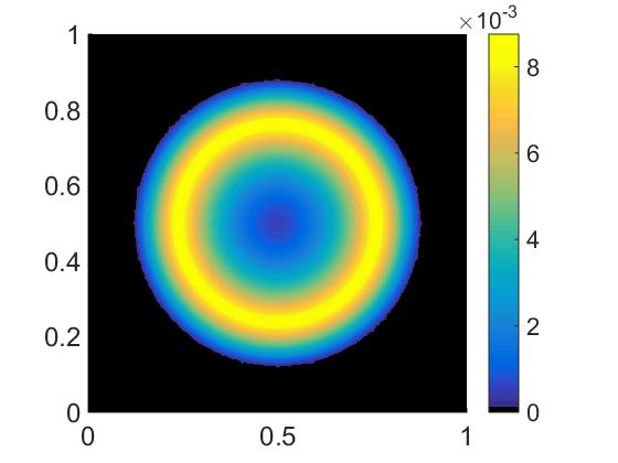
Profile of $G$, $\nu=0.80$	Profile of $G$, $\nu=\nu_{1}^{\star}=0.81$	Profile of $G$, $\nu=0.82$

Figure 8. Topological change of $E_{G}$ near the critical value $\nu_{1}^{\star}=0.81$

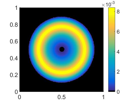
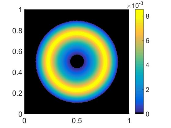
Profil of $F$, $\nu=1.09$	Profil of $F$, $\nu=\nu_{3}^{\star}=1.10$	Profil of $F$, $\nu=1.11$

Figure 9. Topological change of $E_{F}$ near the critical value $\nu_{3}^{\star}=1.10$

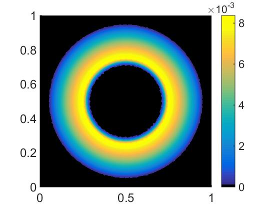
(a) Profile of $F$

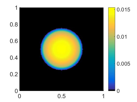
(b) Profile of $G$

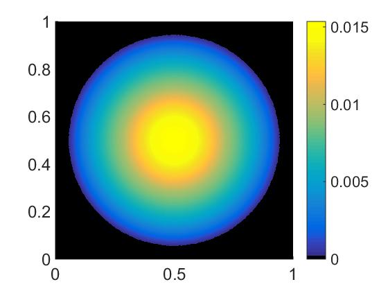
(c) Profile of $F+G$

(d) The fourth configuration

Figure 10. Self-similar profiles for $\nu=2$

(a) Profile of $F$

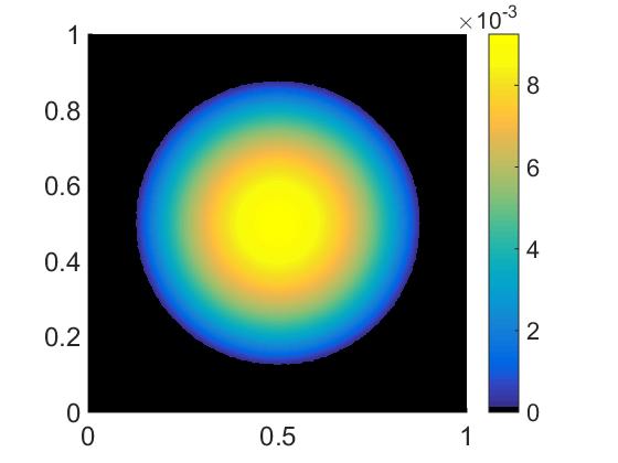
(b) Profile of $G$

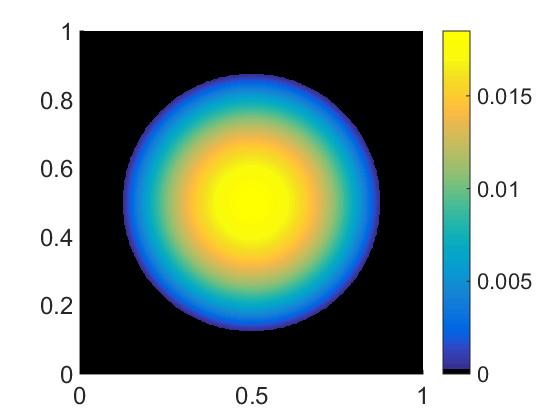
(c) Profile of $F+G$

Figure 11. The critical case $\nu=\nu_{2}^{\star}$ where $E_{F}=E_{G}$.

(a) Profile of $F$ for $\nu=\rho$

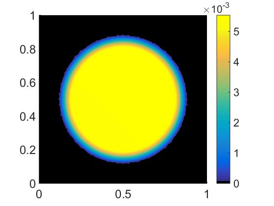
(b) Profile of $G$ for $\nu=\rho$

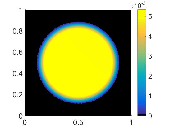
(c) Profile of $F$ for $\nu=1$

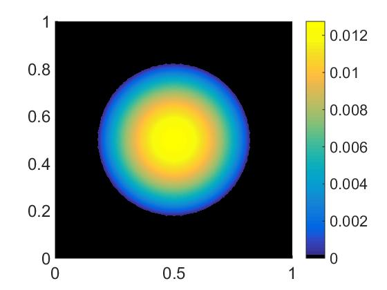
(d) Profile of $G$ for $\nu=1$

Figure 12. The critical values $\nu=\rho$ and $\nu=1$ where the concavity changes on $E_{F}\cap E_{G}$, see (31).

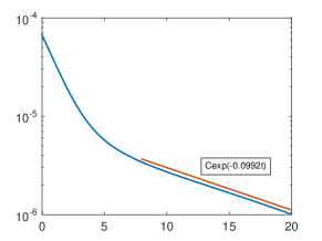
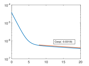
$\nu=0.40$	$\nu=0.90$
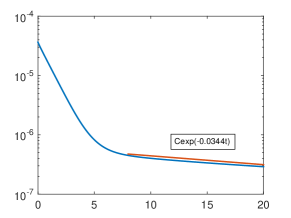
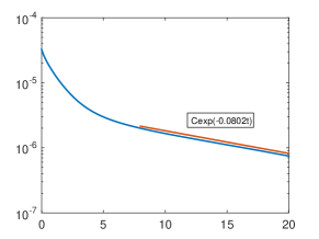
$\nu=0.95$	$\nu=2$

Figure 13. The rate of convergence of the discrete relative energy

Figure 13 suggests that the convergence of the discrete solution to the scheme towards the discrete equilibrium occurs at exponential rate. More precisely we have

(73) $$\mathfrak{E}(f,g|F,G)\leq C\exp(-p(\nu)t),$$

where the rate $p(\nu)$ strongly depends on $\nu$. We plot on Figure 14 the function $\nu\mapsto p(\nu)$ obtained experimentally. At its minimum, the function $p$ is close to 0. This prohibits to conclude to the exponential convergence whatever $\nu\in(0,+\infty)$ and whatever the initial data for the continuous model.

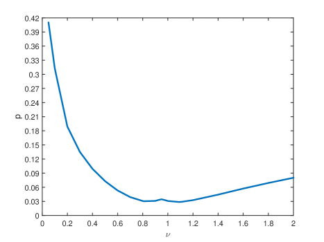
Figure 14. The rate of convergence $p$ in (73) following the values of $\nu$

Appendix A auxiliary results

Lemma A.1.

The embedding $L^{1}(\mathbb{R}^{2})\cap L^{2}(\mathbb{R}^{2})$ in $(W^{1,4}(\mathbb{R}^{2}))^{\prime}$ is continuous.

Proof.

For $g\in L^{1}\cap L^{2}$ and $h\in W^{1,4}$ , one has

$$\left|<g,h>\right| \leq\int_{\{|x|\leq 1\}}|g||h|\mathop{}\!\mathrm{d}x+\int_{\{|x|>1\}}|g||h|\mathop{}\!\mathrm{d}x$$

$$\leq\pi^{1/4}\|g\|_{L^{2}}\|h\|_{L^{4}}+\|g\|_{L^{1}}\|h\|_{L^{\infty}}$$

$$\leq C\left(\|g\|_{L^{2}}+\|g\|_{L^{1}}\right)\|h\|_{W^{1,4}},$$

thanks to the continuous embedding $W^{1,4}(\mathbb{R}^{2})$ in $L^{4}(\mathbb{R}^{2})\cap L^{\infty}(\mathbb{R}^{2}).$ ∎

References

- [1] A. Ait Hammou Oulhaj. A finite volume scheme for a seawater intrusion model with cross-diffusion. In Finite volumes for complex applications VIII—methods and theoretical aspects, volume 199 of Springer Proc. Math. Stat., pages 421–429. Springer, Cham, 2017.
- [2] A. Ait Hammou Oulhaj. Numerical analysis of a finite volume scheme for a seawater intrusion model with cross-diffusion in an unconfined aquifer. Numer. Methods Partial Differential Equations, 2017. to appear, DOI: 10.1002/num.22234.
- [3] L. Ambrosio, N. Gigli, and G. Savaré. Gradient flows in metric spaces and in the space of probability measures. Lectures in Mathematics ETH Zürich. Birkhäuser Verlag, Basel, second edition, 2008.
- [4] L. Arkeryd. On the Boltzmann equation. I: Existence. Arch. Ration. Mech. Anal., 45(1):1–16, 1972.
- [5] A. Arnold, P. Markowich, G. Toscani, and A. Unterreiter. On convex Sobolev inequalities and the rate of convergence to equilibrium for Fokker-Planck type equations. Comm. Partial Differential Equations, 26(1-2):43–100, 2001.
- [6] F. Bolley, I. Gentil, and A. Guillin. Convergence to equilibrium in Wasserstein distance for Fokker-Planck equations. J. Funct. Anal., 263(8):2430–2457, 2012.
- [7] F. Bolley, I. Gentil, and A. Guillin. Uniform convergence to equilibrium for granular media. Arch. Ration. Mech. Anal., 208(2):429–445, 2013.
- [8] E. A. Carlen and S. Ulusoy. An entropy dissipation-entropy estimate for a thin film type equation. Commun. Math. Sci., 3(2):171–178, 2005.
- [9] J. A. Carrillo and G. Toscani. Exponential convergence toward equilibrium for homogeneous Fokker-Planck-type equations. Math. Methods Appl. Sci., 21(13):1269–1286, 1998.
- [10] J. A. Carrillo and G. Toscani. Asymptotic -decay of solutions of the porous medium equation to self-similarity. Indiana Univ. Math. J., 49(1):113–142, 2000.
- [11] C. Choquet, J. Li, and C. Rosier. Global existence for seawater intrusion models: comparison between sharp interface and sharp-diffuse interface approaches. Electron. J. Differential Equations, pages No. 126, 27, 2015.
- [12] L. Desvillettes and K. Fellner. Exponential decay toward equilibrium via entropy methods for reaction-diffusion equations. J. Math. Anal. Appl., 319(1):157–176, 2006.
- [13] L. Desvillettes and K. Fellner. Duality and entropy methods for reversible reaction-diffusion equations with degenerate diffusion. Math. Methods Appl. Sci., 38(16):3432–3443, 2015.
- [14] J. Escher, Ph. Laurençot, and B.-V. Matioc. Existence and stability of weak solutions for a degenerate parabolic system modelling two-phase flows in porous media. Ann. Inst. H. Poincaré Anal. Non Linéaire., 28(4):583–598, 2011.
- [15] J. Escher, A.-V. Matioc, and B.-V. Matioc. Modelling and analysis of the Muskat problem for thin fluid layers. J. Math. Fluid Mech., 14(2):267–277, 2012.
- [16] J. Escher and B.-V. Matioc. Existence and stability of solutions for a strongly coupled system modelling thin fluid films. NoDEA Nonlinear Differential Equations Appl., 20(3):539–555, 2013.
- [17] R. Eymard, T. Gallouët, and R. Herbin. Finite volume methods. In Handbook of numerical analysis, Vol. VII, Handb. Numer. Anal., VII, pages 713–1020. North-Holland, Amsterdam, 2000.
- [18] H. Gajewski and K. Gärtner. On the discretization of van Roosbroeck’s equations with magnetic field. Z. Angew. Math. Mech., 76(5):247–264, 1996.
- [19] H. Gajewski and K. Gröger. On the basic equations for carrier transport in semiconductors. J. Math. Anal. Appl., 113(1):12–35, 1986.
- [20] H. Gajewski and K. Gröger. Semiconductor equations for variable mobilities based on Boltzmann statistics or Fermi-Dirac statistics. Math. Nachr., 140:7–36, 1989.
- [21] A. Glitzky. Exponential decay of the free energy for discretized electro-reaction-diffusion systems. Nonlinearity, 21(9):1989–2009, 2008.
- [22] R. Herbin and F. Hubert. Benchmark on discretization schemes for anisotropic diffusion problems on general grids. In Finite volumes for complex applications V, pages 659–692. ISTE, London, 2008.
- [23] M. Jazar and R. Monneau. Derivation of seawater intrusion models by formal asymptotics. SIAM J. Appl. Math., 74(4):1152–1173, 2014.
- [24] A. Jüngel. Entropy methods for diffusive partial differential equations. SpringerBriefs in Mathematics. Springer, [Cham], 2016.
- [25] Ph. Laurençot and B.-V. Matioc. A gradient flow approach to a thin film approximation of the Muskat problem. Calc. Var. Partial Differential Equations, 47(1-2):319–341, 2013.
- [26] Ph. Laurençot and B.-V. Matioc. A thin film approximation of the Muskat problem with gravity and capillary forces. J. Math. Soc. Japan, 66(4):1043–1071, 2014.
- [27] Ph. Laurençot and B.-V. Matioc. Self-Similarity in a Thin Film Muskat Problem. SIAM J. Math. Anal., 49(4):2790–2842, 2017.
- [28] D. Matthes, R. J. McCann, and G. Savaré. A family of nonlinear fourth order equations of gradient flow type. Comm. Partial Differential Equations, 34(10-12):1352–1397, 2009.
- [29] F. Otto. The geometry of dissipative evolution equations: the porous medium equation. Comm. Partial Differential Equations, 26(1-2):101–174, 2001.
- [30] F. Santambrogio. Optimal Transport for Applied Mathematicians: Calculus of Variations, PDEs, and Modeling. Progress in Nonlinear Differential Equations and Their Applications 87. Birkhäuser Basel, 1 edition, 2015.
- [31] J. Simon. Compact sets in the space . Ann. Mat. Pura Appl. (4), 146:65–96, 1987.
- [32] G. Toscani and C. Villani. On the trend to equilibrium for some dissipative systems with slowly increasing a priori bounds. J. Statist. Phys., 98(5-6):1279–1309, 2000.
- [33] J. L. Vázquez. The porous medium equation. Oxford Mathematical Monographs. The Clarendon Press, Oxford University Press, Oxford, 2007. Mathematical theory.
- [34] A. W. Woods and R. Mason. The dynamics of two-layer gravity-driven flows in permeable rock. J. Fluid Mech., 421:83–114, 2000.
- [35] J. Zinsl and D. Matthes. Exponential convergence to equilibrium in a coupled gradient flow system modeling chemotaxis. Anal. PDE, 8(2):425–466, 2015.