Schwinger-Dyson equation boundary conditions induced by ETC radiative corrections

Abstract

The technicolor (TC) Schwinger-Dyson equations (SDE) should include radiative corrections induced by extended technicolor (ETC) interactions when TC is embedded into a larger theory including also QCD. These radiative corrections couple the different strongly interacting Dyson equations. We discuss how the boundary conditions of the coupled SDE system are modified by these corrections, and verify that the ultraviolet behavior of the self-energies are described by a function that decreases logarithmically with momentum.

I Introduction

The chiral and gauge symmetry breaking in quantum field theories can be promoted by fundamental scalar bosons through the Higgs boson mechanism. If this particle is a composite or an elementary scalar boson is still an open question. Many models have considered the possibility of a light composite Higgs based on effective Higgs potentials as reviewed in Ref.h1 . Nambu and Jona-Lasinio proposed one of the first field theoretical models based on the ideas of superconductivity, where all the most important aspects of chiral symmetry breaking and mass generation, as known nowadays, were explored at length nl . The model of Ref.nl contains only fermions possessing invariance under chiral symmetry, although this invariance is not respected by the vacuum of the theory and the fermions acquire a dynamically generated mass. As a consequence of the chiral symmetry breaking by the vacuum the analysis of the Bethe-Salpeter equation (BSE) shows the presence of Goldstone bosons. These bosons, when the theory is assumed to be the effective theory of strongly interacting hadrons, are associated to the pions. Besides these aspects Nambu and Jona-Lasinio also verified that the theory presents a scalar bound state (the sigma meson), which plays the role of the Higgs boson in their strong interaction model.

In Quantum Chromodynamics (QCD) the same mechanism is observed, where the quarks acquire a dynamically generated mass ($\mu$). This dynamical mass is usually expected to appear as a solution of the SDE for the fermion propagator when the coupling constant is above a certain critical value. The same condition that leads to chiral symmetry breaking is also responsible to generate a bound-state massless pion, and a scalar p-wave state of the BSE, indicating the presence of a scalar state with mass $m_{\sigma}=2\mu$. This scalar meson is the elusive sigma meson pl1 ; pl2 ; pl3 , that is assumed to be the Higgs boson of QCD. This scenario is the accomplishment of Nambu and Jona-Lasinio proposal in the context of renormalizable gauge theories.

The possibility of spontaneous gauge and chiral symmetry breaking promoted by a composite scalar boson in the context of the Standard Model (SM) was formulated in the seventies by Weinberg we and Susskind su . The most popular version of these models was dubbed as technicolor (TC), where new fermions (or technifermions) condensate and may be responsible for the chiral and SM gauge symmetry breaking Rev1 ; Rev2 ; Rev3 . However the phenomenology of these models depend crucially on these new fermions (or technifermions) self-energy. In the early models this self-energy was considered to be given by the result Lane ; ope

$$\Sigma_{TC}(p^{2})\propto\frac{\left\langle{\bar{T}_{f}}T_{f}\right\rangle_{\mu}}{p^{2}}\,\,,$$ (1)

where $\left\langle{\bar{T}_{f}}T_{f}\right\rangle_{\mu}\sim\mu^{3}$ is the TC condensate and $\mu$ is the characteristic TC dynamical mass scale, which is of order of a few hundred GeV, i.e. the order of the SM vacuum expectation value. Unfortunately early technicolor models suffered from problems like flavor changing neutral currents (FCNC) and contributions to the electroweak corrections not compatible with the experimental data Rev1 ; Rev2 ; Rev3 . These problems occur when new extended technicolor interactions (ETC) are introduced in order to provide masses to the standard quarks. Eq.(1) leads to quark masses that vary with the ETC mass scale ($M_{E}$) as $1/M_{E}^{2}$.

A possible way out of this dilemma was proposed by Holdomholdom many years ago, remembering that the self-energy behaves as

$$\Sigma_{TC}(p^{2})\approx\frac{\left\langle{\bar{T}_{f}}T_{f}\right\rangle_{\mu}}{p^{2}}\left(\frac{p}{\mu}\right)^{\gamma_{m}}\,\,$$ (2)

where $\gamma_{m}$ the mass anomalous dimension associated to the fermionic condensate. As can be verified from Eq.(2) a large anomalous dimension leads to a hard asymptotic self-energy (or quasi-conformal technicolor theories) and this may solve the many problems of the SM symmetry breaking promoted by composite bosonswalk2 ; walk3 ; walk4 ; walk5 ; walk6 ; walk7 ; walk8 ; walk9 . Quark masses will be less dependent on the ETC interactions in the case of a hard TC self-energy, leading to a less problematic phenomenology.

There are different ways of obtaining a large $\gamma_{m}$ value in Eq.(2), in what is known as extreme walking (or quasi-conformal) TC theories. (i) It is possible to obtain an almost conformal TC theory when the fermions are in the fundamental representation introducing a large number of TC fermions ($n_{TF}$), leading to an almost zero $\beta$ function and flat asymptotic coupling constant. The cost of such procedure may be a large S parameter peskin1 ; peskin2 , such behavior can also be obtained when the fermions are in larger representations other than the fundamental one sannino1 ; sannino2 ; sannino3 ; or (ii) by inclusion of four-fermion interactionsyama1 ; yama2 ; mira2 ; yama3 ; mira3 ; yama4 .

Most of these studies were performed looking at SDE solutions of the technifermion propagator. In particular, after a work by Takeuchi tak , it became clear that the technifermion self-energy may vary between the behavior of Eq.(1) and the extreme behavior, that in the past was called irregular solution Lane , that is giving by

$$\Sigma_{TC}(p^{2})\approx\mu\left[1+bg^{2}(\mu^{2})\ln\left(p^{2}/\mu^{2}\right)\right]^{-\delta}\,,$$ (3)

where in Eq.(3) $g$ is the TC running coupling constant, $b$ is the coefficient of $g^{3}$ term in the renormalization group $\beta(g)$ function, $\delta=\frac{3c}{16\pi^{2}b}$ , and $c$ is the quadratic Casimir operator given by

$$c=\frac{1}{2}\left[C_{2}(R_{1})+C_{2}(R_{2})-C_{2}(R_{3})\right]\,\,\,,$$

and $C_{2}(R_{i})$, are the Casimir operators for fermions in the representations $R_{1}$ and $R_{2}$ that form a composite boson in the representation $R_{3}$. The behavior of Eq.(3) happens when the theory is totally dominated by a four-fermion interaction, like in the Nambu-Jona-Lasinio model, and it is quite interesting because it may lead to a composite TC scalar boson much lighter than the TC characteristic scale us1 ; us2 ; us4 ; twoscale ; us3 . Eq.(3) leads to quark masses that vary with the ETC mass scale as $[\ln(\mu^{2}/M_{E}^{2})]^{-\delta}$.

It is not surprising that the introduction of a four-fermion interaction may change the ultraviolet SDE behavior. As observed by Cohen and Georgi cg much of the information about chiral symmetry breaking resides into the boundary conditions, and the introduction of new interactions change these conditions. Recently we discussed how the boundary conditions of the anharmonic oscillator representation of the SDE for $SU(N)$ gauge theories are directly related to, and may change, the mass anomalous dimensions us5 . Motivated by this we studied how the introduction of radiative corrections into the SDE may change the self-energy solutions ardn , and verified that when TC is embedded into a larger theory including also QCD, radiative corrections couple the different strongly interacting Dyson equations (TC and QCD) and change completely the ultraviolet behavior of the gap equation solution. The work of Ref.ardn was performed numerically and we just commented, without presenting the details of the calculation, that the effect of the radiative corrections in the coupled equations was similar to a change in the anomalous mass dimension of the theory. The purpose of this work is to show in detail how the coupled TC and QCD have their boundary conditions changed by the ETC radiative corrections, in such a way that the self-energies ultraviolet behavior turn out to be of the form that we may call extreme walking or irregular one, i.e. the behavior of Eq.(3), what may indicate a new way to build TC models as described in Ref.ardn .

This work is organized as follows, in section II we present the TC and QCD coupled SDE system discussed in Ref.ardn , we transform the integral SDE equations into a pair of differential equations, and considering some approximate analytical expressions we recover the numerical result of Ref.ardn , where the quark mass is totally dominated by the irregular solution given by Eq.(3), and in section III we verify how the boundary conditions of the gap equations are changed and are, consequently, responsible by the different asymptotic self-energies behavior. In Section IV we draw our conclusions.

II TC and QCD coupled SDE system by ETC interactions

In Ref.ardn we discussed a coupled SDE system where two strongly interacting theories, TC and QCD, are interconnected by corrections due to ETC and other interactions. These SDE are displayed in Fig.(1). These diagrams appear naturally when QCD and TC are embedded into a larger gauge group, like, for instance, the $SU(5)_{S}$ Farhi-Susskind model far which plays the role of the ETC group. These gap equations may also contain electroweak corrections and, as we are not specifying a model, other possible interactions, which may contribute to the last diagram on the right-hand side of Fig.(1).

In the work of Ref.ardn the SDE equations were solved numerically in a quite simplified approximation, using bare vertices and gauge boson propagators, and verified that the ultraviolet self-energy behaviors of quarks and techniquarks are changed from a soft to a hard behavior, i.e. from a fast to a slow decrease of the self-energy with the momentum. Here we will focus in a detailed analytical approach in order to show that the change in the asymptotic behavior of the self-energies, is a direct consequence of a change of the SDE boundary conditions due to the ETC radiative corrections. In order to do so most of this section is devoted to a detailed discussion of the coupled SDE and to write them in a differential and dimensionless form in order to expose their dependence on the boundary conditions.

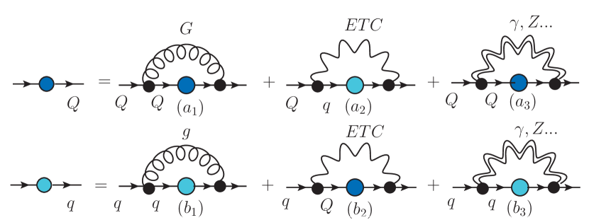
Figure 1: The Schwinger-Dyson equationsardn for QCD(q$\equiv$quark) and TC(Q$\equiv$technifermion) including ETC and electroweak or other corrections($\gamma,Z..$). In the above figure $G\,(g)$ indicate technigluons (gluons) propagators.

The diagrams denoted by $a_{i}$ and $b_{i}$ with $i=1$ in Fig.(1) are respectively the known SDE for techniquarks and quarks. These equations become coupled through the ETC interactions as indicated by the diagrams $a_{2}$ and $b_{2}$. We shall not discuss the effect of diagrams $a_{3}$ and $b_{3}$, which were briefly discussed in Ref.ardn . The TC SDE (diagram $a_{1}$), whose self-energy, coupling constant and respective Casimir operator will be indicated by the index $(1)$, receives a correction (diagram $a_{2}$) due to the quarks self-energy indicated by the index $(2)$ with charge $C_{E}\alpha_{E}$ and gauge boson mass $M_{E}$ related to the ETC group, leading to the following equationardn

$$\Sigma_{1}(p)=\frac{3C_{1}\alpha_{1}}{2\pi^{2}}\int dk^{2}dA\frac{k^{2}\Sigma_{1}(k^{2})}{(p-k)^{2}[k^{2}+\Sigma^{2}_{1}(k^{2})]}+$$

$$\hskip 2.84544pt\frac{3C_{E}\alpha_{E}}{2\pi^{2}}\int dk^{2}dA\frac{k^{2}\Sigma_{2}(k^{2})}{k^{2}+\Sigma^{2}_{2}(k^{2})}\frac{1}{(p-k)^{2}+M^{2}_{E}},$$ (4)

whereas for the quarks self-energy we have a similar equation just changing the index $1\leftrightarrow 2$

$$\Sigma_{2}(p)=\frac{3C_{2}\alpha_{2}}{2\pi^{2}}\int dk^{2}dA\frac{k^{2}\Sigma_{2}(k^{2})}{(p-k)^{2}[k^{2}+\Sigma^{2}_{2}(k^{2})]}+$$

$$\hskip 5.69046pt\frac{3C_{E}\alpha_{E}}{2\pi^{2}}\int dk^{2}dA\frac{k^{2}\Sigma_{1}(k^{2})}{[(p-k)^{2}+M_{E}^{2}]\cdot[k^{2}+\Sigma^{2}_{1}(k^{2})]},$$ (5)

where $dA=d\theta\sin^{2}{\theta}$.

We can easily identify the second term in right-hand side of Eq.(5) as the usual quark mass obtained through TC interaction. With the appropriate QCD values for $C_{2}\alpha_{2}$ and ETC values for $C_{E}\alpha_{E}$ and $M_{E}$ we obtain a solution that is the sum of the dynamical quark mass with its effective “bare mass”. Also Eq.(4) provides the dynamical techniquark mass with a very tiny mass generated by the QCD correction.

The above equations were solved numerically in Ref.ardn . Here they will be transformed into a coupled system of differential equations, therefore we will need to make a few simplifications and the first one is to perform the angular integration using the angle approximationcraig , transforming the following terms as

$$\frac{1}{(p-k)^{2}+M^{2}}=\frac{\pi}{2}\left\{\frac{\theta(p-k)}{p^{2}+M^{2}}+\frac{\theta(k-p)}{k^{2}+M^{2}}\right\},$$ (6)

where in the sequence we may take $M=M_{E}$ or $M=0$.

Continuing with the notation $(1\equiv TC)$ and $(2\equiv QCD)$ we obtain the following form for the system of coupled integral equations

$$f_{1}(x)=\sigma_{1}(x)I^{a}_{1}(x)+\theta_{1}I^{b}_{1}(x)+\zeta_{12}(x)I^{a}_{2}(x)+\eta_{12}I^{b}_{E2}(x)$$

$$f_{2}(x)=\sigma_{2}(x)I^{a}_{2}(x)+\theta_{2}I^{b}_{2}(x)+\zeta_{21}(x)I^{a}_{1}(x)+\eta_{21}I^{b}_{E1}(x).$$

(7)

To arrive at the last expression we introduced the following set of new variables and auxiliary functions

$$p^{2}=M^{2}_{i}x\,\,\,,\,\,\,\Sigma_{i}(p^{2})=M_{i}f_{i}(x)\,\,\,,\,\,\,\omega_{i}=\frac{m^{2}_{i}}{M^{2}_{i}}$$

$$k^{2}=M^{2}_{i}y\,\,\,,\,\,\,\Sigma_{i}(k^{2})=M_{i}f_{i}(y)\,\,\,,\,\,\,\beta_{i}=\frac{M^{2}}{M^{2}_{i}}$$

$$\sigma_{i}(x)=\frac{\theta_{i}}{x+\omega_{i}}\,\,\,,\,\,\,\theta_{i}=\frac{3C_{i}\alpha_{i}}{4\pi}\,\,\,,\,\,\,\theta_{E}=\frac{3C_{E}\alpha_{E}}{4\pi}$$

$$I^{a}_{i}(x)=\int^{x}_{0}dy\frac{yf_{i}(y)}{y+f^{2}_{i}(y)}\,\,\,,\,\,\,g_{i}(x)=\frac{xf_{i}(x)}{x+f^{2}_{i}(x)}$$

$$I^{b}_{i}(x)=\int^{\frac{\Lambda^{2}}{M^{2}_{i}}}_{x}dy\frac{yf_{i}(y)}{y+f^{2}_{i}(y)}\frac{1}{y+\omega_{i}}$$

$$I^{b}_{Ei}(x)=\int^{\frac{\Lambda^{2}}{M^{2}_{i}}}_{x}dy\frac{yf_{i}(y)}{y+f^{2}_{i}(y)}\frac{1}{y+\beta_{i}}$$

$$\zeta_{ij}(x)=\frac{\theta_{E}}{x+\beta_{i}}\left(\frac{M_{j}}{M_{i}}\right)^{3}\,\,\,,\,\,\,\eta_{ij}=\theta_{E}\left(\frac{M_{j}}{M_{i}}\right).$$ (8)

In the above expressions $M=M_{E}$, $i,j=1(2)$ denote the contributions of TC(QCD) to the coupled gap equation. Note that $M_{1}=\mu_{{}_{1}}$, and $M_{2}=\mu_{{}_{2}}$, where $\mu_{i}$ correspond respectively to the dynamical TC and QCD fermionic mass scales, $m_{i}$ represents technigluons(or gluons) dynamical mass scale mg1 ; mg2 ; mg3 ; mg4 , which were not considered in Ref.ardn .

In order to transform the coupled system of integral equations described by Eq.(7) into a system of coupled differential equations for $f_{i}(x)$ we also introduce new functions $\delta_{1}(x)$ and $\delta_{2}(x)$ , where

$$\delta_{1}(x)=\frac{\zeta^{\prime}_{12}(x)\left(f^{\prime}_{2}(x)+\frac{\eta_{21}g_{1}(x)}{x+\beta_{1}}-\zeta_{21}(x)g_{1}(x)\right)}{\zeta^{\prime}_{12}(x)\zeta^{\prime}_{21}(x)-\sigma^{\prime}_{2}(x)\sigma^{\prime}_{1}(x)}$$

$$-\frac{\sigma^{\prime}_{2}(x)\left(f^{\prime}_{1}(x)+\frac{\eta_{12}g_{2}(x)}{x+\beta_{2}}-\zeta_{12}(x)g_{2}(x)\right)}{\zeta^{\prime}_{12}(x)\zeta^{\prime}_{21}(x)-\sigma^{\prime}_{2}(x)\sigma^{\prime}_{1}(x)}$$ (9)

$$\delta_{2}(x)=\frac{\zeta^{\prime}_{21}(x)\left(f^{\prime}_{1}(x)+\frac{\eta_{12}g_{2}(x)}{x+\beta_{2}}-\zeta_{12}(x)g_{2}(x)\right)}{\zeta^{\prime}_{12}(x)\zeta^{\prime}_{21}(x)-\sigma^{\prime}_{2}(x)\sigma^{\prime}_{1}(x)}$$

$$-\frac{\sigma^{\prime}_{1}(x)\left(f^{\prime}_{2}(x)+\frac{\eta_{21}g_{1}(x)}{x+\beta_{1}}-\zeta_{21}(x)g_{1}(x)\right)}{\zeta^{\prime}_{12}(x)\zeta^{\prime}_{21}(x)-\sigma^{\prime}_{2}(x)\sigma^{\prime}_{1}(x)},$$

(10)

in such a way that now we can write

$$f^{\prime\prime}_{1}(x)+\frac{\eta_{12}g^{\prime}_{2}(x)}{x+\beta_{2}}+\frac{\zeta_{12}(x)g_{2}(x)}{x+\beta_{1}}=\frac{\eta_{12}g_{2}(x)}{(x+\beta_{2})^{2}}$$

$$\hskip 27.5992pt+\,\zeta_{12}(x)g^{\prime}_{2}(x)+\sigma^{\prime\prime}_{1}(x)\delta_{1}(x)+\sigma^{\prime}_{1}(x)\delta^{\prime}_{1}(x)$$

$$\hskip 27.5992pt+\frac{}{}\zeta^{\prime\prime}_{12}(x)\delta_{2}(x)+\zeta^{\prime}_{12}(x)\delta^{\prime}_{2}(x)$$

(11)

$$f^{\prime\prime}_{2}(x)+\frac{\eta_{21}g^{\prime}_{1}(x)}{x+\beta_{1}}+\frac{\zeta_{21}(x)g_{1}(x)}{x+\beta_{2}}=\frac{\eta_{21}g_{1}(x)}{(x+\beta_{1})^{2}}$$

$$\hskip 27.5992pt+\,\zeta_{21}(x)g^{\prime}_{1}(x)+\sigma^{\prime\prime}_{2}(x)\delta_{2}(x)+\sigma^{\prime}_{2}(x)\delta^{\prime}_{2}(x)$$

$$\hskip 27.5992pt+\frac{}{}\zeta^{\prime\prime}_{21}(x)\delta_{1}(x)+\zeta^{\prime}_{21}(x)\delta^{\prime}_{1}(x).$$

(12)

It is an exercise the verification that Eqs.(11) and (12) can be solved by a linear combination of two solutions. One that is called regular, where the self-energies behave at large momenta as $1/x$, and another one, called irregular, where the self-energies decrease as $[\ln x]^{-\epsilon}$, where $\epsilon$ is a function of the quantities $b$ and $c$. Only when the boundary conditions are applied to these equations the actual self-energy ultraviolet behavior is selected. This is the central point of the work of Ref.ardn and the one that we present here: The ETC radiative corrections cause the selection of the irregular solution and not the one behaving as $1/x$!

How the ETC corrections will change the SDE boundary conditions and the solution behavior will be shown in the next section. However, in a very naive approximation for Eq.(5) we can show in the sequence that quark masses vary logarithmically with the ETC mass scale (i.e. $M_{E}$), which is a consequence of a TC self-energy with a logarithmic ultraviolet (UV) behavior ardn . As can be seen from Eq.(5) the full quark mass ($m_{q}$) is a sum of the dynamical mass generated within QCD, with the one generated through TC mediated by the ETC interaction. Using Eq.(6) and approximating $m_{q}$ by $\Sigma_{2}(0)$ we can simplify Eq.(5) and obtain

$$m_{q}\approx\Sigma_{2}(0)\approx\frac{3C_{2}\alpha_{2}}{4\pi}\int_{0}^{\Lambda}dk^{2}\frac{\Sigma_{2}(k)}{k^{2}+\Sigma^{2}_{2}(k)}$$

$$\hskip 17.07182pt+\frac{3C_{E}\alpha_{E}}{4\pi}\int_{0}^{\Lambda}dk^{2}\frac{\Sigma_{1}(k)}{k^{2}+\Sigma^{2}_{1}(k)}\frac{1}{k^{2}+M^{2}_{E}}$$

$$\hskip 17.07182pt+\frac{3C_{2}\alpha_{2}}{4\pi}\frac{1}{M^{2}_{E}}\int_{0}^{\Lambda}dk^{2}\frac{\Sigma_{2}(k)}{k^{2}+\Sigma^{2}_{2}(k)}$$

$$\hskip 17.07182pt+\frac{3C_{E}\alpha_{E}}{4\pi}\frac{1}{2M^{2}_{E}}\int_{0}^{\Lambda}dk^{2}\frac{\Sigma_{1}(k)}{k^{2}+\Sigma^{2}_{1}(k)}$$ (13)

This is an oversimplified equation compared to Eq.(5) and gives $m_{q}$ as a function of $M_{E}$. We can now input the solutions of Eqs.(11) and (12) into Eq.(13) and solve it up to the convergence. The convergence is obtained only with the solution that has a logarithmic UV behavior.

Even within the simplified approach shown above it is possible to compare the calculation of Eq.(13) with the full numerical result obtained in Ref.ardn . Therefore, assuming $\Lambda=500$TeV, $M_{1}=\mu_{1}=1$TeV, $M_{2}=\mu_{2}=0.3$GeV, $C_{1}\alpha_{1}=6$ and $C_{2}\alpha_{2}=1.16$ values such that isolated techniquark and quark masses were equal respectively to $\mu_{1}$ and $\mu_{2}$ as in Ref.ardn , and $C_{E}\alpha_{E}=0.032$, we plot $m_{q}$ as a function of $M_{E}$ in Fig.(2).

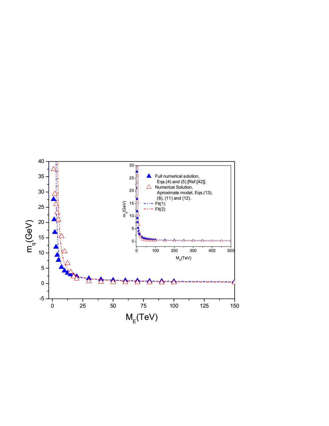
Figure 2: Behavior of $m_{q}$ as a function of $M_{E}$ obtained from Eq.(13) using the solutions of Eqs.(12) and (11) (red curve(${\color[rgb]{1,0,0}\Delta}$)). The blue curve(${\color[rgb]{0,0,1}\blacktriangle}$) corresponds to the result obtained in ardn . The dot-dash lines represents the Fit(1)(blue dot-dash line) and Fit(2) (Red dot-dash line) , the parameters are described in the text.

The blue curve(${\color[rgb]{0,0,1}\blacktriangle}$) corresponds to the result obtained in ardn , while the red curve(${\color[rgb]{1,0,0}\Delta}$) is the numerical one obtained with Eqs.(11) , (12) and (13). The dot-dash lines represent the fit

$$m_{q}^{fit}\propto a_{1}[ln(M^{2}_{E}/M^{2}_{2})]^{-a_{2}}\,,$$ (14)

where for the Fit(1) (blue dot-dash) we obtain , $a_{1}=203.92$GeV and $a_{2}=2.53$ with $R^{2}=0.99$ and for Fit(2) (Red dot-dash) , $a_{1}=1620$GeV and $a_{2}=3.6$ with $R^{2}=0.93$. The behavior exhibited by the curves in Red depicted in Fig.(2) are very similar to the one obtained in the Ref.ardn . The small discrepancy between these different results can be credited to the angle approximation and the simple approximation made here to calculate $m_{q}$. However, the main point is that in TC models as proposed here, the dependence of quark masses on the ETC mass scale is definitively logarithmic and not a power law, which is a consequence of quark masses computed with a techniquark self-energy as the one shown in Eq.(3). In the next section we show that both self-energies (techniquarks and quarks) have the same asymptotic behavior induced by the ETC interaction.

III UV boundary conditions induced by ETC radiative corrections

In order to determine the boundary conditions of our SDE coupled system we can differentiate Eqs.(7) obtaining

$$f^{\prime}_{1}(x)=\sigma^{\prime}_{1}(x)I^{a}_{1}(x)+\zeta^{\prime}_{12}(x)I^{a}_{2}(x)$$

$$f^{\prime}_{2}(x)=\sigma^{\prime}_{2}(x)I^{a}_{2}(x)+\zeta^{\prime}_{21}(x)I^{a}_{1}(x),$$

(15)

from these expressions and reconsidering Eq.(7) in the asymptotic UV limit, such that $(\frac{\Lambda^{2}}{M^{2}_{i}}=\frac{M^{2}_{E}}{M^{2}_{i}}>>1)$ we end up the following set of coupled equations

$$f_{1}(x)+xf^{\prime}_{1}(x)=\zeta_{12}(x)I^{a}_{2}(x)$$

$$f_{2}(x)+xf^{\prime}_{2}(x)=\zeta_{21}(x)I^{a}_{1}(x)$$ (16)

which correspond to the UV boundary conditions that should be satisfied by Eqs.(11) and (12). Reconsidering the definitions of variables and auxiliary functions described in Eq.(8) the above expressions above lead to

$$\left[\Sigma_{1}(p^{2})+p^{2}\Sigma^{\prime}_{1}(p^{2})\right]_{p^{2}\rightarrow\infty}=m_{2},$$

$$\left[\Sigma_{2}(p^{2})+p^{2}\Sigma^{\prime}_{2}(p^{2})\right]_{p^{2}\rightarrow\infty}=m_{1},$$

(17)

where

$$m_{1(2)}=\frac{3C_{E}\alpha_{E}}{4\pi}\int dk^{2}\frac{k^{2}\Sigma_{1(2)}(k^{2})}{k^{2}+\Sigma^{2}_{1(2)}(k^{2})}\frac{1}{k^{2}+M^{2}_{E}}.$$ (18)

It is easy to recognize that Eqs.(17) when $\alpha_{E}=0$, i.e. when the equations are decoupled, we have

$$\left[\Sigma_{1}(p^{2})+p^{2}\Sigma^{\prime}_{1}(p^{2})\right]_{p^{2}\rightarrow\infty}=0,$$

$$\left[\Sigma_{2}(p^{2})+p^{2}\Sigma^{\prime}_{2}(p^{2})\right]_{p^{2}\rightarrow\infty}=0,$$

(19)

and it has long been known that the asymptotic behavior of $\Sigma_{1}(p^{2})$ (or $\Sigma_{2}(p^{2})$) is described byLane

$$\Sigma_{1(2)}(p^{2}\rightarrow\infty)\propto\frac{\mu^{3}_{1(2)}}{p^{2}}$$ (20)

which lead to quark masses $m_{q}\approx\Sigma_{2}(0)$ of order

$$m_{q}\approx C_{E}\alpha_{E}\frac{M^{3}_{1}}{M_{E}^{2}},$$ (21)

which is at the origin of all known problems of TC models Rev1 .

When we turn on the ETC interaction, i.e. $\alpha_{E}\neq 0$, the equations (17) differ only by their infrared (IR) boundary conditions, which are usually set as $\Sigma_{1}(0)=M_{1}$ and $\Sigma_{2}(0)=M_{2}$. If, apart only from different numerical scales, we set $\Sigma_{1}(0)=\Sigma_{2}(0)\equiv M$ eqs.(17) will give

$$\left[\Sigma_{1}(p^{2})+p^{2}\Sigma^{\prime}_{1}(p^{2})\right]_{p^{2}\rightarrow\infty}=M(p^{2}\rightarrow\infty),$$

$$\left[\Sigma_{2}(p^{2})+p^{2}\Sigma^{\prime}_{2}(p^{2})\right]_{p^{2}\rightarrow\infty}=M(p^{2}\rightarrow\infty),$$

(22)

where $M(p^{2}\rightarrow\infty)\propto M[\ln p^{2}/M^{2}]^{-\epsilon}$ and there is no doubt that $\Sigma_{1}(p^{2})$ and $\Sigma_{2}(p^{2})$ have exactly the same IR and UV behavior, and when $M_{1}\neq M_{2}$ they just differ numerically in the IR but have the same functional expression. This is a confirmation of the statement in Ref.ardn that in the scenario proposed there the TC and QCD self-energies have exactly the same UV asymptotic behavior.

If we do not assume the same IR conditions for both self-energies we can again verify that $\Sigma_{1}(p^{2})$ and $\Sigma_{2}(p^{2})$ have formally the same UV behavior. Initially we can observe that in the deep Euclidean region we have

$$f_{i}(x\rightarrow\infty)\approx\frac{\theta_{i}}{x}\delta_{i}(x),$$ (23)

but in the same limit and after some algebra we can see that $\delta_{1}(x)$ and $\delta_{2}(x)$ have also the same expression apart from a constant, therefore

$$\left.f_{1}(x)\right|_{x\rightarrow\infty}\propto\left.f_{2}(x)\right|_{x\rightarrow\infty},$$ (24)

indicating that both self-energies decrease equally in the UV region.

The main difference in the UV boundary conditions in the decoupled and coupled SDE, assuming that $\Sigma_{1}(p^{2})$ and $\Sigma_{2}(p^{2})$ have the same formal expression and both can be substituted by an expression $\Sigma(p^{2})$, is an effective mass term

$$m=\frac{3C_{E}\alpha_{E}}{4\pi}\int dk^{2}\frac{k^{2}\Sigma(k^{2})}{k^{2}+\Sigma^{2}(k^{2})}\frac{1}{k^{2}+M^{2}_{E}},$$ (25)

and this term is going to act like a “bare” mass, whose effect is to generate a logarithmically decreasing self-energy for quarks and techniquarks.

IV Conclusions

In the Ref.ardn we have given evidences that radiative corrections to TC(QCD) change the UV technifermion(quark) self-energy behavior. This happens when TC and QCD are embedded into an unified theory as in the Farhi-Susskind model (or an ETC model). In this work we verify that in these cases the radiative corrections that couple the different strongly interacting Dyson equations induce new boundary conditions for the gap equations and change the UV behavior compared to the isolated equations.

We transformed the coupled TC and QCD coupled equations into a pair of differential equations. These two equations may have as a solution a linear combination of the known regular and irregular self-energies. When these solutions are applied to a quite simplified mass equation (Eq.(13)), derived from the original gap equation, we verified that quark masses vary logarithmically with the ETC scale, what is a consequence of a TC self-energy that also decreases logarithmically with the momentum. This is a simple confirmation of the more complete numerical calculation of Ref.ardn . The simple quark mass (Eq.(13)) acts as a constraint for the differential equations solution, appearing as an effective mass boundary condition.

In Section III we discussed how the ETC interaction induce a change into the boundary conditions, and this change is equivalent to the addition of an effective bare mass to the gap equation, which leads naturally to a self-energy logarithmically decreasing with the momentum. Moreover, as stated in Ref.ardn , we also discussed that both self-energies have the same formal expression and, along with the discussion of that same reference, may lead to a new way to build TC models.

References

- (1) B. Bellazzini, C. Csáki and J. Serra, Eur. Phys. J. C 74, 2766 (2014).
- (2) Y. Nambu and G. Jona-Lasinio, Phys. Rev. 122, 345 (1961).
- (3) R. Delbourgo and M. D. Scadron, Phys. Rev. Lett. 48, 379 (1982).
- (4) N. A. Tornqvist and M. Roos, Phys. Rev. Lett. 76, 1575 (1996).
- (5) N. A. Tornqvist and A. D. Polosa, Nucl. Phys. A 692, 259 (2001).
- (6) N. A. Tornqvist and A. D. Polosa, Frascati Phys. Ser. 20, 385 (2000).
- (7) S. Weinberg, Phys. Rev. D 19 1277 (1979).
- (8) L. Susskind, Phys. Rev. D 20, 2619 (1979).
- (9) C. T. Hill and E. H. Simmons, Phys. Rept. 381, 235 (2003) [Erratum-ibid. 390, 553 (2004)].
- (10) F. Sannino, hep-ph/0911.0931, Lectures presented at the 49th Cracow School of Theoretical Physics. Conformal Dynamics for TeV Physics and Cosmology, Cracow, Nov , 2009; Acta Phys. Polon.. B 40, 3533 (2009); Int. J. Mod. Phys. A 20, 6133 (2005).
- (11) K. Lane, Technicolor 2000 , Lectures at the LNF Spring School in Nuclear, Subnuclear and Astroparticle Physics, Frascati (Rome), Italy, May 15-20, 2000.
- (12) K. Lane, Phys. Rev. D 10, 2605 (1974).
- (13) H. D. Politzer, Nucl. Phys. B 117, 397 (1976).
- (14) B. Holdom, Phys. Rev. D 24, 1441 (1981).
- (15) B. Holdom, Phys. Lett. B 150, 301 (1985).
- (16) T. Appelquist, D. Karabali e L. C. R. Wijewardhana, Phys. Rev. Lett. 57, 957 (1986).
- (17) T. Appelquist and L. C. R. Wijewardhana, Phys. Rev. D 36, 568 (1987).
- (18) T. Appelquist, M. Piai, and R. Shrock, Phys. Rev. D69, 015002 (2004).
- (19) T. Appelquist, M. Piai and R. Shrock, Phys. Lett. B 593 , 175 (2004).
- (20) T. Appelquist and R. Shrock, Phys. Rev. Lett. 90, 201801-1 (2003).
- (21) T. Appelquist and R. Shrock, Phys. Lett. B 548 , 204 (2002).
- (22) M. Kurachi, R. Shrock and K. Yamawaki, Phys. Rev. D 76, 035003 (2007).
- (23) M. E. Peskin and T. Takeuchi, Phys. Rev. Lett. 65, 964 (1990).
- (24) M. E. Peskin and T. Takeuchi, Phys. Rev. D 46, 381 (1992).
- (25) F. Sannino and K. Tuominen, Phys. Rev. D 71, 051901 (2005).
- (26) R. Foadi, M. T. Frandsen, T. A. Ryttov and F. Sannino, Phys. Rev. D 76, 055005 (2007).
- (27) T. A. Ryttov and F. Sannino, Phys. Rev. D 78, 115010 (2008).
- (28) V. A. Miransky and K. Yamawaki, Mod. Phys. Lett. A 4, 129 (1989).
- (29) K.-I. Kondo, H. Mino and K. Yamawaki, Phys. Rev. D39, 2430 (1989).
- (30) V. A. Miransky, T. Nonoyama and K. Yamawaki, Mod. Phys. Lett. A4, 1409 (1989).
- (31) T. Nonoyama, T. B. Suzuki and K. Yamawaki, Prog. Theor. Phys.81, 1238 (1989).
- (32) V. A. Miransky, M. Tanabashi and K. Yamawaki, Phys. Lett. B221, 177 (1989).
- (33) K.-I. Kondo, M. Tanabashi and K. Yamawaki, Mod. Phys. Lett. A8, 2859 (1993).
- (34) T. Takeuchi, Phys. Rev. D 40, 2697 (1989).
- (35) A. Doff, A. A. Natale and P. S. Rodrigues da Silva, Phys. Rev. D 77, 075012 (2008).
- (36) A. Doff, A. A. Natale and P. S. Rodrigues da Silva, Phys. Rev. D 80, 055005 (2009).
- (37) A. Doff, E. G. S. Luna and A. A. Natale, Phys. Rev. D 88, 055008 (2013).
- (38) A. Doff and A. A. Natale, Phys. Lett. B 748, 55 (2015).
- (39) A. Doff and A. A. Natale, Int. J. Mod. Phys. A 31, 1650024 (2016).
- (40) A. Cohen and H. Georgi, Nucl. Phys. B 314, 7 (1989).
- (41) A. Doff and A. A. Natale, Phys. Lett. B 771, 392 (2017).
- (42) A. C. Aguilar , A. Doff and A. A. Natale, hep-ph/1802.03206.
- (43) E. Farhi and L. Susskind, Phys. Rev. D 20, 3404 (1979).
- (44) Craig D. Robertz and Bruce H. J. McKellar, Phys. Rev. D 41, 672 (1990).
- (45) J. M. Cornwall, Phys. Rev. D 26, 1453 (1982).
- (46) A. C. Aguilar, D. Binosi and J. Papavassiliou, Phys. Rev. D 78, 025010 (2008).
- (47) A. C. Aguilar and J. Papavassiliou, Phys. Rev. D 83, 014013 (2011).
- (48) A. Doff, F. A. Machado and A. A. Natale, Annals of Physics 327, 1030 (2012).