Experimental Implementation of Generalized Transitionless Quantum Driving
Abstract
It is known that high intensity fields are usually required to implement shortcuts to adiabaticity via Transitionless Quantum Driving (TQD). Here, we show that this requirement can be relaxed by exploiting the gauge freedom of generalized TQD, which is expressed in terms of an arbitrary phase when mimicking the adiabatic evolution. We experimentally investigate the performance of generalized TQD in comparison with both traditional TQD and adiabatic dynamics. By using a 171Yb+ trapped ion hyperfine qubit, we implement a Landau-Zener adiabatic Hamiltonian and its (traditional and generalized) TQD counterparts. We show that the generalized theory provides energy-optimal Hamiltonians for TQD, with no additional fields required. In addition, the optimal TQD Hamiltonian for the Landau-Zener model is investigated under dephasing. Even using less intense fields, optimal TQD exhibits fidelities that are more robust against a decohering environment, with performance superior than that provided by the adiabatic dynamics.
I Introduction
Transitionless Quantum Driving (TQD) Demirplak:03 ; Demirplak:05 ; Berry:09 is a useful technique to mimic adiabatic quantum tasks at finite time. It has been applied for speeding up adiabaticity in several applications, such as quantum gate Hamiltonians Santos:15 ; Santos:16 ; Coulamy:16 , heat engines in quantum thermodynamics Adolfo:16 , quantum information processing Marcela:14 ; Xia:16 ; Chen:10 , among others (e.g., Refs. Stefanatos:14 ; Lu:14 ; Deffner:16 ; XiaPRA:14 ; Song:16 ; Adolfo:13 ; Saberi:14 ; An:16 ; Zhang:16 ). To perform TQD we need to design a counter-diabatic Hamiltonian , given by , where denotes the set of instantaneous eigenstates of the original adiabatic Hamiltonian and the dot symbol denotes time derivative. The Hamiltonian enables us to cancel any transition between two different eigenstates of . It should be added to the original Hamiltonian to yield the shortcut to adiabaticity Hamiltonian, which is given by .
In general, the Hamiltonian allows us to exactly mimic an adiabatic dynamics at arbitrary finite time, so that, by starting at a given initial eigenstate of , the evolved state is given by , where is the adiabatic phase Berry:84 . However, there are several applications where we do not need to exactly mimic an adiabatic phase , as long as the system is kept in an eigenstate of the Hamiltonian Santos:15 ; Santos:16 ; Coulamy:16 ; Adolfo:16 ; Marcela:14 ; Xia:16 ; Chen:10 ; Stefanatos:14 ; Lu:14 ; Deffner:16 ; XiaPRA:14 ; Song:16 ; Adolfo:13 ; Saberi:14 ; An:16 ; Zhang:16 ; Liang:16 ; Yi:17 ; Ramanathan:16 . Thus, it has been proposed a generalized approach for TQD, where we consider that the phases that accompany the dynamics can be taken as arbitrary Torrontegui:13 ; Santos:18-b . Therefore, differently from traditional TQD, where the dynamics is driven by , in generalized TQD the dynamics is driven by a generalized shortcut to adiabaticity Hamiltonian written as Torrontegui:13 ; Santos:18-b ; Chen:11
| (1) |
where are arbitrary real parameters. In this case, the evolved generalized state is written as , with arbitrary . It is worth highlighting that (1) shows that we can mimic an adiabatic task even when our physical system does not allow for a direct implementation of the adiabatic Hamiltonian. In addition, as it was discussed in Santos:18-b , we can also take advantage of these generalized phases to simplify the Hamiltonian , possibly even removing in certain situations its dependence on time.
Concerning robustness against decoherence, some experimental and theoretical studies of TQD in different experimental architectures have shown promising features, such as in nitrogen-vacancy setups Liang:16 , trapped ions An:16 , atoms in cavities Xia:16 ; Yi:17 , nuclear magnetic resonance (NMR) Ramanathan:16 , and optomechanics Zhang:16 . These works consider the traditional approach for shortcuts to adiabaticity, where the adiabatic phase is taken when mimicking the adiabatic dynamics. As theoretically found out in Ref. Santos:18-b , generalized TQD may provide much better resistance against decoherence depending on the time window designed to run the quantum process.
In this paper, we report the first experimental implementation aiming at verifying the advantage of generalized TQD with respect to its adiabatic and traditional TQD counterparts. More specifically, we implement the energetically optimal version of generalized TQD in a two-level system realizing the Landau-Zener model. Our physical system is composed of a single 171Yb+ ion confined in a Paul trap, where the system dynamics is driven by the Landau-Zener Hamiltonian. It has previously been shown that the traditional TQD method requires high intensity fields Santos:15 ; Santos:16 ; Coulamy:16 ; Campbell-Deffner:17 ; Abah:17 . As we shall see, generalized TQD theory requires much less intense fields while capable of providing better fidelities. In particular, for the dynamics considered here, while traditional TQD requires additional fields, the generalized theory allows us to mimic an adiabatic dynamics without additional fields. Moreover, the dynamics under dephasing shows the superiority of the generalized TQD approach, with higher fidelities with less expenditure of energy resources.
II Optimal TQD for the Landau-Zener Hamiltonian
We consider a quantum bit (qubit) undergoing an adiabatic dynamics governed by the Landau-Zener Hamiltonian, which reads , with a detuning between the microwave frequency and the atom transition level; is the Rabi frequency and is the normalized time. The system is initialized in the ground state of and adiabatically evolves to , where , with a time-dependent dimensionless parameter that satisfies the boundary conditions and . Traditional TQD mimics the above dynamics through the Hamiltonian , where , with the function chosen as for obtaining a time-independent counter-diabatic Hamiltonian (see, e.g., Ref. Santos:18-b ).
However, in this scenario, we still need to implement a time-dependent contribution due to the adiabatic Hamiltonian . On the other hand, if we adopt generalized TQD, we can implement the transitionless dynamics through the simplest time-dependent Hamiltonian given by . As in Ref. Santos:18-b , the energetically optimal Hamiltonian above is obtained by choosing the phases in (1) through a geometric contribution, such as , which implies here in . The turns out to be implemented by a flat -pulse, whose robustness has been investigated for fast population transfer in Ref. X-Jing:13 .
III Experimental setup
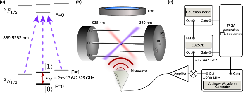
We now demonstrate the experimental implementation of generalized TQD, with a single ion trapped in a six needles Paul trap, which is shown in Fig. 1(b). We encode a qubit into two hyperfine energy levels of the ground state, which is denoted by and , as shown in Fig. 1(a). Applying a 6.40 G static magnetic field, the clock transition frequency between and is 12.642 825 GHz.
In a configuration of a frequency mixing scheme with an arbitrary waveform generator (AWG), we can coherently drive the hyperfine qubit. The scheme is shown in Fig. 1(c), a 12.442 GHz microwave is mixed with the AWG signals around 200 MHz, to generate the operating waveform. The AWG waveform is programmed to control and , for implementing the target Hamiltonian. In addition, in order to mimic the two level system interacting with an environment, we introduced a Gaussian noise frequency modulation of the 12.442 GHz microwave, which can be viewed as a dephasing channel. It is a remarkable fact that the dephasing channel is premium and highly controlled. After Doppler cooling of the trapped ion, we apply a standard optical pumping process to initialize the qubit into the state with 99.9% efficiency. After the qubit operation with microwave sequence, a florescence detection method is used to measure the population of the the state olmschenk_2007 . The florescence of the trapped ion is collected by an optical lens with a numerical aperture of NA = 0.4, then pass an optical bandpass filter and a pinhole, and is finally detected by a PMT with 20% quantum efficiency. Within 300 detection time, the target state preparation and measurement fidelity is measured as 99.4% blume-kohout_2017 .
III.1 Microwave fields and energy resources
In our experiment we used both resonant and off-resonant microwaves fields to implement adiabatic and TQD dynamics. The adiabatic dynamics was performed by using a non-resonant microwave, where the time-dependent effective Rabi frequency is given by . To drive the system by using the traditional TQD, we use an independent microwave to simulate the counter-diabatic term . This additional field is a resonant microwave (), whose Rabi frequency can be obtained as . On the other hand, different from traditional TQD Hamiltonian, the optimal dynamics driven by could be implemented using a single resonant microwave with Rabi frequency , where we have turned-off the non-resonant field used for simulate .
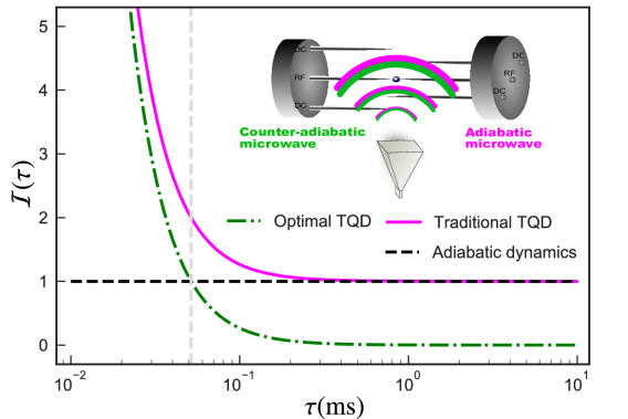
In order to quantify the energy resources employed in the quantum evolution, we study the intensity of the fields used to perform the adiabatic dynamics as well as traditional and optimal TQD. The field intensity is associated with the Rabi frequency through the relation , where is a constant that depends on the microwave amplifier. Considering the whole evolution time, we can define the average intensity field as . So, for the adiabatic dynamics we have , for the optimal TQD we get , and for the traditional TQD we find , since the traditional TQD field is composed by both the adiabatic and the optimal TQD contributions. For convenience, we disregard the constant by taking relative field intensities expressed in unities of the adiabatic intensity . Then, we define and , and adopt the normalization . These field intensities are plotted in Fig 2, with an schematic representation of each dynamics indicated in the inset. As we can see from Fig. 2, we can define a value for the total evolution time for which the intensity fields for implementing optimal TQD becomes less intense than the adiabatic intensity. By computing we get ms and we represent this boundary using a vertical line in Fig. 2. Notice that, after , the shortcut to adiabaticity defined by the optimal TQD can be implemented by spending less energy resources, as measured by the field intensity, than the adiabatic approach.
An alternative approach to compute the energy cost is to estimate the energy scale through the time-average Hamiltonian norm Santos:15 ; Santos:16 ; Santos:18-b ; Coulamy:16 ; Nathan:14 . In this direction, let us consider a quantum dynamics driven by a time-dependent Hamiltonian, with energy cost defined as . For the specific case of the Landau-Zener model, this method takes into account not only the external field intensities but also the detuning . Indeed, exerts influence over the energy gap spectrum, which may justify its accounting in some scenarios, such as adiabatic quantum computation. From this definition, we can show that , for every . Moreover, there is again a boundary value for which we get for , as originally predicted in Ref. Santos:18-b . Here, we obtain ms. Thus, we can see that an analysis from energy scale of the Hamiltonian provides a (qualitatively) equivalent result to the intensity ields analysis. In both cases, it is shown that, by specifically designing a suitable time window, shortcuts to adiabaticity can be implemented in such a way to accelerate physical processes while saving energy resources.
IV Robustness against decoherence
Owing to the long coherence time of the 171Yb+ trapped ion hyperfine qubit, the decoherence effects for the timescale adopted in the experimental setup is negligible. Therefore, to simulate the interaction of the Landau-Zener system with an environment, we introduce a Gaussian noise capable of implementing a dephasing channel where the system will be driven by a Lindblad equation given by , where is the dephasing rate. To quantify the robustness of the protocols, we use the fidelity , which is related to the Bures length Bures:69 , with being solution of Lindblad equation and .
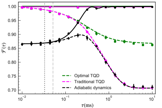
We start by disregarding decoherence and implementing each protocol for several choices of msms. The results are shown in Fig. 3. Since the maximum total evolution time is ms (i.e., times shorter than the coherence time of the qubit), the dynamics can be considered as approximately unitary. The continuum lines in Fig. 3 show the fidelities under a unitary dynamics for each protocol and the corresponding experimental data points. The black curve shows that the adiabatic behavior is achieved for long total evolution time ms, with computed from , where is the gap between fundamental and excited energy levels Sarandy:04 . Notice that, for fast evolutions (ms), both optimal and traditional TQD provide a high fidelity protocol, while adiabatic dynamics fails. Naturally, this high performance is accompanied by costly fields used for implementing the TQD protocols, as previously shown in Fig. 2. On the other hand, it is important to highlight that for total evolution time , where the optimal TQD field is smaller than both adiabatic and traditional TQD ones, the high performance of optimal TQD is kept. By looking now at the effect of the dephasing channel, we can see that optimal TQD exhibits the highest robustness for every , with its advantage increasing as increases. For fast evolution times, this high performance is again associated with costly fields in comparison with the adiabatic fields. However, for large evolution times, while the traditional TQD fidelity converges to adiabatic fidelity, the fidelity behavior of optimal TQD is much better than both adiabatic dynamics and traditional TQD, with less energy resources spent in the process. This is a remarkable result, since we can achieve both better fidelities with less energy fields involved, where we get even when .
V Conclusion
In this paper we have experimentally investigated the performance of shortcuts to adiabaticity by exploiting the gauge freedom as we fix the phase accompanying the evolution dynamics. In particular, we have focused on the optimal TQD, comparing it with its associated adiabatic dynamics and traditional TQD counterparts. Our main results are: i) The optimal version of generalized TQD has been shown to be a useful protocol for obtaining the optimal shortcut to adiabaticity. While adiabatic and traditional TQD require time-dependent quantum control, optimal TQD can be experimentally realized by using time-independent fields. In addition, the necessity of auxiliary fields in traditional TQD is not a requirement for implementing TQD via its optimal version. ii) Optimal TQD is an energetically optimal protocol of shortcut to adiabaticity. By considering the average intensity fields as a measure of energy cost for implementing the protocols discussed here, we were able to show that the optimal version of generalized TQD may be energetically less demanding. This result is kept also for alternatives definitions of energy cost, e.g. taking into account the detuning contribution. iii) By simulating an environment-system coupling associated with the dephasing channel, we have shown that optimal TQD can be more robust than the adiabatic dynamics and the traditional TQD while at the same time spending less energy resources for a finite time range. In addition, we were able to to mimic the adiabatic behavior through time-independent Hamiltonian, showing that the optimal theory works. Once the Landau-Zener Hamiltonian can be implemented in others physical systems, e.g. nuclear magnetic resonance Nielsen:Book and two-level systems driven by a chirped field Demirplak:03 , it is reasonable to think that the results obtained here can be also realized in other experimental architectures. Moreover, inverse engineering protocols are an interesting candidate to implement fast and robust elementary quantum gates for quantum computing Santos:15 ; Santos:16 ; Coulamy:16 ; Santos:18-a . Thus, an experimental investigation of these protocols can be a promising direction as a future research, as can the robustness of optimal TQD against others classes of errors (as it has been done for traditional TQD in Ref. Ruschhaupt:12 ).
VI Funding Information
This work was supported by the National Key Research and Development Program of China (No. 2017YFA0304100), National Natural Science Foundation of China (Nos. 61327901, 61490711,11774335, 11734015, 11474268, 11374288, 11304305,11404319), Anhui Initiative in Quantum Information Technologies (AHY070000), Key Research Program of Frontier Sciences, CAS (No. QYZDY-SSWSLH003), the National Program for Support of Top-notch Young Professionals (Grant No. BB2470000005), the Fundamental Research Funds for the Central Universities (WK2470000026). A.C.S. is supported by CNPq-Brazil. M.S.S. is supported by CNPq-Brazil (No. 303070/2016-1), FAPERJ (No. 203036/2016), and the Brazilian National Institute for Science and Technology of Quantum Information (INCT-IQ).
References
- (1) M. Demirplak and S. A. Rice, J. Phys. Chem. A 107, 9937 (2003).
- (2) M. Demirplak and S. A. Rice, J. Phys. Chem. B 109, 6838 (2005).
- (3) M. Berry, J. Phys. A: Math. Theor. 42, 365303 (2009).
- (4) A. C. Santos and M. S. Sarandy, Sci. Rep. 5, 15775 (2015).
- (5) A. C. Santos, R. D. Silva, and M. S. Sarandy, Phys. Rev. A 93, 012311 (2016).
- (6) I. B. Coulamy, A. C. Santos, I. Hen, and M. S. Sarandy, Frontiers in ICT 3, 19 (2016).
- (7) M. Beau, J. Jaramillo, and A. del Campo, Entropy 18, 168 (2016).
- (8) M. Herrera, M. S. Sarandy, E. I. Duzzioni, and R. M. Serra, Phys. Rev. A 89, 022323 (2014).
- (9) Z. Chen, Y. Chen, Y. Xia, J. Song, and B. Huang, Sci. Rep. 6, 22202 (2016).
- (10) X. Chen, I. Lizuain, A. Ruschhaupt, D. Guéry-Odelin, and J. G. Muga, Phys. Rev. Lett. 105, 123003 (2010).
- (11) D. Stefanatos, Phys. Rev. A 90, 023811 (2014).
- (12) M. Lu, Y. Xia, L.-T. Shen, J. Song, and N. B. An, Phys. Rev. A 89, 012326 (2014).
- (13) S. Deffner, New J. Phys. 18, 012001 (2016).
- (14) Y.-H. Chen, Y. Xia, Q.-Q. Chen, and J. Song, Phys. Rev. A 89, 033856 (2014).
- (15) X.-K. Song, H. Zhang, Q. Ai, J. Qiu, and F.-G. Deng, New J. Phys. 18, 023001 (2016).
- (16) A. del Campo, Phys. Rev. Lett. 111, 100502 (2013).
- (17) H. Saberi, T. c. v. Opatrný, K. Mølmer, and A. del Campo, Phys. Rev. A 90, 060301 (2014).
- (18) S. An, D. Lv, A. Del Campo, and K. Kim, Nat. Commun. 7, 12999 (2016).
- (19) H. Zhang, X.-K. Song, Q. Ai, M. Zhang, and F.-G. Deng, arXiv:1610.09938 (2016).
- (20) M. V. Berry, Proc. R. Soc. A 392, 45 (1984).
- (21) Z.-T. Liang et al., Phys. Rev. A 93, 040305 (2016).
- (22) S. L. Wu, X. L. Huang, H. Li, and X. X. Yi, Phys. Rev. A 96, 042104 (2017).
- (23) J. Vandermause and C. Ramanathan, Phys. Rev. A 93, 052329 (2016).
- (24) E. Torrontegui et al., Adv. At. Mol. Opt. Phys 62, 117 (2013).
- (25) A. C. Santos and M. S. Sarandy, J. Phys. A: Math. Theor. 51, 025301 (2018).
- (26) X. Chen, E. Torrontegui, and J. G. Muga, Phys. Rev. A 83, 062116 (2011).
- (27) S. Campbell and S. Deffner, Phys. Rev. Lett. 118, 100601 (2017).
- (28) O. Abah and E. Lutz, Europhys. Lett. (EPL) 118, 40005 (2017).
- (29) X.-J. Lu et al., Phys. Rev. A 88, 033406 (2013).
- (30) S. Olmschenk et al., Physical Review A 76, 052314 (2007).
- (31) R. Blume-Kohout et al., Nature Communications 8, 14485 (2017).
- (32) M. Kieferová and N. Wiebe, New J. Phys. 16, 123034 (2014).
- (33) D. Bures, Trans. Am. Math. Soc. 135, 199 (1969).
- (34) M. S. Sarandy, L.-A. Wu, and D. A. Lidar, Quantum Information Processing 3, 331 (2004).
- (35) M. A. Nielsen and I. L. Chuang, Quantum Computation and Quantum Information: 10th Anniversary Edition, 10th ed. (Cambridge University Press, New York, NY, USA, 2011).
- (36) A. C. Santos, J. Phys. B: At. Mol. Opt. Phys. 51, 015501 (2018).
- (37) A. Ruschhaupt, X. Chen, D. Alonso, and J. Muga, New J. Phys. 14, 093040 (2012).