Effective anisotropy due to the surface of magnetic nanoparticles

Abstract

Analytical solution has been found for the second-order effective anisotropy of magnetic nanoparticles of a cubic shape due to the surface anisotropy (SA) of the Néel type. Similarly to the spherical particles, for the simple cubic lattice the grand-diagonal directions $\left(\pm 1,\pm 1,\pm 1\right)$ are favored by the effective cubic anisotropy but the effect is twice as strong. Uniaxial core anisotropy and applied magnetic field cause screening of perturbations from the surface at the distance of the domain-wall width and reduce the effect of SA near the energy minima. However, screening disappears near the uniaxial energy barrier, and the uniform barrier state of larger particles may become unstable. For these effects the analytical solution is obtained as well, and the limits of the additive formula with the uniaxial and effective cubic anisotropies for the particle are established. Thermally-activated magnetization-switching rates have been computed by the pulse-noise technique for the stochastic Landau-Lifshitz equation for a system of spins.

I Introduction

In magnetic nanoparticles, a significant fraction of atoms belongs to the surface, and their magnetic properties such as exchange and anisotropy can be strongly modified. With successes in synthesis of magnetic particles of a controlled shape, it has become feasible to investigate the effects of the surface on the magnetic properties numerically and even analytically. One of the important ingredients is surface anisotropy (SA) proposed by Néel Néel (1954) and modeled microscopically by Victora and MacLaren Victora and MacLaren (1993). SA arises due to missing neighbors for the surface spins and breaking the symmetry of their crystal field and it must be much stronger than a typical crystallographic anisotropy in the particle’s core. However, there is still not much information on the SA in different materials Chuang et al. (1994); Respaud et al. (1998); Chen et al. (1999). The most common manifestation of the SA is decreasing of the effective anisotropy of magnetic films with the thickness $d$ as $K_{\mathrm{eff}}=K_{V}+K_{S}/d$, where $K_{V}$ and $K_{S}$ are volume and surface contributions Chuang et al. (1994); Bødker et al. (1994); Respaud et al. (1998); Chen et al. (1999). It was found that atomic steps on surfaces strongly contribute into the effective anisotropy Chuang et al. (1994); Moroni et al. (2003).

In small magnetic clusters, individual spins are tightly bound together by the exchange interaction, and they form an effective rigid giant spin with an effective anisotropy dependent on the surface. In particular, the Néel SA (NSA) was used to model the effective anisotropy of Co nanoclusters of the form of truncated octahedrons Jamet et al. (2001, 2004). In this case, contributions of different faces and edges partially cancel each other, leading to a significantly reduced result. For totally symmetric shapes such as spherical and cubic, the cancellation of the SA for the rigid cluster’s spin is complete.

However, individual spins can deviate from collinearity for stronger SA and larger particles Dimitrov and Wysin (1994a, b); Dimian and Kachkachi (2002); Kachkachi and Dimian (2002). Examples of strong noncollinearity are “throttled” and “hedgehog” spin configurations Dimitrov and Wysin (1994a, b); Labaye et al. (2002); Berger et al. (2008). Small non-collinearity can be treated perturbatively Garanin and Kachkachi (2003); Usov and Grebenshchikov (2008), that results into the second-order effective anisotropy Garanin and Kachkachi (2003) $K_{\mathrm{eff}}\sim D_{S}^{2}/J$, where $D_{S}$ is the SA and $J$ is the exchange. For particles with simple cubic (sc) lattice and spherical shape it was found that the effective second-order anisotropy has a cubic symmetry with the lowest energy along the grand diagonals $\left(\pm 1,\pm 1,\pm 1\right)$ of the sc lattice, where the deviations from collinearity and the resulting energy gain are maximal. The result scales with the particle’s volume as perturbations from the surface penetrate into the particle’s core. Thus in experiments, the second order effective anisotropy cannot be easily identified with the surface. If the particle’s size becomes too large, deviations from the collinearity become so strong that the perturbation theory becomes invalid. For magnetic particles with shapes close to symmetric, the first- and second-order effective anisotropies can coexist and compete with each other Yanes et al. (2007).

As the SA must be much stronger than the core anisotropy, both first-and second-order surface terms can compete with the latter. In the simplest additive approximation, for symmetric shapes one can just add the uniaxial core anisotropy and the cubic second-order surface anisotropy that leads to complicated energy landscapes Kachkachi and Bonet (2006); Yanes et al. (2007). In Refs. Yanes et al. (2007); Yanes and Chubykalo-Fesenko (2009) it was shown that for the face-centered (fcc) lattice the sign of the second-order surface anisotropy is inverted, so that the directions $\left(\pm 1,0,0\right)$ etc., have the lowest energy. Different temperature dependences of the core and effective surface anisotropies may cause reorientation transitions on temperature, as was shown in Ref. Yanes et al. (2010) using the constrained Monte Carlo method Asselin et al. (2010). Additive effective anisotropy of magnetic particles affects their dynamic properties such as magnetic resonance Kachkachi and Schmool (2007) and thermally-activated switching Déjardin et al. (2008); Coffey et al. (2009); Vernay et al. (2014).

As it was mentioned in Ref. Garanin and Kachkachi (2003), in the presence of the uniaxial core anisotropy $D$, the effect of the surface will be screened at the distance of the domain-wall width $\delta=a\sqrt{J/(2D)}$ from the surfaces, $a$ being the lattice spacing. Thus the effect of the surfaces should be reduced for the particle’s sizes $L\gtrsim\delta$. Another effect is the mixing term in the effective anisotropy arising from both core and surface anisotropies and having another symmetry Yanes et al. (2007).

All analytical and numerical investigations mentioned above were performed on spherical particles, plus ellipsoidal and truncated octahedron shapes in Refs. Yanes et al. (2007); Yanes and Chubykalo-Fesenko (2009). Analytical solution for the deviations from collinearity in spherical particles uses the Green’s function for the internal Neumann problem for the Laplace equation in a sphere. Studying the screening requires solving the Helmholtz equation for which the Green’s function in a sphere is unknown. For this reason, screening was investigated only perturbatively in the $L/\delta\ll 1$ limit in Ref. Yanes et al. (2007). A closed-form expression for the Green’s function of Laplace and Helmholts equations for cubes and parallelepipeds is unknown. This hampered the investigation of these shapes, although they are no less important than spherical and ellipsoidal. For instance, recently Fe nanocubes have been synthesized Zhao et al. (2016).

Fortunately, for the cubic shape there is an exact analytical solution that is direct and not using Green’s functions. This solution is much simpler than that for the spherical shape and it allows an extension for the case of screening by the core anisotropy and by the applied field. This is the subject of this paper. In particular, it will be shown that screening is active near the energy minima but becomes “anti0screening” closer to the barriers, that leads to stronger noncollinearities and eventually to the destruction of the quasi-uniform barrier states.

The plan of the paper is the following. In Sec. II the model of classical spins with surface anisotropy is introduced and the expression for the first-order effective particle’s surface anisotropy is obtained for parallelepipeds. In Sec. III the method of constrained energy minimization needed to deal with deviations from spin collinearity in the particle is reviewed and further developed in comparison to previous publications. This method is needed for both numerical and analytical work. In Sec. IV the numerical implementation of the constrained energy minimization is discussed. Sec. V contains the analytical solution for the second-order effective anisotropy for the cubic particle with sc lattice in the absence of the core anisotropy and maghetic field. Sec. VI shows the numerical results obtained by the constrained energy minimization and their comparizon with the analytical results. In Sec. VII a more general analytical solution in the presence of the uniaxial core anisotropy and the magnetic field is obtained and the effects of screening are investigated. Sec. VIII presents the results for the thermally-activated magnetization switching of the cubic particle considered as a many-spin system.

II The model

The magnetic particle will be described by the classical spin Hamiltonian

$$\mathcal{H}=-D\sum_{i\in\mathrm{core}}s_{zi}^{2}+\sum_{i\in\mathrm{surface}}\mathcal{H}_{SA,i}-\mathbf{h}\cdot\sum_{i}\mathbf{s}_{i}-\frac{1}{2}\sum_{ij}J_{ij}\mathbf{s}_{i}\cdot\mathbf{s}_{j},$$ (1)

where $\mathbf{h}\equiv\mu_{0}\mathbf{H}$ is the magnetic field in the energy units, $\mathcal{H}_{SA}$ is the surface anisotropy, $J_{ij}$ is the exchange with the coupling $J$ between the neighboring spins on a sc lattice, $D$ is the core uniaxial-anisotropy constant, and $|\mathbf{s}_{i}|=1$. The Néel’s surface anisotropy is given by Néel (1954); Victora and MacLaren (1993)

$${\cal H}_{SA,i}=\frac{1}{2}D_{S}\sum_{j\in nn}\left(\mathbf{s}_{i}\cdot{\bf u}_{ij}\right)^{2},$$ (2)

where $\mathbf{u}_{ij}$ is the unit vector connecting the surface site $i$ to its nearest neighbor on site $j$. This anisotropy arises due to missing nearest neighbors for the surface spins. In particular, for the simple cubic lattice and $xy$ surfaces (those perpendicular to $z$ axis), the Néel anisotropy becomes ${\cal H}_{SA,i}=-\frac{1}{2}D_{S}s_{iz}^{2}$ . This means that for $D_{S}>0$ the spins tend to align perpendicularly to the surface, while for $D_{S}<0$ the surface spins tend to align parallel to the surface. In a parallelepiped-shaped particle, the Néel anisotropy on the edges along $z$ axis becomes ${\cal H}_{SA,i}=-\frac{1}{2}D_{S}\left(s_{ix}^{2}+s_{iy}^{2}\right)$ or, equivalently, ${\cal H}_{SA,i}=\frac{1}{2}D_{S}s{}_{iz}^{2}$. Thus for $D_{S}>0$ the $z$-edge spins tend to align perpendicularly to $z$ axis. The Néel anisotropy vanishes at the corners and in the core of the particle.

Spins in particles small enough are tightly bound together by the exchange and forming an effective giant spin. For a parallelepiped-shaped particle of the size $N_{z}\times N_{y}\times N_{z}=\mathcal{N}$ the effective Hamiltonian

$$\mathcal{H}_{\mathrm{eff}}=-\mathcal{N}_{\mathrm{core}}Ds_{z}^{2}+\mathcal{H}_{SA}^{(1)}-\mathcal{N}\mathbf{h}\cdot\mathbf{s},$$ (3)

where $\mathcal{N}_{\mathrm{core}}=\left(N_{z}-2\right)\times\left(N_{y}-2\right)\times\left(N_{z}-2\right)$ and $\mathcal{H}_{SA}^{(1)}$ is the sum of contributions from 6 surfaces and 12 edges

$$\mathcal{H}_{SA}^{(1)} = -D_{S}\left[\left(N_{y}N_{z}-4\right)s_{x}^{2}+\left(N_{z}N_{x}-4\right)s_{y}^{2}\right.$$ (4)

$$\qquad\qquad+\left.\left(N_{x}N_{y}-4\right)s_{z}^{2}\right].$$

This expression vanishes for $N_{x}=N_{y}=N_{z}=2$ since in this case there are neither faces nor edges, only corners. For $D_{S}>0,$ the lowest-energy direction is perpendicular to the biggest faces. For $D_{S}<0,$ the lowest-energy direction is perpendicular to the smallest faces. For $N_{x}=N_{y}\equiv N_{\bot}$ the model becomes uniaxial

$$\mathcal{H}_{SA}^{(1)}=-D_{S}N_{\bot}\left(N_{\bot}-N_{z}\right)s_{z}^{2}.$$ (5)

The first-order effective anisotropy due to the surface scales with the surface, thus for large particle sizes $L$ it becomes small as $1/L$ in comparison to the contribution of the core anisotropy.

III Deviations from collinearity and constrained energy minimization

For the particle of a cubic shape, $\mathcal{H}_{SA}^{(1)}=0$ but there still is a second-order contribution $\mathcal{H}_{SA}^{(2)}\sim D_{S}^{2}/J$ due to deviation from collinearity generated by the SA. These deviations depend on the orientation $\boldsymbol{\nu}$ of the particle’s magnetization $\mathbf{m}$, where

$$\mathbf{m}\equiv\frac{1}{\mathcal{N}}\sum_{i}\mathbf{s}_{i},\qquad\boldsymbol{\nu}\equiv\frac{\mathbf{m}}{m}.$$ (6)

Larger deviations correspond to a larger adjustment energy gain, thus the corresponding directions of $\mathbf{m}$ have lower energy Garanin and Kachkachi (2003). Deviations from the collinearity are introduced via the formula

$$\mathbf{s}_{i}=\boldsymbol{\nu}\sqrt{1-\boldsymbol{\psi}_{i}^{2}}+\boldsymbol{\psi}_{i}\cong\boldsymbol{\nu}\left(1-\frac{1}{2}\boldsymbol{\psi}_{i}^{2}\right)+\boldsymbol{\psi}_{i},\qquad\sum_{i}\boldsymbol{\psi}_{i}=0.$$ (7)

Below $\boldsymbol{\psi}_{i}$ will be calculated within the linear approximation.

To define the particle’s energy for different $\mathbf{m}$ directions $\boldsymbol{\nu}$, one has to constrain the latter. This can be done by using the method of Lagrange multipliers Garanin and Kachkachi (2003); Kachkachi and Bonet (2006); Yanes et al. (2007); Paz et al. (2008) in which one minimizes the function

$$\mathcal{F}\equiv\mathcal{H}-\mathcal{N}\boldsymbol{\lambda}\cdot\left(\boldsymbol{\nu}-\boldsymbol{\nu}_{0}\right),$$ (8)

where $\boldsymbol{\nu}_{0}$ is the preset direction, $|\boldsymbol{\nu}_{0}|=1$. The constrained equilibrium solution satisfies the equations

$$\mathbf{s}_{i}\times\frac{\partial\mathcal{F}}{\partial\mathbf{s}_{i}}=0,\qquad\frac{\partial\mathcal{F}}{\partial\boldsymbol{\lambda}}=-\mathcal{N}\left(\boldsymbol{\nu}-\boldsymbol{\nu}_{0}\right)=0.$$ (9)

From the second equation follows $\boldsymbol{\nu}=\boldsymbol{\nu}_{0}$. In the first equation

$$-\frac{\partial\mathcal{F}}{\partial\mathbf{s}_{i}}=\mathbf{h}_{\mathrm{eff},i}+\mathbf{h}_{\lambda},\qquad\mathbf{h}_{\mathrm{eff},i}\equiv-\frac{\partial\mathcal{H}}{\partial\mathbf{s}_{i}}$$ (10)

and the constraint field is uniform and given by

$$\mathbf{h}_{\lambda}\equiv\mathcal{N}\frac{\partial\left(\boldsymbol{\lambda}\cdot\boldsymbol{\nu}\right)}{\partial\mathbf{s}_{i}}=\frac{1}{m}\left[\boldsymbol{\lambda}-\boldsymbol{\nu}\cdot\left(\boldsymbol{\nu}\cdot\boldsymbol{\lambda}\right)\right].$$ (11)

Note that $\mathbf{h}_{\lambda}$ is perpendicular to $\mathbf{m}$ since it constrains only its direction $\boldsymbol{\nu}$, leaving its magnitude $m$ free to change.

Analytically, the constraint field can be found at zero order in $\boldsymbol{\psi}_{i}$, considering the rigid particle’s spin and averaging the effective field over the particle to get the contribution of the surface. Thus the first of equations (9) becomes

$$\boldsymbol{\nu}\times\left(\mathbf{\bar{h}}_{\mathrm{eff}}+\mathbf{h}_{\lambda}\right)=0,$$ (12)

where from Eq. (3) one obtains

$$\mathbf{\bar{h}}_{\mathrm{eff}}=\mathbf{h}+2\tilde{D}\nu_{z}\mathbf{e}_{z}+\mathbf{h}_{SA},\qquad\tilde{D}\equiv\frac{\mathcal{N}_{\mathrm{core}}}{\mathcal{N}}D$$ (13)

and

$$\mathbf{h}_{SA}\equiv-\frac{1}{\mathcal{N}}\frac{\partial\mathcal{H}_{SA}^{(1)}\left(\boldsymbol{\nu}\right)}{\partial\boldsymbol{\nu}}.$$ (14)

In particular, for $N_{x}=N_{y}\equiv N_{\bot}$ one obtains

$$\mathbf{h}_{SA}=2D_{S}\frac{N_{\bot}-N_{z}}{N_{\bot}N_{z}}s_{s}\mathbf{e}_{z}.$$ (15)

Since $\mathbf{h}_{\lambda}$ is perpendicular to $\boldsymbol{\nu}$, the solution of Eq. (12) is

$$\mathbf{h}_{\lambda}=-\mathbf{\bar{h}}_{\mathrm{eff}}+\boldsymbol{\nu}\left(\boldsymbol{\nu}\cdot\mathbf{\bar{h}}_{\mathrm{eff}}\right).$$ (16)

IV Numerical methods

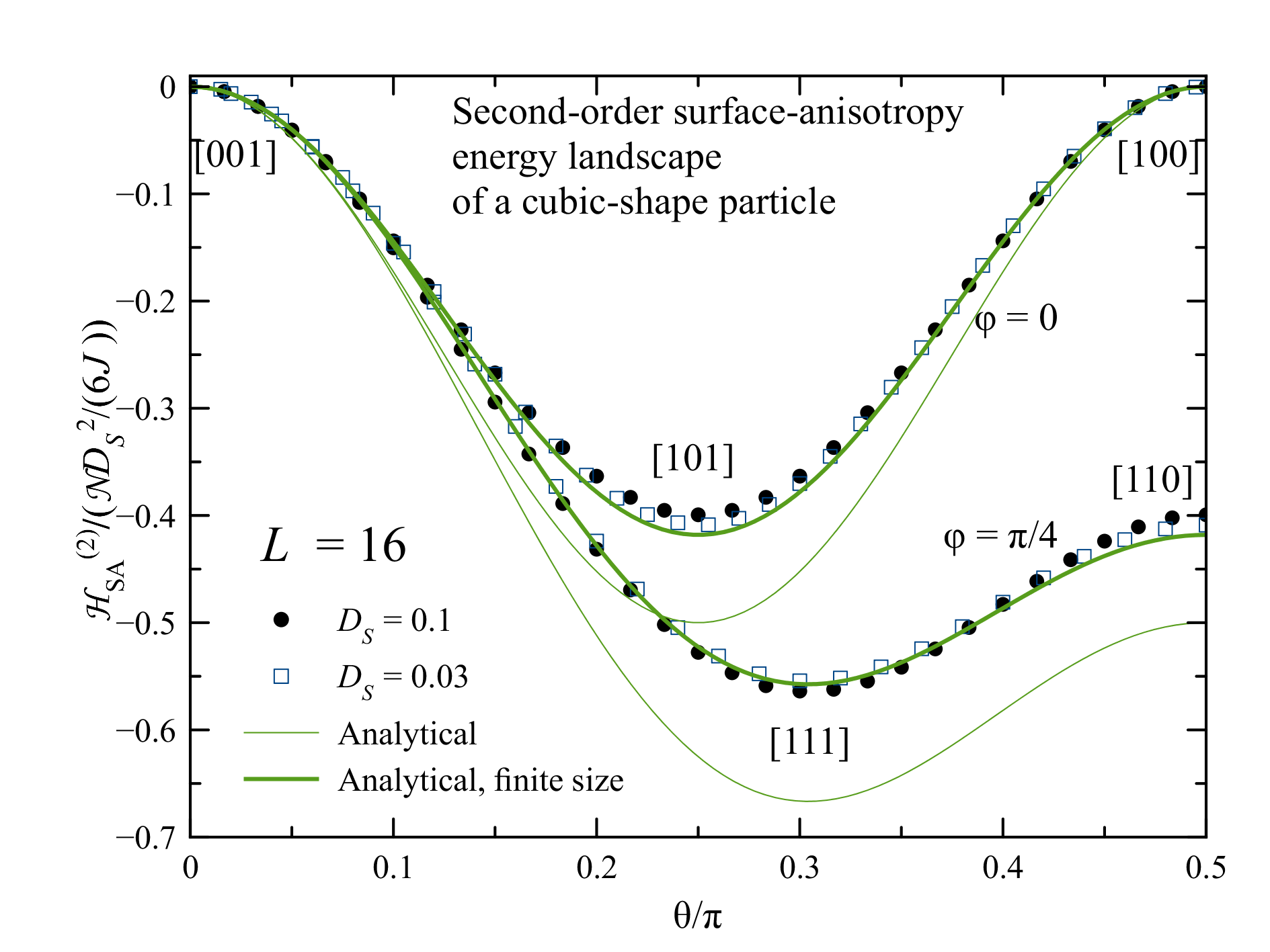
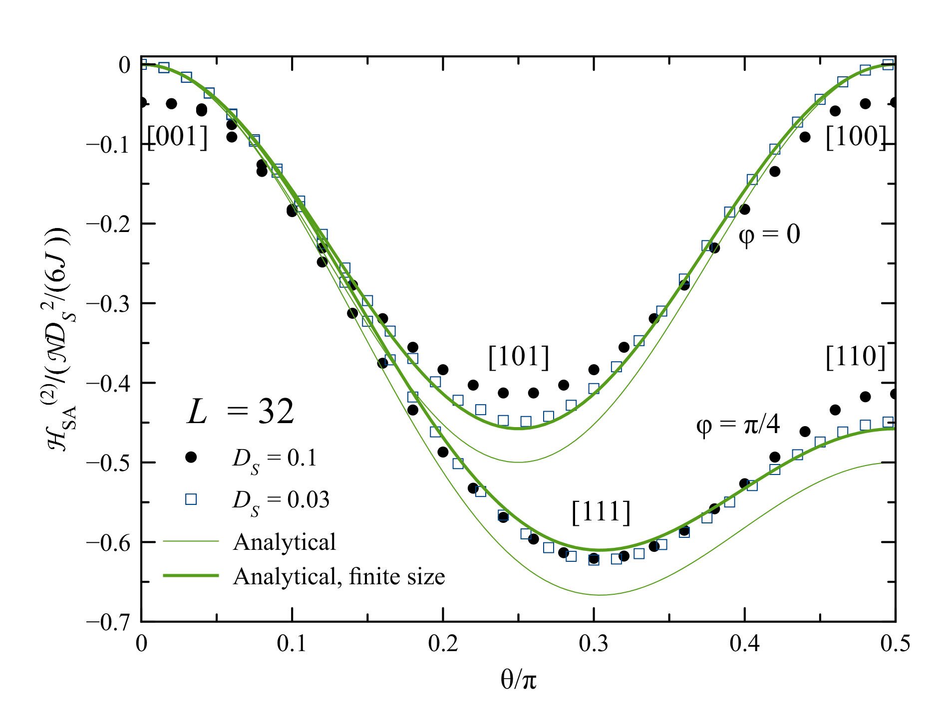
Figure 1: Energy landscape for the cubic particle with the surface anisotropy: Numerical and analytical results for the particle sizes $L=16$, 32 and the SA strenghts $D_{S}=0.1,$ 0.03. “Analytical” curves use Eq. (34) while “Analytical, finite size” curves use Eq. (34) with the additional factor $(1-0.7/L)^{4}$.

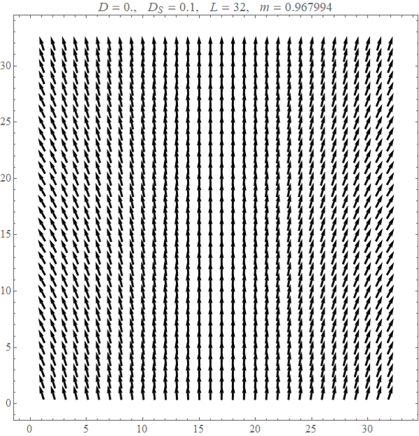
Figure 2: Spin structures in a cubic particle of the size $L=32$ for $D_{S}=0.1$, scans through middle of the particle. Upper panel: particle’s magnetization direction $\left(1,1,0\right)$ etc. Spins slightly canted to lower the system’s energy in accordance with the analytical solution, Eq. (27). Lower panel: particle’s magnetization direction $\left(0,0,1\right)$. Spins slightly turned toward the directions perpendicular to the right and left surfaces as the result of the instability of the collinear state (for $L=16$ spins are still strictly collinear).

One practical method of numerically solving Eq. (9) is the method of relaxation in which the evolution equations

$$\mathbf{\dot{s}}_{i} = -\alpha\mathbf{s}_{i}\times\left[\mathbf{s}_{i}\times\left(\mathbf{h}_{\mathrm{eff},i}+\mathbf{h}_{\lambda}\right)\right]$$

$$\dot{\boldsymbol{\lambda}} = \frac{\alpha_{\lambda}}{\mathcal{N}}\frac{\partial\mathcal{F}}{\partial\boldsymbol{\lambda}}=-\alpha_{\lambda}\left(\boldsymbol{\nu}-\boldsymbol{\nu}_{0}\right)$$ (17)

with relaxation constants $\alpha$ and $\alpha_{\lambda}$ are solved Garanin and Kachkachi (2003); Kachkachi and Bonet (2006); Yanes et al. (2007). A faster method is a combination of the field alignment and overrelaxation used in Refs. Garanin et al. (2013a, b); Proctor et al. (2014) for finding local energy minima in magnetic systems with quenched randomness. In this method, all spins $\mathbf{s}_{i}$ are updated consequtively by the field alignment $\mathbf{s}_{i,\mathrm{new}}=\mathbf{h}_{\mathrm{eff},i}/\left|\mathbf{h}_{\mathrm{eff},i}\right|$ or the overrelaxation $\mathbf{s}_{i,\mathrm{new}}=2\left(\mathbf{s}_{i,\mathrm{old}}\cdot\mathbf{h}_{\mathrm{eff},i}\right)\mathbf{h}_{\mathrm{eff},i}/h_{\mathrm{eff},i}^{2}-\mathbf{s}_{i,\mathrm{old}}$ with the probabilities $\alpha$ and $1-\alpha$, respectively. The first procedure is pseudorelaxation while the second is pseudodynamics flipping the spins by 180^∘ around the effective field. The highest efficiency of this method is achieved in the underdamped regime $\alpha=0.1\div 0.01$. For the constrained minimization here, one has to replace $\mathbf{h}_{\mathrm{eff},i}\Rightarrow\mathbf{h}_{\mathrm{eff},i}+\mathbf{h}_{\lambda}$ and add the iteration $\boldsymbol{\lambda}_{\mathrm{new}}=\boldsymbol{\lambda}_{\mathrm{old}}-\alpha_{\lambda}\left(\boldsymbol{\nu}-\boldsymbol{\nu}_{0}\right)$ at the end of each full-system spin update. The spin updates within this method are parallelizable that leads to a significant speed-up.

The method of costrained energy minimization works well if the spin noncollinearity is small enough. In this case the particle’s energy is a nice one-valued function showing minima for the grand-diagonal directions for spherical Garanin and Kachkachi (2003); Kachkachi and Bonet (2006); Yanes et al. (2007) and cubic particles with a sc lattice. For larger $D_{S}$ and $L$, the solution looks distorted and can become multi-valued. Further increase of these parameters may results in the loss of convergence. The physical reason for this is that the particle is no more in the single-domain state that is a prerequisite for the method’s validity. In particular, even in the absence of the SA, large particles are overcoming the energy barrier due to the uniaxial anisotropy via a non-uniform rotation in which a domain wall is moving across the particle. Onset of this regime leads to the failure of the constrained minimization method.

In the numerical work, $J\Rightarrow 1$ and $a\Rightarrow 1$ are set.

V Cubic particle with surface anisotropy only

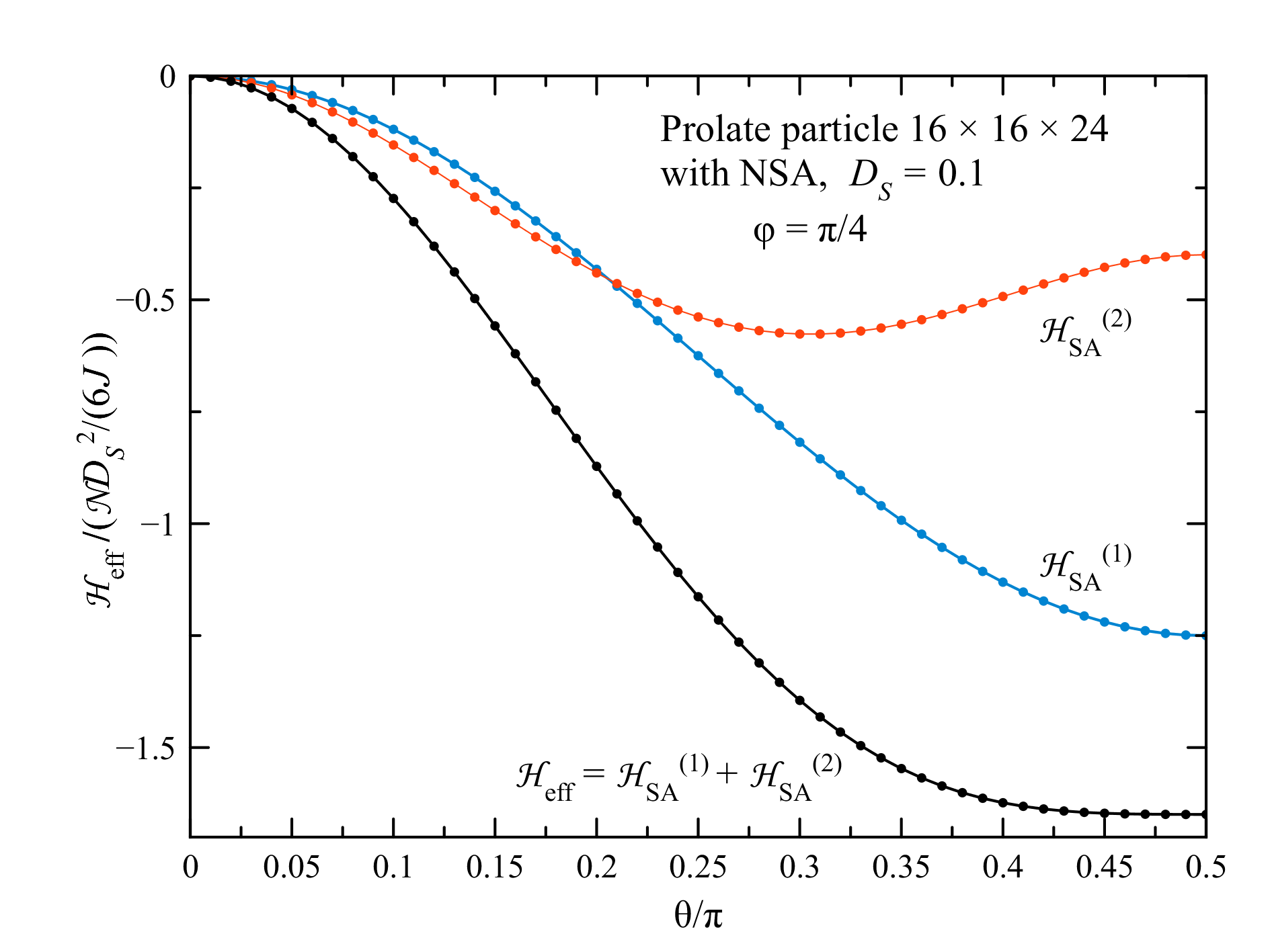
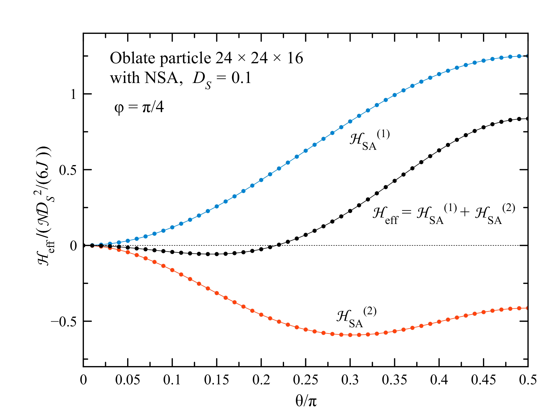
Figure 3: Energy landscape for prolate and oblate particles with SA. The second-order effective anisotropy computed as $\mathcal{H}_{SA}^{(2)}=\mathcal{H}_{\mathrm{eff}}-\mathcal{H}_{SA}^{(1)}$ is comparable with the first-order one. Upper panel: prolate particle. Lower panel: oblate particle.

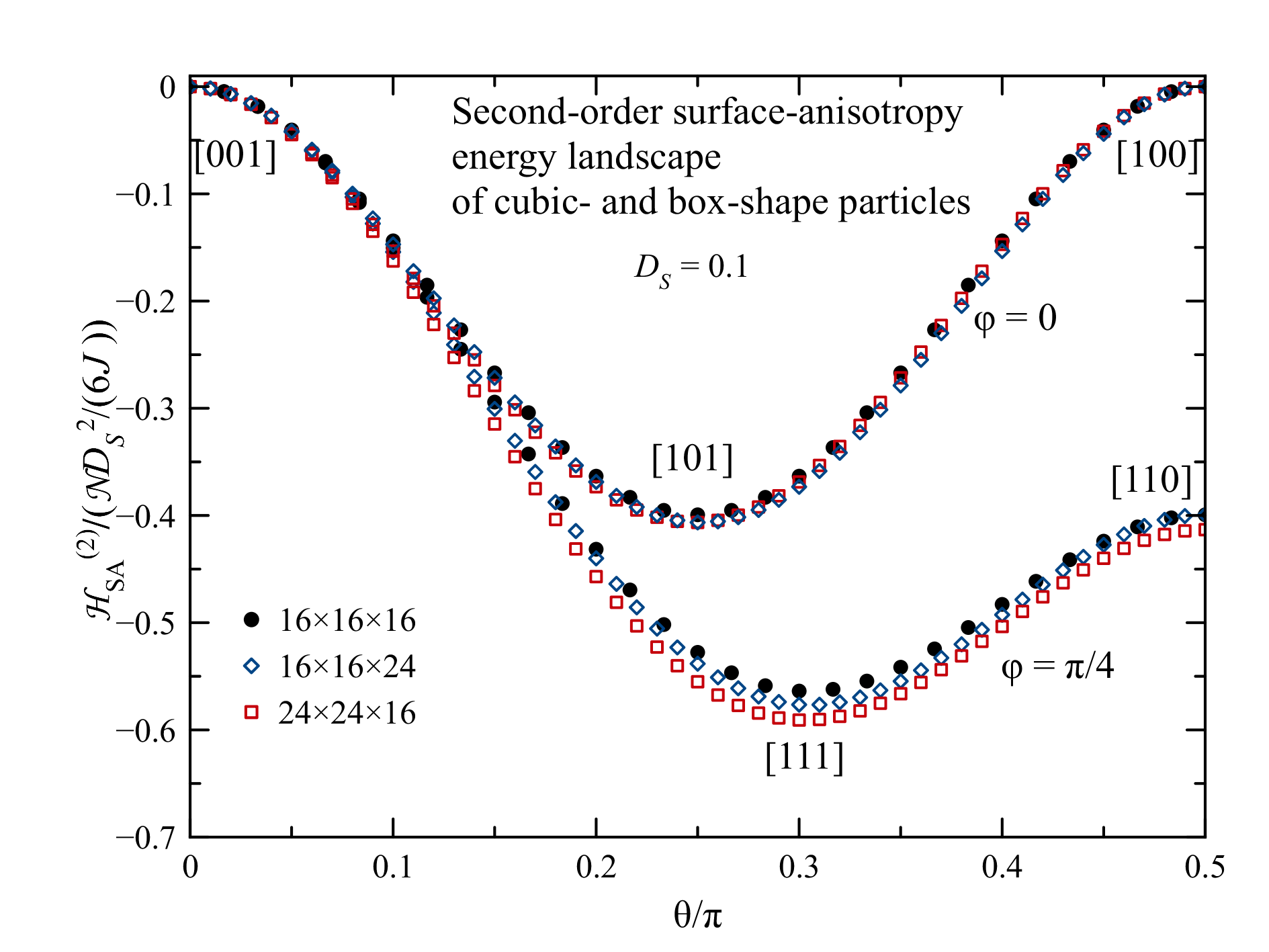
Figure 4: Second-order effective anisotropy for cubic, prolate, and oblate particles with SA. The result is practically independent of the particle’s aspect ratio.

The analytical solution for the second-order effective surface anisotropy is simpler for the cubic-shaped particle with the SA only. In this case, in the rigid-spin approximation, there is no effective field acting on the spin, so according to Eq. (16) there is no constrait field $\mathbf{h}_{\lambda}$ as well. (A similar problem was considered in Ref. Usov and Grebenshchikov (2008), however, no effective cubic anisotropy was obtained.) In the continuous approximation, the particle’s energy has the form

$$\mathcal{H}=\frac{1}{a^{3}}\intop dV\left[\frac{1}{2}a^{2}J\left(\frac{\partial s_{\alpha}}{\partial\mathbf{r}}\right)^{2}-\frac{1}{2}D_{S}a\delta_{S}\left(\mathbf{n}\cdot\mathbf{s}\right)^{2}\right]$$ (18)

with summation over the repeated $\alpha$. Here $\delta_{S}$ is the surface $\delta$-function and $\mathbf{n}$ is the outer normal to the surface. Minimizing this energy leads to the equation

$$\mathbf{s}\times\Delta\mathbf{s}=0$$ (19)

with the boundary condition

$$\mathbf{s}\times\left(a\frac{\partial\mathbf{s}}{\partial r_{\alpha}}n_{\alpha}-\frac{D_{S}}{J}\left(\mathbf{n}\cdot\mathbf{s}\right)\mathbf{n}\right)=0$$ (20)

at the surfaces.

Now, considering $D_{S}/J$ as small and starting from a collinear state of a fixed direction $\boldsymbol{\nu}$, one can consider surface-induced deviations $\boldsymbol{\boldsymbol{\psi}}$ from this state,

$$\mathbf{s}(\mathbf{r})=\boldsymbol{\nu}\sqrt{1-\boldsymbol{\boldsymbol{\psi}}^{2}(\mathbf{r})}+\boldsymbol{\boldsymbol{\psi}}(\mathbf{r})\cong\boldsymbol{\nu}\left[1-\frac{1}{2}\boldsymbol{\boldsymbol{\psi}}^{2}(\mathbf{r})\right]+\boldsymbol{\boldsymbol{\psi}}(\mathbf{r}),$$ (21)

where $\mathbf{s}(\mathbf{r})\cdot\boldsymbol{\boldsymbol{\psi}}(\mathbf{r})=0$ and $\boldsymbol{\boldsymbol{\psi}}$ satisfies the sum rule

$$\int d^{3}r\boldsymbol{\boldsymbol{\psi}}(\mathbf{r})=0.$$ (22)

Below $\boldsymbol{\psi}$ will be found within the linear approximation, whereas the quadratic term will be used to calculate the decrease of the particle’s magnetization $m$ – the magnetization deficit. The equation for $\boldsymbol{\boldsymbol{\psi}}$ becomes

$$\Delta\boldsymbol{\boldsymbol{\psi}}=0,\qquad a\frac{\partial\boldsymbol{\boldsymbol{\psi}}}{\partial r_{\alpha}}n_{\alpha}=\frac{D_{S}}{J}\mathbf{f}\left(\boldsymbol{\nu},\mathbf{n}\right),$$ (23)

where

$$\mathbf{f}\left(\boldsymbol{\nu},\mathbf{n}\right)\equiv\left(\mathbf{n}\cdot\boldsymbol{\nu}\right)\left[\mathbf{n}-\left(\mathbf{n}\cdot\mathbf{\boldsymbol{\nu}}\right)\mathbf{\boldsymbol{\nu}}\right]$$ (24)

is perpendicular to $\boldsymbol{\nu}$ and vanishes if $\mathbf{\boldsymbol{\nu}}$ is perpendicular to any particle’s face, $\mathbf{n}\cdot\mathbf{\boldsymbol{\nu}}=\pm 1$. For the parallelepiped of linear sizes $L_{x,y,z}$, the boundary conditions become

$$\pm a\left.\frac{\partial\boldsymbol{\boldsymbol{\psi}}}{\partial x}\right|_{x=\pm L_{x}/2}=\frac{D_{S}}{J}\mathbf{f}\left(\boldsymbol{\nu},\mathbf{n}\right)$$ (25)

etc. At the opposite faces of the particle $\mathbf{f}\left(\boldsymbol{\nu},\mathbf{n}\right)$ is the same as it is quadratic in $\mathbf{n}$. At different faces, $\mathbf{f}\left(\boldsymbol{\nu},\mathbf{n}\right)$ are, in general, different. The explicit values are given by

$$\mathbf{f}\left(\boldsymbol{\nu},\mathbf{n}\right)=\begin{cases}\nu_{x}\left(\mathbf{e}_{x}-\nu_{x}\boldsymbol{\nu}\right),&x=\pm L_{x}/2\\ \nu_{y}\left(\mathbf{e}_{y}-\nu_{y}\boldsymbol{\nu}\right),&y=\pm L_{y}/2\\ \nu_{z}\left(\mathbf{e}_{z}-\nu_{z}\boldsymbol{\nu}\right),&z=\pm L_{z}/2.\end{cases}$$ (26)

For the cube of linear size $L$, one can search for the solution in the form

$$\boldsymbol{\psi}(\mathbf{r})=\frac{D_{S}}{LaJ}\left(\mathbf{C}_{x}x^{2}+\mathbf{C}_{y}y^{2}+\mathbf{C}_{z}z^{2}\right)$$ (27)

that satisfies the Laplace equation and at the same time Eq. (22) for

$$\mathbf{C}_{x}+\mathbf{C}_{y}+\mathbf{C}_{z}=0.$$ (28)

From the boundary conditions above one finds

$$\mathbf{C}_{x,y,z}=\left.\mathbf{f}\left(\boldsymbol{\nu},\mathbf{n}\right)\right|_{x,y,z=\pm L/2},$$ (29)

the values from Eq. (26). One can check that this solution satisfies Eq. (28).

The maximal value of $\psi$ reached at the surfaces of the particle should be small,

$$\psi\sim\frac{L}{a}\frac{D_{S}}{J}\ll 1,$$ (30)

that defines the applicability range of the linearization. For $\nu_{x}=\nu_{y}=\nu_{z}=1/\sqrt{3}$ at the center of the face $x=L/2$, $y=z=0$ one has $6\sqrt{2}\simeq 8.5$ in the denominator of this formula, thus the applicability condition is milder than above. On the other hand, there are instabilities of the found states at larger $L$ and $D_{S}$ that were observed numerically but haven’t been yet worked out analytically. These instabilities also limit the applicability of the method.

Now the particle’s magnetization can be computed using the quadratic terms in Eq. (21) as

$$\mathbf{m}=\frac{1}{V}\iiintop_{0}^{L}dxdydz\left\{\boldsymbol{\nu}\left[1-\frac{1}{2}\boldsymbol{\boldsymbol{\psi}}^{2}(\mathbf{r})\right]+\boldsymbol{\boldsymbol{\psi}}(\mathbf{r})\right\}.$$ (31)

Here the linear term vanishes while the quadratic term yields

$$\mathbf{m}=\boldsymbol{\nu}\left[1-\frac{1}{360}\left(\frac{L}{a}\frac{D_{S}}{J}\right)^{2}\left(1-\nu_{x}^{4}-\nu_{y}^{4}-\nu_{z}^{4}\right)\right].$$ (32)

Clearly, the magnetization deficit vanishes if $\mathbf{\boldsymbol{\nu}}$ is perpendicular to any particle’s face and reaches its maximum for the grand-diagonal directions $\left(\pm 1,\pm 1,\pm 1\right)$. Again, the small coefficient in this formula suggests that the applicability condition for the linearization method is milder than given by Eq. (30).

The energy of the particle for the state found above at the lowest, quadratic, order in $D_{S}$ becomes

$$\mathcal{H}_{SA}^{(2)}=\intop\frac{dV}{a^{3}}\left[\frac{1}{2}a^{2}J\left(\frac{\partial\psi_{\alpha}}{\partial\mathbf{r}}\right)^{2}-D_{S}a\delta_{S}\left(\mathbf{n}\cdot\boldsymbol{\nu}\right)\left(\mathbf{n}\cdot\boldsymbol{\psi}\right)\right],$$ (33)

i.e., $\mathcal{H}_{SA}^{(2)}=E_{ex}+E_{DS}$. After integration one obtains

$$\mathcal{H}_{SA}^{(2)}=-\frac{\mathcal{N}D_{S}^{2}}{6J}\left(1-\nu_{x}^{4}-\nu_{y}^{4}-v_{z}^{4}\right),$$ (34)

whereas $E_{ex}=-\mathcal{H}_{SA}^{(2)}>0$ and $E_{DS}=2\mathcal{H}_{SA}^{(2)}<0$. This result is similar to that for the spherical particle Garanin and Kachkachi (2003) and differs from it by the missing factor $\kappa\simeq 0.53.$ Adding the first-order effective particle’s Hamiltonian, Eq. (3), one obtains

$$\mathcal{H}_{\mathrm{eff}}=-\mathcal{N}_{\mathrm{core}}Ds_{z}^{2}-\mathcal{N}\mathbf{h}\cdot\mathbf{s}+\mathcal{H}_{SA}^{(1)}+\mathcal{H}_{SA}^{(2)},$$ (35)

where $\mathcal{H}_{SA}^{(1,2)}$ are given by Eqs. (4) and (34), respectively. This additive approximation does not take into account screening and is good for not too large particle’s sizes $L$.

VI Numerical results

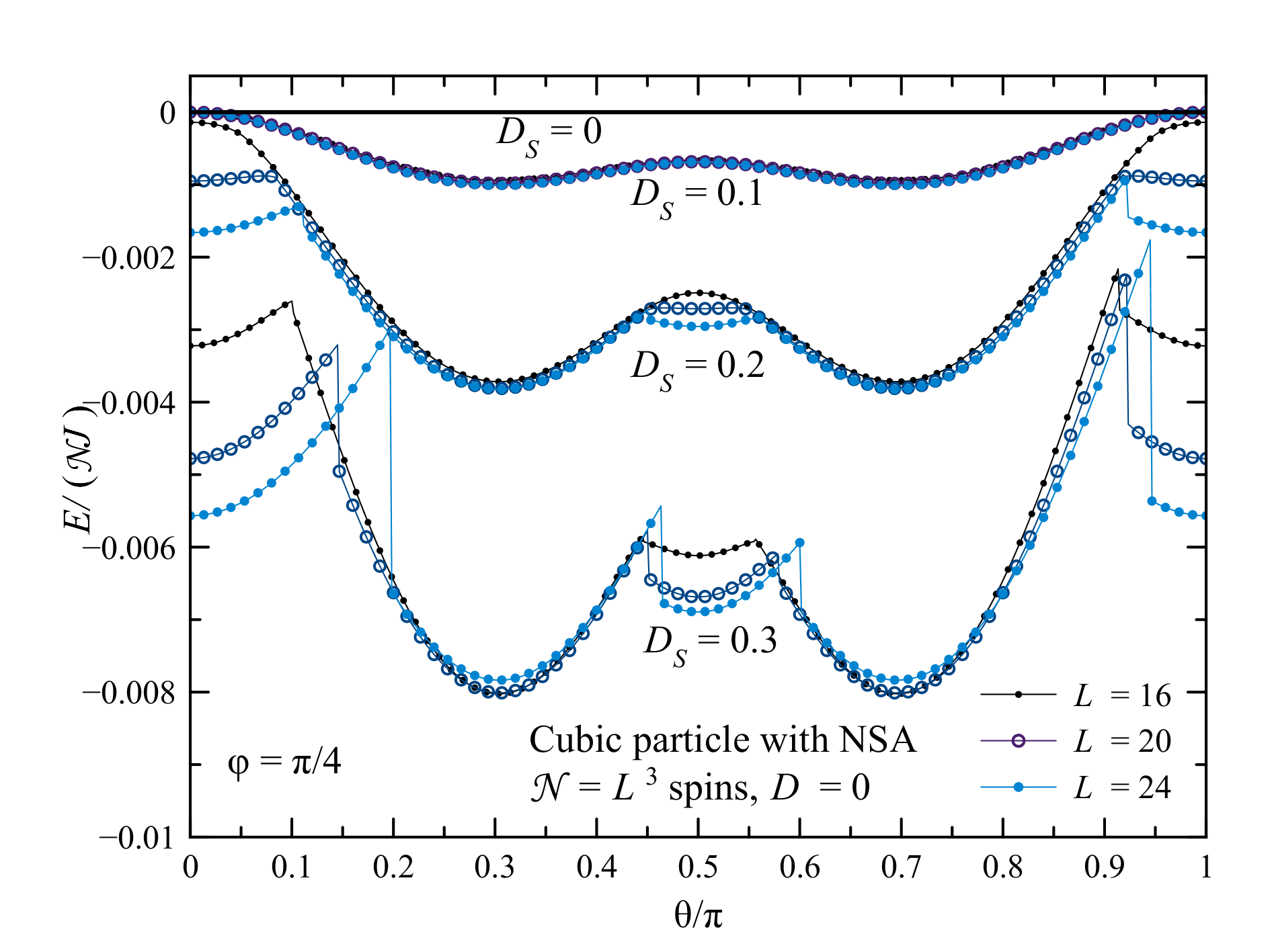
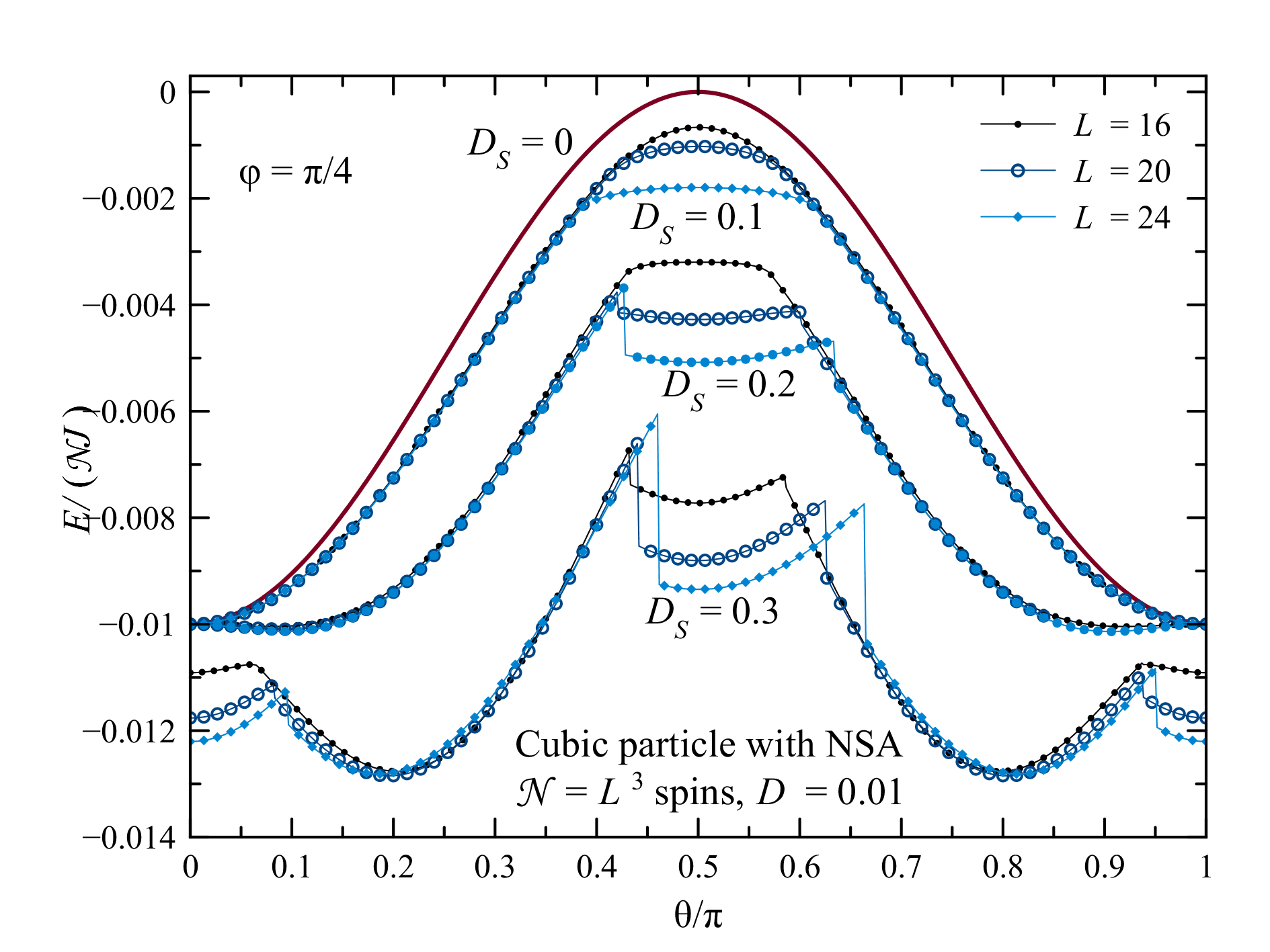
Figure 5: Energy landscapes for cubic particles with the surface and core anisotropies: Numerical results for the particle sizes $L=16$, 20, 24 and the SA strenghts $D_{S}=0.1,$ 0.2, 0.3. For larger $L$ and $D_{S}$, the barrier in the middle is lowered because of the instability leading to deviations from the single-domain state. For even larger $L$ and $D_{S}$, the result of the constrained energy minimization becomes multi-valued. Upper panel: $D=0$. Lower panel: $D=0.01$.

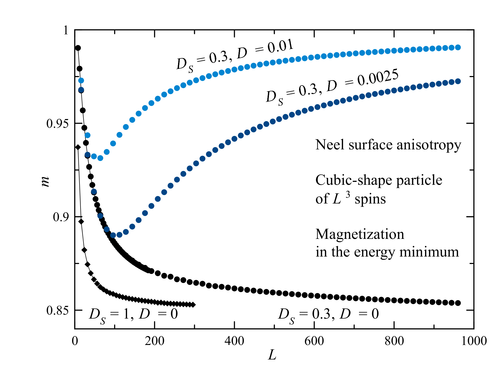
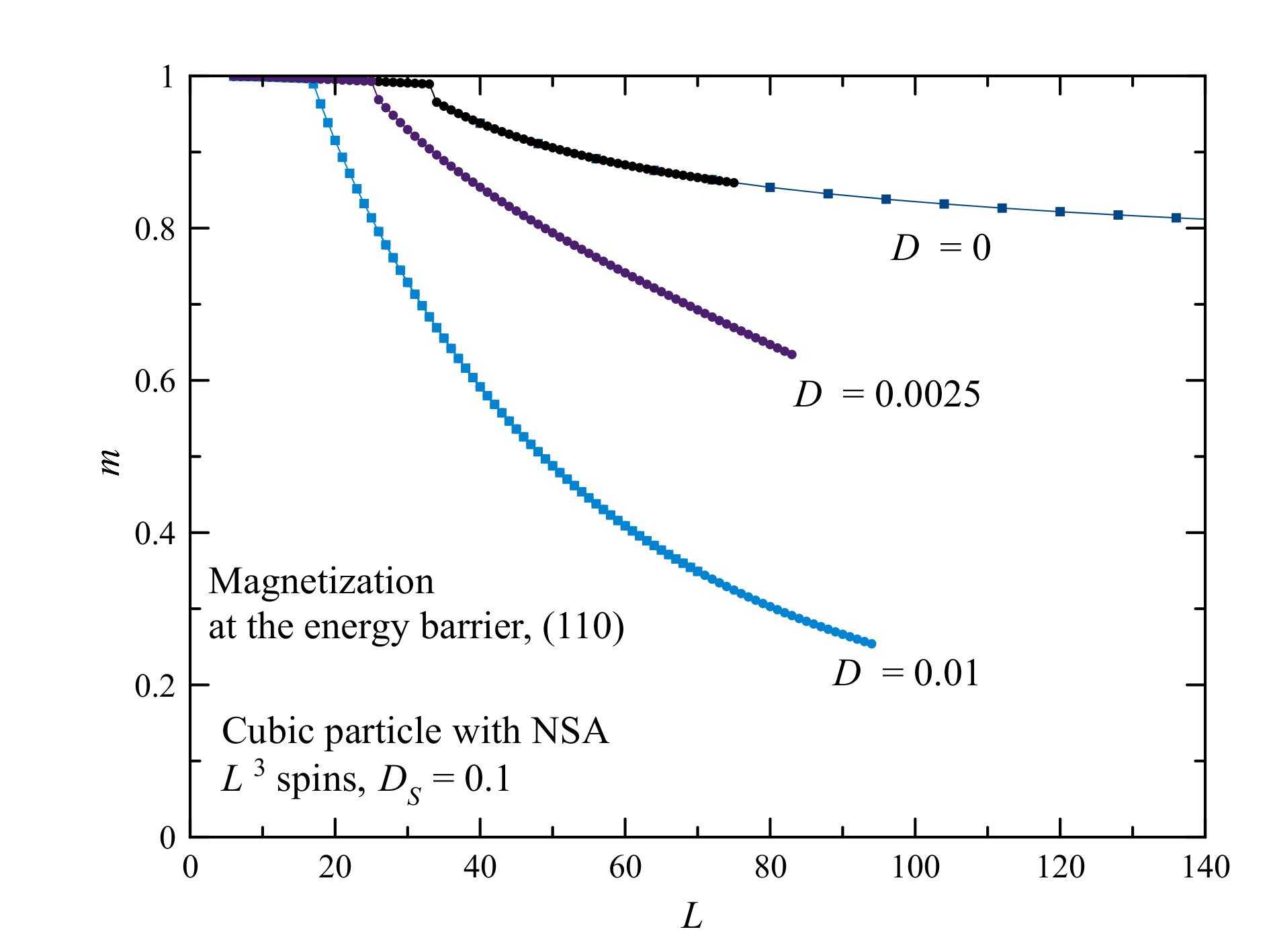
Figure 6: Particle’s magnetization $m$ vs its linear size $L$ for $D_{S}=0.1$ and different values of the core anisotropy $D$. Upper panel: magnetization in the direction of the energy minimum, $\left(1,1,1\right)$ for $D=0$. Here $D>0$ stabilizes the quasi-collinear state by screening the surface perturbations. Lower panel: magnetization in the direction of the energy barrier, $\left(1,1,0\right)$. Here $D>0$ destabilizes the quasi-collinear state because of the tendency to form a domain wall across the particle.

Fig. 1 shows the energy landscapes of cubic particles of sizes $L=16$ and 32 computed by the constrained energy minimization as explained in Sec. IV together with the analytical result of Eq. (34). There is a fair overall agreement between the numerical and analytical results, although Eq. (34) shows deeper energy minima. The discrepansy must be due to finite-size effects. Indeed, each face contains only $(L-2)^{2}$ sites subject to the SA rather than $L^{2}$ sites. This suggests renormalization of $D_{S}$ as $D_{S}\Rightarrow\tilde{D}_{S}=(1-2/L)^{2}D_{S}$ that results in the additional factor $(1-2/L)^{4}$ in $\mathcal{H}_{SA}^{(2)}$. However, this renormalization would be too strong for the results in Fig. 1 making the energy minima a way too shallow. However, there are edges working in the same directions as faces, only weaker. Also the exchange interaction weakens near the surfaces because of the missing neighbors. In the absence of an analytical solution for the lattice problem, one can fit the finite-size effect replacing the effective number of spins in the face by $(L-\varsigma)^{2}$. The results of Eq. (34) with the additional factor $(1-\varsigma/L)^{4}$ with $\varsigma=0.7$ in $\mathcal{H}_{SA}^{(2)}$ shown in Fig. 1 as “Analytical, finite size” are closer to the numerical results than the pure results of Eq. (34) labeled “Analytical”.

Whereas for $L=16$ the numerical results for the two different values of $D_{S}$ scale, for $L=32$ there are visible deviations from scaling. In particular, for $D_{S}=0.1$ the energy of the $\left(0,0,1\right)$ state is lowered due to the instability of the collinear state in which spins near some surfaces turn by $90^{\circ}$under the influence of the SA. This can be seen in the lower panel of Fig. 2. This state cannot be obtained within the linear approximation. For $L=16$ there is still no instability and the $\left(0,0,1\right)$ state is strictly collinear. On the other hand, the $\left(1,1,0\right)$ state in the upper panel of Fig. 2 is that given by Eq. (27) and its numerically found magnetization is $m=0.9898$ while Eq. (32) yields a close value $m=0.9858$. On the other hand, the magnetization in the unstable $\left(0,0,1\right)$ state for $L=32$ is lower: $m=0.9680$.

Numerical results for the energy landscape of prolate and oblate box-shape particles with $D_{S}=0.1$ are shown in Fig. 3. In this case there is the first-order contribution to the effective anisotropy $\mathcal{H}_{SA}^{(1)}$ given by Eq. (5). The second-order term can be computed as the difference: $\mathcal{H}_{SA}^{(2)}=\mathcal{H}_{\mathrm{eff}}-\mathcal{H}_{SA}^{(1)}$, where $\mathcal{H}_{\mathrm{eff}}$ is the numerically obtained particle’s energy. One can see that the second-order term can be large enough to compete with the first-order one. For prolate and oblate particles, $\mathcal{H}_{SA}^{(2)}$ is very close to the cubic-particle result, as shown in Fig. 4.

Fig. 5 shows the energy landscapes for three different particle’s sizes and three different values of $D_{S}$ for the core anisotropy $D=0$ and $D=0.01$. In contrast to Fig. 1, the energy is shown not scaled with $D_{S}^{2}$. One can see that for larger $L$ and $D_{S}$ the barrier in the middle is flattened and lowered because of the instability leading to the deviation from the single-domain barrier state with all spins perpendicular to $z$ axis. As the result of this instability, spins on one side of the cube turn toward $z$ axis to lower the energy, whereas spins on the other side turn in the opposite direction Garanin (3988). Further increasing $L$ results in forming a domain wall in the middle of the particle, and the constrained energy minimization fails. This state cannot be obtained within the linear approximation. The lower panel of 5 shows the energy landscape dominated by the core anisotropy, however, strongly modified by the SA. Here, too, the uniform barrier state is destroyed for large particles and strong SA.

Dependence of the particle’s magnetization on the particle’s size $L$ is shown in Fig. 6. The role of the core anisotropy $D$ is strikingly different for the energy-mimina and the energy-barrier states. For $D=0$ at the minima at $\left(\pm 1,\pm 1,\pm 1\right)$, the magnetization deficit is growing with $L$ according to Eq. (32), so $m$ goes down. However, for larger $L$ the saturation state is reached in which the surface spins are oriented according to the SA (perpendicular to the surfaces near the surfaces for $D_{S}>0$). In this state, instead of Eq. (27), $\boldsymbol{\psi}(\mathbf{r})$ [or, rather, $\mathbf{s}(\mathbf{r})$] is a function of $\mathbf{r}/L$ only, independently of $a$. Thus $m$ becomes a geometrical constant $m\simeq 0.85$ independent of $L$ and $D_{S}$. For $D>0$, perturbations from the surface become screened at the distance of the domain-wall width $\delta=\sqrt{J/(2D)}$. Thus on increasing $L$ the magnetization $m$ at first decreases until $L\sim\delta$, then increases again because of the screening. This is clearly seen in the upper panel of Fig. 6 where the extremely large values of $L$ should be noticed.

In the lower panel of Fig. 6, the magnetization in the barrier state $\left(110\right)$ is close to 1 for $L$ small enough, while the spin configuration is shown in the upper panel of Fig. 2. Further increase of $L$ causes instabilities of the surface spins in the $xy$ surfaces: for $D_{S}>0$ these spins turn perpendicular to the surfaces parallel $z$ axis. In the limit $L\rightarrow\infty$ for $D=0$, a state with $\mathbf{s}(\mathbf{r})$ depending on $\mathbf{r}/L$ only should be reached, in which $m$ is a another geometrical constant. However, $D>0$ leads to the instability at smaller $L$ with the subsequent formation of a domain wall in the middle of the particle. After that the constrained energy minimization method fails, that’s why the $D>0$ curves in the lower panel of Fig. 6 could not be computed for larger $L$. To the contrary, $D_{S}<0$ stabilizes surface spins in the $xy$ planes, so that the discussed instability does not happen for $D=0$ and requires the values of $D$ exceeding some threshold to develop.

VII Screening and other generalizations

In this section the results of Sec. V will be generalized for the model with the uniaxial anisotropy and magnetc field. Some calculations will be made for a parallelepiped particle where the first-order effective surface anisotropy is present. In the continuous approximation, the Hamiltonian has the form

$$\mathcal{H}=\intop\frac{dV}{a^{3}}\left[\frac{a^{2}J}{2}\left(\frac{\partial s_{\alpha}}{\partial\mathbf{r}}\right)^{2}-Ds_{z}^{2}-\mathbf{h}\cdot\mathbf{s}-\frac{D_{S}}{2}a\delta_{S}\left(\mathbf{n}\cdot\mathbf{s}\right)^{2}\right].$$ (36)

Using Eq. (21), from the first of equations (9) one obtains

$$0=(\boldsymbol{\nu}+\boldsymbol{\psi})\times\left[\mathbf{h}+2D\left(\nu_{z}+\psi_{z}\right)\mathbf{e}_{z}+a^{2}J\Delta\boldsymbol{\psi}+\mathbf{h}_{\lambda}\right],$$ (37)

where $\mathbf{h}_{\lambda}$ is given by Eq. (16). The boundary conditions are defined by Eq. (25). Substituting $\mathbf{h}_{\lambda}$ and rearranging keeping only the linear-$\boldsymbol{\psi}$ terms, one arrives at

$$\boldsymbol{\nu}\times\left[2D\psi_{z}\mathbf{e}_{z}+a^{2}J\Delta\boldsymbol{\psi}-\mathbf{h}_{SA}\right.$$

$$-\left.\boldsymbol{\nu}\cdot\left(\mathbf{h}+2D\nu_{z}\mathbf{e}_{z}+\mathbf{h}_{SA}\right)\boldsymbol{\psi}\right] = 0.$$ (38)

One can search for the solution in the form

$$\boldsymbol{\psi}=\psi_{1}\boldsymbol{\nu}_{1}+\psi_{2}\mathbf{\boldsymbol{\nu}}_{2},$$ (39)

where $\mathbf{\boldsymbol{\nu}}_{1}$ and $\mathbf{\boldsymbol{\nu}}_{2}$ are unit vectors perpendicular to $\boldsymbol{\nu}$ and to each other, so that $\boldsymbol{\nu}\times\mathbf{\boldsymbol{\nu}}_{1}=\mathbf{\boldsymbol{\nu}}_{2}$. It is convenient to choose $\mathbf{\boldsymbol{\nu}}_{1}\cdot\mathbf{e}_{z}=0$ and $\mathbf{\boldsymbol{\nu}}_{2}$ in the plane spanned by $\mathbf{e}_{z}$ and $\boldsymbol{\nu}$. Then equations for $\psi_{1}$ and $\psi_{2}$ decouple, and after some algebra one obtains Helmholtz equations with sources

$$\Delta\psi_{1}-\kappa_{1}^{2}\psi_{1} = \mathbf{\boldsymbol{\nu}}_{1}\cdot\mathbf{h}_{SA}$$

$$\Delta\psi_{2}-\kappa_{2}^{2}\psi_{2} = \mathbf{\boldsymbol{\nu}}_{2}\cdot\mathbf{h}_{SA},$$ (40)

where

$$\kappa_{1}^{2} \equiv \frac{\mathbf{\boldsymbol{\nu}}\cdot\left(\mathbf{h}+\mathbf{h}_{SA}\right)+2D\nu_{z}^{2}}{a^{2}J}$$

$$\kappa_{2}^{2} \equiv \frac{\mathbf{\boldsymbol{\nu}}\cdot\left(\mathbf{h}+\mathbf{h}_{SA}\right)+2D\left(2\nu_{z}^{2}-1\right)}{a^{2}J}.$$ (41)

Here $\kappa^{2}>0$ corresponds to the exponentially decaying perturbations (screening), whereas $\kappa^{2}<0$ describes proliferating perturbations (anti-screening). For instance, for $h=h_{SA}=0$ and $\nu_{z}>1/\sqrt{2}$ $\left(\theta<\pi/4\right)$ both $\kappa_{1}^{2}$ and $\kappa_{2}^{2}$ are positive and the uniaxial anisotropy stabilizes the particle’s magnetization. Larger deviations from the easy axis lead to $\kappa_{2}^{2}<0$ and destruction of the particle’s magnetization. For the source terms in the case $N_{x}=N_{y}\equiv N_{\bot}$ from Eq. (15) one obtains

$$\mathbf{\boldsymbol{\nu}}_{1}\cdot\mathbf{h}_{SA}=0,\qquad\mathbf{\boldsymbol{\nu}}_{2}\cdot\mathbf{h}_{SA}=-2D_{S}\frac{N_{\bot}-N_{z}}{N_{\bot}N_{z}}\nu_{z}\sqrt{1-\nu_{z}^{2}}.$$ (42)

In the sequel, we consider cubic particles for which $\mathbf{h}_{SA}=0$. The solution of Eqs. (40) can be searched for in the form

$$\psi_{\alpha}=\frac{D_{S}}{aJ}\frac{C_{\alpha x}\cosh\kappa_{\alpha}x+C_{\alpha y}\cosh\kappa_{\alpha}y+C_{\alpha z}\cosh\kappa_{\alpha}z}{\kappa_{\alpha}\sinh\left(\kappa_{\alpha}L/2\right)},$$ (43)

where $\alpha=1,2$ and $\boldsymbol{\psi}$ is defined by Eq. (39). This function satisfies the Helmholtz equations, if the sum of the $C$-coefficients is zero. They can be determined from the boundary conditions, Eq. (25). Using Eq. (26), one obtains

$$C_{\alpha x} = \left.f_{\alpha}\left(\boldsymbol{\nu},\mathbf{n}\right)\right|_{x=L/2}=\nu_{x}\nu_{\alpha x}$$

$$C_{\alpha y} = \left.f_{\alpha}\left(\boldsymbol{\nu},\mathbf{n}\right)\right|_{y=L/2}=\nu_{y}\nu_{\alpha y}$$

$$C_{\alpha z} = \left.f_{\alpha}\left(\boldsymbol{\nu},\mathbf{n}\right)\right|_{z=L/2}=\nu_{z}\nu_{\alpha z},$$ (44)

where $\nu_{\alpha x}=\boldsymbol{\nu}_{\alpha}\cdot\mathbf{e}_{x}$, etc. One can see that

$$C_{\alpha x}+C_{\alpha y}+C_{\alpha z}=\boldsymbol{\nu}\cdot\boldsymbol{\nu}_{\alpha}=0,$$ (45)

as it should be. With the current choice of the vectors $\mathbf{\boldsymbol{\nu}}_{1}$ and $\mathbf{\boldsymbol{\nu}}_{2}$, the explicit form of the $C$-coefficients is

$$C_{1x}=-C_{1y}=\frac{\nu_{x}\nu_{y}}{\sqrt{1-\nu_{z}^{2}}},\qquad C_{1z}=0,$$ (46)

and

$$C_{2x}=C_{2y}=\frac{\nu_{y}^{2}\nu_{z}}{\sqrt{1-\nu_{z}^{2}}},\qquad C_{2z}=-\nu_{z}\sqrt{1-\nu_{z}^{2}}.$$ (47)

In the case $\kappa=ik$ (the anti-screening case), Eq. (43) becomes

$$\psi_{\alpha}=-\frac{D_{S}}{aJ}\frac{C_{\alpha x}\cos k_{\alpha}x+C_{\alpha y}\cos k_{\alpha}y+C_{\alpha z}\cos k_{\alpha}z}{k_{\alpha}\sin\left(k_{\alpha}L/2\right)}.$$ (48)

At $k_{\alpha}\rightarrow 0$ this expression is regular but it diverges at $k_{\alpha}L\rightarrow 2\pi$. For instance, for $h=0$ and $\nu_{z}=0$ in Eq. (41) one has $k_{2}=1/\delta,$ so that the particle’s size should satisfy $L<2\pi\delta$. However, in the model with a uniaxial ansotropy there is another stability criterion Garanin (3988), $L<\pi\delta$, for the same state with the spin perpendicular to the easy axis – the barrier state. If this condition is violated, then there is a finite $\psi$ even in the absence of the surface anisotropy. Thus, the divergence of the solution at $L=2\pi\delta$ is beyond the applicability range of the linearization method. For $D=0$, there is no corresponding instability, but screening and antiscreening can be created by the magnetic field. In this case, the point $k_{\alpha}L=2\pi$ can be approached, and this defines the applicability of the method.

The energy of the particle at second order in $\boldsymbol{\psi}$ is given by Eq. (33) with the additional term $-D\psi_{z}^{2}$ in square brackets. The terms linear in $\boldsymbol{\psi}$ vanish because of Eq. (22). After some algebra one arrives at the final result

$$\mathcal{H}_{\mathrm{eff}} = -\mathcal{N}\left(D\nu_{z}^{2}+\mathbf{h}\cdot\boldsymbol{\nu}\right)-\frac{\mathcal{N}D_{S}^{2}}{3J}\left[\frac{\nu_{x}^{2}\nu_{y}^{2}}{1-\nu_{z}^{2}}F\left(\kappa_{1}L\right)\right.$$ (49)

$$+\left.\left(\nu_{z}^{2}\left(\nu_{x}^{2}+\nu_{y}^{2}\right)-\frac{\nu_{x}^{2}\nu_{y}^{2}\nu_{z}^{2}}{1-\nu_{z}^{2}}\right)F\left(\kappa_{2}L\right)\right]$$

$$-\frac{L^{2}}{\delta^{2}}\frac{\mathcal{N}D_{S}^{2}}{J}\nu_{z}^{2}\left(\nu_{x}^{4}+\nu_{y}^{4}+\nu_{x}^{2}\nu_{y}^{2}\right)F_{D}\left(\kappa_{2}L\right),$$

where $\delta=a\sqrt{J/(2D)}$,

$$F(x)=\frac{3}{x}\frac{3\sinh\left(x\right)+x}{\cosh\left(x\right)-1}-\frac{24}{x^{2}}\cong\begin{cases}1-\frac{x^{4}}{2520},&x\ll 1\\ \frac{9}{x}-\frac{24}{x^{2}},&x\gg 1\end{cases}$$ (50)

and

$$F_{D}(x)=\frac{1}{x^{3}}\frac{\sinh\left(x\right)+x}{\cosh\left(x\right)-1}-\frac{4}{x^{4}}\cong\begin{cases}\frac{1}{180}-\frac{x^{2}}{3780},&x\ll 1\\ \frac{1}{x^{3}}-\frac{4}{x^{4}},&x\gg 1.\end{cases}.$$ (51)

In the case of $\kappa=ik$ one has to replace $F\left(ikL\right)\Rightarrow G(kL),$ where

$$G(x)=\frac{24}{x^{2}}-\frac{3}{x}\frac{3\sin\left(x\right)+x}{1-\cos\left(x\right)}$$ (52)

has the same behavior as $F(x)$ at $x\ll 1$ but diverges at $x=2\pi$. The last term in Eq. (49) is the cross-term originating from $-D\psi_{z}^{2}$ in the integrand of the energy.

For $D=0$, one has $\kappa_{1}=\kappa_{2}=\kappa$, and the energy simplifies to

$$\mathcal{H}_{\mathrm{eff}} = -\mathcal{N}\mathbf{h}\cdot\boldsymbol{\nu}-\frac{\mathcal{N}D_{S}^{2}}{3J}F\left(\frac{L}{a}\sqrt{\frac{\mathbf{h}\cdot\boldsymbol{\nu}}{J}}\right)$$ (53)

$$\qquad\times\left(\nu_{x}^{2}\nu_{y}^{2}+\nu_{y}^{2}\nu_{z}^{2}+\nu_{z}^{2}\nu_{x}^{2}\right).$$

Here there can be screening or anti-screening because of the magnetic field. For $h=0$, Eq. (34) is recovered.

In the limit of $\kappa_{1}L,\kappa_{2}L\ll 1$, the second-order part of Eq. (49) simplifies to Eq. (34). In this case, the first- and second-order terms in the effective particle’s anisotropy are additive. The leading correction term of order $\left(L/\delta\right)^{2}$ comes from the cross-term in the energy with a small numerical factor. The corrections from the terms with the function $F$ are of order $\left(L/\delta\right)^{4}$ with an extremely small numerical factor.

Energy landscapes plotted using Eq. (49) for $L$ small enough show very small deviations from the results obtained using the additive effective Hamiltonian, Eq. (35). For larger $L$, some deviations are seen but then, with the further inclease of $L$, the solution quickly diverges for the orientations having the imaginary $\kappa$ – near the barriers and opposite to the magnetic field, where anti-screening occurs. As an example, hysteresis loops for $\mathbf{H}$ along $z$ axis are shown in Fig. 7. The results of the additive model do not depend on $L/\delta$. The exact results using Eq. (49) are very close to the latter for $L/\delta\lesssim 5$. However, for $L/\delta\gtrsim 5$ the solution diverges and the hysteresis loop breaks down.

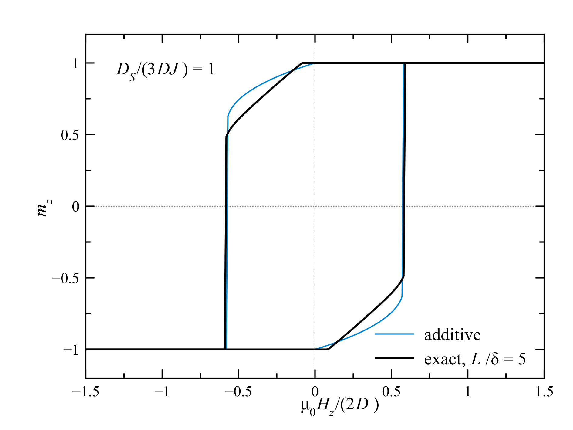
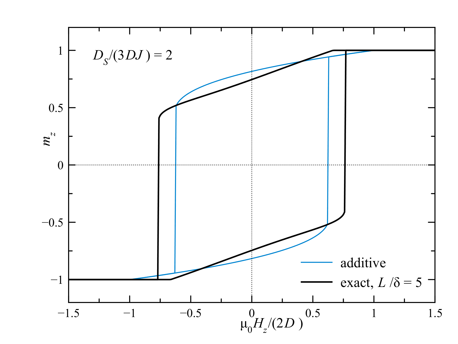
Figure 7: Hysteresis loops for $\mathbf{H}$ along $z$ axis, using the additive effective particle’s Hamiltonian, Eq. (35), and the exact analytical solution, Eq. (49), that depends on the ratio $L/\delta$.

For the field along $z$ axis, the energy of the particle can be minimized with respect to the azimuthal angle $\varphi$ that yields $\varphi=\pi/4$ and equivalent solutions. For these values of $\varphi$, one can write down the compact expression of the energy in terms of $x\equiv\cos\theta$. Eq. (49) in the reduced form becomes

$$e(x) = -x^{2}-2\alpha x-\frac{1}{4}\beta\left(1-x^{2}\right)\left[F\left(\kappa_{1}L\right)+3x^{2}F\left(\kappa_{2}L\right)\right]$$ (54)

$$\qquad-\frac{9}{4}\beta x^{2}\left(1-x^{2}\right)^{2}\tilde{L}^{2}F_{D}\left(\kappa_{2}L\right),$$

where

$$e\equiv\frac{\mathcal{H}_{\mathrm{eff}}}{\mathcal{N}D},\quad\alpha\equiv\frac{h}{2D},\quad\beta\equiv\frac{D_{S}^{2}}{3DJ},\quad\tilde{L}\equiv\frac{L}{\delta}$$ (55)

and

$$\kappa_{1}L=\tilde{L}\sqrt{\alpha x+x^{2}},\qquad\kappa_{2}L=\tilde{L}\sqrt{\alpha x+2x^{2}-1}.$$ (56)

In the case of zero field and dominating uniaxial anisotropy, the dimensionless energy barrier is given by

$$u=e(0)-e(1)=1-\frac{1}{4}\beta.$$ (57)

It does not depend on screening and is the same as within the additive approximation. To investigate the stability of the state along $z$ axis, $x=1$, one can expand $e(x)$ in terms of $\delta x\equiv 1-x$. This yields

$$e\cong-1-2\alpha+2\left[1+\alpha-\beta F\left(\tilde{L}\sqrt{1+\alpha}\right)\right]\delta x$$ (58)

thus the energy minimum is stable for

$$\frac{1+\alpha}{F\left(\tilde{L}\sqrt{1+\alpha}\right)}>\beta.$$ (59)

For small particles screening is negligible, $F\cong 1$, and one obtains the condition $1+\alpha>\beta$. For large particles, one uses the asymptotic form $F(x)\cong 9/x$ that results in the condition $\left(1+\alpha\right)^{3/2}>9\beta/\tilde{L}$ that means a greater stability against the surface effects parametrized by $\beta$. In the upper panel of Fig. 7, $\beta=1$, so that within the additive approximation the energy minimum $x=1$, i.e., $m_{z}=1$ exists for $\alpha>0$, i.e., $H>0$. Screening in the exact solution makes this energy minimum more stable, so that it disappears at the negative field corresponding to $\alpha=\left(9\beta/\tilde{L}\right)^{2/3}-1$, as can be seen in Fig. 7. These results are also related to precession frequencies near energy minima and can be important for the magnetic resonance in magnetic nanoparticles Kachkachi and Schmool (2007); Bastardis et al. (2017).

VIII Thermally-activated magnetization switching

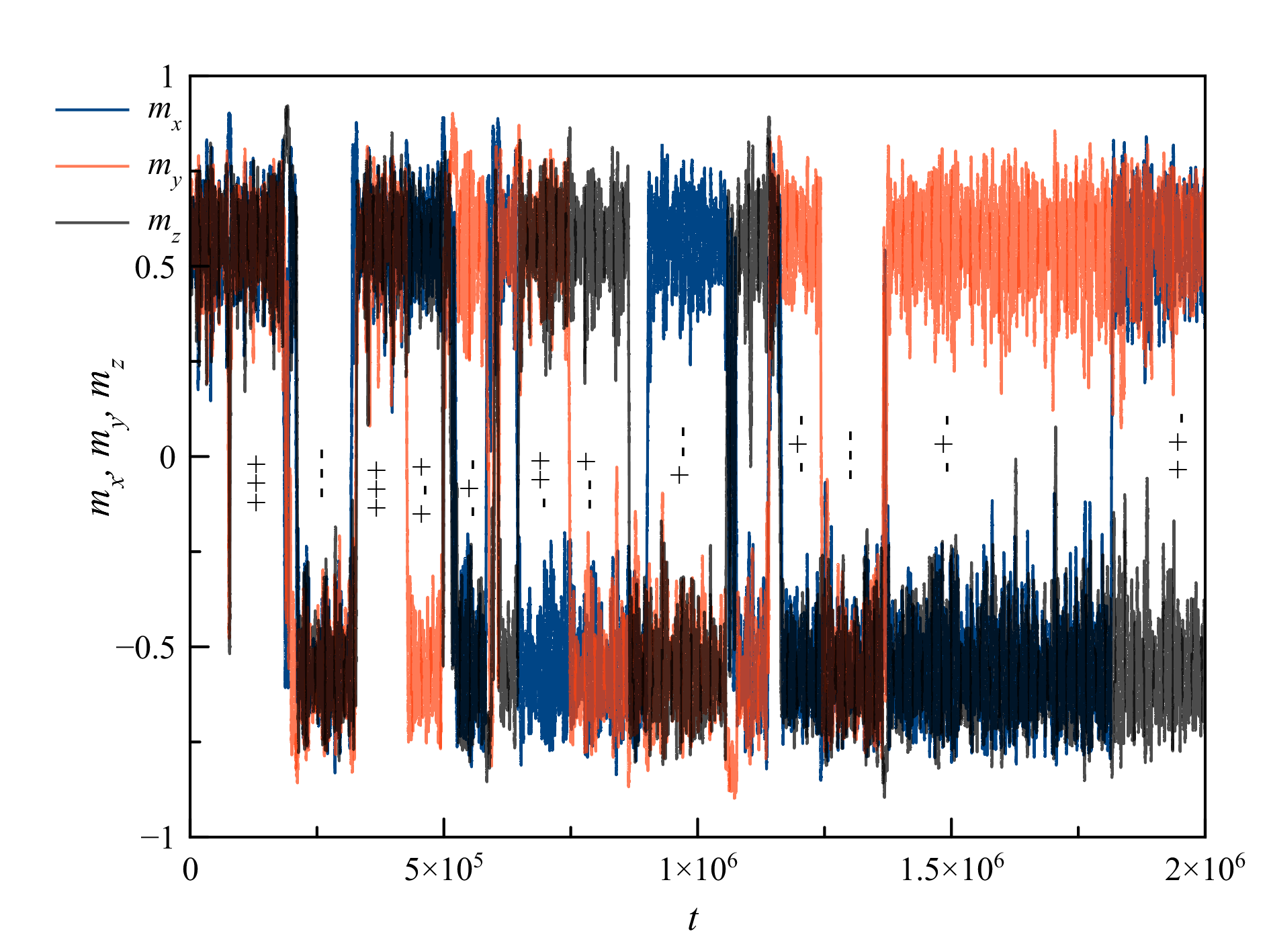
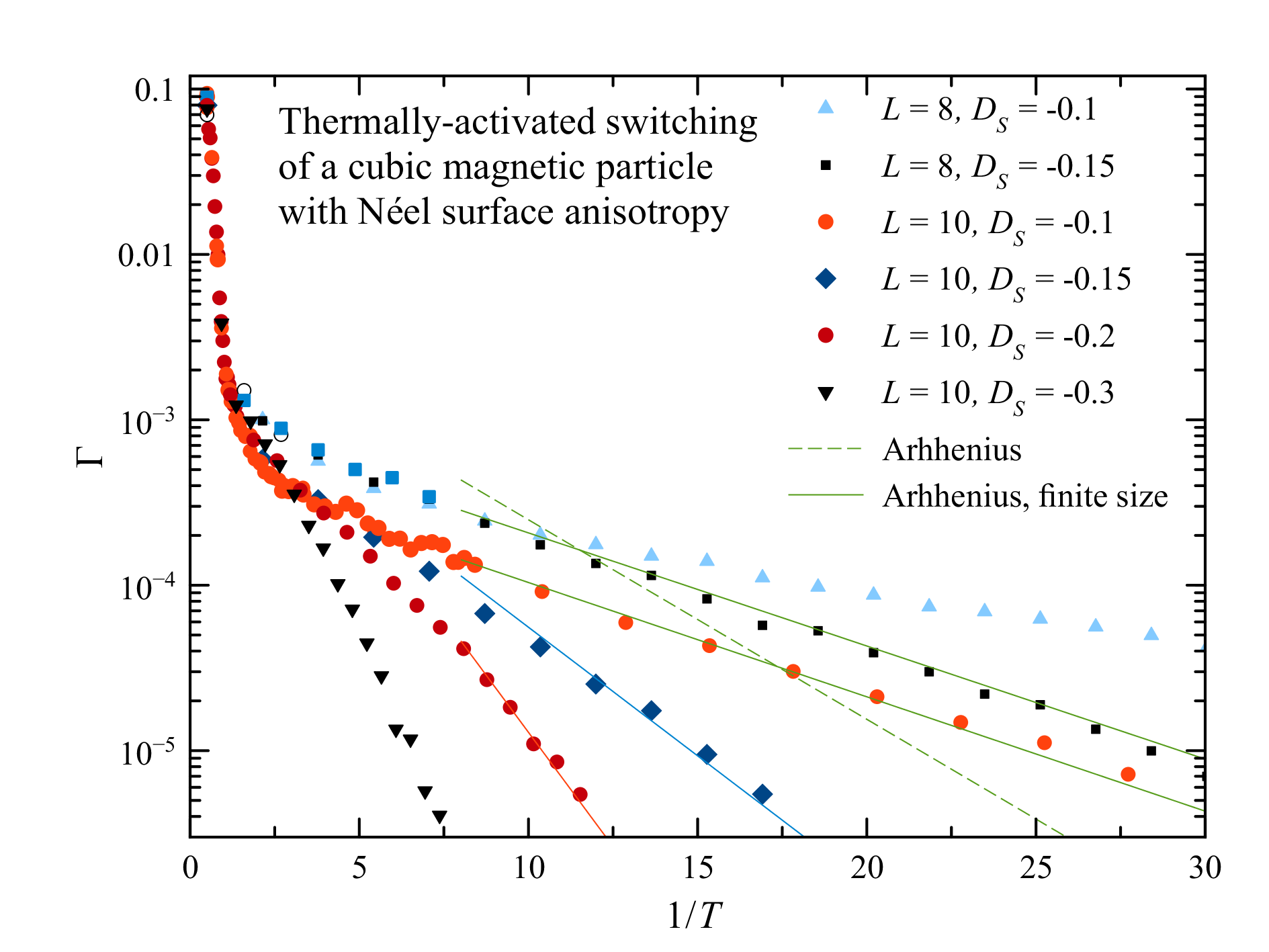
Figure 8: Thermally-activated switching of a magnetic particle with SA, considered as a many-spin system. Upper panel: An example of the time dependence of the particle’s magnetization components for a $4\times 4\times 4$ cube with $D_{S}=-0.1$ at $T=0.002$. Lower panel: Switching rate $\Gamma$ vs. the temperature for different particle’s sizes and $D_{S}$ values. All computations were done with the Landau-Lifshitz damping constant $\lambda=0.1$.

At low temperatures, the particle spends much time in the vicinity of the energy minima, making seldom switching to other energy minima over energy barriers. The characteristic time of the magnetization switching is important, for instance, for memory storage applications. The theory gives the Arrhenuis thermal activation law for the escape rate,

$$\Gamma=\Gamma_{0}e^{-U/T},$$ (60)

where $U$ is the energy barrier. In the case of a cubic particle with the surface anisotropy only in zero field, the barrier between the energy minima at $\left(1,1,1\right)$ and $\left(1,1,-1\right)$ is at $\left(1,1,0\right)$, and the value of the energy barrier following from Eq. (34) is given by

$$U=\frac{\mathcal{N}D_{S}^{2}}{36J}.$$ (61)

Switching rates for the additive core-surface effective anisotropy of magnetic particles within the single-spin model were calculated analytically in Ref. Déjardin et al. (2008) and analytically and numerically in Ref. Coffey et al. (2009). The ac susceptibility of assemblies of magnetic particles taking into account the effective cubic surface anisotropy and dipolar interaction between the particles was studied in Ref. Vernay et al. (2014).

To test the predictions above for the simplest case of a particle with the SA only, considered as a many-particle system, computations using the recently proposed pulse-noise method Garanin (2017) of solving the stochastic Landau-Lifshitz equation for a system of classical spins have been performed on cubic particles of cubic shape. This method replaces a quasi-continuous random field by equidistant pulses rotating all spins by random angles around random axes. Between the pulses, the deterministic Landau-Lifshitz equation is solved with an efficient high-order differential-equation solver. The overall speed of this method is defined by the latter, so the method is fast and suitable for computing on many-spin systems. Although the values of $D_{S}$ in these computations are negative, it does not matter because the effect of $D_{S}$ is quadratic. Switching was detected when any of the three magnetization components changed its sign.

The results are shown in Fig. 8. In the upper panel, jumping of the magnetization of a $4\times 4\times 4$ cube between the eight energy minima at a very low temperature is shown via the three magnetization components. The behavior is typical for the strong Lanadau-Lifshitz damping $\lambda=0.1$ used in these computations. The escape rates were computed with the method explained in the appendix to Ref. Garanin (3988) for the particle’s sizes $8\times 8\times 8$ and $10\times 10\times 10$ and different values of $D_{S}$. The results shown in the lower panel of Fig. 8 are in a fair accord with the theory, although the the barriers given by Eq. (61) and shown by the dotted line for the $10\times 10\times 10$ particle with $D_{S}=-0.1$ are too high. In fact, because of finite-size effects the barrier given by Eq. (61) should be lower, as discussed in Sec. VI. Here, replacing $D_{S}\Rightarrow\tilde{D}_{S}=(1-1.3/L)^{2}D_{S}$ corrects the barriers, as shown by the solid Ahhhenius lines with fitted prefactors $\Gamma_{0}$, as even small temperature dependence of the barrier strongly affects the prefactor and makes comparison with the theory for the latter hardly possible. Even without these corrections, one can see that the theory works comparing the slopes of the temperature dependence for $L=10$, $D_{S}=-0.1$ and $L=8$, $D_{S}=-0.15$. As the product $L^{3}D_{S}^{2}$ is nearly the same in both cases, the barriers should be nearly the same, that is indeed so, as can be seen in the figure.

IX Discussion

The cubic magnetic particle turned to be an easier object than the spherical particle for analytically calculating the second-order effective surface anisotropy since the linearized Laplace and Helmholtz equations for the deviations from the collinearity can be solved directly without using Green’s functions. This is, probably, a matter of luck since the analytical solution found for the cube cannot be easily generalized for a parallelepiped. On the other hand, the solution for the parallelepiped should be close to that for the cube as the numerically computed effective particle’s energy is practically independent of the particle’s aspect ratio, see Fig. 4.

The analytical solution found here allows to study the effect of screening of the surface perturbations at the distances of the domain-wall width $\delta$ in the presence of the uniaxial core anisotropy in the whole range of $L/\delta$, where $L$ is the particle’s linear size. These results are useful near the energy minima, where screening increases their stability. On the other hand, closer to the energy barriers screening is replaced by the anti-screening that leads to the instability of the linearized solution found here. It was shown that for small and moderate $L/\delta$ the effect of screening is very small, so that the applicability range of the additive approximation for the terms in the effective anisotropy is rather broad.

Magnetic particle of a cubic shape can be an analytically solvable model for other types of crystal lattices. It would be worth to investigate whether the sign of the effective cubic anisotropy is opposite for the fcc lattice, as has been found numerically for the spherical particles Yanes et al. (2007).

Another possible extension is analytically solving the discrete problem on the lattice instead of the Laplace equation in the continuous approximation since for small particles the finite-size effects are quite pronounced.